Decentralized Dynamic Parameter Identification of Modern Power Systems Using Ambient Measurements

Abstract

With the integration of high-penetration power electronics, the dynamic characteristics of modern power systems are jointly dominated by synchronous generators (SGs) and virtual synchronous machines (VSMs). However, the accuracy of these system parameters cannot always be guaranteed in real-world scenarios. To tackle this issue, we propose a robust parameter identification and correction framework based on trajectory sensitivity analysis and Pareto smoothed importance sampling (PSIS). First, to identify the sources of dynamic anomalies, we employ trajectory sensitivity analysis to quantify the impact of parameter variations and screen out key parameters for targeted identification. Subsequently, to utilize the readily available ambient measurements, we incorporate successive variational mode decomposition (SVMD). This method adaptively extracts the dominant variation modes, thereby recovering high-quality data for the identification process. Finally, to circumvent the weight degradation problem inherent in traditional particle filters, we propose a cost-effective PSIS algorithm to obtain the robust posterior distribution of modern system parameters. Simulation results demonstrate the excellent performance of the proposed method. It can not only precisely estimate the key parameters of both SGs and VSMs but also realize the automatic correction of dynamic models under complex operating scenarios.

1. Introduction

The modern power system is experiencing a profound transition towards a modern network characterized by the coexistence of synchronous generators (SGs) and power electronic-interfaced virtual synchronous machines (VSMs) [1]. In this complex environment, accurate dynamic modeling is the cornerstone of power system simulation, stability assessment, and control strategy design [2]. However, the parameters of these dynamic components, ranging from the inertia of aging SGs to the tunable control gains of VSMs, are often subject to significant uncertainty and time-varying drift. Relying on nominal or inaccurate parameters can lead to erroneous stability margins and, in extreme cases, catastrophic failures. A notable example is the 1996 Western North America blackout [3]. Post-event analysis revealed that the significant discrepancy between the simulation models and the actual system response, primarily caused by inaccurate dynamic parameters of generators and excitation systems, hindered the operators’ ability to foresee and prevent the instability [4]. Therefore, bridging the significant model–plant mismatch through accurate and robust parameter identification has become a major priority in ensuring the resilience of low-inertia power grids [5].

Despite the critical importance of parameter identification, several technical bottlenecks hinder its practical application in modern power grids. First, the modern system comprises a heterogeneous set of parameters, including both the physical coefficients of SGs and the flexible control gains of VSMs. Without a quantitative screening mechanism, it is often difficult to pre-determine which parameters will dominate the dynamic trajectory. Directly identifying all parameters may lead to over-parameterization and convergence issues due to the weak identifiability of non-dominant parameters [6]. Second, conventional identification strategies predominantly rely on data recorded during large disturbances, such as short circuits, to ensure sufficient system excitation. However, such severe fault events are infrequent in daily operations, making these methods unsuitable for routine, continuous monitoring [7]. Finally, with the proliferation of distributed VSMs, the dimension of the system state space expands explosively. Traditional centralized identification frameworks suffer from the curse of dimensionality and excessive communication burdens, rendering them inefficient for large-scale modern networks [8]. Collectively, these computational and operational hurdles drive the critical need for a hierarchical solution strategy capable of both accurately isolating dominant parameters within the high-dimensional space and efficiently estimating their values using a low-complexity algorithm.

In the realm of parameter identification, system inertia is universally recognized as a critical indicator governing frequency stability and is typically selected as the primary target for estimation [9]. The Kalman filter (KF) [10,11] and its variants, such as the unscented Kalman filter, are favored for their rigorous probabilistic framework, which offers superior robustness against measurement noise and process uncertainties [12]. Heuristic optimization algorithms, such as particle swarm optimization (PSO), utilize global search mechanisms to effectively avoid local optima, providing high-precision estimation for non-convex problems [13]. Concurrently, with the growing deployment of phasor measurement units (PMUs), deterministic approaches based on conventional swing equations have been widely explored. Specifically, the system total inertia can be estimated using the measured rate of change of frequency (RoCoF) at different nodes following disturbances [14,15]. To further enhance the accuracy, a polynomial fit method was introduced to simultaneously estimate the disturbance size and RoCoF [16]. Moreover, to avoid the numerical differentiation of rotor speeds, an online algorithm based on the dynamic regressor and mixing procedure was developed to estimate the overall inertia constants of larger-scale power systems [17]. However, these conventional centralized methodologies face a critical bottleneck. They heavily rely on infrequent large disturbances for sufficient excitation. These limitations regarding data availability render them unsuitable for the routine monitoring of modern power systems [18].

Even in the absence of major events such as short circuits or line trippings, PMU measurement data for voltage and power exhibit continuous, small-amplitude random fluctuations driven by real-time load changes. These data, originating from stochastic load variations, are referred to as ambient measurements [18]. To overcome the limitations of relying on infrequent fault events, recent scholarship has pivoted towards strategies that utilize these ubiquitous ambient measurements [17]. These approaches exploit the inherent stochastic fluctuations of loads to continuously excite system dynamics, enabling routine monitoring. Tuttelberg et al. pioneered this domain by establishing a unified framework that couples the inertia response with primary control, demonstrating the viability of extracting inertia solely from ambient data [19]. Building on this, Guo et al. advanced a data-driven estimator capable of simultaneously identifying the inertia of SGs and the virtual inertia of grid-following inverters [20]. However, its practical deployment is hindered by the stringent requirement for full-state observability, which is beyond the capabilities of current PMU infrastructure. To address estimation challenges from a statistical perspective, Bizzarri et al. utilized the covariance matrix of ambient signals to infer inertia and damping coefficients [21]. However, this method relies on linearization assumptions that may degrade in accuracy under highly non-linear operating conditions. Consequently, artificial intelligence techniques have been explored to capture such complex non-linearities; for instance, Poudyal et al. employed convolutional neural networks (CNNs) to map the relationships between time-series measurements and system momentum [22]. Despite their innovations, such “black-box” models suffer from poor interpretability, limiting their adoption in safety-critical operations. In light of these limitations, it is imperative to develop a robust and efficient solver that maintains high estimation accuracy even in the presence of arbitrary measurement noise.

To bridge these research gaps, this paper proposes a robust parameter identification and correction framework for hybrid power systems. In brief, we establish an ambient measurement-based decentralized Bayesian inference model to achieve scalable and robust parameter tracking. To address the challenge of parameter coupling in heterogeneous networks, trajectory sensitivity analysis is employed to quantify the impact of parameter variations on system dynamics, effectively screening out key parameters of synchronous generators and virtual synchronous machines for targeted identification. Meanwhile, to mitigate the adverse effects of non-stationarity and noise inherent in ambient data, successive variational mode decomposition (SVMD) is incorporated to extract dominant variation modes and construct high-quality measurement inputs. Furthermore, to overcome the sampling efficiency issues in solving the high-dimensional Bayesian model, a Pareto smoothed importance sampling (PSIS) algorithm is developed, ensuring the accurate acquisition of the posterior distribution for precise parameter estimation.

The main contributions of this paper are threefold:

1.

Unlike traditional methods that blindly select identification targets, the proposed mechanism employs trajectory sensitivity indices to reveal the coupling relationships between dynamic anomalies and specific physical parameters. By measuring the impact of parameter variations on system outputs, it provides a novel physical criterion for distinguishing the dominant parameters of both SGs and VSMs, significantly reducing the identification complexity and preventing over-parameterization.

2.

By fusing SVMD-based signal enhancement with a decentralized architecture, this work addresses the reliance of existing decentralized schemes on large disturbances. It simultaneously overcomes the “curse of dimensionality” inherent in centralized approaches and the data scarcity of fault events, enabling scalable and routine monitoring for large-scale modern power grids.

3.

Distinct from conventional particle filters or computationally expensive MCMC methods, the proposed PSIS algorithm fundamentally resolves the weight degeneracy issue and stabilizes importance weights. This ensures the high-precision estimation of non-Gaussian posteriors with improved sample efficiency, supporting the automatic and robust correction of dynamic models under complex operating scenarios.

The remainder of this paper is organized as follows. Section 2 constructs the non-linear state space model of the hybrid power system and formulates the ambient load stochasticity using differential equations and the Bayesian inference-based parameter identification problem. Section 3 establishes the parameter screening mechanism based on trajectory sensitivity analysis to identify dominant generator parameters. Section 4 presents the decentralized playback framework and introduces the SVMD-based signal enhancement technique to mitigate error accumulation. Section 5 details the proposed robust Bayesian inference strategy utilizing the Pareto smoothed importance sampling algorithm. Section 6 summarizes the overall implementation procedure. Finally, Section 7 validates the effectiveness and robustness of the proposed framework through simulation studies on a modified IEEE 39-bus system, followed by the conclusions and the future work in Section 8.

2. Problem Modeling

This section establishes the mathematical and theoretical groundwork for the proposed inertia identification strategy. We first formulate the non-linear state space dynamics of the hybrid power system comprising synchronous and virtual synchronous generators. Subsequently, we mathematically characterize the ambient load stochasticity, which serves as a persistent excitation source. Finally, the parameter identification task is cast within a probabilistic Bayesian inference framework.

2.1. Hybrid Power System Dynamic Formulation

This study investigates the transient behavior of a hybrid power network incorporating both conventional SGs and VSMs. From a control theory perspective, the dynamics of this heterogeneous network can be formulated as a general non-linear state space model given by

$$\left\{\begin{array}{c}\dot{\mathit{x}}\left(t\right)=\mathit{f}(\mathit{x}\left(t\right),\mathit{u}\left(t\right),\mathsf{\theta })\hfill \\ \mathit{y}\left(t\right)=\mathit{h}\left(\mathit{x}\right(t),\mathit{u}(t),\mathsf{\theta })\hfill \end{array}\right.$$

(1)

where the vector $\mathit{x}\in {\mathbb{R}}^n$ represents the system state variables, such as rotor angles, angular speeds, and internal voltages. The vector $\mathit{u}\in {\mathbb{R}}^m$ denotes the input vector, including load disturbances, while $\mathit{y}\in {\mathbb{R}}^p$ represents the measurement vector, containing variables like active power and voltage magnitudes. The vector $\mathsf{\theta }\in {\mathbb{R}}^k$ encapsulates the system parameters targeted for identification.

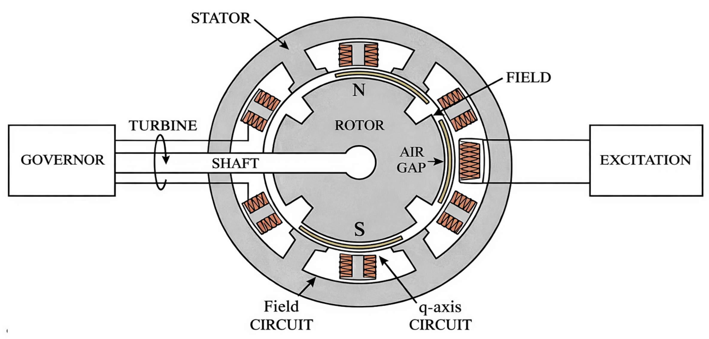
Specifically, the non-linear function $\mathit{f}$ is determined by the physical dynamics of the generation units. For the SGs, we employ a fourth-order two-axis model coupled with the IEEE-DC1A excitation system and the TGOV1 turbine governor framework, as illustrated in Figure 1. The differential equations governing the synchronous generator dynamics are expressed as [23]

$$\begin{array}{cc}\hfill T_{d0}^{\prime }{\displaystyle \frac{d{E}_q^{\prime }}{dt}}& =-E_q^{\prime }-(X_d-X_d^{\prime })I_d+E_{fd}\hfill \\ \hfill T_{q0}^{\prime }{\displaystyle \frac{d{E}_d^{\prime }}{dt}}& =-E_d^{\prime }+(X_q-X_q^{\prime })I_q\hfill \\ \hfill {\displaystyle \frac{d{\delta }_{SG}}{dt}}& ={\omega }_{SG}-{\omega }_g\hfill \\ \hfill {\displaystyle \frac{2H_g}{{\omega }_g}}{\displaystyle \frac{d{\omega }_{SG}}{dt}}& =T_M-P_e-D({\omega }_{SG}-{\omega }_g)\hfill \\ \hfill T_E{\displaystyle \frac{d{E}_{fd}}{dt}}& =-(K_E+S_E\left(E_{fd}\right))E_{fd}+V_R\hfill \\ \hfill T_F{\displaystyle \frac{d{R}_f}{dt}}& =-R_f+{\displaystyle \frac{K_F}{T_F}}{E}_{fd}\hfill \\ \hfill T_A{\displaystyle \frac{d{V}_R}{dt}}& =-V_R+K_A{R}_f-{\displaystyle \frac{K_A{K}_F}{T_F}}{E}_{fd}+K_A(V_{ref}-V)\hfill \\ \hfill T_{CH}{\displaystyle \frac{d{T}_M}{dt}}& =-T_M+P_{SV}\hfill \\ \hfill T_{SV}{\displaystyle \frac{d{P}_{SV}}{dt}}& =-P_{SV}+P_C-{\displaystyle \frac{1}{R_D}}\left({\displaystyle \frac{{\omega }_{SG}}{{\omega }_g}}-1\right)\hfill \end{array}$$

(2)

In the formulation above, $H_g$ denotes the inertia time constant. The parameters $T_{d0}^{\prime }$ through $T_{SV}$ denote the time constants for the stator transient response, excitation mechanism, and governor system. The symbols $X_d$ through $X_q^{\prime }$ represent the system reactance characteristics, while $K_A$, $K_E$, and $K_F$ are the gains associated with the exciter. The state variables include the transient voltages $E_q^{\prime }$ and $E_d^{\prime }$, the excitation states $E_{fd}$, $R_f$, and $V_R$, and the mechanical states comprising ${\delta }_{SG}$, ${\omega }_{SG}$, $T_M$, and $P_{SV}$.

Figure 1. Schematic diagram of the fourth-order two-axis synchronous generator model incorporating the IEEE-DC1A excitation system and the TGOV1 turbine governor.

Figure 1. Schematic diagram of the fourth-order two-axis synchronous generator model incorporating the IEEE-DC1A excitation system and the TGOV1 turbine governor.

For the inverter-based resources, the grid-forming virtual synchronous machine model is integrated into the analysis. Adopting the control structure outlined by Shen et al., the dynamic evolution is governed by [24]

$$\begin{array}{cc}\hfill {\displaystyle \frac{d{\delta }_{VSG}}{dt}}& ={\omega }_{VSG}-{\omega }_g\hfill \\ \hfill J{\displaystyle \frac{d{\omega }_{VSG}}{dt}}& =T_0-T_{em}-D_e({\omega }_{VSG}-{\omega }_g)\hfill \\ \hfill K{\displaystyle \frac{d{E}_{VSG}}{dt}}& =Q_0-Q_{em}-D_q(E_{VSG}-E_0)\hfill \end{array}$$

(3)

Here, the derived virtual inertia time constant is defined as $H_m=J{\omega }_g^2/\left(2S_{base}\right)$. The control coefficients include the equivalent damping $D_e$, the Q-V droop gain $D_q$, and the voltage integral gain K. The comprehensive parameter vector $\mathsf{\theta }$ encompasses all the aforementioned coefficients from both generator models.

Complementing the GFM units, the grid-following (GFL) converters are also modeled to capture their virtual inertia contributions. Unlike GFMs that mimic voltage sources, GFLs are typically controlled as current sources that track the grid phase via a phase-locked loop (PLL). To account for the virtual inertia characteristics, we adopt the control framework comprising an active power loop and a PLL dynamic model. The differential equations describing the GFL dynamics are

$$\begin{array}{cc}\hfill {\displaystyle \frac{d{x}_v}{dt}}& ={\displaystyle \frac{1}{T_v}}({\omega }_{PLL}-x_v)\hfill \\ \hfill {\displaystyle \frac{d{P}_v}{dt}}& ={\displaystyle \frac{1}{T_p}}\left(P_{vs}-K_v{\displaystyle \frac{d{x}_v}{dt}}-P_v\right)\hfill \\ \hfill {\displaystyle \frac{d{\theta }_{PLL}}{dt}}& ={\omega }_{PLL}+{\omega }_g\hfill \\ \hfill {\displaystyle \frac{d{x}_{PLL}}{dt}}& =Vsin(\theta -{\theta }_{PLL})\hfill \end{array}$$

(4)

where the auxiliary frequency variable is given by ${\omega }_{PLL}=K_{p}Vsin(\theta -{\theta }_{PLL})+K_i{x}_{PLL}$. In this model, $P_v$ and $P_{vs}$ represent the actual and reference active power outputs, while $x_v$ is an intermediate state variable for the inertia emulation loop. The parameter $K_v$ is directly related to the provided virtual inertia constant $H_v$ via $K_v=2H_v$. The time constants $T_v$ and $T_p$ characterize the virtual inertia control loop and the power converter response, respectively. The PLL dynamics are governed by the angle ${\theta }_{PLL}$, the internal state $x_{PLL}$, and the proportional–integral gains $K_p$ and $K_i$. The comprehensive parameter vector $\mathsf{\theta }$ encapsulates all the aforementioned coefficients from the synchronous, GFM, and GFL generator models.

2.2. Stochastic Modeling of Load Dynamics

To rigorously capture the ambient excitation utilized for identification, we model the load fluctuations using stochastic differential equations. The base load variations are modeled as a mean-reverting Ornstein–Uhlenbeck process [25]. Let $\chi \left(t\right)$ denote the stochastic component of the load, whose dynamics are governed by

$$d\chi \left(t\right)=\kappa \left(\overline{\chi }-\chi \left(t\right)\right)dt+{\sigma }_{L}d\mathcal{W}\left(t\right)$$

(5)

where $\overline{\chi }$ is the long-term mean, $\kappa$ represents the positive mean reversion speed, and ${\sigma }_L$ is the volatility parameter. The term $\mathcal{W}\left(t\right)$ denotes a standard Wiener process with independent Gaussian increments. The autocorrelation function of this process decays exponentially, which effectively mimics the temporal coherence of aggregate load changes.

To account for discrete switching events and sudden load steps, we augment the continuous model with a jump component. The composite dynamics are described by a jump diffusion SDE given by

$$d{\chi }_{total}\left(t\right)=\kappa (\overline{\chi }-\chi \left(t\right))dt+{\sigma }_{L}d\mathcal{W}\left(t\right)+\gamma d\mathcal{P}\left(t\right)$$

(6)

Here, $\mathcal{P}\left(t\right)$ is a Poisson process with intensity $\lambda$ representing the arrival rate of load jumps, and $\gamma$ denotes the random jump magnitude. This formulation ensures that the subsequent identification model is robust against non-Gaussian impulsive perturbations often observed in modern power grids.

2.3. Bayesian Identification Problem Formulation

Formally, the identification problem aims to infer the unknown system parameter vector $\mathsf{\theta }$ given the set of noisy measurements $\mathcal{D}$. The stochastic relationship between the parameters and the observed system response is governed by the non-linear observation equation

$$\mathit{y}=\mathit{h}\left(\mathsf{\theta }\right)+\mathit{e}$$

(7)

where $\mathit{e}$ denotes the measurement noise vector. Within the Bayesian framework, the system parameters are treated as random variables characterized by a posterior probability density function ${\pi }_{post}\left(\mathsf{\theta }\right|\mathcal{D})$. According to Bayes’ theorem [26], this posterior is proportional to the product of the likelihood function ${\pi }_{like}\left(\mathcal{D}\right|\mathsf{\theta })$ and the prior distribution ${\pi }_{prior}\left(\mathsf{\theta }\right)$ as expressed by

$${\pi }_{post}\left(\mathsf{\theta }\right|\mathcal{D})\propto {\pi }_{like}\left(\mathcal{D}\right|\mathsf{\theta }){\pi }_{prior}\left(\mathsf{\theta }\right)$$

(8)

To obtain a deterministic estimate for practical applications, we formulate the identification task as an optimization problem that seeks the parameter set maximizing the posterior probability. This maximum a posteriori estimator ${\widehat{\mathsf{\theta }}}_{MAP}$ is mathematically defined as

$${\widehat{\mathsf{\theta }}}_{MAP}=\arg \underset{\mathsf{\theta }}{\max }\left\{ln{\pi }_{like}\left(\mathcal{D}\right|\mathsf{\theta })+ln{\pi }_{prior}\left(\mathsf{\theta }\right)\right\}$$

(9)

where the logarithmic transformation is utilized to transform the product into a summation, thereby enhancing the numerical stability. The objective function defined above consists of a data fidelity term derived from the likelihood function and a regularization term derived from the prior distribution.

However, solving this optimization problem for the full-scale hybrid power system is hindered by substantial computational challenges arising from the high-dimensional parameter space and the complexity of global network simulations.

3. Key Parameter Selection via Trajectory Sensitivity Analysis

As discussed in Section 2.3, the high dimensionality of the parameter space poses a serious challenge for accurate identification. To address this, we employ sensitivity analysis as a systematic framework to screen out the dominant parameters. This section first formulates the general static sensitivity analysis to demonstrate its limitations in inertia identification and subsequently presents the trajectory sensitivity analysis as a necessary dynamic extension.

3.1. Sensitivity Analysis

Sensitivity analysis fundamentally quantifies how variations in system parameters propagate to the system outputs. In classical steady state analysis, the power system is governed by a set of algebraic power flow equations denoted by $\mathbf{0}=\mathit{g}({\mathit{x}}_{ss},\mathit{u},\mathsf{\theta })$, where ${\mathit{x}}_{ss}$ represents the steady state vector. The corresponding static measurement is given by ${\mathit{y}}_{ss}=\mathit{h}({\mathit{x}}_{ss},\mathsf{\theta })$. Mathematically, the general static sensitivity matrix ${\mathit{S}}_{static}$ is derived by the total differentiation of the algebraic constraints, which yields

$${\mathit{S}}_{static}={\displaystyle \frac{d{\mathit{y}}_{ss}}{d\mathsf{\theta }}}={\displaystyle \frac{\partial \mathit{h}}{\partial \mathsf{\theta }}}-{\displaystyle \frac{\partial \mathit{h}}{\partial {\mathit{x}}_{ss}}}{\left({\displaystyle \frac{\partial \mathit{g}}{\partial {\mathit{x}}_{ss}}}\right)}^{-1}{\displaystyle \frac{\partial \mathit{g}}{\partial \mathsf{\theta }}}$$

(10)

This analytical expression effectively measures the shift in the equilibrium point caused by parameter perturbations.

However, this static formulation is fundamentally ill-suited for identifying inertia parameters. For example, the inertia constant H governs the rate of change of the rotor speed and only manifests in the differential terms $\dot{\mathit{x}}$ of the system dynamics. In the steady state equilibrium where $\dot{\mathit{x}}=\mathbf{0}$, the terms associated with inertia vanish from the algebraic equations $\mathit{g}(·)$. Consequently, the static sensitivity of the system state with respect to inertia is theoretically zero. This physical characteristic necessitates the extension of sensitivity analysis from the static equilibrium domain to the time-domain trajectory to capture the transient behaviors where inertia plays a dominant role.

3.2. Trajectory Sensitivity Analysis

To rigorously quantify the parameter influence throughout the dynamic process, we adopt trajectory sensitivity analysis [27]. This method generalizes the sensitivity concept to dynamic systems by defining sensitivity as a time-varying function. Let the i-th output variable $y_i\left(t\right)$ from the measurement vector be a function of the parameter ${\theta }_j$. The trajectory sensitivity is defined as the time-varying partial derivative ${\lambda }_{ij}\left(t\right)=\partial y_i\left(t\right)/\partial {\theta }_j$.

3.2.1. Trajectory Sensitivity Formulation

By differentiating the general non-linear dynamic equations (1) with respect to the parameter ${\theta }_j$, the time evolution of the sensitivity vector ${\mathsf{\lambda }}_j\left(t\right)$ is obtained. It is governed by the following linear time-varying differential equation:

$${\dot{\mathsf{\lambda }}}_j={\displaystyle \frac{\partial \mathit{f}}{\partial \mathit{x}}}{\mathsf{\lambda }}_j+{\displaystyle \frac{\partial \mathit{f}}{\partial {\theta }_j}},{\mathsf{\lambda }}_j\left(t_0\right)=\mathbf{0}$$

(11)

where the term $\partial \mathit{f}/\partial \mathit{x}$ is the Jacobian matrix, which characterizes the system stability characteristics along the trajectory. The term $\partial \mathit{f}/\partial {\theta }_j$ represents the direct forcing function, indicating the immediate impact of the parameter on the state derivatives. By solving this equation simultaneously with the original system dynamics, we obtain the sensitivity trajectory, which precisely describes how the system dynamic response deviates over time due to parameter perturbations.

3.2.2. Relative Sensitivity Index

Since the parameters in $\mathsf{\theta }$ possess different physical units and magnitudes, a direct comparison of the absolute sensitivities ${\lambda }_{ij}$ would be biased. To allow for a fair ranking, we introduce the dimensionless relative trajectory sensitivity ${\overline{S}}_{ij}\left(t\right)$, defined as

$${\overline{S}}_{ij}\left(t\right)={\displaystyle \frac{{\theta }_{j,0}}{y_{i,0}}}·{\lambda }_{ij}\left(t\right)={\displaystyle \frac{{\theta }_{j,0}}{y_{i,0}}}·{\displaystyle \frac{\partial y_i\left(t\right)}{\partial {\theta }_j}}$$

(12)

where ${\theta }_{j,0}$ and $y_{i,0}$ are the nominal values of the parameter and the output variables used for normalization.

To quantify the global influence of a parameter ${\theta }_j$ over the entire observation window from time 0 to T, we construct the Euclidean sensitivity index, denoted as ${\mathcal{I}}_j$, which is calculated as

$${\mathcal{I}}_j=\sqrt{{\displaystyle \frac{1}{T}}{\int }_0^T{\left({\overline{S}}_{ij}\left(t\right)\right)}^{2}dt}$$

(13)

3.2.3. Parameter Screening Strategy

The magnitude of ${\mathcal{I}}_j$ serves as a direct indicator of parameter identifiability. A larger ${\mathcal{I}}_j$ implies that variations in parameter ${\theta }_j$ cause significant deviations in the output trajectory, making such parameters easier to estimate from measurements. Conversely, parameters with ${\mathcal{I}}_j\approx 0$ indicate that the system response is insensitive to their variations and thus these parameters contribute minimally to the output dynamics.

Based on the calculated indices, we propose a systematic screening strategy to partition the high-dimensional parameter space. We define a sensitivity threshold $\tau$ to classify the parameters. Specifically, parameters satisfying ${\mathcal{I}}_j>\tau$ are identified as dominant parameters and are grouped into the subset ${\mathsf{\theta }}_{est}$ for subsequent estimation. The remaining parameters are categorized as nuisance parameters and are fixed to their nominal values. This procedure effectively reduces the dimensionality of the inference problem while ensuring that the critical dynamic characteristics are preserved for accurate identification.

4. Ambient Measurement-Based Decentralized Framework

This section articulates an ambient measurement-based decentralized framework that decouples the local generator dynamics from the external grid.

4.1. Decentralized Playback Mechanism

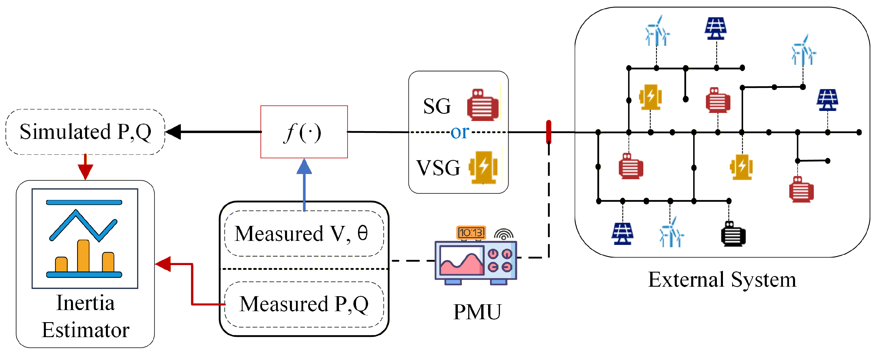
The fundamental principle of the decentralized approach is to isolate the target generator from the complex external power system, thereby transforming the high-dimensional system-level estimation problem into a series of independent single-machine sub-problems. For a specific generator located at bus i, the phasor measurement unit (PMU) provides high-resolution time-series data of the voltage magnitude $V_i\left(t\right)$ and phase angle ${\theta }_i\left(t\right)$.

In the proposed framework, as depicted in Figure 2, motivated by the event playback scheme, these ambient measurements are treated as deterministic inputs that drive the local generator dynamics. Let ${\mathit{x}}_i$ denote the state vector and ${\mathsf{\theta }}_i\subset \mathsf{\theta }$ denote the local parameter set. By incorporating the measured input vector ${\mathit{u}}_i\left(t\right)={[V_i\left(t\right),{\theta }_i\left(t\right)]}^T$, the decoupled dynamic model for the i-th unit can be reformulated as

$${\dot{\mathit{x}}}_i\left(t\right)={\mathit{f}}_i\left({\mathit{x}}_i\left(t\right),{\mathit{u}}_i\left(t\right),{\mathsf{\theta }}_i\right)$$

(14)

This formulation effectively opens the feedback loop from the grid, treating the interconnection variables as known disturbances.

Figure 2. Schematic diagram of the proposed decentralized playback framework utilizing ambient PMU measurements.

Figure 2. Schematic diagram of the proposed decentralized playback framework utilizing ambient PMU measurements.

Specifically, the system inertia $H_i$ governs the electromechanical dynamics through the swing equation, where the electrical power $P_{e,i}$ acts as the coupling term. Unlike fault-based schemes that span only a few seconds, the ambient measurement-based approach collects data over a significantly longer time window. By substituting the measured trajectories into the stator algebraic equations, the output active power $P_{sim,i}\left(t\right)$ and reactive power $Q_{sim,i}\left(t\right)$ are reconstructed via the $d-q$ axis projection

$$\begin{array}{cc}\hfill v_{d,i}\left(t\right)& =V_i\left(t\right)sin({\delta }_i\left(t\right)-{\theta }_i\left(t\right))\hfill \\ \hfill v_{q,i}\left(t\right)& =V_i\left(t\right)cos({\delta }_i\left(t\right)-{\theta }_i\left(t\right))\hfill \\ \hfill P_{sim,i}\left(t\right)& =v_{d,i}\left(t\right)I_{d,i}({\mathit{x}}_i,{\mathit{u}}_i)+v_{q,i}\left(t\right)I_{q,i}({\mathit{x}}_i,{\mathit{u}}_i)\hfill \\ \hfill Q_{sim,i}\left(t\right)& =v_{q,i}\left(t\right)I_{d,i}({\mathit{x}}_i,{\mathit{u}}_i)-v_{d,i}\left(t\right)I_{q,i}({\mathit{x}}_i,{\mathit{u}}_i)\hfill \end{array}$$

(15)

where $v_{d,i},v_{q,i}$ are the terminal voltages projected onto the rotor reference frame, and $I_{d,i},I_{q,i}$ are the stator currents derived from the transient model in (2). These simulated outputs act as the play-out functions and are compared with the measured power to construct the likelihood function, ensuring that the identification process is immune to topology errors in the external network.

4.2. The Challenge of Error Accumulation

While the decentralized scheme offers computational advantages, its application to ambient measurements introduces a unique error accumulation phenomenon. In fault-based methods, the high signal-to-noise ratio during large disturbances masks measurement errors. However, ambient measurements rely on small signal variations accumulated over an extended duration, making them highly susceptible to PMU measurement noise.

Let the measured voltage magnitude and angle be expressed as $V_m\left(t\right)=V\left(t\right)+e_v\left(t\right)$ and ${\theta }_m\left(t\right)=\theta \left(t\right)+e_{\theta }\left(t\right)$, where $e_v$ and $e_{\theta }$ denote the PMU measurement noise. In recent years, the majority of experimental studies have modeled these measurement errors using Gaussian distributions [28]. However, recent studies have demonstrated that the noise follows a non-Gaussian distribution, such as the Beta distribution, which better reflects complex real-world anomalies [29]. When these noisy inputs are fed into the decentralized model, they propagate into the output active and reactive power calculations. According to the generator stator equations, the output powers are explicitly coupled with these stochastic inputs:

$$P_{sim}\left(t\right)={\displaystyle \frac{E^{\prime }\left(t\right)(V\left(t\right)+e_v)}{X_d^{\prime }}}sin(\delta \left(t\right)-(\theta \left(t\right)+e_{\theta }))$$

(16)

$$Q_{sim}\left(t\right)=-{\displaystyle \frac{{(V\left(t\right)+e_v)}^2}{X_d^{\prime }}}+{\displaystyle \frac{E^{\prime }\left(t\right)(V\left(t\right)+e_v)}{X_d^{\prime }}}cos(\delta \left(t\right)-(\theta \left(t\right)+e_{\theta }))$$

(17)

where $E^{\prime }$, $\delta$, and $X_d^{\prime }$ represent the internal voltage, rotor angle, and transient reactance, respectively. As the time window extends, the cumulative effect of the noise terms $e_v$ and $e_{\theta }$ does not average out due to the non-linear coupling. This results in significant divergence between the simulated and true power trajectories, rendering the decentralized Bayesian inference inaccurate without effective noise mitigation.

4.3. Signal Enhancement via Successive Variational Mode Decomposition

To mitigate the error accumulation identified above, it is imperative to filter the input measurements. Traditional filters often struggle to separate the stochastic system dynamics from measurement noise due to spectral overlap. Therefore, we employ SVMD. Unlike standard variational mode decomposition (VMD), SVMD iteratively extracts the intrinsic mode functions, making it computationally efficient for processing long-duration ambient data.

The mathematical objective of SVMD is to decompose the noisy input signal into a sequence of discrete modes $u_k\left(t\right)$. Distinct from standard VMD, which requires a pre-defined mode number K, the total number of extracted modes in SVMD is adaptively determined by a convergence tolerance parameter $\gamma$. Specifically, the iterative extraction continues until the ratio of the residual signal energy to the original signal energy falls below $\gamma$. This mechanism ensures that all significant dynamic components are captured without over-decomposition. For the k-th mode, the algorithm seeks to minimize its bandwidth around a center frequency ${\omega }_k$. The constrained optimization problem for the k-th mode is formulated as

$$\underset{u_k,{\omega }_k}{min}{\mathcal{J}}_k=\alpha {∥{\partial }_t\left[\left({\delta }_D\left(t\right)+{\displaystyle \frac{j}{\pi t}}\right)\ast u_k\left(t\right)\right]e^{-j{\omega }_{k}t}∥}_2^2+{∥f\left(t\right)-\sum _{i=1}^{k-1}{u}_i\left(t\right)-u_k\left(t\right)∥}_2^2$$

(18)

where ${\delta }_D$ represents the Dirac distribution and ∗ denotes convolution. The penalty parameter $\alpha$ balances the bandwidth constraint and reconstruction fidelity.

To efficiently solve this constrained optimization problem, we adopt the Alternate Direction Method of Multipliers (ADMM). This approach transforms the original problem into an unconstrained formulation by constructing an augmented Lagrangian function, incorporating a Lagrange multiplier $\lambda \left(t\right)$ to enforce the reconstruction constraint. The solution is obtained by finding the saddle point of the augmented Lagrangian, which involves alternately updating the mode $u_k$, the center frequency ${\omega }_k$, and the multiplier $\lambda$ in the spectral domain.

Solving the problem yields the iterative update rules in the frequency domain:

$${\widehat{u}}_k^{n+1}\left(\omega \right)={\displaystyle \frac{\widehat{f}\left(\omega \right)-{\sum }_{i=1}^{k-1}{\widehat{u}}_i\left(\omega \right)}{1+2\alpha {(\omega -{\omega }_k^n)}^2}}$$

(19)

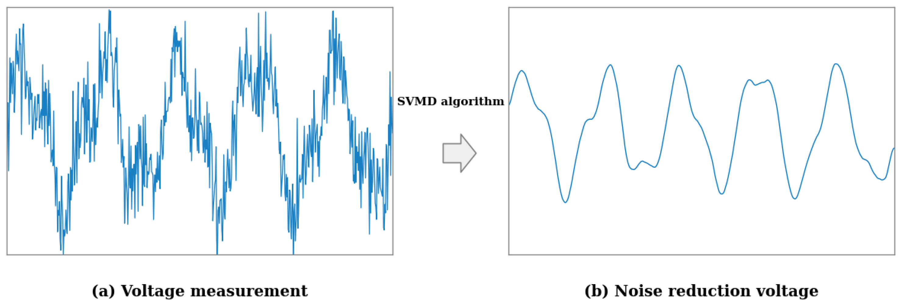
Upon decomposing the signal, a selection strategy is employed to distinguish between physical variations and noise. Modes characterizing high-frequency noise components are identified and discarded. The denoised voltage signals are then reconstructed solely from the selected modes, as visually demonstrated in Figure 3. By utilizing these cleaned voltage trajectories to drive the decentralized model, the error accumulation described in (2) and (3) is significantly suppressed, ensuring the fidelity of the Bayesian inference.

5. Robust Bayesian Inference via Pareto Smoothed Importance Sampling

This section introduces the importance sampling method first. Then, the Pareto smoothed importance sampling algorithm is proposed to address the numerical instability issues common in Bayesian computation methods.

5.1. Importance Sampling and Weight Degeneracy

Bayesian inference typically requires computing the expectation of a specific function $h\left(\mathsf{\theta }\right)$ under the target posterior distribution $\pi \left(\mathsf{\theta }\right|\mathcal{D})$. However, in complex power system models, the posterior is often analytically intractable and difficult to sample from directly due to the unknown normalizing constant. To address this, importance sampling (IS) introduces a tractable proposal distribution $q\left(\mathsf{\theta }\right)$ from which samples can be readily generated. The fundamental idea is to correct the distributional bias using importance weights, thereby approximating the integral via Monte Carlo averaging.

Let ${\left\{{\mathsf{\theta }}^{\left(s\right)}\right\}}_{s=1}^S$ be a set of S independent samples drawn from the proposal $q\left(\mathsf{\theta }\right)$. The importance weight for the s-th sample is defined as the ratio of the target density to the proposal density:

$$w^{\left(s\right)}={\displaystyle \frac{\pi \left({\mathsf{\theta }}^{\left(s\right)}\right|\mathcal{D})}{q\left({\mathsf{\theta }}^{\left(s\right)}\right)}}$$

(20)

Since the normalizing constant of the posterior is generally unknown, the self-normalized importance sampling (SNIS) estimator is typically employed. The expectation is approximated as

$${\mathbb{E}}_{\pi }\left[h\left(\mathsf{\theta }\right)\right]\approx {\displaystyle \frac{{\sum }_{s=1}^S{w}^{\left(s\right)}h\left({\mathsf{\theta }}^{\left(s\right)}\right)}{{\sum }_{s=1}^S{w}^{\left(s\right)}}}$$

(21)

This estimator is asymptotically unbiased and consistent, provided that the support of the proposal $q\left(\mathsf{\theta }\right)$ covers that of the target $\pi \left(\mathsf{\theta }\right|\mathcal{D})$.

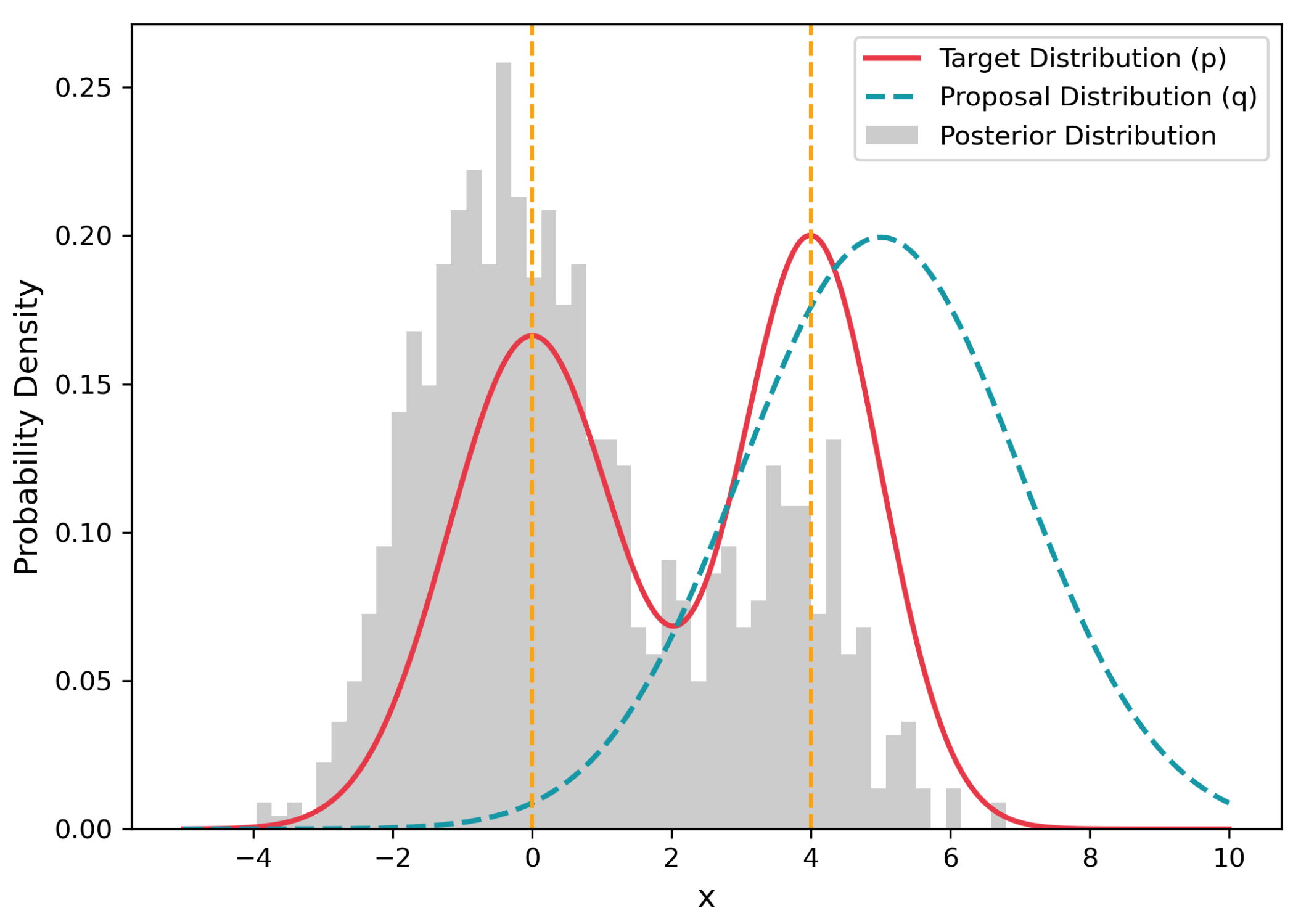
Despite its theoretical soundness, the practical performance of IS is heavily dependent on the quality of the proposal distribution. A critical challenge arises when there is a significant mismatch between the high-probability regions of the proposal and the target distributions. This phenomenon, known as weight degeneracy, is visually illustrated in Figure 4. As depicted, the proposal distribution $q\left(\mathsf{\theta }\right)$ (indicated by the dashed blue line) fails to adequately cover the significant mass of the target distribution $\pi \left(\mathsf{\theta }\right|\mathcal{D})$ (solid red line), specifically missing the left mode. Consequently, samples drawn from these tail regions—where the target density is high but the proposal density is low—yield extremely large importance weights. These rare but highly weighted samples dominate the summation in (8), leading to severe estimation instability.

5.2. Pareto Smoothed Importance Sampling

To rigorously mitigate the infinite variance problem associated with the heavy-tailed weight distribution, we employ PSIS [30]. This method relies on the theoretical foundation of Extreme Value Theory, specifically the Pickands–Balkema–de Haan theorem, which states that the distribution of excesses over a sufficiently high threshold asymptotically converges to a generalized Pareto distribution (GPD).

The PSIS procedure begins by sorting the raw importance weights in ascending order, denoted by $w^{\left(1\right)}\le \cdots \le w^{\left(S\right)}$. A cutoff index is established to isolate the M largest weights, which constitute the distribution tail. We fit a GPD to these M tail samples to obtain the estimated shape parameter $\widehat{k}$ and scale parameter $\widehat{\sigma }$. The probability density function of the GPD is given by

$$f(y;k,\sigma )={\displaystyle \frac{1}{\sigma }}{\left(1+{\displaystyle \frac{ky}{\sigma }}\right)}^{-(1+1/k)},y\ge 0$$

(22)

The core innovation of PSIS lies in its smoothing mechanism. To suppress the variance caused by sporadic outliers, the raw weights in the tail are replaced by the expected order statistics of the fitted GPD. Specifically, for the tail indices $s>S-M$, the smoothed weights ${\tilde{w}}^{\left(s\right)}$ are computed as

$${\tilde{w}}^{\left(s\right)}=F^{-1}\left({\displaystyle \frac{s-(S-M)-0.5}{M}};\widehat{k},\widehat{\sigma }\right)$$

(23)

where $F^{-1}$ represents the inverse cumulative distribution function of the GPD. The remaining non-tail weights are preserved. This transformation effectively regularizes the extreme weights, trading a negligible amount of bias for a significant reduction in estimator variance.

Furthermore, the estimated shape parameter $\widehat{k}$ serves as a critical diagnostic metric for evaluating the reliability of the approximation. The interpretation of $\widehat{k}$ is as follows:

• If $\widehat{k}<0.5$, the distribution of importance ratios has finite variance, ensuring that the Central Limit Theorem holds and convergence is fast.
• If $0.5\le \widehat{k}<0.7$, the variance is infinite, but the mean exists. The Generalized Central Limit Theorem applies, and the PSIS estimate remains reliable, albeit with slower convergence.
• If $\widehat{k}>0.7$, the tail is too heavy, indicating a severe mismatch between the proposal and target distributions, rendering the estimate unstable.

In our framework, $\widehat{k}$ acts as a real-time indicator, validating whether the decentralized proposal sufficiently covers the posterior.

6. Implementation Framework

The proposed robust parameter identification methodology integrates the theoretical modules discussed in the preceding sections into a coherent, closed-loop pipeline. The framework is designed to address the specific challenges of modern power systems: high dimensionality, data quality degradation in ambient conditions, and computational instability in probabilistic inference.

The execution flow, as outlined in Algorithm 1, proceeds in three sequential stages. Initially, the trajectory sensitivity analysis (TSA) acts as a physical filter. By computing the Euclidean sensitivity index ${\mathcal{I}}_j$, it effectively partitions the parameter space, locking nuisance parameters and isolating the dominant subset ${\mathsf{\theta }}_{est}$ for estimation. This step significantly lowers the computational barrier for subsequent inference.

Algorithm 1 Robust Decentralized Parameter Identification Framework

Require:  Raw Ambient Measurements: $V_{meas}\left(t\right),{\theta }_{meas}\left(t\right),P_{meas}\left(t\right)$ Ensure:  Estimated Parameter ${\widehat{\mathsf{\theta }}}_{MAP}$, Posterior Distribution ${\pi }_{post}\left(\mathsf{\theta }\right)$   1: // Stage 1: Pre-Processing and Screening   2: Initialize nominal system parameters.   3: Compute sensitivity index ${\mathcal{I}}_j$ for all parameters via TSA.   4: Select dominant parameters ${\mathsf{\theta }}_{est}=\{{\theta }_j\mid {\mathcal{I}}_j>\tau \}$.   5: Fix remaining parameters to nominal values.   6: // Stage 2: Signal Enhancement (SVMD)   7: Decompose noisy input $V_{meas}\left(t\right)$ into modes ${\left\{m_k\left(t\right)\right\}}_{k=1}^K$.   8: Identify dominant physical modes $k\in {\mathsf{\Omega }}_{phy}$.   9: Reconstruct clean input $V_{clean}\left(t\right)\leftarrow {\sum }_{k\in {\mathsf{\Omega }}_{phy}}{m}_k\left(t\right)$. 10: (Repeat SVMD process for angle ${\theta }_{meas}\left(t\right)$ to obtain ${\theta }_{clean}\left(t\right)$). 11: // Stage 3: Decentralized Bayesian Inference via PSIS 12: Initialize prior ${\pi }_{prior}\left({\mathsf{\theta }}_{est}\right)$ and proposal $q\left({\mathsf{\theta }}_{est}\right)$. 13: Draw S samples $\left\{{\mathsf{\theta }}^{\left(s\right)}\right\}$ from $q\left({\mathsf{\theta }}_{est}\right)$. 14: for $s=1$ to S do 15:      Decentralized Playback Simulation: 16:      Input $V_{clean}\left(t\right),{\theta }_{clean}\left(t\right)$ into local dynamic model (2) or (3). 17:      Compute simulated active power $P_{sim}^{\left(s\right)}\left(t\right)$. 18:      Calculate unnormalized weight $w^{\left(s\right)}$ based on likelihood between $P_{sim}^{\left(s\right)}$ and $P_{meas}$. 19: end for 20: // Stage 4: Posterior Smoothing and Estimation 21: Sort weights and fit GPD to the M tail samples. 22: Compute shape parameter $\widehat{k}$ for diagnostic check. 23: if  $\widehat{k}>0.7$  then 24:    Refine $q\left({\mathsf{\theta }}_{est}\right)$. 25: else 26:    Compute smoothed weights $\left\{{\tilde{w}}^{\left(s\right)}\right\}$ using GPD quantiles. 27:    Construct posterior approximation ${\widehat{\pi }}_{post}\left({\mathsf{\theta }}_{est}\right)$. 28:    Extract MAP estimate ${\widehat{\mathsf{\theta }}}_{MAP}\leftarrow \arg \max {\widehat{\pi }}_{post}\left({\mathsf{\theta }}_{est}\right)$. 29: end if 30: return  ${\widehat{\mathsf{\theta }}}_{MAP}$

Following the screening, the raw ambient data collected from PMUs undergo signal enhancement. The SVMD algorithm decomposes the voltage magnitude and angle measurements into intrinsic modes $m_k\left(t\right)$. By reconstructing the signal solely from low-frequency electromechanical modes, we effectively strip away high-frequency measurement noise that would otherwise accumulate in the decentralized playback model.

Finally, the core estimation is executed via the decentralized Bayesian inference engine. The cleaned measurements drive the local generator models to generate “played-back” power trajectories. The discrepancy between these simulated and measured outputs shapes the likelihood function. To explore the posterior distribution robustly, the PSIS algorithm is employed. It not only provides the maximum a posteriori (MAP) estimate ${\widehat{\mathsf{\theta }}}_{MAP}$ but also utilizes the shape parameter $\widehat{k}$ as a runtime diagnostic to ensure the statistical validity of the results.

7. Case Study

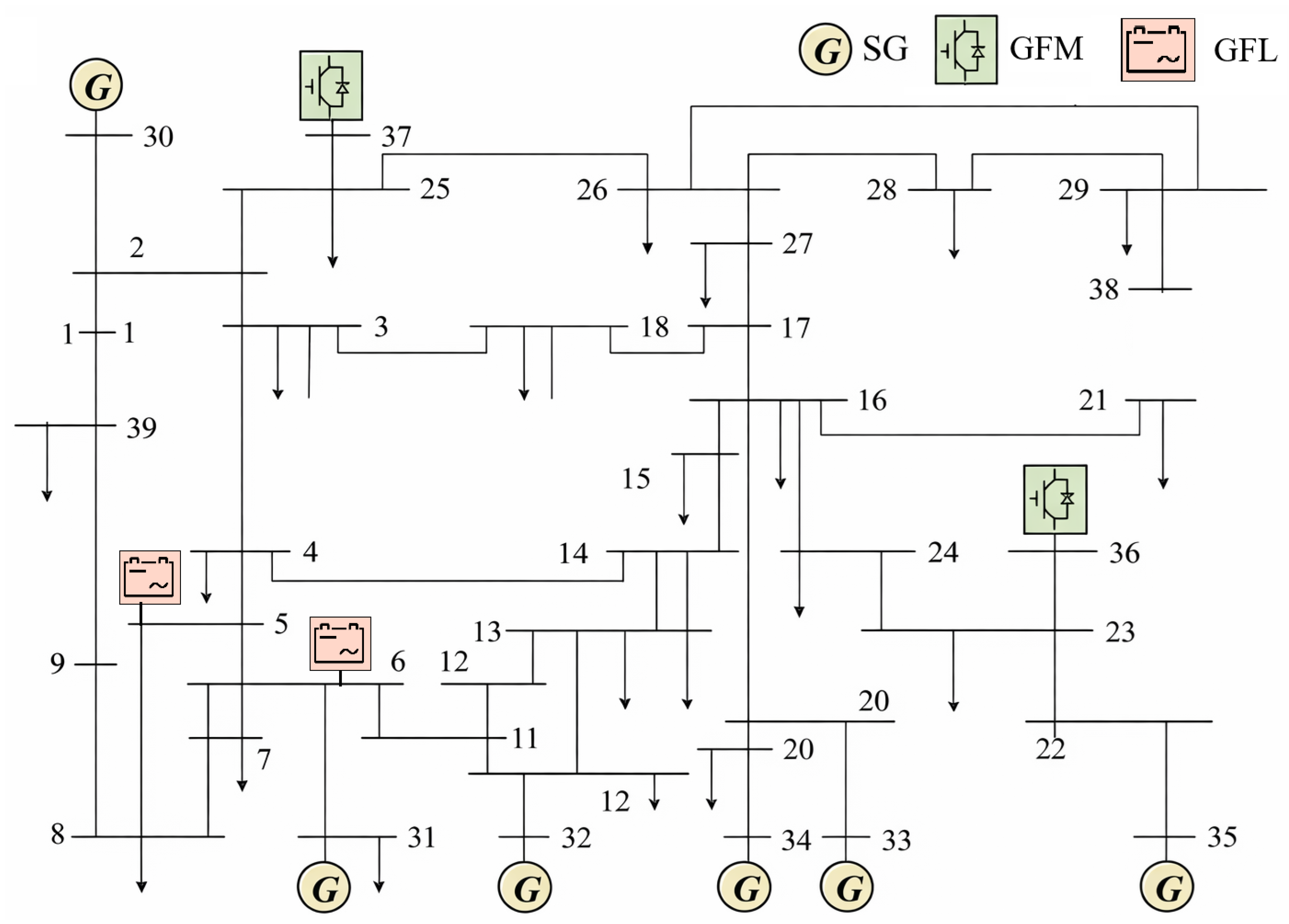
In this section, we validate the effectiveness of the proposed method using a modified IEEE 39-bus test system, as illustrated in Figure 5. To simulate a modern heterogeneous power network, the system is equipped with three distinct types of generation units: traditional SGs, grid-forming (GFM) virtual synchronous generators, and grid-following (GFL) converters. The spatial distribution of these 10 units is as follows: six SGs are connected to buses 30, 31, 32, 33, 34, and 35; two GFL converters are deployed at buses 5 and 6; and two GFM-VSGs are integrated into buses 36 and 37.

To generate the necessary dynamic trajectories for analysis, stochastic load perturbations are applied across the network, consistent with the ambient measurement conditions described in Section 2. To mimic realistic sensing environments and verify the method’s resilience to different noise statistics, the acquired PMU data are corrupted with controlled noise injections. In addition to standard Gaussian white noise, non-Gaussian Beta noise is incorporated into the subsequent experiments. This setup provides a robust benchmark to test the proposed framework’s ability to handle complex measurement anomalies.

7.1. Parameter Sensitivity Analysis on IEEE 39-Bus System

Before conducting parameter estimation, it is essential to evaluate the identifiability of the model parameters to avoid over-parameterization. We employ the TSA method to quantify the impacts of different generator parameters on the system’s dynamic response. Specifically, the sensitivity indices are computed using finite difference approximation. Each target parameter is individually perturbed by a small variation of $ϵ=0.001$ from its nominal value. The sensitivity magnitude is then quantified by calculating the Frobenius norm of the deviation matrix between the perturbed and baseline trajectories over the observation window, normalized by the perturbation size $ϵ$. Based on the sensitivity ranking, an adaptive screening strategy is applied. For each type of power source, the truncation threshold $\tau$ is defined as 50% of the maximum relative sensitivity observed within the specific category. Consequently, only parameters with sensitivity values exceeding this threshold are retained as dominant parameters for identification, while insensitive parameters are fixed at their nominal values. By calculating the relative sensitivity of the output trajectories with respect to variations in generator parameters, we can determine the dominant parameters that can be accurately estimated.

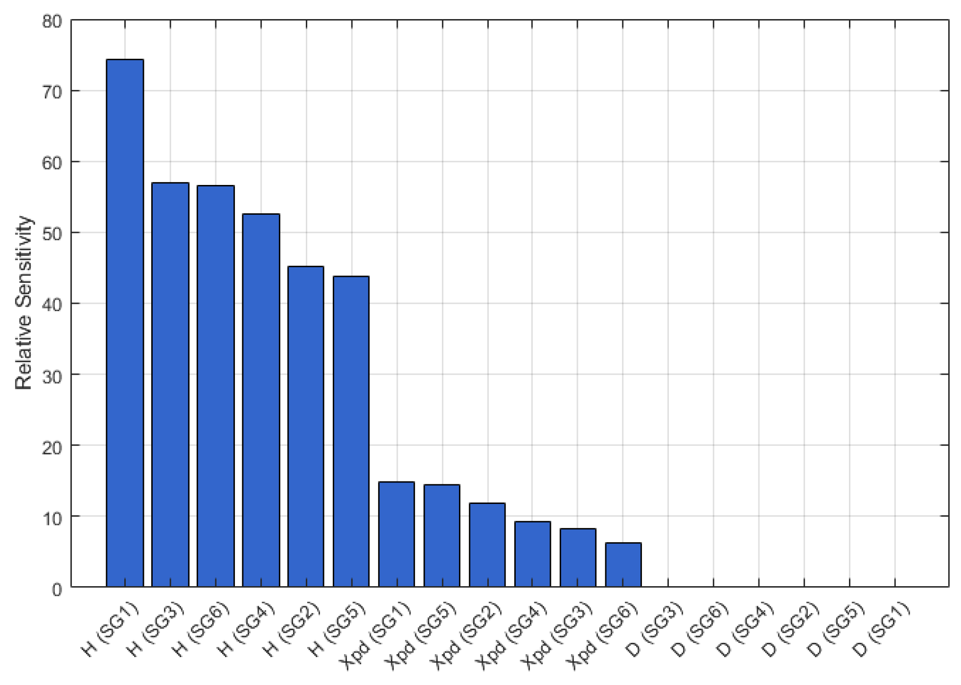
The results of the sensitivity analysis are presented in Figure 6, Figure 7 and Figure 8. Figure 6 illustrates the relative sensitivities of the parameters for SGs. It can be observed that the inertia time constant H exhibits the highest sensitivity compared to other parameters, such as the transient reactance $X_{pd}$ and damping coefficient D. This indicates that the dynamic response of the SG is predominantly determined by its inertia, making H the most identifiable parameter.

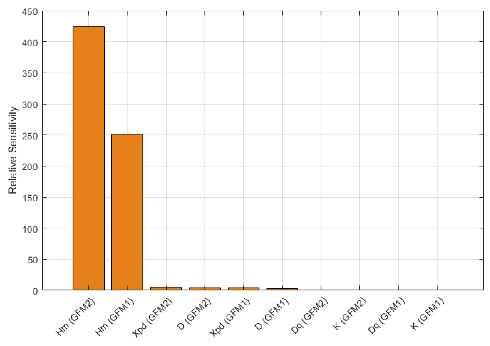
Similarly, for the grid-forming VSGs, as shown in Figure 7, the virtual inertia constant $H_m$ demonstrates significantly higher sensitivity than other control parameters, such as the reactive power droop $D_q$ or the voltage coefficient K. This confirms that the inertial response is the dominant characteristic of the GFM control loop under the tested conditions.

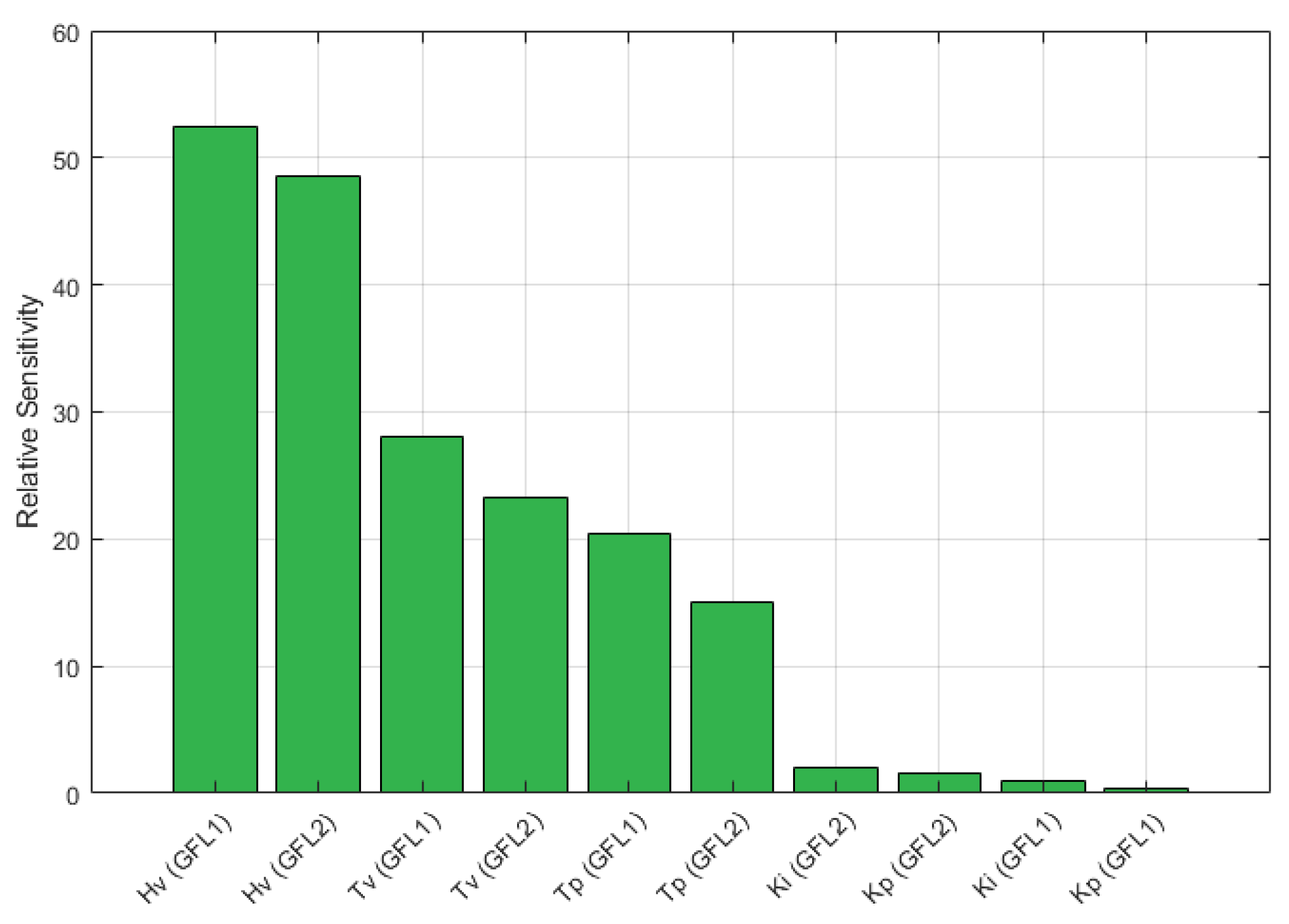
For the grid-following converters, the sensitivity analysis results are depicted in Figure 8. Consistent with the previous cases, the virtual inertia constant $H_v$ shows the highest relative sensitivity. However, it is worth noting that the time constants associated with the virtual inertia loop and active power loop, specifically $T_v$ and $T_p$, also exhibit considerable sensitivity. Nevertheless, $H_v$ remains the primary factor influencing the trajectory, justifying the focus of this paper on inertia estimation. The dominance of inertia parameters ($H,H_m,H_v$) across all three generator types validates the feasibility of the proposed Bayesian inference framework for accurate inertia tracking.

7.2. Validation of SVMD-Based Denoising

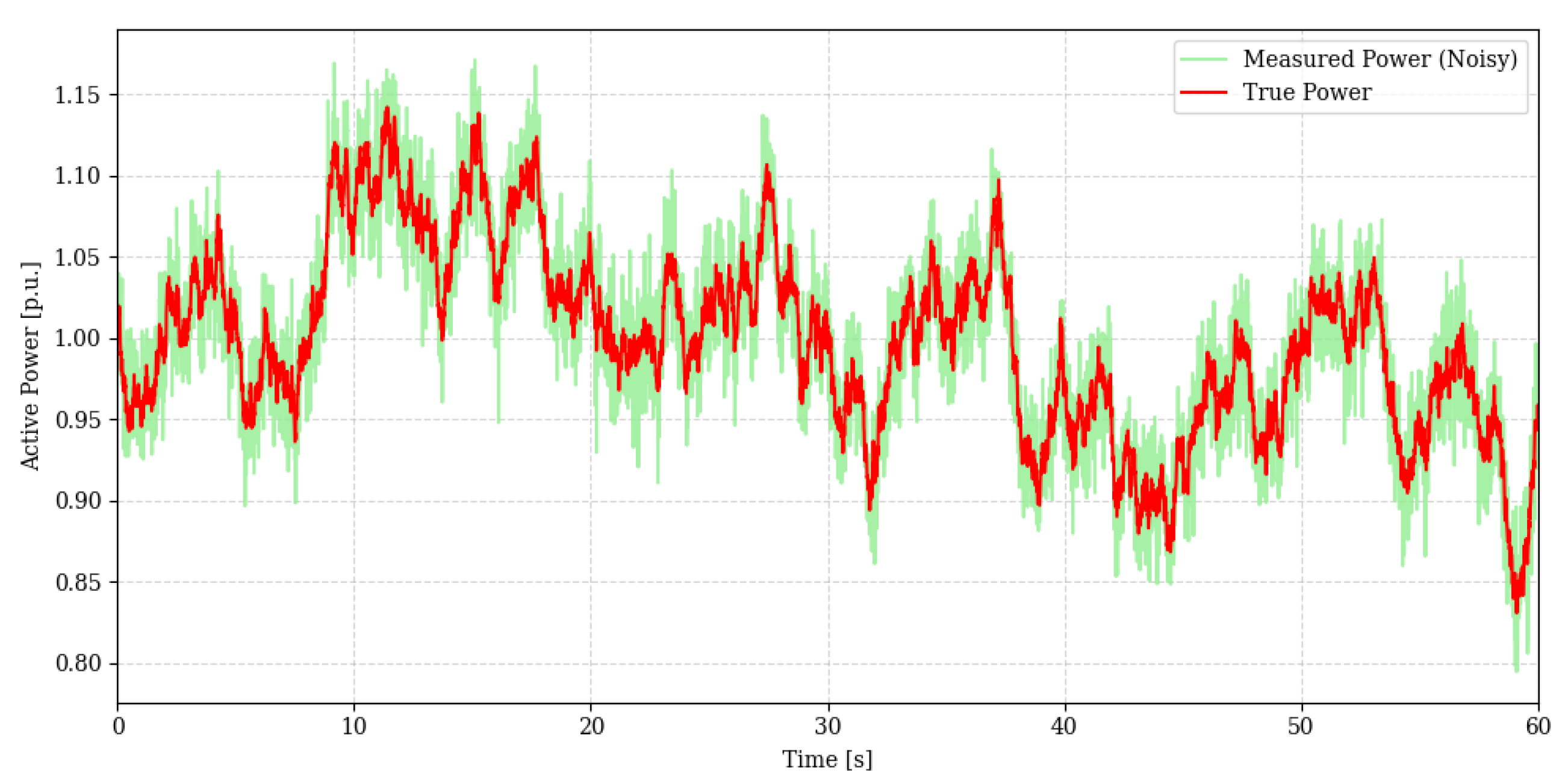
Here, we validate the effectiveness of the proposed data pre-processing strategy using SVMD. The simulation setup remains consistent with the stochastic load modeling described in Section 2, where the active power trajectory is driven by the OU process. As shown in Figure 9, the ground truth is depicted by the red curve, while the light green curve represents the measurement corrupted by Gaussian noise. This observation aligns with the analysis of noise-induced error accumulation presented in Section 4, particularly the signal enhancement mechanism detailed in Section 4.3. As discussed in the decentralized modeling part, such fluctuations are the root cause of the error accumulation in the decentralized scheme if left untreated. In the implementation of the SVMD algorithm, the penalty parameter $\alpha$ is set to 2000 to balance the bandwidth constraint and reconstruction fidelity, while the convergence tolerance $\gamma$ is set to ${10}^{-5}$ to ensure precise mode extraction.

To comprehensively validate the robustness of the SVMD-based denoising strategy against diverse measurement uncertainties, we evaluate its performance under both Gaussian and non-Gaussian noise conditions. Specifically, the Gaussian noise is modeled as $\mathcal{N}(0,{\sigma }^2)$ with a standard deviation of $\sigma =0.001$. To emulate skewed measurement anomalies, the non-Gaussian noise follows a Beta distribution $\mathcal{B}(2,5)$. To ensure a fair comparison, the raw Beta-distributed samples were centered to zero mean and scaled by a factor of approximately $6.26\times {10}^{-3}$ to strictly align their standard deviations with the Gaussian case.

The quantitative performance metrics are summarized in

Table 1. Denoising performance and computational efficiency comparison Under different noise profiles.

Noise Profile	Method	MAE	RMSE	Time (s)
Gaussian ($\sigma =0.001$)	Measured	0.02131	0.03152	-
	VMD	0.01645	0.02085	0.85
	SVMD	0.01601	0.02010	0.12
Beta ($\alpha =2,\beta =5$)	Measured	0.02542	0.03215	-
	SVMD	0.01724	0.02433	0.14

. It is evident that the proposed SVMD method significantly improves the data quality across both noise profiles. Under the Gaussian condition, SVMD reduces the mean absolute error (MAE) from 0.02131 to 0.01601 and the RMSE from 0.03152 to 0.02010. In the more challenging Beta noise scenario, the raw measurements exhibit higher initial distortion due to noise skewness; however, SVMD effectively suppresses these disturbances, reducing the MAE to 0.01724.

Finally, a comparative assessment against the standard VMD under the Gaussian profile highlights the superiority of the proposed approach. While VMD achieves comparable precision with an MAE of 0.01645, its concurrent mode extraction mechanism results in a significantly higher computational burden of 0.85 s. In contrast, SVMD leverages successive mode extraction and reduces the computation time to 0.12 s, which represents a speedup of approximately seven times compared to VMD, while the method maintains a slightly lower error rate. This enhanced computational efficiency combined with high accuracy makes SVMD a more favorable choice for online inertia estimation tasks.

7.3. Identification Accuracy and Posterior Analysis

To rigorously evaluate the MAP estimation performance of the proposed method, we conducted a comparative study involving the proposed PSIS framework and three benchmark techniques: the traditional IS method, the UKF-based method [12], and the PSO-based method [13]. To provide a granular view of the algorithmic robustness under diverse measurement uncertainties, the quantitative estimation results are analyzed under the two distinct noise profiles. Specifically, in the Bayesian inference setup, the proposal distribution is initialized as a Gaussian distribution centered at the nominal nameplate inertia, with variance set to 0.2 p.u. to represent the prior uncertainty.

Table 2. Comparison of parameter estimation errors under Gaussian noise ($\sigma =0.001$).

Parameter	Proposal Mean	True Value	Absolute Error (%)
			PSIS	UKF	PSO	IS
$H_1\left(s\right)$	60.0	57.0	2.04	2.25	2.10	2.32
$H_2\left(s\right)$	29.0	30.3	0.07	0.15	0.05	0.12
$H_3\left(s\right)$	34.0	35.8	5.50	5.35	5.65	5.55
$H_4\left(s\right)$	27.5	28.6	0.14	0.20	0.18	0.25
$H_5\left(s\right)$	24.5	26.0	0.08	0.12	0.20	0.10
$H_6\left(s\right)$	36.0	34.8	0.03	0.08	0.06	0.15
$H_{v1}\left(s\right)$	3.8	4.0	0.50	0.62	0.45	0.58
$H_{v2}\left(s\right)$	3.8	4.0	4.25	4.40	4.32	4.15
$H_{m1}\left(s\right)$	4.8	5.02	4.88	4.85	5.10	5.05
$H_{m2}\left(s\right)$	5.0	5.3	5.28	5.55	5.30	5.45

summarizes the estimation absolute errors under Gaussian noise. In this idealized scenario, all four algorithms demonstrate satisfactory performance with comparable estimation precision. Since the Gaussian noise assumption aligns with the theoretical foundations of UKF and the training environment of PSO, these benchmark methods yield results that are very close to those of the proposed PSIS framework. Although PSIS achieves the lowest absolute error rates in the majority of cases, the performance gap among the methods is marginal, indicating that conventional approaches are sufficient when measurement noise strictly follows a standard normal distribution.

However, the performance disparity becomes pronounced in the non-Gaussian scenario, as detailed in

Table 3. Comparison of parameter estimation errors under Beta noise ($\alpha =2,\beta =5$).

Parameter	Proposal Mean	True Value	Absolute Error (%)
			PSIS	IS	UKF	PSO
$H_1\left(s\right)$	60.0	57.0	2.18	2.56	6.85	7.45
$H_2\left(s\right)$	29.0	30.3	0.12	1.34	3.24	4.12
$H_3\left(s\right)$	34.0	35.8	5.76	6.12	9.45	10.12
$H_4\left(s\right)$	27.5	28.6	0.25	0.45	4.56	5.23
$H_5\left(s\right)$	24.5	26.0	0.15	1.89	3.78	4.45
$H_6\left(s\right)$	36.0	34.8	0.09	0.78	2.34	3.12
$H_{v1}\left(s\right)$	3.8	4.0	0.82	1.67	7.12	8.56
$H_{v2}\left(s\right)$	3.8	4.0	4.63	4.89	9.56	11.23
$H_{m1}\left(s\right)$	4.8	5.02	5.15	5.45	10.23	11.45
$H_{m2}\left(s\right)$	5.0	5.3	5.41	7.12	11.56	12.78

. Firstly, the proposed PSIS framework demonstrates superior performance, achieving the highest identification precision by effectively smoothing the tail distribution. The traditional IS method ranks second. In the presence of the heavy-tailed phenomenon induced by the Beta noise, IS’s particle-based nature allows it to capture the posterior shape better than rigid variance-based methods, although its accuracy is constrained by weight degeneracy. In contrast, the UKF and PSO methods exhibit the poorest performance. This is essentially because both approaches are predicated on the assumption that measurement errors follow a Gaussian distribution. Consequently, they fail to accommodate the asymmetric and heavy-tailed features of the posterior. Notably, while the maximum absolute errors of UKF and PSO rise to over 11% and 12%, respectively, the proposed PSIS maintains estimation errors at a level comparable to the Gaussian case, validating its remarkable resilience under complex real-world ambient measurements.

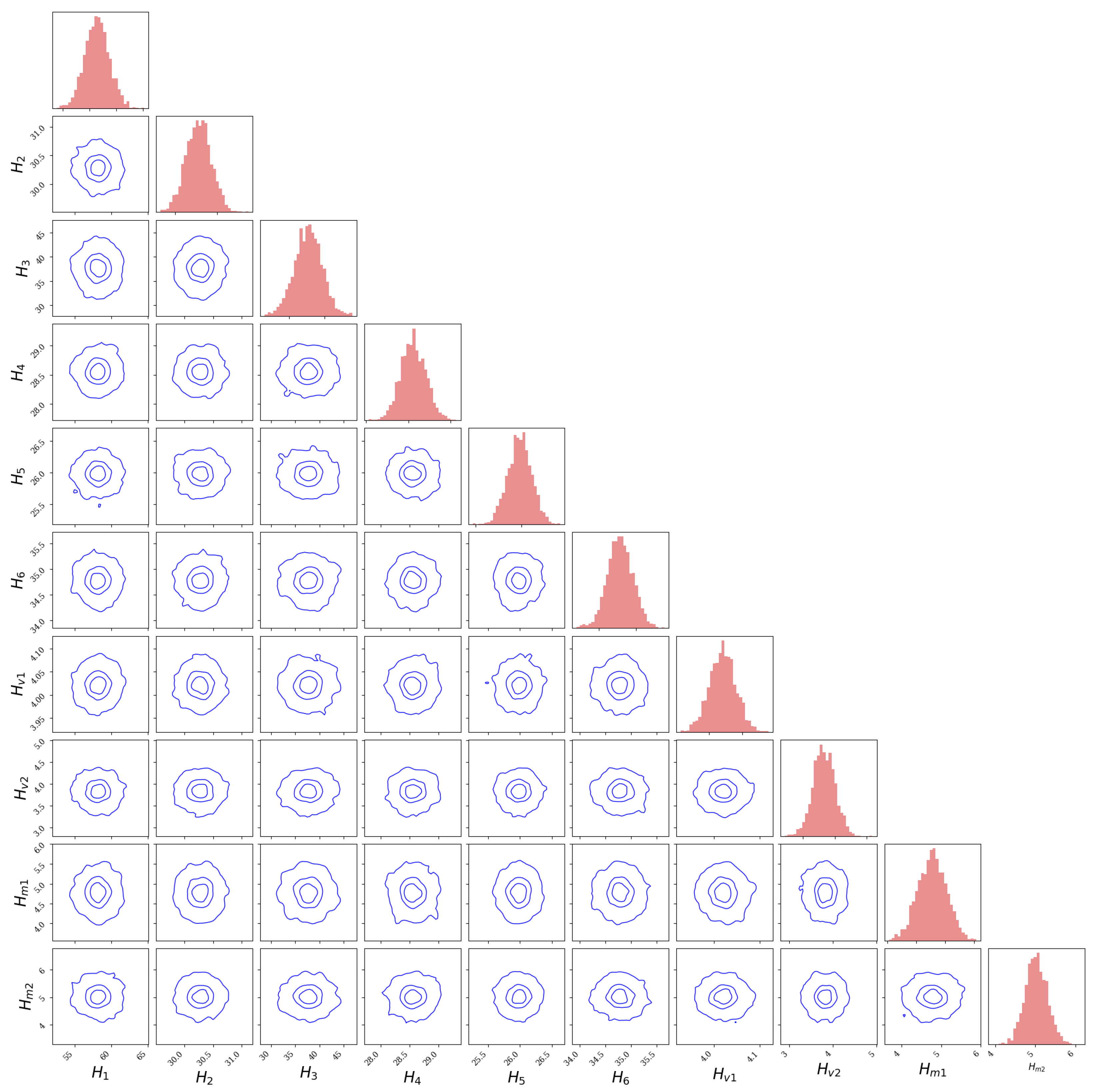
Furthermore, to visualize the uncertainty and correlations of the estimated parameters, the posterior distributions obtained via the PSIS method are depicted in Figure 10. This corner plot illustrates the 1D marginal distributions on the diagonal and the 2D joint posterior densities on the off-diagonal elements. It can be seen that the probability mass of the samples is tightly concentrated around the true values (indicated by the high-density regions), which validates the convergence of the proposed algorithm. The 95% confidence intervals shown in the contour plots confirm that the method successfully captures the true system dynamics, even under stochastic ambient excitations. Overall, the combination of low estimation errors and well-defined posterior distributions underscores the effectiveness and accuracy of the proposed decentralized framework in identifying key dynamic parameters in modern power systems.

7.4. Robustness and Scalability Analysis

To rigorously evaluate the robustness of the proposed framework against the quality of prior knowledge, we conducted a sensitivity analysis regarding the proposal distribution. Specifically, a comparative study was performed between the proposed PSIS framework and the traditional IS method. In this analysis, the variance of the proposal distributions was maintained at 0.2 p.u., consistent with the previous section, while the initial means were intentionally adjusted to deviate from the true values. We established three distinct scenarios to mimic varying levels of prior accuracy: Case I represents a small deviation of approximately 2.5%, Case II represents a medium deviation of roughly 15%, and Case III represents a large deviation of about 40%. Representative parameters $H_1$, $H_{v1}$, and $H_{m1}$ are selected to demonstrate the performance trends. The quantitative estimation results are summarized in

Table 4. Comparison of estimation errors under different proposal mean deviations with fixed variance.

Parameter	True Value	Prop. Mean	Abs. Error %
			PSIS	IS
Case I: Small Deviation ∼2.5%
$H_1$ [s]	57.0	58.5	0.45	1.12
$H_{v1}$ [s]	4.0	4.1	0.21	0.89
$H_{m1}$ [s]	5.02	5.15	0.33	0.95
Case II: Medium Deviation ∼15%
$H_1$ [s]	57.0	65.5	2.18	5.67
$H_{v1}$ [s]	4.0	4.6	1.85	6.23
$H_{m1}$ [s]	5.02	5.77	2.41	6.89
Case III: Large Deviation ∼40%
$H_1$ [s]	57.0	79.8	5.24	21.35
$H_{v1}$ [s]	4.0	5.6	4.65	25.12
$H_{m1}$ [s]	5.02	7.03	5.82	28.45

.

As evidenced by the results in Table 4, the accuracy of the traditional IS method deteriorates significantly as the proposal mean deviates further from the true value. In Case III, where the initial guess is far from the ground truth with a 40% deviation, the IS method suffers from severe weight degeneracy and results in estimation errors exceeding 20%. In sharp contrast, the proposed PSIS framework demonstrates remarkable resilience. Even under large initial deviations, PSIS effectively mitigates the variance of importance weights through Pareto smoothing and maintains the estimation error at a low level of around 5%. Furthermore, it is noteworthy that, even in Case I, where the proposal distribution is reasonably accurate, PSIS still exhibits a distinct precision advantage over IS. These findings confirm that the proposed method is robust against poor prior knowledge and consistently outperforms the benchmark method across varying degrees of initialization uncertainty.

In addition to robustness, the scalability of the estimation framework against the dimension of the parameter space is a critical criterion. High-dimensional identification scenarios, common in modern grids with the high-density integration of renewables, pose significant computational challenges. To evaluate the computational efficiency of the proposed method under varying identification dimensions, we conducted a scalability test by adjusting the number of generation units involved, thereby directly manipulating the total number of unknown parameters. The high-dimensional scenario comprising six SGs, two GFLs, and two GFMs, totaling 10 units, served as the baseline. We created two lower-dimensional scenarios by selectively decreasing the number of units to seven and four. For comparison, a traditional centralized Bayesian inference method that estimates all unknown parameters simultaneously using a global measurement vector was employed as a benchmark. Both the proposed decentralized method and the centralized benchmark were executed under identical stopping conditions and terminated once 20,000 valid posterior samples were collected.

The computation times for both methods across different identification dimensions are recorded in

Table 5. Computation time comparison between decentralized and centralized schemes under different identification dimensions.

Scenario	Composition	Computation Time/s
		Proposed Dec.	Centralized
Case I (4 Units)	2 SG, 1 GFL, 1 GFM	24.5	156.2
Case II (7 Units)	4 SG, 1 GFL, 2 GFM	42.3	824.6
Case III (10 Units)	6 SG, 2 GFL, 2 GFM	61.8	2352.4

. As anticipated, the computational cost of the centralized method exhibits an explosive growth trend as the parameter dimension increases. Due to the curse of dimensionality, the search space expands exponentially, causing the time consumption of the centralized approach to grow roughly cubically. In the high-dimensional scenario denoted as Case III, the centralized method requires over 39 min or 2352.4 s to converge, rendering it impractical for online applications. In sharp contrast, the proposed decentralized framework demonstrates excellent scalability with near-linear time complexity. By decoupling the high-dimensional problem into independent low-dimensional sub-problems, the proposed method keeps the local identification dimension low and completes the estimation for the most complex scenario in merely 61.8 s. This significant speedup confirms that the decentralized architecture effectively breaks through the computational bottleneck and makes it highly suitable for high-dimensional parameter identification tasks.

7.5. Inertia Estimation for IEEE 118-Bus System

To further demonstrate the generalizability and scalability of the proposed framework, we extended the validation to the larger IEEE 118-bus test system. This system represents a more complex network topology typical of real-world power grids, comprising 118 buses, 54 generators, and 186 branches. In this case study, to emulate a modern grid scenario with high renewable penetration, we modified the standard benchmark by replacing the synchronous generators at buses 15, 18, 19, and 24 with grid-forming converters. The inertia and virtual inertia constants of the first ten generation units in the system were selected as the targets for identification.

Consistent with the experimental setup in the previous subsections, the prior parameter uncertainty was maintained at 10% and the ambient load fluctuations were modeled as Gaussian noise. The estimation results are summarized in

Table 6. Estimation results for the modified IEEE 118-bus system.

Unit Index	Bus No.	Type	True Value/s	Estimation Results
				MAP Value/s	Error/%
1	10	SG	5.00	5.04	0.80
2	12	SG	4.50	4.47	0.67
3	15	GFM	6.00	6.02	0.33
4	18	GFM	6.00	5.96	0.67
5	19	GFM	6.00	6.05	0.83
6	24	GFM	6.00	5.98	0.33
7	25	SG	3.50	3.53	0.86
8	26	SG	4.00	3.97	0.75
9	27	SG	3.80	3.82	0.53
10	31	SG	3.20	3.18	0.62

. It can be observed that the proposed decentralized Bayesian inference method achieves high precision across all identified units, with the maximum relative error remaining below 1.5%. Furthermore, regarding computational efficiency, the entire identification process for the IEEE 118-bus system was completed in 75.4 s. Compared to the 61.8 s required for the IEEE 39-bus system in Case III, the computation time did not exhibit an explosive increase, despite the significant expansion in system scale from 39 to 118 buses. These results collectively confirm that the proposed algorithm is not limited to small-scale systems but is also capable of achieving accurate and efficient inertia estimation in large-scale power networks, effectively validating the scalability of the decentralized scheme.

8. Conclusions and Future Work

This paper presents a robust, decentralized framework for the dynamic parameter identification of modern power systems characterized by heterogeneous generation resources. By addressing the critical challenges of parameter coupling, ambient noise accumulation, and probabilistic computational instability, the proposed methodology offers a viable solution for routine system monitoring using ubiquitous PMU data. Specifically, the application of trajectory sensitivity analysis provides a quantitative criterion for distinguishing dominant inertia parameters from insensitive control gains. This screening mechanism ensures that the identification process remains physically meaningful and computationally efficient, effectively preventing over-parameterization issues as seen in complex hybrid networks.

Furthermore, the integration of successive variational mode decomposition (SVMD) and Pareto smoothed importance sampling (PSIS) significantly enhances the robustness of the identification process. The SVMD technique effectively extracts electromechanical dynamic modes from noisy ambient measurements, mitigating the error accumulation phenomenon inherent in decentralized playback schemes and reducing the mean absolute error (MAE) of input signals from 0.0213 to 0.0160. Building on these high-quality data, the PSIS algorithm overcomes the weight degeneracy limitations of standard particle filters. The simulation results obtained on the modified IEEE 39-bus system demonstrate that the framework achieves high-precision estimation for both synchronous and virtual inertia, with relative errors maintained below 5.50%, while providing reliable uncertainty quantification through well-defined posterior distributions.

Future work will focus on enhancing the framework’s robustness against complex measurement anomalies, specifically addressing challenges like data dropouts and gross errors. To mitigate these non-ideal conditions, we intend to integrate robust statistical techniques, such as Huber loss functions or M-estimators, into the Bayesian inference process to ensure reliable identification under severe data quality degradation.

References

1. Chow, J.H. Enabling Inverter-based Resource Stability Control in Power Systems with High Renewable Penetration. CSEE J. Power Energy Syst. 2023, 9, 1248–1250. [Google Scholar] [CrossRef] [Scilit]
2. Li, J.; Zhang, H. Two-Stage Optimization Research of Power System with Wind Power Considering Energy Storage Peak Regulation and Frequency Regulation Function. Energies 2025, 18, 4947. [Google Scholar] [CrossRef] [Scilit]
3. Kosterev, D.; Taylor, C.; Mittelstadt, W. Model validation for the August 10, 1996 WSCC system outage. IEEE Trans. Power Syst. 1999, 14, 967–979. [Google Scholar] [CrossRef] [Scilit]
4. Waskito, F.; Wijaya, F.D.; Firmansyah, E. Review of Virtual Inertia Based on Synchronous Generator Characteristic Emulation in Renewable Energy-Dominated Power Systems. Electricity 2025, 6, 69. [Google Scholar] [CrossRef] [Scilit]
5. Cheng, M.; Yu, J.; Wu, M.; Zhang, Y.; Zhu, Y.; Zhu, Y. Transient Stability Analysis of Wind-Integrated Power Systems via a Kuramoto-like Model Incorporating Node Importance. Energies 2025, 18, 3277. [Google Scholar] [CrossRef] [Scilit]
6. Zeng, J.; Li, X.; Dai, H.; Zhang, L.; Wang, W.; Zhang, Z.; Kong, S.; Xu, L. A Residual Physics-Informed Neural Network Approach for Identifying Dynamic Parameters in Swing Equation-Based Power Systems. Energies 2025, 18, 2888. [Google Scholar] [CrossRef] [Scilit]
7. Gotti, D.; Bizzarri, F.; Brambilla, A.; Giudice, D.d.; Grillo, S.; Linaro, D.; Ledesma, P.; Amaris, H. Inertia Estimation of a Power System Area Based on Iterative Equation Error System Identification. IEEE Trans. Power Syst. 2024, 39, 6469–6481. [Google Scholar] [CrossRef] [Scilit]
8. Liu, K.; Xu, Y.; Gu, W.; Ge, J.; Lu, S.; Mili, L.; Shen, C. A Bayesian Approach for Online Inertia Estimation of Synchronous and Nonsynchronous Generators. IEEE Trans. Instrum. Meas. 2024, 73, 1006012. [Google Scholar] [CrossRef] [Scilit]
9. Wang, S.; Sun, Z. An Energy-Function-Based Approach for Power System Inertia Assessment. Energies 2025, 18, 3105. [Google Scholar] [CrossRef] [Scilit]
10. Huang, Z.; Du, P.; Kosterev, D.; Yang, S. Generator dynamic model validation and parameter calibration using phasor measurements at the point of connection. IEEE Trans. Power Syst. 2013, 28, 1939–1949. [Google Scholar] [CrossRef] [Scilit]
11. Helac, V.; Renner, H.; Hanjalic, S. Wind Power Plant’s Synthetic Inertia Estimation Using Extended Kalman Filter. Eng. Proc. 2024, 60, 4. [Google Scholar] [CrossRef] [Scilit]
12. Tan, B.; Zhao, J. Data-Driven Adaptive Unscented Kalman Filter for Time-Varying Inertia and Damping Estimation of Utility-Scale IBRs Considering Current Limiter. IEEE Trans. Power Syst. 2024, 39, 7331–7345. [Google Scholar] [CrossRef] [Scilit]
13. Zhou, S.; Wang, D.; Ni, Y.; Song, K.; Li, Y. Improved Particle Swarm Optimization for Parameter Identification of Permanent Magnet Synchronous Motor. Comput. Mater. Contin. 2024, 79, 2187–2207. [Google Scholar] [CrossRef] [Scilit]
14. Chassin, D.; Huang, Z.; Donnelly, M.; Hassler, C.; Ramirez, E.; Ray, C. Estimation of WECC system inertia using observed frequency transients. IEEE Trans. Power Syst. 2005, 20, 1190–1192. [Google Scholar] [CrossRef] [Scilit]
15. Ashton, P.M.; Saunders, C.S.; Taylor, G.A.; Carter, A.M.; Bradley, M.E. Inertia Estimation of the GB Power System Using Synchrophasor Measurements. IEEE Trans. Power Syst. 2015, 30, 701–709. [Google Scholar] [CrossRef] [Scilit]
16. Phurailatpam, C.; Rather, Z.H.; Bahrani, B.; Doolla, S. Measurement-Based Estimation of Inertia in AC Microgrids. IEEE Trans. Sustain. Energy 2020, 11, 1975–1984. [Google Scholar] [CrossRef] [Scilit]
17. Schiffer, J.; Aristidou, P.; Ortega, R. Online Estimation of Power System Inertia Using Dynamic Regressor Extension and Mixing. IEEE Trans. Power Syst. 2019, 34, 4993–5001. [Google Scholar] [CrossRef] [Scilit]
18. Liu, K.; Xu, Y.; Zheng, Z.; Yao, Y.; Gu, W.; Liu, C.; Lu, S.; Mili, L.; Shi, C. Decentralized Bayesian Inference for Inertia Estimation in Modern Power System Using Ambient Measurements. IEEE Trans. Power Syst. 2025, 40, 5354–5368. [Google Scholar] [CrossRef] [Scilit]
19. Tuttelberg, K.; Kilter, J.; Wilson, D.; Uhlen, K. Estimation of Power System Inertia from Ambient Wide Area Measurements. In Proceedings of the 2019 IEEE Power & Energy Society General Meeting (PESGM), Atlanta, GA, USA, 4–8 August 2019. [Google Scholar] [CrossRef] [Scilit]
20. Guo, J.; Wang, X.; Ooi, B.T. Estimation of Inertia for Synchronous and Non-Synchronous Generators Based on Ambient Measurements. IEEE Trans. Power Syst. 2022, 37, 3747–3757. [Google Scholar] [CrossRef] [Scilit]
21. Bizzarri, F.; Giudice, D.d.; Grillo, S.; Linaro, D.; Brambilla, A.; Milano, F. Inertia Estimation Through Covariance Matrix. IEEE Trans. Power Syst. 2024, 39, 947–956. [Google Scholar] [CrossRef] [Scilit]
22. Poudyal, A.; Fourney, R.; Tonkoski, R.; Hansen, T.M.; Tamrakar, U.; Trevizan, R.D. Convolutional Neural Network-based Inertia Estimation using Local Frequency Measurements. In Proceedings of the 2020 52nd North American Power Symposium (NAPS), Tempe, AZ, USA, 11–13 April 2021; pp. 1–6. [Google Scholar] [CrossRef] [Scilit]
23. Sauer, P.; Pai, M.; Chow, J. Power System Dynamics and Stability: With Synchrophasor Measurement and Power System Toolbox, 2nd ed.; Wiley Press: Hoboken, NJ, USA, 2017. [Google Scholar] [CrossRef] [Scilit]
24. Shen, C.; Shuai, Z.; Shen, Y.; Peng, Y.; Liu, X.; Li, Z.; Shen, Z.J. Transient Stability and Current Injection Design of Paralleled Current-Controlled VSCs and Virtual Synchronous Generators. IEEE Trans. Smart Grid 2021, 12, 1118–1134. [Google Scholar] [CrossRef] [Scilit]
25. Mele, F.M.; Zárate-Miñano, R.; Milano, F. Modeling Load Stochastic Jumps for Power Systems Dynamic Analysis. IEEE Trans. Power Syst. 2019, 34, 5087–5090. [Google Scholar] [CrossRef] [Scilit]
26. Konishi, T.; Kubo, T.; Watanabe, K.; Ikeda, K. Variational Bayesian Inference Algorithms for Infinite Relational Model of Network Data. IEEE Trans. Neural Netw. Learn. Syst. 2015, 26, 2176–2181. [Google Scholar] [CrossRef] [Scilit]
27. Akhlaghi, S.; Jordan, S. Trajectory Sensitivity Analysis of Composite Load Model with Aggregated Distributed Energy Resource. In Proceedings of the 2021 IEEE Power & Energy Society General Meeting (PESGM), Washington, DC, USA, 26–29 July 2021; pp. 1–5. [Google Scholar] [CrossRef] [Scilit]
28. Wang, S.; Zhao, J.; Huang, Z.; Diao, R. Assessing Gaussian Assumption of PMU Measurement Error Using Field Data. IEEE Trans. Power Deliv. 2018, 33, 3233–3236. [Google Scholar] [CrossRef] [Scilit]
29. Varghese, A.C.; Pal, A.; Dasarathy, G. Transmission Line Parameter Estimation Under Non-Gaussian Measurement Noise. IEEE Trans. Power Syst. 2023, 38, 3147–3162. [Google Scholar] [CrossRef] [Scilit]
30. Vehtari, A.; Simpson, D.; Gelman, A.; Yao, Y.; Gabry, J. Pareto smoothed importance sampling. J. Mach. Learn. Res. 2024, 25, 1–58. [Google Scholar]
Figure 3. Schematic illustration of the signal enhancement process: (a) the original noisy voltage measurement and (b) the reconstructed signal after applying SVMD denoising.
Energies 19 00823 g003
Figure 4. Illustration of the weight degeneracy phenomenon in importance sampling due to distribution mismatch. The vertical dashed orange lines mark the locations of the two peaks of the target distribution.
Energies 19 00823 g004
Figure 5. Topology of the modified IEEE 39-bus system featuring heterogeneous generation resources, including 6 SGs, 2 GFMs, and 2 GFL converters.
Energies 19 00823 g005
Figure 6. Relative trajectory sensitivity comparison of SG parameters: H , D , X d .
Energies 19 00823 g006
Figure 7. Relative trajectory sensitivity comparison of GFM parameters: H m , D q , K .
Energies 19 00823 g007
Figure 8. Relative trajectory sensitivity comparison of GFL parameters: H v , T v , T p .
Energies 19 00823 g008
Figure 9. Comparative visualization of the noise-free system response (red line) vs. the corrupted PMU measurements (green line) under stochastic ambient excitation, serving as the baseline for evaluating the subsequent SVMD denoising performance.
Energies 19 00823 g009
Figure 10. Visualization of the identified 10-dimensional posterior distributions for inertia parameters ( H , H m , H v ) in the modified IEEE 39-bus system under stochastic ambient excitation. The diagonal subplots present the marginal histograms of each parameter, confirming the convergence of the PSIS estimator toward the true values. The off-diagonal subplots display the bivariate density contours with 95% confidence regions, illustrating the statistical correlations between different generator units and the robustness of the probabilistic inference against non-Gaussian measurement noise.
Energies 19 00823 g010