A Priori Study of Inter-Scale Kinetic Energy Transfer and Energy Exchange in a Turbulent Premixed Flame

Abstract

Velocity, pressure, and density fields computed in earlier three-dimensional direct numerical simulations of a statistically stationary, planar, one-dimensional, low-Mach-number hydrogen–air flame propagating in small-scale, moderately intense, spatially decaying turbulence are filtered out using top-hat filters of four different widths. Certain source/sink filtered terms in the transport equations for resolved and subfilter-scale kinetic energies are analyzed. These are (i) the rate of inertial transfer of kinetic energy between resolved and subfilter scales, (ii) baropycnal work, (iii) subfilter-scale velocity–pressure–gradient term, and (iv) subfilter-scale pressure–dilatation term. These filtered terms are averaged over transverse planes and time or conditioned to the filtered combustion progress variable. Results show that terms (i) and (ii) work to transfer kinetic energy from smaller to larger scales (backscatter) and from larger to smaller scales, respectively, with the baropycnal work dominating the former term. These trends are observed for mean and conditional terms. The mean velocity–pressure–gradient term is positive and works to increase subfilter-scale kinetic energy due to combustion-induced thermal expansion. The pressure–dilatation term changes its sign from negative to positive at the leading and trailing edges, respectively, of the turbulent flame brush. Under conditions of the present study, the magnitudes of the mean velocity–pressure–gradient and pressure–dilatation terms are smaller when compared to the baropycnal work. Probability Density Functions (PDFs) for the explored filtered terms exhibit long tails, are highly skewed, and are characterized by a large kurtosis, thus implying significant intermittency of inter-scale energy transfer and energy exchange between internal and kinetic energy in the flame. These PDFs indicate that the intermittency of the inter-scale energy transfer and energy exchange depends substantially on mechanisms and scales of energy injection.

1. Introduction

According to the classical statistical theory of locally isotropic and homogeneous turbulence in incompressible flows [1,2,3], turbulent kinetic energy is transferred on average from large scales, where it is generated, to small scales via the turbulence cascade [4,5], with the energy flux being conserved in the inertial range of scales, but the energy being dissipated due to molecular viscosity at the smallest scales. However, the modern picture of inter-scale turbulence energy transfer substantially expands this classical paradigm of energy cascade by going beyond the statistical average framework. For instance, the local behavior of turbulent kinetic energy transfer is known to be highly intermittent in space and time, i.e., there are significant spatial-temporal fluctuations of the inter-scale energy transfer rate [6,7,8,9,10,11,12,13,14,15,16,17,18,19]. Specifically, there are localized regions with inverse energy cascade, i.e., from small scales to large scales. This phenomenon is often referred to as backscatter. The net average cascade is a result of downscale/direct and upscale/backscatter energy transfer. Even if the classical forward cascade statistically overwhelms backscatter in many turbulent flows [7,20,21,22], analysis of inter-scale kinetic energy transfer was in the focus of numerous studies reviewed elsewhere [5]. Their results indicate that inter-scale kinetic energy transfer is sufficiently well understood in the classical case of incompressible, homogeneous, isotropic turbulence.

In compressible (with large density variations), homogeneous, non-reacting and reacting turbulence, the physical picture is more intricate due to the appearance of two new physical mechanisms [23,24,25,26,27,28,29,30,31,32,33], which are absent in incompressible turbulence. First, baroclinic effects, which arise from misalignment of pressure and density gradients, induce extra inter-scale kinetic energy transfer supplementary to the inertial Kolmogorov cascade [23,24,25,28]. Contrary to the inter-scale energy transfer in incompressible turbulence, controlled by the solenoidal motion (via the vorticity stretching mechanism), the baroclinity-induced transfer arises due to density variations and, therefore, as can be inferred, is associated with the dilatational component of the velocity vector. Second, velocity–pressure–gradient work (associated often with the pressure–dilatation term in a transport equation for internal energy) causes energy exchange between kinetic and internal energies. This energy exchange is also associated with the dilatational component of the velocity vector and proceeds directly at any given scale, thus breaking conservation of the inter-scale kinetic energy flux in the inertial range of scales. Therefore, energy exchange between kinetic and internal energies may significantly impact inter-scale kinetic energy transfer [26,27,31,32].

Furthermore, it should be stressed that the mean velocity divergence vanishes, i.e., the mean density is constant, in statistically homogeneous (both non-reacting and reacting) compressible turbulence. This occurs even if local velocity divergence can take both positive and negative values, because the Probability Density Function (PDF) for the velocity divergence is almost symmetrical with respect to zero. On the contrary, in inhomogeneous mean turbulent flows, asymmetry of the PDF shape may be well pronounced and the mean velocity divergence may be significant [34,35]. For instance, expansion zones induced by heat release in premixed flames are characterized by positive local dilatation, make the mean flow highly inhomogeneous, and result in a strong bias of pressure–dilatation work to positive values. Accordingly, inter-scale energy transfer in flames is substantially affected by this work, contrary to the case of a homogeneous turbulent flow.

As reviewed elsewhere [36,37,38], in a typical premixed turbulent flame, heat release, density variations, dilatation, and chemical reactions are localized to spatial zones whose scales are comparable with laminar flame thickness, which is well below 1 mm under atmospheric conditions. These scales are substantially smaller than scales of large turbulent eddies, but are often larger than or comparable with the Kolmogorov length scale. Heat release in these zones induces pressure–dilatation work, with a small part of this work resulting in the local injection of kinetic energy to the flow at small scales or, in other words, the conversion of internal energy to kinetic energy. Therefore, in a general case, injection of kinetic energy in a premixed flame may occur not only at large scales, e.g., if large-scale forcing is applied in numerical simulations [39,40] or the flame is stabilized in a turbulent shear flow [41,42], but also at small scales due to the conversion of internal energy to kinetic energy. On the contrary, in incompressible turbulence, kinetic energy is typically injected at large scales only.

Conversion of internal energy to kinetic energy at small scales can result in backscatter. Indeed, over the past decade, the phenomenon of combustion-induced backscatter was explored by several research groups by analyzing both data computed in Direct Numerical Simulation (DNS) studies of premixed turbulent flames in simple flow configurations [39,40,43,44,45,46,47,48,49,50] and experimental data obtained from swirled flames [41,42]. It is worth noting, however, that compressibility effects, i.e., significant variations in pressure and density, can dominate the influence of combustion dynamics on dilatation and backscatter in high-speed flows, as found in an a priori DNS study of the dynamics of backscatter of kinetic energy in inert and reacting supersonic (Mach number is larger than 2) hydrogen–air turbulent mixing layers [51].

Moreover, in premixed flames, the mean dilatation is not only positive, contrary to a typical non-reacting compressible flow, but is also sufficiently large when compared to velocity gradients in the incoming turbulence. The former peculiarity (positive mean dilatation rate) of premixed turbulent flames when compared to compressible non-reacting turbulence (where dilatation rate vanishes after averaging) can have a strong impact on the intermittency of the inter-scale energy transfer. For instance, injection of kinetic energy and energy exchange are strongly influenced by pressure–dilatation terms in transport equations for the internal and kinetic energies; see Equations (1) and (3), respectively, in the next section.

However, the influence of strong heat release localized to thin premixed flames on intermittency of inter-scale energy transfer was beyond the focus of research into both turbulence and combustion. For instance, the most common approaches to studying intermittency of inter-scale energy transfer [2,3,52] deal either with a PDF of a quantity relevant to the transfer or with images of iso-surfaces of sub-filter scale (sfs) flux. However, the present authors are not aware of the applications of any of these two major diagnostic techniques to analyzing data obtained from a premixed flame.

Accordingly, the present work aims at bridging this knowledge gap by applying a filtering approach and PDF techniques to a priori analyzing unsteady, three-dimensional (3D) DNS data obtained by Dave et al. [53,54] from a statistically stationary, planar, and one-dimensional, low-Mach-number, complex-chemistry lean hydrogen–air flame propagating in moderately intense, small-scale, and spatially decaying (upstream of the flame) turbulence in a box. The choice of this configuration (specifically, statistically stationary turbulence decaying in the direction normal to the mean flame upstream of it, but homogeneous in each cross section) offers the opportunity to explore a “pure” case associated solely with injection of kinetic energy at small scales due to the lack of injection of kinetic energy at large scales. These DNS data were already analyzed by us either by directly averaging them over transverse planes and time (see Refs. [55,56] and papers cited therein) or by filtering them, followed by time- and transverse averaging [57,58]. In the present work, intermittency of inter-scale energy transfer and of energy exchange between internal and kinetic energy is investigated by spatially filtering the raw DNS data, followed by calculating various PDFs and their moments by processing unsteady, three-dimensional filtered fields of velocity, density, pressure, and their spatial gradients. It is worth stressing that the study goals are restricted to exploring phenomena that (i) are specific to flames when compared to incompressible or compressible, statistically homogeneous or inhomogeneous, reacting or non-reacting turbulent flows characterized by negligible mean dilatation and (ii) should be taken into account when running Large Eddy Simulations (LESs) of premixed turbulent flames by adopting and/or extending models well established in LES research into other turbulent flows [59,60,61,62]. Validation or development of models for LES research into premixed turbulent combustion is beyond the scope of the present work.

In the next section, the DNS attributes and applied numerical diagnostic techniques are summarized. Numerical results are reported and discussed in Section 3, followed by conclusions.

2. DNS Attributes and Data Analysis

2.1. DNS Data

The DNS data were obtained from an unconfined, statistically one-dimensional and planar, lean (the equivalence ratio $\varphi =0.81$) and slightly preheated (unburned gas temperature $T_u=310$ K) H₂-air flame propagating in a box ($19.18\times 4.8\times 4.8$ mm) meshed using a uniform grid of $960\times 240\times 240$ cells [53,54]. The simulations were performed adopting an open-access PENCIL code [63], the mixture-averaged transport model implemented into it, and a detailed chemical mechanism (21 reactions, 9 species) by Li et al. [64]. The laminar flame speed $S_L=1.84$ m/s, thickness ${\delta }_L=(T_b-T_u)/max\left\{\right|\nabla T\left|\right\}=0.36$ mm, and time scale ${\tau }_f={\delta }_L/S_L=0.20$ ms, where subscripts u and b designate unburned and burned mixtures, respectively. The achieved numerical resolution (18 grid points per laminar flame thickness) is comparable with resolution adopted in the state-of-the-art DNS studies of complex-chemistry premixed turbulent flames, e.g., the grid step $\Delta x={\delta }_L/19$ or ${\delta }_L/16$ in Ref. [65] or [66], respectively.

Homogeneous isotropic turbulence was pre-generated using forcing at low wavenumbers in a separate cube with the fully periodic boundary conditions [53]. The generation process was performed until a statistically stationary stage was reached. The obtained turbulence displays the Kolmogorov-Obukhov −5/3 spectrum [2,3] and is characterized by the root-mean-square (rms) velocity $u^{\prime }=6.7$ m/s, integral length scale $L=3.1$ mm or $L=8.6{\delta }_L$, turbulent Reynolds number $R{e}_t=u^{\prime }L/{\nu }_u=950$, Kolmogorov length scale ${\eta }_K={({\nu }_u^3/\langle \epsilon \rangle )}^{1/4}=0.018$ mm, integral and Kolmogorov time scales ${\tau }_t=L/u^{\prime }=0.46$ ms and ${\tau }_K={({\nu }_u/\langle \epsilon \rangle )}^{1/2}=0.015$ ms, respectively. Here, $\langle \epsilon \rangle =2{\nu }_u{S}_{ij}{S}_{ij}$ designates the rate of dissipation of turbulent kinetic energy, averaged over the cube; $\nu$ is kinematic viscosity; $S_{ij}=0.5(\partial u_i/\partial x_j+\partial u_j/\partial x_i)$ is the rate-of-strain tensor; $u_i$ is i-th component of velocity vector; and the Einstein summation convention applies to repeated indexes. Accordingly, $\Delta x\approx {\eta }_K$ (cf. with $\Delta x\approx 2{\eta }_K$ in Ref. [66] or even larger in Ref. [65]), the Damköhler number $Da={\tau }_t/{\tau }_f=2.35$ and the number ${({\delta }_L/{\eta }_K)}^2$, which is sometimes associated with the Karlovitz number, is as large as 400. Note, that a more appropriate Karlovitz number $Ka={\tau }_f/{\tau }_K=13$ is significantly smaller, because $S_L{\delta }_L\gg {\nu }_u$ in lean H₂-air flames [67], but $Ka=13$ is still substantially larger than unity.

When running combustion simulations, the pre-generated turbulence was injected into the computational domain through the left boundary at a constant mean inlet velocity, which was not changed during the simulations. Subsequently, the injected turbulence decayed along the mean flow direction x (symmetry boundary conditions were set at transverse boundaries). Accordingly, $u^{\prime }=3.3$ m/s and $Ka=3.3$ at the leading edge of the mean flame brush, associated with the transverse-averaged value of the fuel-based combustion progress variable c equal to 0.01. Nevertheless, the turbulence length scales evaluated at the inlet boundary and at the leading edge are roughly equal, i.e., ${({\delta }_L/{\eta }_K)}^2$ is still about 400 at the leading edge. Here, $c(\mathit{x},t)=(Y_F(\mathit{x},t)-Y_{F,u})/(Y_{F,b}-Y_{F,u})$ is defined using the fuel mass fraction $Y_F$ to satisfy a constraint of $0\le c(\mathit{x},t)\le 1$, whereas local values of temperature-based combustion progress variable can be larger than unity due to differences in molecular diffusivities of heat, H₂, and O₂ [68,69].

Based on the reported values of $Ka$ and, especially, ${({\delta }_L/{\eta }_K)}^2$, the studied flame might be associated with a highly turbulent regime of premixed burning, called “stirred reactors”, “thickened flames”, or “broken reaction zones” in combustion regime diagrams invented by Williams [70], Borghi [71], and Peters [72], respectively, by considering single-step-chemistry equidiffusive flames, where $Ka={\tau }_f/{\tau }_K={({\delta }_L/{\eta }_K)}^2$. However, previous analyses [55,56] of these complex-chemistry DNS data showed that local flames statistically retained the structure of the unperturbed laminar flame. Therefore, the studied case is better associated with the flamelet combustion regime [70,71,72], in line with numerous other recent experimental and DNS data reviewed elsewhere [36,37,38], which indicate that turbulent combustion can occur in the flamelet regime at Karlovitz numbers significantly larger than unity.

It is also worth noting that the thin reaction zone regime introduced by Peters [72] does not seem to be relevant to complex-chemistry near-stoichiometric or moderately lean H₂-air flames, because thicknesses of preheat and reaction zones are comparable in such flames [67]. Moreover, a distributed burning regime is associated with $Ka\gg 1$ has probably only been achieved in a few DNS studies [65,66]. Furthermore, differential diffusion effects, which play an important role in turbulent burning of lean H₂-containing mixtures, as reviewed elsewhere [68,73,74], are weakly pronounced in the investigated turbulent flame [55,56] due to the insufficiently low equivalence ratio $\varphi =0.81$. Therefore, the analyzed DNS data are associated with the most common regime of turbulent burning for many fuels. In addition, since $Ka>1$ and ${({\delta }_L/{\eta }_K)}^2\gg 1$, these data are associated with sufficiently intense, small-scale turbulence, thus further motivating the present work. Indeed, while the significant influence of combustion-induced thermal expansion on turbulence was well documented at $Ka<1$ and ${\delta }_L<{\eta }_K$ in many studies reviewed elsewhere [75,76], a role played by such thermal-expansion effects at $Ka>1$ and ${({\delta }_L/{\eta }_K)}^2\gg 1$ is not yet well understood. It is expected that such effects vanish at $Ka\gg 1$, but there are ongoing discussions about criteria [77] that demarcate turbulent flows where combustion-induced thermal-expansion effects are either of importance or not.

2.2. Mathematical Background

The principal interactions to be explored can be demonstrated using the following transport equations for internal energy e (the sum of sensible and chemical energies)

$${\displaystyle \frac{\partial }{\partial t}}\left(\rho e\right)+{\displaystyle \frac{\partial }{\partial x_j}}\left(\rho u_{j}e\right)=-{\displaystyle \frac{\partial q_j}{\partial x_j}}+{\sigma }_{ij}{\displaystyle \frac{\partial u_i}{\partial x_j}}=-{\displaystyle \frac{\partial q_j}{\partial x_j}}-p{\displaystyle \frac{\partial u_j}{\partial x_j}}+\rho \epsilon ,$$

(1)

kinetic energy k

$${\displaystyle \frac{\partial }{\partial t}}\left(\rho k\right)+{\displaystyle \frac{\partial }{\partial x_j}}\left(\rho u_{j}k\right)=u_i{\displaystyle \frac{\partial {\sigma }_{ij}}{\partial x_j}}={\displaystyle \frac{\partial }{\partial x_j}}\left(u_i{\tau }_{\nu ,ij}\right)-u_i{\displaystyle \frac{\partial p}{\partial x_j}}-\rho \epsilon ,$$

(2)

or

$${\displaystyle \frac{\partial }{\partial t}}\left(\rho k\right)+{\displaystyle \frac{\partial }{\partial x_j}}\left(\rho u_{j}k-{\sigma }_{ij}{u}_i\right)=-{\sigma }_{ij}{\displaystyle \frac{\partial u_i}{\partial x_j}}=p{\displaystyle \frac{\partial u_j}{\partial x_j}}-\rho \epsilon ,$$

(3)

and momentum vector

$${\displaystyle \frac{\partial }{\partial t}}\left(\rho u_i\right)+{\displaystyle \frac{\partial }{\partial x_j}}\left(\rho u_j{u}_i\right)={\displaystyle \frac{\partial {\sigma }_{ij}}{\partial x_j}}=-{\displaystyle \frac{\partial p}{\partial x_i}}+{\displaystyle \frac{\partial {\tau }_{\nu ,ij}}{\partial x_j}}.$$

(4)

Here, t is time; $x_j$ are Cartesian coordinates; $\rho$ and p are density and pressure, respectively; ${\sigma }_{ij}=-p{\delta }_{ij}+{\tau }_{\nu ,ij}$ designates the stress tensor, where

$${\tau }_{\nu ,ij}=\rho \nu \left({\displaystyle \frac{\partial u_j}{\partial x_i}}+{\displaystyle \frac{\partial u_i}{\partial x_j}}-{\displaystyle \frac{2}{3}}{\delta }_{ij}{\displaystyle \frac{\partial u_k}{\partial x_k}}\right)$$

(5)

is the viscous tensor;

$$q_i=-\lambda {\displaystyle \frac{\partial T}{\partial x_i}}+\sum _{\alpha }\rho V_{i,\alpha }{Y}_{\alpha }{h}_{\alpha }$$

(6)

designates molecular heat flux vector [70], where $\lambda$ is the thermal conductivity, $V_{i,\alpha }$, $Y_{\alpha }$, and $h_{\alpha }$ are diffusion velocity, mass fraction, and enthalpy of species $\alpha$, respectively,

$$\rho \epsilon ={\tau }_{\nu ,ij}{\displaystyle \frac{\partial u_i}{\partial x_j}}$$

(7)

is the viscous dissipation rate, and ${\delta }_{ij}$ is the Kronecker delta. In Equation (5), the bulk viscosity, which accounts for a relaxation time needed to reach an equilibrium state between kinetic and internal energies in a gas volume, is omitted, because it was neglected in the original simulations [53], as well as in the vast majority of DNS studies of premixed turbulent flames, reviewed elsewhere [78]. Nevertheless, it is worth noting that the bulk viscosity results in an increasing rate of dissipation of turbulent kinetic energy in dilatational flows and may have a sensible effect on hydrogen–air turbulent flames [79].

The kinetic energy Equations (2) and (3) (i) are mathematically equivalent by virtue of the following identity:

$$u_i{\displaystyle \frac{\partial {\sigma }_{ij}}{\partial x_j}}={\displaystyle \frac{\partial u_i{\sigma }_{ij}}{\partial x_j}}-{\sigma }_{ij}{\displaystyle \frac{\partial u_i}{\partial x_j}}$$

(8)

and (ii) are not independent from the Navier–Stokes Equation (4). Indeed, Equation (2) is derived by multiplying Equation (4) with $u_i$ and Equation (3) results from Equation (2).

Since the same term ${\sigma }_{ij}(\partial u_i/\partial x_j)=-p(\partial u_j/\partial x_j)+\rho \epsilon$ appears on the RHS of Equations (1) and (3) with opposite signs, this term is often interpreted to describe energy exchange between internal and kinetic energies in statistically homogeneous turbulent flows. The point is that spatial derivatives of mean terms, including mean dilatation, vanish in statistically homogeneous flows, where evolution of mean turbulent kinetic energy is solely controlled by mean dissipation rate and mean product of the pressure p and the dilatation $\nabla ·\mathit{u}$ [80]. Accordingly, in such flows (but not in flames, as will be discussed later), the product $p\nabla ·\mathit{u}$ does describe the aforementioned energy exchange. This term can be either positive (expansion of the fluid) or negative (compression of the fluid) and results in a bidirectional (reversible) exchange between internal and kinetic energies. The second, irreversible, component, $\rho \epsilon$ is the work of viscosity/viscous stresses. This work transfers kinetic energy to internal energy.

In flames, such a link of the term $p\nabla ·\mathit{u}$ with energy exchange between internal and kinetic energies does not hold due to statistical inhomogeneity. As argued by Batchelor [81], it is Equation (2) that is the genuine energy conservation equation. Specifically, Batchelor [81] has derived Equation (2) by considering the rate of temporal change in the total (internal and kinetic) energy of a fluid in a material volume due to (i) work performed by both volume and surface forces and (ii) heat transfer across the volume boundary. The partition of energy received/lost from the work and heat transfer yields the internal and kinetic energy conservation Equations (1) and (2), respectively. The term $u_i\partial {\sigma }_{ij}/\partial x_j$ describes energy exchange between internal and kinetic energies in both homogeneous and inhomogeneous flows. Indeed, the sum of Equations (1) and (2) straightforwardly yields the following transport equation:

$${\displaystyle \frac{\partial }{\partial t}}\left(\rho e_t\right)+{\displaystyle \frac{\partial }{\partial x_j}}\left(\rho u_j{e}_t\right)=-{\displaystyle \frac{\partial q_j}{\partial x_j}}+{\displaystyle \frac{\partial }{\partial x_j}}\left(u_i{\sigma }_{ij}\right)$$

(9)

for the total energy $e_t=e+k$.

The lack of the direct link between the term $p\nabla ·\mathit{u}$ and energy exchange between internal and kinetic energies can be illustrated by considering the simplest case of a low Mach number laminar premixed flame [82]. In such a flame, variations $\Delta h$ and $\Delta p$ of the enthalpy $h=e+p/\rho$ and pressure p, respectively, are known to be on the order of O$\left(M_u^2\right)$ and can be neglected [70,82]. Here, $M_u=S_L/c_u\ll 1$ and $c_u$ is the sound speed in unburned reactants. On the contrary, variations in the internal energy are on the order of $\Delta e\approx \Delta h-\Delta (p/\rho )\approx -P\Delta (1/\rho )=-P(1/{\rho }_b-1/{\rho }_u)=-(\gamma -1)P/{\rho }_u<0$ and should not be neglected. Here, $\gamma ={\rho }_u/{\rho }_b$ is the density ratio, which is significantly larger than unity in a typical premixed flame, and the thermodynamic pressure P may be assumed to be constant in the state equation, i.e., $P\approx P_u\approx P_b$, because $P_u-P_b=\mathrm{O}\left(M_u^2\right)$. Thus, the internal energy significantly decreases in such a flame. When compared to this decrease, the relative variations in kinetic energy $\Delta k/\Delta e=(u_b^2-u_u^2){[(\gamma -1)P/{\rho }_u]}^{-1}={\rho }_u(\gamma +1)S_L^2/P=\mathrm{O}\left(M_u^2\right)\ll 1$ are negligible if Mach number is very small, i.e., $M_u\ll 1$. Therefore, a very small part of internal energy is transferred to kinetic energy. As follows from Equation (1), the internal energy decreases due to the pressure–dilatation work $-p\nabla ·\mathit{u}$, i.e., $-pdu/dx$ in the laminar flame considered. Hence, the magnitude of this work is much larger than the magnitude ${\rho }_u{S}_{L}dk/dx$ of an increase in kinetic energy in the flame. As follows from Equation (2), this increase is controlled by the velocity–pressure–gradient work $-udp/dx>0$, because the work $ud{\tau }_{\mu ,xx}/dx$ of viscous forces is known to be negligible [70,82].

To analyze scale interactions in a turbulent premixed flame, i.e., inter-scale kinetic energy transfer and energy exchange between internal and kinetic energies, a filtering technique [7,23,24,25,28,83,84] is applied here. Specifically, for an arbitrary field $f(\mathit{x},t)$, a filtered (low-pass) field designated with an overbar or overline is defined as follows:

$$\overline{f}(\mathit{x},t)=\mathsf{\int }\int \int G_{\Delta }\left(\mathit{r}\right)f(\mathit{x}+\mathit{r},t)d^3\mathit{r}.$$

(10)

Here, $G_{\Delta }\left(\mathit{r}\right)={\Delta }^{-3}G(\mathit{r}/\Delta )$ is the filter function; $G\left(\mathit{r}\right)$ is a normalized window function; and $\Delta$ is the filter width associated with the smallest scale that is not filtered out. The Favre-filtered (density-weighted) field designated with over-tilde is defined as follows: $\tilde{f}=\overline{\rho f}/\overline{f}$.

In the present numerical study, top-hat filters (cubes) of various widths are used and inter-scale energy exchange in turbulent premixed flames is examined by considering the transport equation

$${\displaystyle \frac{\partial }{\partial t}}\left(\overline{\rho }\tilde{e}\right)+{\displaystyle \frac{\partial }{\partial x_j}}\left(\overline{\rho }{\tilde{u}}_j\tilde{e}\right)+{\displaystyle \frac{\partial J_{e,j}}{\partial x_j}}=-\overline{p{\displaystyle \frac{\partial u_j}{\partial x_j}}}-{\displaystyle \frac{\partial {\overline{q}}_j}{\partial x_j}}+\overline{\rho }\tilde{\epsilon }$$

(11)

for the filtered total (sensible and chemical) internal energy $\tilde{e}(\mathit{x},t)$ and kinetic energy transport equations written in two alternative forms. Specifically, the following transport equations for the Favre-filtered kinetic energy $\tilde{k}(\mathit{x},t)$:

$$\begin{array}{c}\hfill {\displaystyle \frac{\partial }{\partial t}}\left(\overline{\rho }\tilde{k}\right)+{\displaystyle \frac{\partial }{\partial x_j}}\left(\overline{\rho }{\tilde{u}}_j\tilde{k}\right)+{\displaystyle \frac{\partial J_j}{\partial x_j}}=\overline{u_i{\displaystyle \frac{\partial {\sigma }_{ij}}{\partial x_j}}}=-\overline{u_j{\displaystyle \frac{\partial p}{\partial x_j}}}+\overline{u_i{\displaystyle \frac{\partial {\tau }_{\nu ,ij}}{\partial x_j}}},\end{array}$$

(12)

resolved kinetic energy ${\tilde{k}}_{res}(\mathit{x},t)$

$$\begin{array}{c}\hfill {\displaystyle \frac{\partial }{\partial t}}\left(\overline{\rho }{\tilde{k}}_{res}\right)+{\displaystyle \frac{\partial }{\partial x_j}}\left(\overline{\rho }{\tilde{u}}_j{\tilde{k}}_{res}\right)+{\displaystyle \frac{\partial J_{res,j}}{\partial x_j}}=-\Pi -\Lambda -{\overline{u}}_j{\displaystyle \frac{\partial \overline{p}}{\partial x_j}}+{\tilde{u}}_i{\displaystyle \frac{\partial {\overline{\tau }}_{\nu ,ij}}{\partial x_j}}\end{array}$$

(13)

and subfilter-scale (sfs) kinetic energy ${\tilde{k}}_{sfs}(\mathit{x},t)=\tilde{k}(\mathit{x},t)-{\tilde{k}}_{res}(\mathit{x},t)$

$$\begin{array}{c}\hfill {\displaystyle \frac{\partial }{\partial t}}\left(\overline{\rho }{\tilde{k}}_{sfs}\right)+{\displaystyle \frac{\partial }{\partial x_j}}\left(\overline{\rho }{\tilde{u}}_j{\tilde{k}}_{sfs}\right)+{\displaystyle \frac{\partial J_{sfs,j}}{\partial x_j}}=\Pi +\Lambda +\Gamma -({\tilde{u}}_i-{\overline{u}}_i){\displaystyle \frac{\partial {\overline{\tau }}_{\nu ,ij}}{\partial x_j}}+\left(\overline{u_i{\displaystyle \frac{\partial {\tau }_{\nu ,ij}}{\partial x_j}}}-{\overline{u}}_i{\displaystyle \frac{\partial {\overline{\tau }}_{\nu ,ij}}{\partial x_j}}\right)\end{array}$$

(14)

result from filtering out Equation (2). Here,

$$\Pi =-\overline{\rho }{\tilde{\tau }}_{ij}{\tilde{S}}_{ij}=-\overline{\rho }{\tilde{\tau }}_{ij}{\displaystyle \frac{\partial {\tilde{u}}_i}{\partial x_j}},$$

(15)

$$\Lambda =({\tilde{u}}_i-{\overline{u}}_i){\displaystyle \frac{\partial \overline{p}}{\partial x_i}},$$

(16)

$$\Gamma ={\overline{u}}_j{\displaystyle \frac{\partial \overline{p}}{\partial x_j}}-\overline{u_j{\displaystyle \frac{\partial p}{\partial x_j}}},$$

(17)

the subfilter-scale stress tensor

$${\tilde{\tau }}_{ij}=\left(\widetilde{u_i{u}_j}-{\tilde{u}}_i{\tilde{u}}_j\right),$$

(18)

and the spatial fluxes of filtered kinetic energy, resolved kinetic energy, subfilter-scale kinetic energy, and internal energy are equal to

$$J_i=\overline{\rho }\widetilde{u_{i}k}-\overline{\rho }{\tilde{u}}_i\tilde{k}$$

(19)

$$J_{res,i}=\overline{\rho }{\tilde{u}}_j(\widetilde{u_i{u}_j}-{\tilde{u}}_i{\tilde{u}}_j)$$

(20)

$$J_{sfs,i}={\displaystyle \frac{1}{2}}\overline{\rho }\left(\widetilde{u_i{u}_j^2}-{\tilde{u}}_i\widetilde{u_j^2}-2{\tilde{u}}_j\widetilde{u_i{u}_j}+2{\tilde{u}}_i{\tilde{u}}_j^2\right).$$

(21)

$$J_{e,i}=\overline{\rho }\left(\widetilde{u_{i}e}-\overline{\rho }{\tilde{u}}_i\tilde{e}\right),$$

(22)

respectively.

Alternatively, the following transport equations:

$${\displaystyle \frac{\partial }{\partial t}}\left(\overline{\rho }\tilde{k}\right)+{\displaystyle \frac{\partial }{\partial x_j}}\left(\overline{\rho }{\tilde{u}}_j\tilde{k}\right)+{\displaystyle \frac{\partial }{\partial x_j}}\left(J_j-\overline{u_j{\sigma }_{ij}}\right)=\overline{p{\displaystyle \frac{\partial u_j}{\partial x_j}}}-\overline{\rho }\tilde{\epsilon },$$

(23)

$$\begin{array}{c}\hfill {\displaystyle \frac{\partial }{\partial t}}\left(\overline{\rho }{\tilde{k}}_{res}\right)+{\displaystyle \frac{\partial }{\partial x_j}}\left(\overline{\rho }{\tilde{u}}_j{\tilde{k}}_{res}\right)+{\displaystyle \frac{\partial }{\partial x_j}}\left(J_{res,j}-{\overline{u}}_j{\overline{\sigma }}_{ij}\right)=-\Pi -\Lambda +\overline{p}{\displaystyle \frac{\partial {\overline{u}}_j}{\partial x_j}}+({\tilde{u}}_i-{\overline{u}}_i){\displaystyle \frac{\partial {\overline{\tau }}_{\nu ,ij}}{\partial x_j}}-\overline{\rho }{\tilde{\epsilon }}_{res},\end{array}$$

(24)

$$\begin{array}{c}\hfill {\displaystyle \frac{\partial }{\partial t}}\left(\overline{\rho }{\tilde{k}}_{sfs}\right)+{\displaystyle \frac{\partial }{\partial x_j}}\left(\overline{\rho }{\tilde{u}}_j{\tilde{k}}_{sfs}\right)+{\displaystyle \frac{\partial }{\partial x_j}}\left(J_{sfs,j}-\overline{u_j{\sigma }_{ij}}+{\overline{u}}_j{\overline{\sigma }}_{ij}\right)=\Pi +\Lambda +\Theta -({\tilde{u}}_i-{\overline{u}}_i){\displaystyle \frac{\partial {\overline{\tau }}_{\nu ,ij}}{\partial x_j}}-\overline{\rho }{\tilde{\epsilon }}_{sfs}\end{array}$$

(25)

result from filtering out Equation (3). Derivation of these transport equations, which are widely used in research into non-reacting flows, can be found elsewhere [24,25,85,86,87]. Here,

$$\Theta =\left(\overline{p{\displaystyle \frac{\partial u_j}{\partial x_j}}}-\overline{p}{\displaystyle \frac{\partial {\overline{u}}_j}{\partial x_j}}\right)$$

(26)

and

$$\overline{\rho }\tilde{\epsilon }=\overline{{\tau }_{\nu ,ij}{S}_{ij}}=\overline{{\tau }_{\nu ,ij}{\displaystyle \frac{\partial u_i}{\partial x_j}}},$$

(27)

$$\overline{\rho }{\tilde{\epsilon }}_{res}={\overline{\tau }}_{\nu ,ij}{\overline{S}}_{ij}={\overline{\tau }}_{\nu ,ij}{\displaystyle \frac{\partial {\overline{u}}_i}{\partial x_j}},$$

(28)

$$\overline{\rho }{\tilde{\epsilon }}_{sfs}=\overline{\rho }\tilde{\epsilon }-\overline{\rho }{\tilde{\epsilon }}_{res}=\overline{{\tau }_{\nu ,ij}{\displaystyle \frac{\partial u_i}{\partial x_j}}}-{\overline{\tau }}_{\nu ,ij}{\displaystyle \frac{\partial {\overline{u}}_i}{\partial x_j}}$$

(29)

are the dissipation terms.

In LES research into premixed turbulent combustion, various forms of transport equations for ${\tilde{k}}_{sfs}$ were used. For instance, Qian et al. [49] used the term $\Theta$, but merged it with other terms: $\Lambda +\Theta +\nabla ·\left(\overline{p}\overline{\mathit{u}}\right)=\overline{p\nabla ·\mathit{u}}-\overline{p}·\nabla \tilde{\mathit{u}}+\nabla ·\left(\overline{p}\tilde{\mathit{u}}\right)$. On the contrary, O’Brien et al. [40] or Wang et al. [88] adapted the term $\Gamma$ by merging it with the term $\Lambda$, i.e., $\Lambda +\Gamma =\tilde{\mathit{u}}·\nabla \overline{p}-\overline{\mathit{u}}·\nabla p$.

The focus of the present analysis is placed on the following:

• The rate $\Pi$, see Equation (15), of inertial transfer of kinetic energy between resolved and subfilter-scales (see Equations (13) and (14), which involve this term with opposite signs).
• The baropycnal work $\Lambda$ [24,25,28], see Equation (16), which appears in Equations (13) and (14) with opposite signs and, therefore, describes transfer of kinetic energy between resolved and subfilter scales due to baropycnal work resulting from baroclinic effects and strain generation.
• The unresolved (subfilter-scale) pressure–dilatation term $\Theta$, see Equation (26).
• The unresolved (subfilter-scale) velocity–pressure–gradient term $\Gamma$, see Equation (17).
• The resolved pressure–dilatation term $\overline{p}\nabla ·\overline{\mathit{u}}$, see Equation (24), and
• The filtered pressure–dilatation term $\overline{p\nabla ·\mathit{u}}$, see Equations (11) and (23).

The next-to-last term on the RHS of Equation (14) or (25) is much smaller than other terms and, therefore, is not considered in the following. While the last (dissipation) terms in these equations are comparable with other terms, e.g., magnitudes of time- and transverse-averaged $\overline{\langle \Gamma \rangle }$ and $\overline{\langle \overline{\rho }{\tilde{\epsilon }}_{sfs}\rangle }$ are close to one another, the dissipation terms will not be analyzed in the following, because they solely describe viscous dissipation of sfs kinetic energy, rather than inertial transfer of kinetic energy between resolved and subfilter-scales. Henceforth, overline and angle brackets used together refer to quantities averaged over time and transverse cross-sections, respectively.

The terms $\Pi$ and $\Lambda$ in Equations (13), (14), (24) and (25) are Galilean invariants, as discussed in detail elsewhere [85,89], and describe energy transfer across scales. These two terms are commonly evaluated by running LES of a turbulent flow. The filtered velocity–pressure gradient term $\overline{\mathit{u}·\nabla p}$ in Equation (12) describes energy exchange between the Favre-filtered internal energy $\tilde{e}$ and kinetic energy $\tilde{k}$. The filtered pressure–dilatation term $\overline{p\nabla ·\mathit{u}}$ in Equation (23) is also relevant to this energy exchange. The terms $\overline{\mathit{u}}·\nabla \overline{p}$ in Equation (13) and $\overline{p}\nabla ·\overline{\mathit{u}}$ in Equation (24) (i) are controlled by resolved fields, (ii) are relevant to energy exchange between resolved internal and kinetic energies at any given scale of motion, and, consequently, (iii) cannot transfer energy over scales. It is worth noting that two unclosed terms, $\Lambda$ and $\overline{\mathit{u}}·\nabla \overline{p}$ in Equation (13) can be merged into a single closed term $\tilde{\mathit{u}}·\nabla \overline{p}$. Nevertheless, the term $\Lambda$ is retained here, because it appears in Equations (14) and (25) and, hence, should be modeled in any case. The subfilter-scale velocity–pressure gradient term $\Gamma$ in Equation (14) and the pressure–dilatation term $\Theta$ in Equation (25) are Galilean invariants and relevant to energy exchange between the filtered internal energy $\tilde{e}$ and subfilter-scale kinetic energy ${\tilde{k}}_{sfs}$. These terms cannot transfer energy across scales either, as discussed for $\Theta$ by Aluie et al. [24,25]. In the case of a constant density (and a constant pressure), $\Lambda$, $\Gamma$, $\Theta$, and $\nabla ·\mathit{u}$ vanish and inter-scale energy transfer is solely controlled by $\Pi$, with $\Pi >0$ in the case of the classical Richardson-Kolmogorov cascade.

2.3. Diagnostic Techniques

Raw data stored in the DNS database [53,54] were filtered out adopting a top-hat filter kernel of

$$G_{\Delta }(\mathit{x},\mathit{\xi })={\displaystyle \frac{1}{{\Delta }^3}}\left[1-H\left(\left|\mathit{\xi }\right|-{\displaystyle \frac{\Delta }{2}}\right)\right],$$

(30)

where $H\left(x\right)$ is Heaviside function. Such top-hat filters are widely used in research into premixed turbulent flames [42,44], with independence of “the underlying physical interpretation … of the choice of filter kernel” being already shown by comparing results yielded by top-hat and Gaussian filters [41]. This was also confirmed in the present study (not shown for brevity). Four filter widths were probed, i.e., $\Delta =0.22{\delta }_L=4.4{\eta }_K$, $\Delta =0.44{\delta }_L=8.8{\eta }_K$, $\Delta =0.88{\delta }_L=17.6{\eta }_K$, and $\Delta =1.65{\delta }_L=33.3{\eta }_K$. Similarly to majority of recent complex-chemistry 3D DNS studies of turbulent premixed flames, reviewed elsewhere [78], a ratio of computational domain width to laminar flame thickness is quite moderate (about 13.3) in the present case. Accordingly, while the largest adopted filter width $\Delta =1.65{\delta }_L$ may appear to be too small from the application perspective, this $\Delta$ is equal to just 1/8 of the domain width, i.e., the use of substantially larger filters does not seem to be warranted in such an a priori study.

Moreover, studied in this work are time- and transverse-averaged joint PDFs for the filtered combustion progress variable $\overline{c}(\mathit{x},t)$ and various random variables $q(\mathit{x},t)$, i.e., $\Pi (\mathit{x},t)$, $\Lambda (\mathit{x},t)$, $\Gamma (\mathit{x},t)$, $\Theta (\mathit{x},t)$, $\overline{p\nabla ·\mathit{u}}(\mathit{x},t)$, $\overline{p}\nabla ·\overline{\mathit{u}}(\mathit{x},t)$, and $\nabla ·\overline{\mathit{u}}(\mathit{x},t)$. Henceforth, $\psi$ and $\xi$ are sample spaces for $q(\mathit{x},t)$ and $\overline{c}(\mathit{x},t)$, respectively. To obtain such PDFs, the DNS data stored at 57 snapshots each 10 $\mathsf{\mu }$s over a time interval of $2.2{\tau }_t\le t\le 3.4{\tau }_t$ were processed and a 3D set of instantaneous point-wise histograms was built in the computational domain. Subsequently, the histograms were transverse-averaged, time-averaged, and normalized.

Specifically, to build the histograms, first, a presumed interval of variations in $q(\mathit{x},t)$ was divided in $N=100$ bins $|q(\mathit{x},t)-{\psi }_i|\le 0.5d\psi$, where ${\psi }_i={\psi }_0+(i-0.5)d\psi$ and $i=1,\dots ,N$. Note that the first and last bins included intervals of $q(\mathit{x},t)<{\psi }_0$ and $q(\mathit{x},t)>{\psi }_0+Nd\psi$, respectively. Second, the interval $[0,1]$ of variations in the filtered combustion progress variable $\overline{c}(\mathit{x},t)$ was divided in $M=11$ bins of the sampling variable $\xi$, i.e., ${\xi }_j=(j-0.5)/(M-1)$ and $j=1,\dots ,M-1$. Note that the first and M-th bins are set using the constraints of $\overline{c}(\mathit{x},t)<0.5/(M-1)$ and $1-0.5/(M-1)<\overline{c}(\mathit{x},t)$, respectively. Subsequently, instantaneous point-wise histograms were calculated over each grid volume and linked with ${\xi }_j$ such that $\overline{c}(\mathit{x},t)$ filtered over that volume was within j-th bin.

During the studied time interval, statistical stationarity of the flame propagation was reached, e.g., turbulent burning velocity oscillated weakly around a steady value [55]. However, the mean flame brush moved slowly towards the inlet boundary of the computational domain. Accordingly, to average results over time, x-dependencies of the PDFs and other quantities studied were transformed to dependencies on the mean (time- and transverse-averaged) combustion progress variable $\overline{\langle c\rangle }\left(x\right)$. Recall that x-axis (longitudinal coordinate) is normal to the mean flame brush in the considered statistically one-dimensional, planar case. For this purpose, the interval $[0,1]$ of variations in the instantaneous transverse-averaged combustion progress variable $\langle c\rangle (x,t)$ or its mean value $\overline{\langle c\rangle }\left(x\right)$ was divided in $K=11$ bins, e.g., ${\langle c\rangle }_1<0.5{\Delta }_{\langle c\rangle }$, $0.5{\Delta }_{\langle c\rangle }\le {\langle c\rangle }_2<1.5{\Delta }_{\langle c\rangle }$, …, $(K-1.5){\Delta }_{\langle c\rangle }\le {\langle c\rangle }_{K-1}<(K-0.5){\Delta }_{\langle c\rangle }$, and $(K-0.5){\Delta }_{\langle c\rangle }\le {\langle c\rangle }_K$. Subsequently, the instantaneous transverse-averaged quantity $\langle q\rangle (x,t)$ was counted to contribute to its statistically stationary (mean) value ${\overline{\langle q\rangle }}_k\left(x\right)$ if $\langle c\rangle (x,t)$ was in k-th bin. Here, symbol q refers not only to various quantities listed earlier ($\Pi$, …, $\nabla ·\overline{\mathit{u}}(\mathit{x},t)$), but also to the combustion progress variable or PDFs studied. Note that (i) results averaged over a shorter time interval of $0.6{\tau }_t$, i.e., $2.8{\tau }_t\le t\le 3.4{\tau }_t$, showed similar trends and (ii) the applied transformation of x-dependencies to $\overline{\langle c\rangle }$-dependencies is reversible due to a monotonous increase in $\overline{\langle c\rangle }\left(x\right)$ with the axial distance x.

Finally, the histogram-based stationary PDFs $P_{q,\overline{c}}(\psi ,\xi ;\overline{\langle c\rangle })$ were normalized in order for

$${\int }_{{\xi }_1}^{{\xi }_2}{\int }_{{\psi }_1}^{{\psi }_2}{P}_{q,\overline{c}}(\psi ,\xi ;\overline{\langle c\rangle })d\psi d\xi =1$$

(31)

at all $\overline{\langle c\rangle }$.

The marginal PDF of a random variable $q(\mathit{x},t)$ or the filtered combustion progress variable $\overline{c}(\mathit{x},t)$ can be obtained by integrating the joint PDF $P_{q,\overline{c}}(\psi ,\xi ;\overline{\langle c\rangle })$ over $\xi$ or $\psi$, respectively, i.e.,

$$P_q(\psi ;\overline{\langle c\rangle })={\int }_{{\xi }_1}^{{\xi }_2}{P}_{q,\overline{c}}(\psi ,\xi ;\overline{\langle c\rangle })d\xi ,P_{\overline{c}}(\xi ;\overline{\langle c\rangle })={\int }_{{\psi }_1}^{{\psi }_2}{P}_{q,\overline{c}}(\psi ,\xi ;\overline{\langle c\rangle })d\psi .$$

(32)

In addition to the joint and marginal PDFs, the conditional PDFs $P_{q|\overline{c}}\left(\psi \right|\xi ;\overline{\langle c\rangle })$ defined by

$$P_{q|\overline{c}}\left(\psi \right|\xi ;\overline{\langle c\rangle })={\displaystyle \frac{P_{q,\overline{c}}(\psi ,\xi ;\overline{\langle c\rangle })}{P_{\overline{c}}(\xi ;\overline{\langle c\rangle })}}$$

(33)

were also explored.

As commonly performed, the introduced marginal and conditional PDFs are transformed to the standardized (zero mean value and standard deviation of unity) PDFs:

$$P_q(s;\overline{\langle c\rangle })=\sigma \left(\overline{\langle c\rangle }\right)P_q(\psi ;\overline{\langle c\rangle }),$$

(34)

$$P_{q|\overline{c}}\left(s\right|\xi ;\overline{\langle c\rangle })=\sigma (\xi ;\overline{\langle c\rangle })P_{q|\overline{c}}\left(\psi \right|\xi ;\overline{\langle c\rangle }),$$

(35)

where

$$s={\displaystyle \frac{\psi -\mu }{\sigma }}={\displaystyle \frac{\psi -\langle q\rangle }{\sigma }}.$$

(36)

For the marginal PDFs,

$$\mu \left(\overline{\langle c\rangle }\right)=\langle q\rangle \left(\overline{\langle c\rangle }\right)={\int }_{{\psi }_1}^{{\psi }_2}\psi P_q(\psi ;\overline{\langle c\rangle })d\psi ,$$

(37)

$${\sigma }^2\left(\overline{\langle c\rangle }\right)=〈{\left(q-\langle q\rangle \right)}^2〉=\langle q^2\rangle \left(\overline{\langle c\rangle }\right)-{\langle q\rangle }^2\left(\overline{\langle c\rangle }\right)={\int }_{{\psi }_1}^{{\psi }_2}{(\psi -\mu )}^2{P}_q(\psi ;\overline{\langle c\rangle })d\psi .$$

(38)

For the conditional PDFs,

$$\mu (\xi ;\overline{\langle c\rangle })=\langle q|\overline{c}=\xi ;\overline{\langle c\rangle }\rangle ={\int }_{{\psi }_1}^{{\psi }_2}\psi P_{q|\overline{c}}\left(\psi \right|\xi ;\overline{\langle c\rangle })d\psi ,$$

(39)

$${\sigma }^2(\xi ;\overline{\langle c\rangle })=\langle q^2|\overline{c}=\xi ;\overline{\langle c\rangle }\rangle -{\langle q|\overline{c}=\xi ;\overline{\langle c\rangle }\rangle }^2={\int }_{{\psi }_1}^{{\psi }_2}{(\psi -\mu )}^2{P}_{q|\overline{c}}\left(\psi \right|\xi ;\overline{\langle c\rangle })d\psi .$$

(40)

The marginal and conditional PDFs are also quantified using their skewness ${\mu }_3/{\sigma }^3$ and kurtosis ${\mu }_4/{\sigma }^4$, evaluated as follows

$${\mu }_n\left(\overline{\langle c\rangle }\right)=〈{\left(q-\langle q\rangle \right)}^n〉={\int }_{{\psi }_1}^{{\psi }_2}{(\psi -\mu )}^n{P}_q(\psi ;\overline{\langle c\rangle })d\psi$$

(41)

for the marginal PDFs and similarly for the conditional PDFs.

For brevity, the present paper is restricted to reporting the conditional PDFs and their moments averaged over entire flame brush. To emphasize this simplification, such PDFs will be designated with symbol ${\widehat{P}}_{q|\overline{c}}\left(\psi \right|\xi )$ in the following. These averaged PDFs do not depend on $\overline{\langle c\rangle }$.

In addition to the PDFs, the following time-averaged conditional terms $\langle q|\overline{c}=\xi ;\overline{\langle c\rangle }\rangle$ were directly obtained from the filtered fields $q(\mathit{x},t)$ by adopting constraint of $|\overline{c}(\mathit{x},t)-\xi |\le 0.05$ and averaging methods described above. When presenting such terms, their dependence on $\overline{\langle c\rangle }$ is retained, contrary to the conditional PDFs.

3. Results and Discussion

3.1. Mean and Conditional Terms

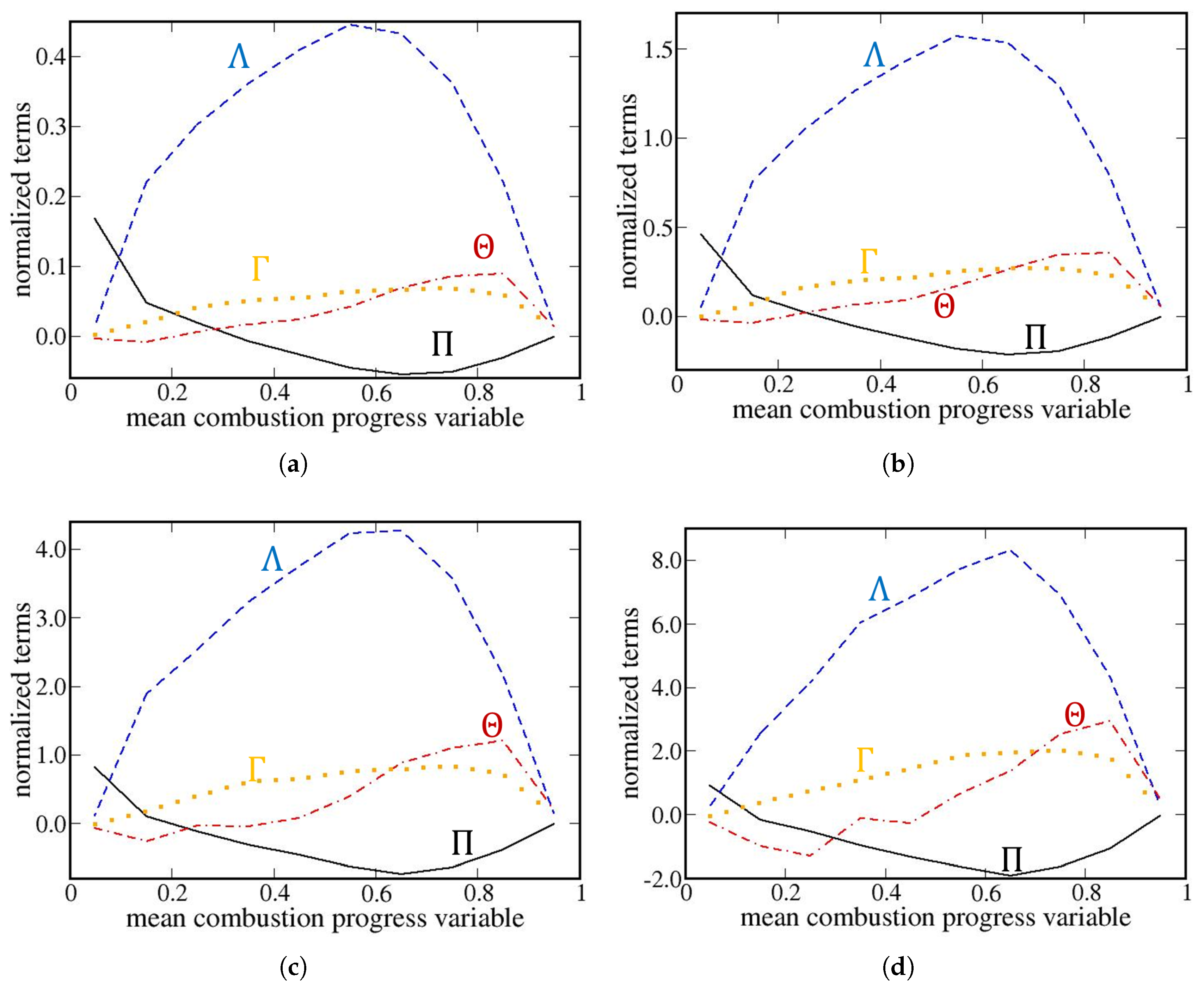
Figure 1 shows axial (longitudinal, along the normal to mean flame brush) variations in normalized (using ${\rho }_u{S}_L^3/{\delta }_L$, where $S_L$ and ${\delta }_L$ are laminar flame speed and thickness, respectively; ${\rho }_u$ is unburned gas density) time- and transverse-averaged (mean) values $\overline{\langle ·\rangle }$ of $\Pi$ (black solid lines), $\Lambda$ (blue dashed lines), $\Theta$ (red dotted-dashed lines), and $\Gamma$ (orange dotted lines). As stated in Section 2.3, x-dependencies are transformed to $\overline{\langle c\rangle }\left(x\right)$-dependencies here.

The following results shown in Figure 1 are worth noting. First, trends do not depend on the filter width.

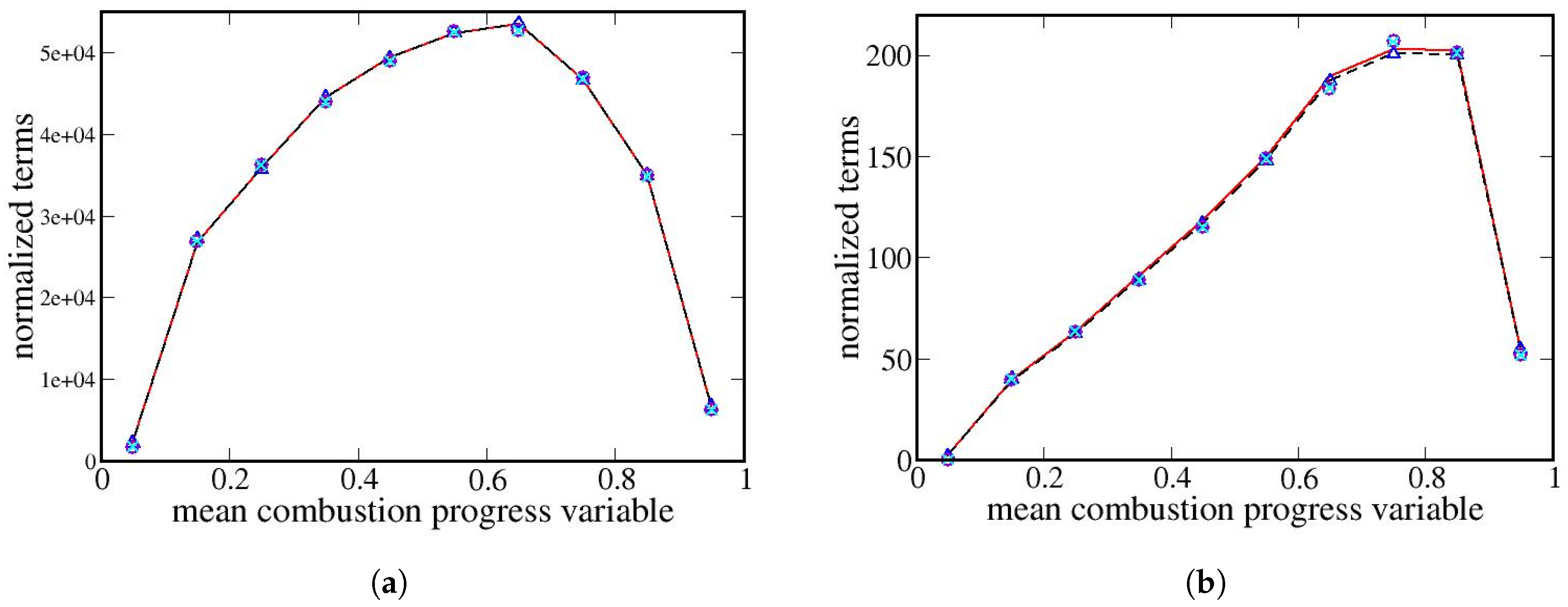
Second, the magnitudes of the mean terms $\overline{\langle \Pi \rangle }$, $\overline{\langle \Lambda \rangle }$, $\overline{\langle \Theta \rangle }$, and $\overline{\langle \Gamma \rangle }$ are decreased with decreasing the filter width $\Delta$. This trend is associated with the fact that magnitudes of $\widetilde{u_i{u}_j}-{\tilde{u}}_i{\tilde{u}}_j$, $\widetilde{u_i}-\overline{u_i}$, $\overline{p\nabla ·\mathit{u}}-\overline{p}\nabla ·\overline{\mathit{u}}$, and $\overline{\mathit{u}·\nabla p}-\overline{\mathit{u}}·\nabla \overline{p}$ tend to zero as $\Delta \to 0$. On the contrary, magnitudes of the mean subterms $\overline{p\nabla ·\mathit{u}}$, $\overline{p}\nabla ·\overline{\mathit{u}}$, $\overline{\mathit{u}·\nabla p}$, and $\overline{\mathit{u}}·\nabla \overline{p}$, depend weakly on $\Delta$, see Figure 2.

It is worth noting that these subterm magnitudes are much larger than magnitudes of the terms $\overline{\langle \Theta \rangle }$ and $\overline{\langle \Gamma \rangle }$, with this trend being greatly pronounced for the pressure–dilatation terms. The point is that contrary to low-Mach-number flows without heat release, where both local and mean dilatations are very small, magnitudes of the terms $\overline{p\nabla ·\mathit{u}}$ and $\overline{p}\nabla ·\overline{\mathit{u}}$ can be much larger than magnitudes of other terms in Equation (25) in flames, where significant (i.e., comparable with other velocity derivatives even after averaging) dilatation $\nabla ·\mathit{u}$ is multiplied with a very large pressure $p=O{\left(10\right)}^5$ N/m². Comparison of scales of ordinate axes in Figure 1 and Figure 2a does show that the two mean pressure–dilatation subterms are much larger than $\overline{\langle \Pi \rangle }$, $\overline{\langle \Lambda \rangle }$, $\overline{\langle \Gamma \rangle }$, or $\overline{\langle \Theta \rangle }$ evaluated using the same $\Delta$. Moreover, sensitivity of the pressure–dilatation subterms to filter width is very weak, see Figure 2a and note that results obtained using other filters are not reported, because these results are indistinguishable with the naked eye from the plotted results.

Third, magnitudes of $\overline{\langle \Pi \rangle }$ and $\overline{\langle \Gamma \rangle }$ or $\overline{\langle \Theta \rangle }$ are comparable, whereas their signs are often opposite. Specifically, $\overline{\langle \Pi \rangle }$ is positive at $\overline{\langle c\rangle }<0.3$, thus, indicating direct cascade in this leading zone of the mean flame brush. However, due to the influence of combustion-induced thermal expansion $\overline{\langle \Pi \rangle }<0$ at larger $\overline{\langle c\rangle }$, thus, indicating backscatter. Such a backscatter was already reported in earlier DNS studies of premixed turbulent flames [39,40,43,44,45,47,48,49]. The subfilter-scale pressure–dilatation term $\overline{\langle \Theta \rangle }$ is positive at $\overline{\langle c\rangle }>0.4$ indicating transfer of energy to subfilter-scale motions, but may be negative at lower $\overline{\langle c\rangle }$, indicating energy transfer in the opposite direction. The term $\Gamma$ is always positive, showing an increase in subfilter-scale kinetic energy due to combustion-induced thermal expansion. Indeed, since combustion-induced decrease in the local pressure within local flames results in increasing the local flow velocity in the normal direction to the flame surface, combustion-induced thermal expansion is expected to yield negative perturbations in the locally normal pressure gradient and positive perturbations in the locally normal flow velocity. Accordingly, correlation between $\nabla p$ and $\mathit{u}$ should be negative in the flame (if thermal expansion effects are sufficiently strong), resulting in $\Gamma >0$.

Fourth, $\overline{\langle \Lambda \rangle }$ is always positive, with its magnitude being significantly higher than magnitudes of $\overline{\langle \Pi \rangle }$ or $\overline{\langle \Gamma \rangle }$. Accordingly, $\overline{\langle \Pi \rangle }+\overline{\langle \Lambda \rangle }$ is positive, i.e., these two components of sfs transfer, considered jointly, yield direct cascade. Importance of $\Lambda$ was earlier observed in variable density, inert, low Mach number flows. Specifically, Lees and Aluie [28] reported positive $\Pi$ and negative $\Lambda$ in forced homogeneous compressible turbulence; Zhao et al. [34] documented positive $\Pi$ and positive $\Lambda$ in Rayleigh-Taylor turbulence; Zhou et al. [35] found transition from backscatter ($\Pi <0$) to downward transfer ($\Pi >0$) during evolution of Richtmyer-Meshkov turbulence, whereas $\Lambda$ was negative during the entire evolution stage with the exception of a short time interval during the transition phase.

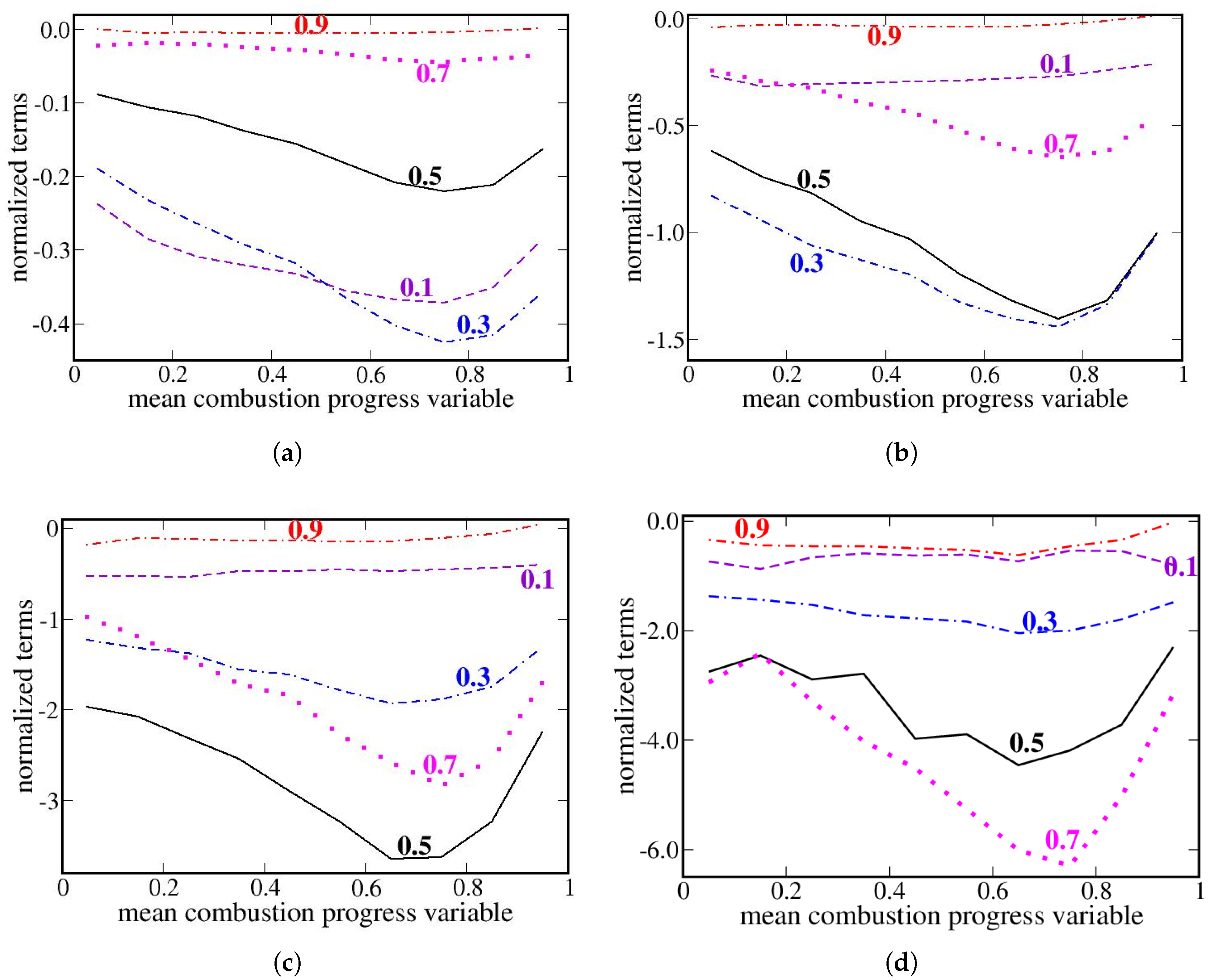
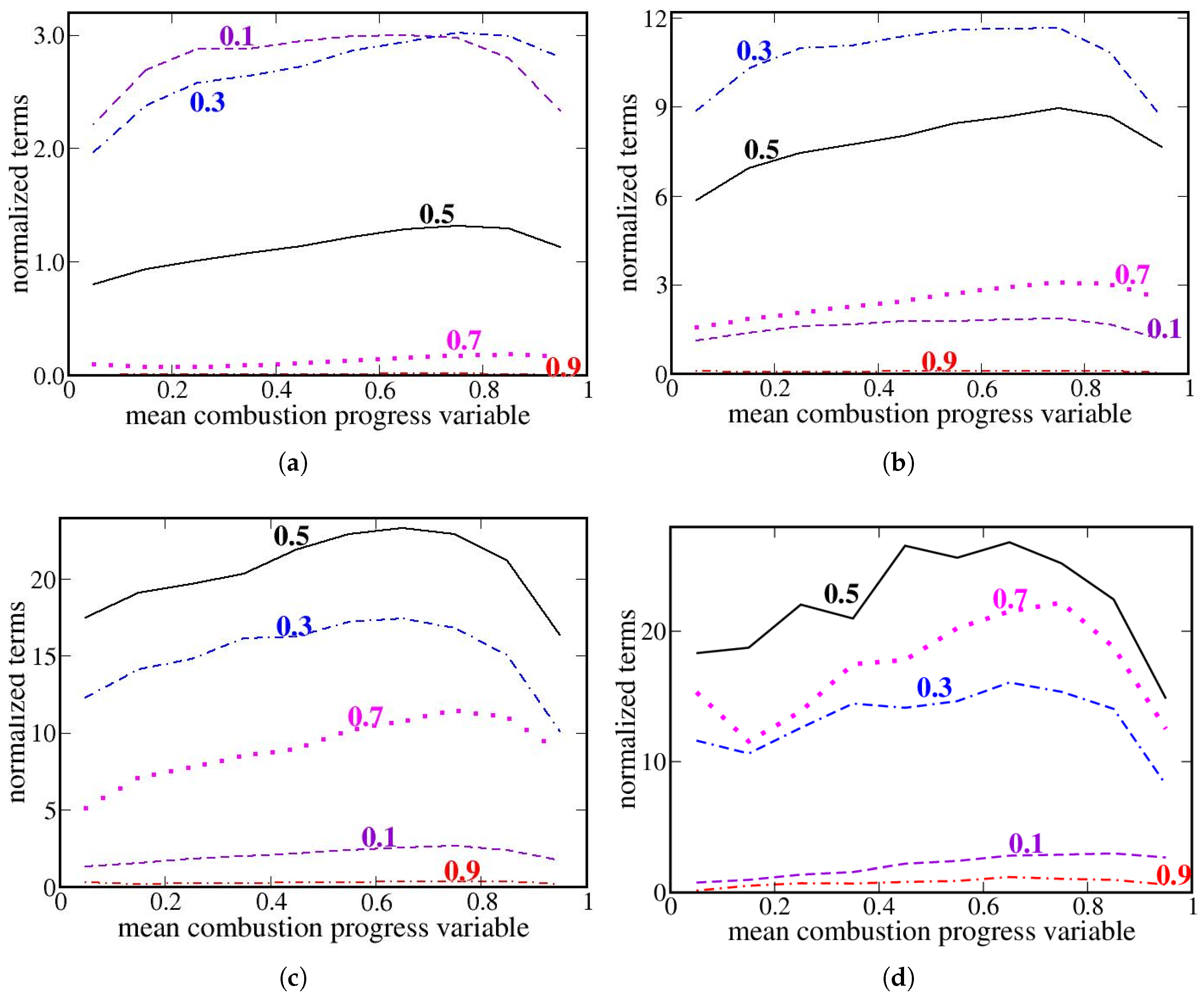
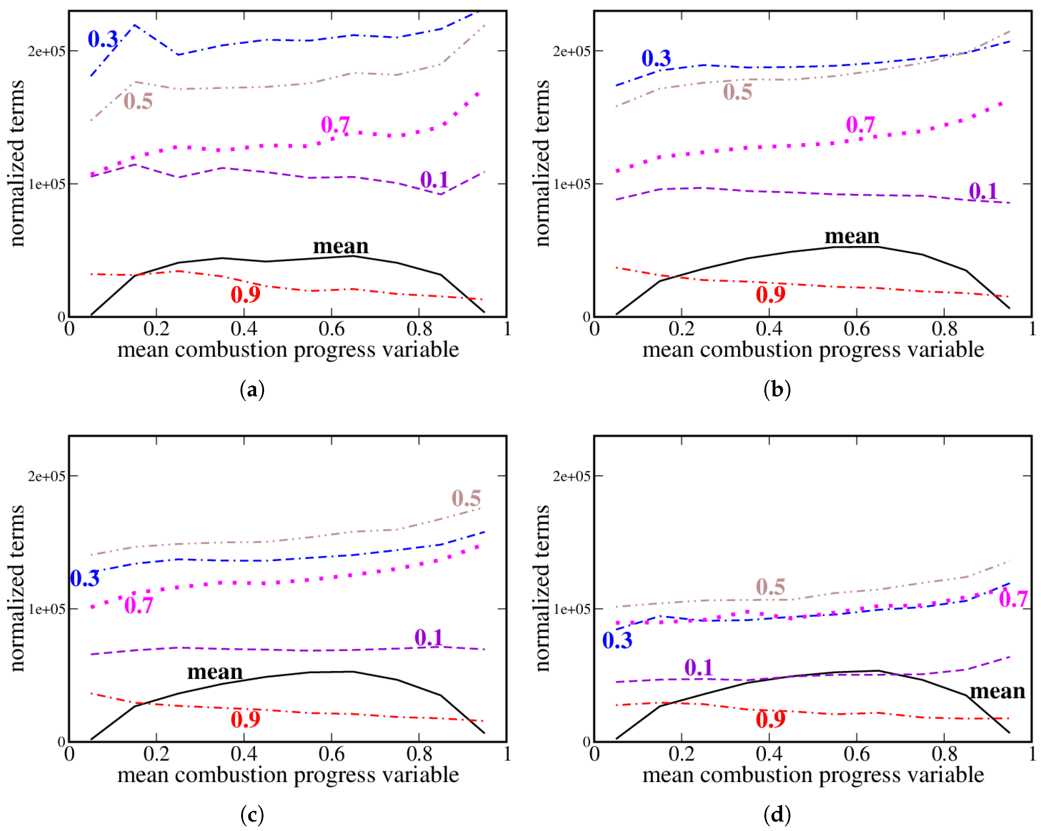
Figure 3 and Figure 4 show axial (longitudinal) variations in conditional terms $\langle T|\overline{c}=\xi ;\overline{\langle c\rangle }\rangle$, where $T=\Pi$ and $\Lambda$, respectively. Variations in the conditional terms $\langle T|\overline{c}=\xi ;\overline{\langle c\rangle }\rangle$, where $T=\Theta$ or $\Gamma$, are not reported here, because they were explored in our recent paper [58]. The following trends shown in these figures are worth noting.

First, the variations are large. Moreover, comparison of ordinate axes of Figure 1a–d with ordinate axes of Figure 3a–d and Figure 4a–d shows that magnitudes of certain conditional terms $\langle T|\overline{c}=\xi ;\overline{\langle c\rangle }\rangle$ are significantly larger than magnitudes of the counterpart mean terms $\overline{\langle T\rangle }$. For instance, for all adopted filters, magnitudes of the conditional $\Pi$-terms $\langle \Pi |0.45<\xi <0.55;\overline{\langle c\rangle }\rangle$, i.e., $\langle \Pi |\overline{c}=0.5;\overline{\langle c\rangle }\rangle$, see curves plotted in black solid lines in Figure 3, are significantly higher than magnitudes of $\overline{\langle \Pi \rangle }$, see curves plotted in black solid lines in Figure 1. In a similar way, for all adopted filters, magnitudes of the conditional $\Lambda$-terms $\langle \Lambda |0.25<\xi <0.35;\overline{\langle c\rangle }\rangle$ or $\langle \Lambda |0.45<\xi <0.55;\overline{\langle c\rangle }\rangle$, see curves plotted in blue dotted-double-dashed and black solid lines, respectively, in Figure 4, are significantly higher than magnitudes of $\overline{\langle \Lambda \rangle }$, see curves plotted in blue dashed lines in Figure 1.

The emphasized differences in the magnitudes of the mean and conditional terms are associated with the fact that magnitudes of velocity gradient, pressure gradient, and $|\overline{\mathit{u}}-\tilde{\mathit{u}}|$ are significantly increased within instantaneous local flames (called flamelets for brevity in the following) due to combustion-induced thermal expansion. For instance, dilatation is localized to thin zones in the studied flame [90]. When averaging is performed over a transverse plane, probability of finding such zones is low and the mean term is small. When averaging is performed over volumes characterized by $\overline{c}(\mathit{x},t)=0.1$, 0.3, 0.5 or 0.7, probability of finding such zones is significant. Therefore, magnitudes of the conditional terms $\langle T|\overline{c}=\xi ;\overline{\langle c\rangle }\rangle$ are large when compared to magnitudes of the mean terms $\overline{\langle T\rangle }$.

Second, magnitudes of conditional terms $\langle T|\overline{c}=\xi ;\overline{\langle c\rangle }\rangle$ obtained at $\xi =0.9$, see curves plotted in red dotted-dashed lines in Figure 3 and Figure 4, are much smaller than magnitudes of the same terms conditioned to a lower $\xi$. This difference is observed for all studied filter widths. On the contrary, variations in $\langle T|\overline{c}=\xi ;\overline{\langle c\rangle }\rangle$ with $\xi$ at smaller $\xi \le 0.7$ depend on the filter width. For instance, the term $\langle \Pi |\overline{c}=\xi ;\overline{\langle c\rangle }\rangle$ has the highest magnitude (i) at $\xi =0.3$ if $\Delta =0.22{\delta }_L$ or $\Delta =0.44{\delta }_L$, see curves plotted in blue dotted-double-dashed lines in Figure 3a,b; (ii) at $\xi =0.5$ if $\Delta =0.88{\delta }_L$, see curve plotted in black solid line in Figure 3c; and (iii) at $\xi =0.7$ if $\Delta =1.65{\delta }_L$, see curve plotted in magenta dotted line in Figure 3d. The term $\langle \Lambda |\overline{c}=\xi ;\overline{\langle c\rangle }\rangle$ has the highest magnitude (i) at $\xi =0.3$ if $\Delta =0.22{\delta }_L$ or $\Delta =0.44{\delta }_L$, see curves plotted in blue dotted-double-dashed lines in Figure 3a,b; but (ii) at $\xi =0.5$ if $\Delta =0.88{\delta }_L$ or $\Delta =1.65{\delta }_L$, see curves plotted in black solid lines in Figure 3c,d.

The observed influence of filter width on relations between magnitudes of the terms $\langle T|\overline{c}=\xi ;\overline{\langle c\rangle }\rangle$ conditioned to different $\xi$ is associated with $\Delta$-dependence of contributions from flamelets to these terms. For instance, the term $\Pi$ is expected to be positive upstream of flamelets and negative within the flamelets. Results plotted in Figure 1 are in line with this expectation, as $\overline{\langle \Pi \rangle }>0$ at small $\overline{\langle c\rangle }$, where the probability of finding flamelets is low, and $\overline{\langle \Pi \rangle }<0$ at larger $\overline{\langle c\rangle }$, where the probability of finding flamelets is substantial. These results also indicate that contribution to $\Pi$ from flamelets dominates contribution to $\Pi$ from reactants and combustion products in the largest part of the mean flame brush with the exception of small $\overline{\langle c\rangle }$. Accordingly, if $\Delta$ is small, the DNS data are filtered out over volumes where the local $c(\mathit{x},t)$ is sufficiently close to the filtered $\overline{c}(\mathit{x},t)$. Therefore, magnitude of the negative $\langle \Pi |\overline{c}=\xi ;\overline{\langle c\rangle }\rangle$ is expected to peak at $\xi$ that is close to the local value $c^{*}$ of the combustion progress variable associated with the highest velocity gradients within flamelets. Since the studied flame statistically retains the local structure of the unperturbed laminar premixed flame [55,56], the value of $c^{*}$ may be estimated using results of the simulations of that laminar flame. For the studied mixture, $c^{*}=0.36$. Consequently, $\langle \Pi |\overline{c}=\xi ;\overline{\langle c\rangle }\rangle$ has the highest magnitude at $\xi =0.3$ if $\Delta$ is small, see Figure 3a. If the filter width is increased and $\xi =0.3$ is retained, volumes characterized by small local $c(\mathit{x},t)$ (and associated with the positive $\Pi$) contribute more to $\langle \Pi |\overline{c}=\xi ;\overline{\langle c\rangle }\rangle$ and mitigate an increase in the term magnitude by $\Delta$. Indeed, dependence of $\langle \Pi |\overline{c}=\xi ;\overline{\langle c\rangle }\rangle$ on $\Delta$ is weakly pronounced in Figure 3 if $\xi =0.3$, cf. curves plotted in violet dashed lines in different subfigures. On the contrary, if the filter width is increased and $\xi =0.5$ or $0.7$, volumes characterized by $c(\mathit{x},t)\approx c^{*}=0.36$ contribute more to $\langle \Pi |\overline{c}=\xi ;\overline{\langle c\rangle }\rangle$, thus, increasing its magnitude, cf. curves plotted in black solid or magenta dotted lines in Figure 3a–d. A similar explanation, i.e., the $\Delta$-dependence of contributions from flamelets to $\langle T|\overline{c}=\xi ;\overline{\langle c\rangle }\rangle$, appears to hold for the term $T=\Lambda$.

Third, if the small values of $\langle \Pi |\overline{c}=\xi ;\overline{\langle c\rangle }\rangle$ at $\xi =0.9$ are disregarded, i.e., if $0.05\le \xi \le 0.75$, the conditional terms $\langle \Pi |\overline{c}=\xi ;\overline{\langle c\rangle }\rangle$ have the same sign (negative) for all filters, see Figure 3a–d. The terms $\langle \Lambda |\overline{c}=\xi ;\overline{\langle c\rangle }\rangle$ also have the same sign (but positive) for all filters if $0.05\le \xi \le 0.75$, see Figure 4a–d.

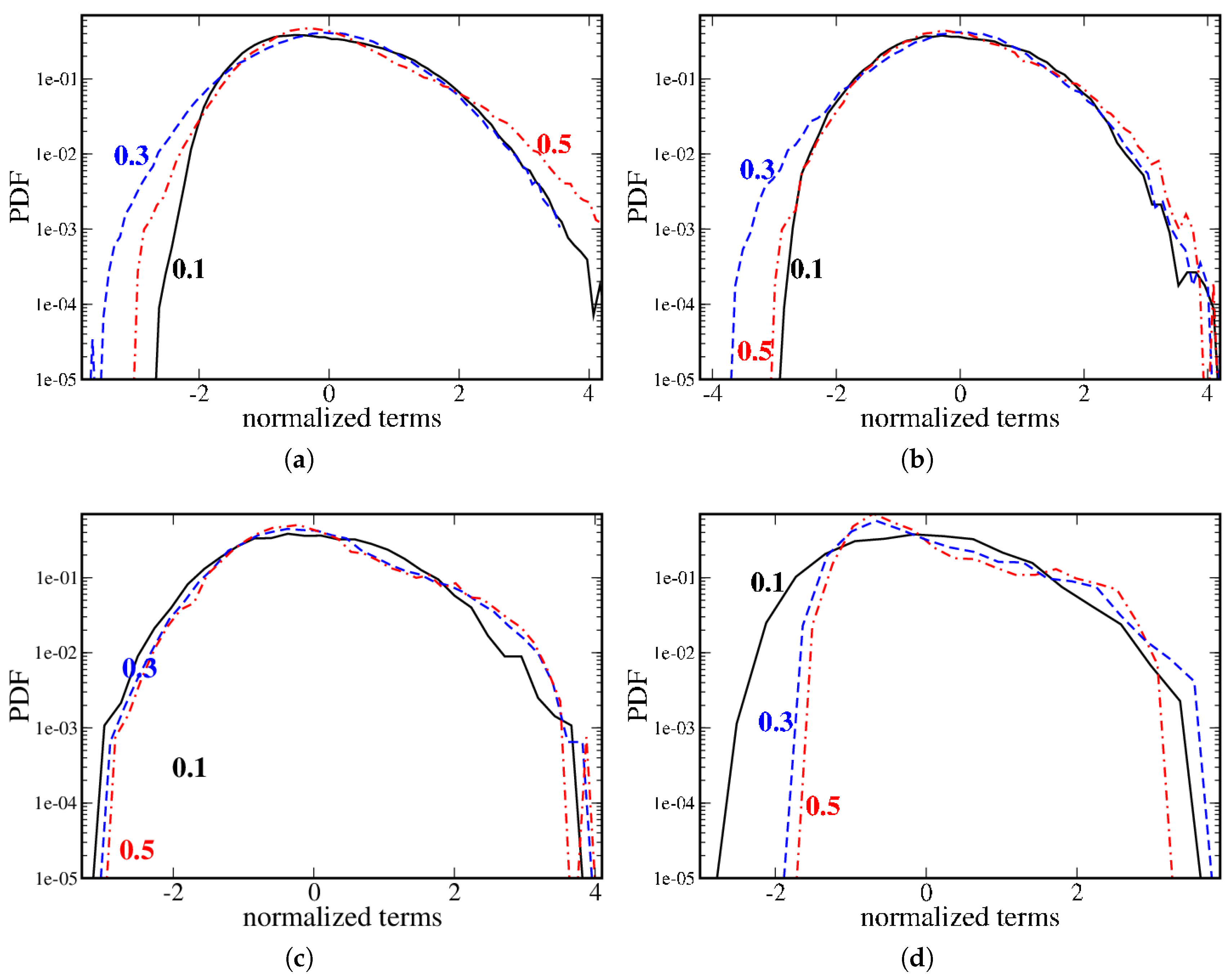
Curves plotted in color broken lines in Figure 5 show variations in the conditioned values $\langle \overline{p\nabla ·\mathit{u}}|\overline{c}=\xi ;\overline{\langle c\rangle }\rangle$ of the pressure–dilatation subterm $\overline{p\nabla ·\mathit{u}}$ with the sampling variable $\xi$, which is associated with the filtered combustion progress variable $\overline{c}(\mathit{x},t)$. Conditioned values of the second pressure–dilatation subterm $\overline{p}\nabla ·\overline{\mathit{u}}$ are not reported, because they are indistinguishable with the naked eye from the plotted results. While the conditional pressure–dilatation subterms depend weakly on filter width, some decrease in $\langle \overline{p\nabla ·\mathit{u}}|\overline{c}=\xi ;\overline{\langle c\rangle }\rangle$ with $\Delta$ is observed, because volumes characterized by a low dilatation $\nabla ·\mathit{u}$ contribute more to $\langle \overline{p\nabla ·\mathit{u}}|\overline{c}=0.3;\overline{\langle c\rangle }\rangle$ or $\langle \overline{p\nabla ·\mathit{u}}|\overline{c}=0.5;\overline{\langle c\rangle }\rangle$ if the filter width is increased. This trend is more pronounced at $\xi =0.3$, because probabilities of finding small local $c(\mathit{x},t)$ and, hence, small local dilatation $\nabla ·\mathit{u}$ are expected to be higher in filter volumes characterized by $\overline{c}(\mathit{x},t)=0.3$ when compared to volumes characterized by $\overline{c}(\mathit{x},t)=0.5$, provided that $\Delta$ is sufficiently large. Accordingly, the conditional pressure–dilatation subterms have the highest magnitude if $\xi =0.3$ and $\Delta \le 0.44{\delta }_L$ or if $\xi =0.5$ and $\Delta \ge 0.88{\delta }_L$, see curves plotted in blue dotted-double-dashed lines in Figure 5a,b or curves plotted in brown double-dotted-dashed lines in Figure 5c,d. The mean term $\overline{\langle \overline{p\nabla ·\mathit{u}}\rangle }$ (i) depends weakly on filter width, cf. curves plotted in black solid lines in Figure 5a–d, and (ii) is significantly smaller than the terms conditioned to $0.3\le \xi \le 0.7$. The latter trend is attributed to a higher (lower) probability of finding significant local dilatation when evaluating the conditional (mean) terms.

3.2. Probability Density Functions

Since intermittency in turbulent flows is well known to significantly change the shapes of PDFs of relevant quantities [2,3,52], let us explore intermittency of the analyzed random filtered fields by investigating their standardized conditional PDFs computed using Equations (34)–(38) and averaged over the length of the computational domain. Such PDFs do not depend on x and are designated as follows: ${\widehat{P}}_{q|c}\left(s\right|\xi )=\sigma {\widehat{P}}_{q|c}\left(\psi \right|\xi )$.

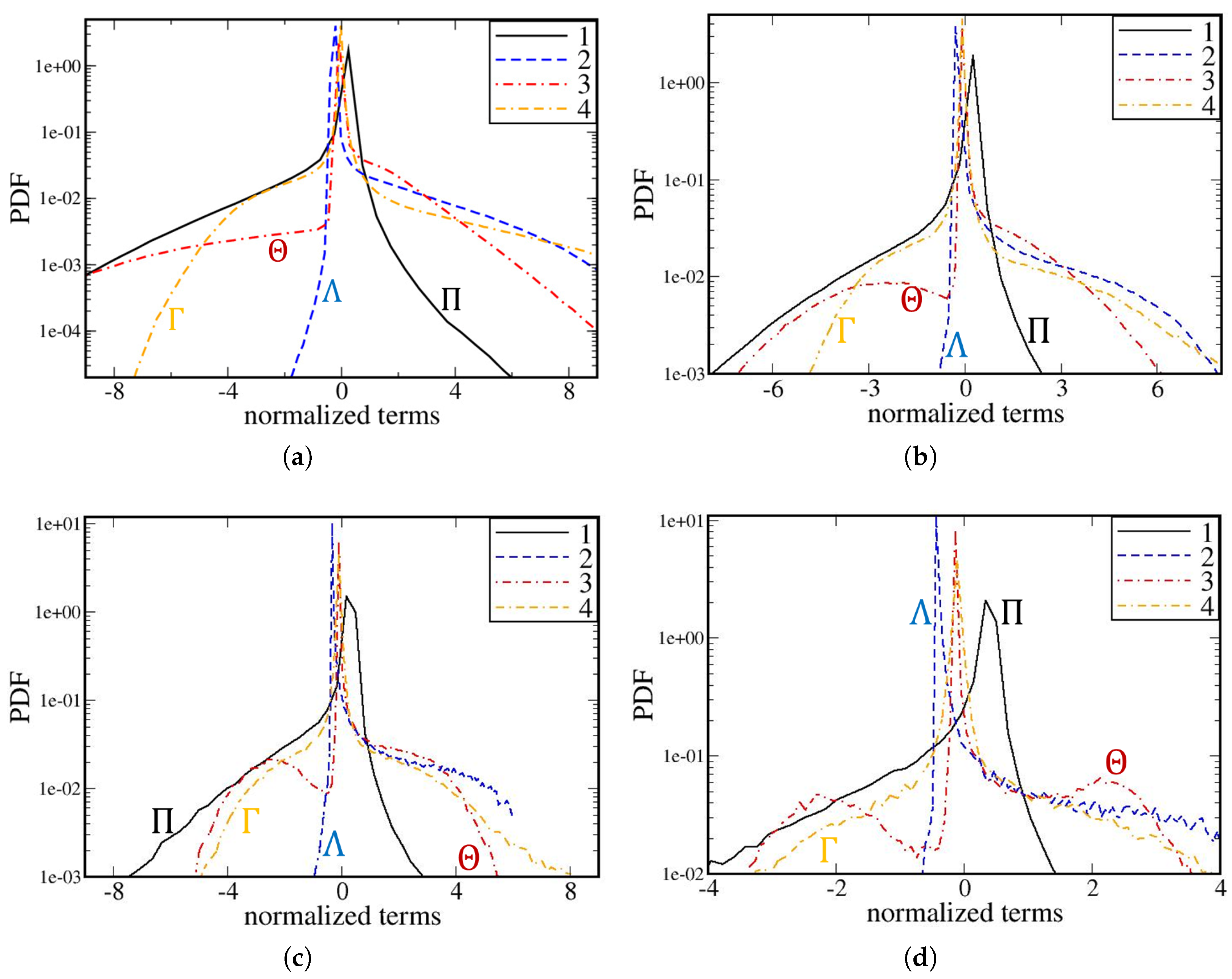
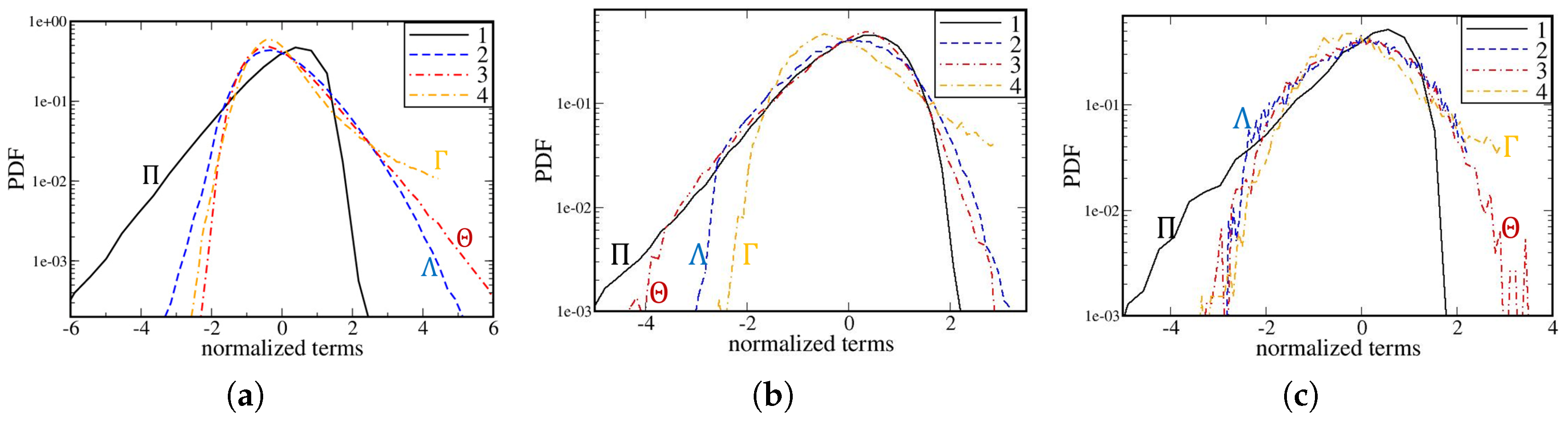
Figure 6 and Figure 7 report the averaged standardized conditional PDFs ${\widehat{P}}_{q|c}\left(s\right|0.05\le \xi \le 0.95)$ and ${\widehat{P}}_{q|c}\left(s\right||\overline{c}(\mathit{x},\mathit{t})-\xi |\le 0.05)$, respectively, for the four terms associated with energy transfer to subfilter-scale motions, i.e., $\Pi$ (black solid lines), $\Lambda$ (blue dotted lines), $\Theta$ (red dotted-dashed lines), and $\Gamma$ (orange dotted lines).

The standardized conditional PDFs ${\widehat{P}}_{q|c}\left(s\right|0.05\le \xi \le 0.95)$ are very different from the Gaussian distribution. For all four terms, the PDFs are characterized by a very large kurtosis, which is decreased with increasing $\Delta /{\delta }_L$, see

Table 1. Skewness ${\mu }_3/{\sigma }^3$ and kurtosis ${\mu }_4/{\sigma }^4$ of PDFs for various normalized filtered terms.

Terms	$\mathbf{\Delta }=0.22{\mathit{\delta }}_{\mathit{L}}$		$\Delta =0.44{\mathit{\delta }}_{\mathit{L}}$		$\Delta =0.88{\mathit{\delta }}_{\mathit{L}}$		$\Delta =1.65{\mathit{\delta }}_{\mathit{L}}$
	${\mathit{\mu }}_{\mathbf{3}}/{\mathbf{\sigma }}^{\mathbf{3}}$	${\mathit{\mu }}_{\mathbf{4}}/{\mathbf{\sigma }}^{\mathbf{4}}$	${\mathit{\mu }}_{\mathbf{3}}/{\mathbf{\sigma }}^{\mathbf{3}}$	${\mathit{\mu }}_{\mathbf{4}}/{\mathbf{\sigma }}^{\mathbf{4}}$	${\mathit{\mu }}_{\mathbf{3}}/{\mathbf{\sigma }}^{\mathbf{3}}$	${\mathit{\mu }}_{\mathbf{4}}/{\mathbf{\sigma }}^{\mathbf{4}}$	${\mathit{\mu }}_{\mathbf{3}}/{\mathbf{\sigma }}^{\mathbf{3}}$	${\mathit{\mu }}_{\mathbf{4}}/{\mathbf{\sigma }}^{\mathbf{4}}$
$0.05<\overline{c}(\mathit{x},t)<0.95$
$\Pi$	−5.57	44.7	−4.58	31.1	−3.59	21.6	−2.49	11.9
$\Lambda$	5.50	38.0	4.62	26.2	3.69	16.6	2.75	9.84
$\Theta$	−2.52	50.9	−0.59	21.8	0.51	11.5	0.43	6.75
$\Gamma$	2.70	29.0	2.66	23.0	2.10	18.5	1.19	11.3
$\overline{p}\nabla ·\overline{\mathit{u}}$	3.03	12.3	2.69	9.93	2.18	6.86	1.60	4.39
$0.05<\overline{c}(\mathit{x},t)<0.15$
$\Pi$	−2.47	22.9	−2.53	26.3	−2.24	28.2	−3.37	28.6
$\Lambda$	1.20	4.32	0.89	3.68	0.86	3.86	0.80	3.78
$\Theta$	−0.85	3.67	−0.51	3.02	−0.30	2.88	−0.09	2.93
$\Gamma$	−0.29	3.08	−0.13	3.45	−0.19	3.28	−0.24	3.03
$\overline{p}\nabla ·\overline{\mathit{u}}$	0.40	2.71	0.19	2.62	0.19	2.73	0.28	2.73
$0.25<\overline{c}(\mathit{x},t)<0.35$
$\Pi$	−0.90	4.25	−1.01	5.08	−1.30	5.37	−1.13	4.74
$\Lambda$	0.36	2.84	−0.17	2.78	−0.19	2.54	0.08	2.48
$\Theta$	−0.59	6.23	−0.70	3.83	−0.01	2.78	−0.006	2.56
$\Gamma$	0.84	3.42	0.64	3.07	0.54	3.30	−0.09	2.86
$\overline{p}\nabla ·\overline{\mathit{u}}$	0.11	2.97	0.004	3.10	0.58	3.30	0.86	3.17
$0.45<\overline{c}(\mathit{x},t)<0.55$
$\Pi$	−1.03	4.78	−0.98	4.46	−0.92	3.89	−1.04	3.96
$\Lambda$	0.48	3.58	0.34	2.99	−0.68	2.87	−0.60	2.59
$\Theta$	1.05	4.69	0.54	3.38	0.05	3.28	0.25	3.11
$\Gamma$	1.64	3.33	1.63	5.94	1.23	4.24	0.70	2.96
$\overline{p}\nabla ·\overline{\mathit{u}}$	0.70	3.72	0.42	3.06	0.72	3.46	1.04	3.18

. The PDFs of $\Pi$, see curves plotted in black solid lines in Figure 6, are characterized by a highly negative skewness, whose magnitude is also decreased with increasing $\Delta /{\delta }_L$ (see Table 1), and have long upward tails, which look like a stretched exponential tail. These standardized conditional PDFs of $\Pi$ appear to differ substantially from standardized conditional PDFs of $\Pi$ in incompressible or high-speed compressible turbulence. For instance, PDFs for $\Pi$ in Rayleigh–Taylor turbulence manifest a strong skewness toward the positive sides [34], while information about such PDFs in statistically inhomogeneous flows is still rare.

The PDF of $\Lambda$ is characterized by a highly positive skewness, contrary to homogeneous compressible turbulence [26], but in line with recent results obtained from Rayleigh–Taylor turbulence [34]. The $\Lambda$-skewness is also decreased with increasing $\Delta /{\delta }_L$; see Table 1. The tails of the standardized conditional PDFs of $\Lambda$ appear to be a combination of exponential and downward branches, see curves plotted in red dotted-dashed lines.

The PDFs of $\Gamma$, see curves plotted in orange dotted lines in Figure 6, look more symmetrical when compared to the standardized conditional PDFs of $\Pi$ or $\Lambda$. Nevertheless, the standardized conditional PDFs of $\Gamma$ are still characterized by a positive skewness, which is also decreased with increasing $\Delta /{\delta }_L$; see Table 1. The present authors are not aware of a publication where a PDF of $\Gamma$ is reported for a turbulent flow.

The standardized conditional PDFs of $\Theta$ are more sensitive to the filter width, thus further demonstrating issues (small difference between two large terms) with a priori studies of the field $\Theta$ in premixed turbulent flames. The appearance of the left peaks in curves plotted in red dotted-dashed lines in Figure 6b–d could be attributed to such numerical issues, while locally negative dilatation $\nabla ·\mathit{u}$ was documented in the studied flame [90].

All in all, the four standardized conditional PDFs ${\widehat{P}}_{q|c}\left(s\right|0.05\le \xi \le 0.95)$ shown in Figure 6, as well as their moments reported in Table 1, indicate strong intermittency of the studied filtered fields. Moreover, these PDFs demonstrate a distinct/particular place of low Mach number turbulent premixed flame when compared to other turbulent flows. The reported PDFs imply that the intermittency of inter-scale energy transfer and energy exchange between internal and kinetic energies depends strongly on methods and scales of energy injection.

The intermittency is less pronounced for PDFs conditioned to a small interval of $\overline{c}(\mathit{x},t)$. For instance, such PDFs plotted in Figure 7 have shorter tails when compared to the counterpart PDFs presented in Figure 6. Moreover, the conditional PDFs are characterized by sufficiently small skewness and kurtosis, see Table 1, with the exception of the PDF of $\Pi$.

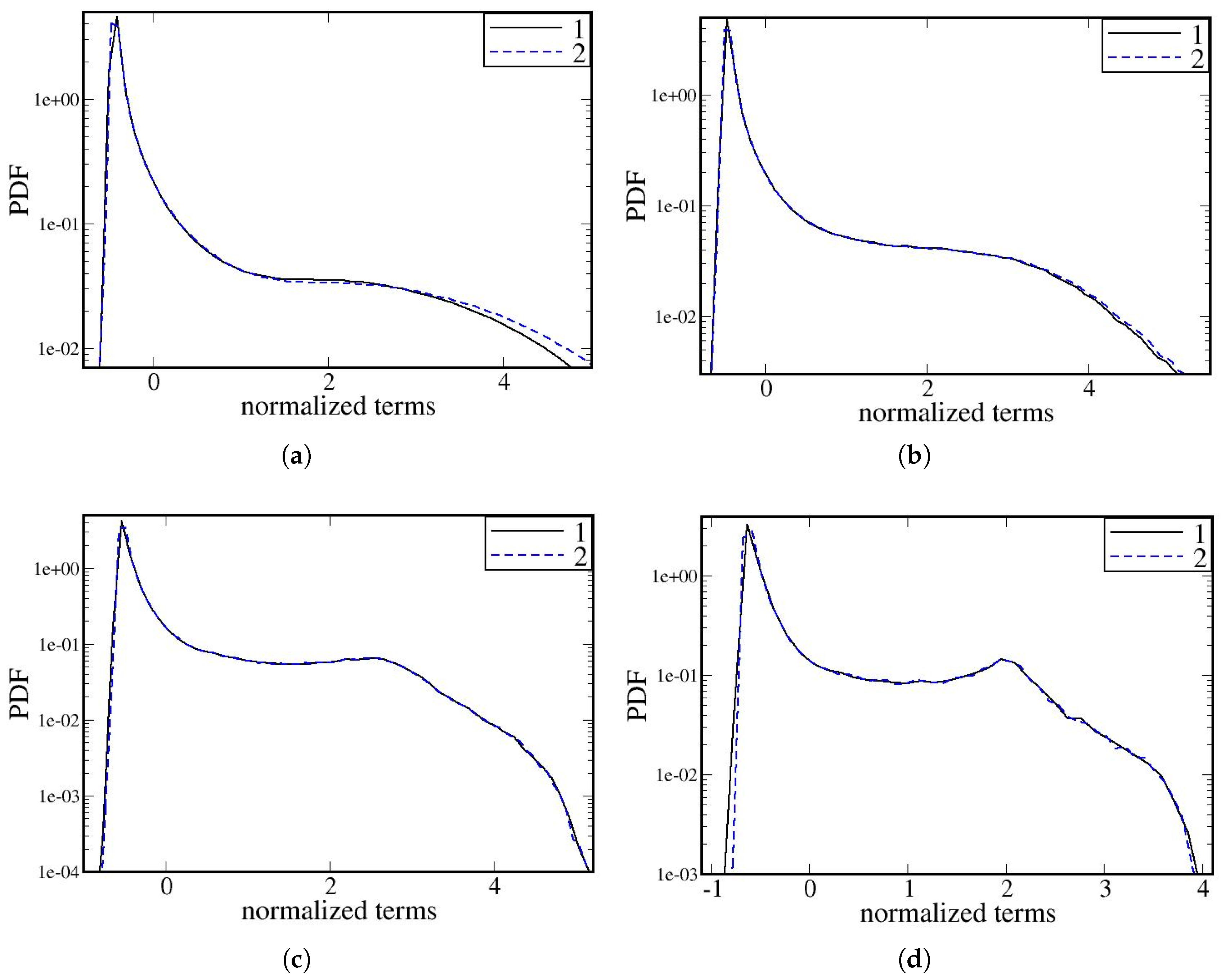
Figure 8 and Figure 9 report PDFs of terms that are often associated with the transfer of resolved internal energy to resolved and filtered motions, i.e., the resolved pressure–dilatation term $\overline{p}\nabla ·\overline{\mathit{u}}$ and the filtered pressure–dilatation term $\overline{p\nabla ·\mathit{u}}$. It is worth noting that at a low Mach number typical for a free turbulent premixed flame, pressure variations within the flame brush are small, i.e., $\left|p\right(\mathit{x},t)-P|\ll P$, where P is the thermodynamic pressure [91,92]. Therefore, $\overline{p}\nabla ·\overline{\mathit{u}}\approx \overline{p\nabla ·\mathit{u}}\approx P\nabla ·\overline{\mathit{u}}$. The analyzed DNS data do show that $\overline{p}\nabla ·\overline{\mathit{u}}$ and $\overline{p\nabla ·\mathit{u}}$ are indistinguishable to the naked eye, as expected. For this reason, the PDFs of the former term are only presented in Figure 8 and Figure 9. Moreover, comparison of curves plotted in black solid and blue dashed lines in Figure 8 shows that the standardized conditional PDFs ${\widehat{P}}_{q|c}\left(s\right|0.05\le \xi \le 0.95)$ defined by Equations (34)–(38) are very close for the normalized filtered term $\overline{p}\nabla ·\overline{\mathit{u}}$ and the normalized filtered dilatation $\nabla ·\overline{\mathit{u}}$ independently of $\Delta /{\delta }_L$. This result further confirms that $\overline{p}\nabla ·\overline{\mathit{u}}\approx \overline{p\nabla ·\mathit{u}}$. Nevertheless, much smaller subfilter-scale pressure–dilatation term $\Theta$ does not vanish; see curves plotted in red dotted-dashed lines in Figure 1.

The standardized conditional PDFs ${\widehat{P}}_{q|c}\left(s\right|0.05\le \xi \le 0.95)$ of $q=\overline{p}\nabla ·\overline{\mathit{u}}$ and $q=\nabla ·\overline{\mathit{u}}$, reported in Figure 8, indicate that the two fields are highly intermittent. Indeed, these PDFs have heavy right tails and are positively skewed (see Table 1), contrary to incompressible or high-speed compressible turbulence. These features of the reported PDFs imply rare but intense energy flux from internal energy to fluid motion due to positive velocity divergence generated in zones that heat release and density variations are localized to. Reverse energy flux from fluid motion to internal energy is less efficient. Small values of the PDFs along the heavy right tails indicate that the volume of the aforementioned zones is essentially smaller than the entire flame-brush volume. The skewness and kurtosis of the standardized conditional PDFs are both significant and are decreased with increasing $\Delta /{\delta }_L$, see Table 1.

The counterpart PDFs conditioned to the filtered combustion progress variable have significantly shorter right tails (see Figure 9), thus indicating that the intensity of energy exchange between internal and kinetic energies is weaker within the conditional framework. Moreover, the conditional PDFs are characterized by a lower skewness whose magnitude is always smaller than unity, see Table 1. Furthermore, the flatness of the standardized conditional PDF ${\widehat{P}}_{q|c}\left(s\right||\overline{c}(\mathit{x},t)-\xi |\le 0.05)$ for $\xi =0.1$, $\xi =0.3$, or $\xi =0.5$ is also smaller when compared to the flatness of the standardized conditional PDF ${\widehat{P}}_{q|c}\left(s\right|0.05<\xi <0.95)$ and is sufficiently close to a value of 3.0, associated with the Gaussian distribution. All in all, a comparison of Figure 8 and Figure 9, as well as data reported in Table 1, indicates that intermittency is much less pronounced for the conditional resolved pressure–dilatation term $\overline{p}\nabla ·\overline{\mathit{u}}$. This trend may be attributed to the fact that conditional quantities are obtained from volumes characterized by close filtered values $\overline{c}(\mathit{x},t)$. Since such statistics are homogeneous in combustion progress variable space, relevant statistics of the energy transport related fields are also uniform.

4. Concluding Remarks

Velocity, pressure, and combustion-progress-variable fields generated in earlier three-dimensional direct numerical simulations [53,54] of a statistically stationary, planar, one-dimensional, low-Mach-number lean hydrogen–air flame propagating in moderately intense, small-scale, spatially decaying turbulence were filtered out using top-hat filters of four different widths. The filtered fields were processed to compute key source/sink terms in the transport equations for total, resolved, and subfilter-scale kinetic energies, as well as total internal energy. A priori analysis of these filtered terms has shown the following trends.

First, independently of filter width and averaging method, i.e., either transverse averaging or conditional averaging, the terms $\Pi$ and $\Lambda$, associated with inertial transfer of kinetic energy between resolved and subfilter scales and baropycnal work, respectively, serve to cause backscatter and forward scatter, respectively, with the baropycnal work dominating the former term. The velocity–pressure–gradient term $\Gamma$ is positive, indicating an increase in subfilter-scale kinetic energy. Under the conditions of the present study, the magnitude of $\Gamma$ is smaller when compared to the term $\Lambda$. The pressure–dilatation term $\Theta$ changes its sign from negative at small $\overline{\langle c\rangle }$ to positive at larger $\overline{\langle c\rangle }$. Under conditions of the present study, the magnitude of $\Theta$ is smaller when compared to the term $\Lambda$.

Second, the analyzed filtered fields indicate significant intermittency of inter-scale energy transfer and of energy exchange between internal and kinetic energy in turbulent premixed flames. This conclusion is based on analyses of Probability Density Functions of (i) the two filtered inter-scale kinetic energy transfer terms, $\Pi$ and $\Lambda$, and (ii) the filtered velocity–pressure–gradient term $\Gamma$ or the filtered pressure–dilatation term $\Theta$, and (iii) two almost equal terms $\overline{p·\nabla \mathit{u}}$ and $\overline{p}\nabla ·\overline{\mathit{u}}$ relevant to energy exchange between internal and kinetic energies. These PDFs exhibit long tails, are highly skewed, and are characterized by a large kurtosis, thus implying the appearance of relatively rare but vigorous ejection (splash) events. Moreover, a comparison of these standardized conditional PDFs with published conditional PDFs in incompressible or high-speed compressible turbulent flows indicates that intermittency of inter-scale energy transfer and energy exchange between internal and kinetic energies depends strongly on methods and scales of energy injection. Thus, premixed turbulent combustion is a canonical example of variable-density turbulent flows with distinctive characteristics that the differ substantially from characteristics of other types of turbulence. Therefore, studies of turbulent premixed flames constitute an important addition to the fundamental research into turbulence.

When analyzing filtered quantities conditioned to a narrow interval of filtered combustion progress variable, intermittency effects are substantially less prominent.

The reported results can be used for assessment of Subgrid Scale Models (SGS) models that were already developed to allow for backscatter of turbulent energy and scalar variance, but in non-reacting constant-density flows, e.g., see Ref. [93]. The present a priori study also emphasizes the importance of developing subfilter-scale models of baropycnal work and velocity–pressure–gradient work for LES research into premixed turbulent combustion. Such models should allow for both solenoidal and dilatational components of the velocity vector, as well as interactions between them. As an example, a recent gradient model of the baropycnal work validated in simulations of forced compressible turbulence in a periodic box [28,35] is worth considering. In this regard, a recent assessment of gradient models of the terms $\Pi$, $\Lambda$, $\Gamma$, and $\Theta$, performed by analyzing the present DNS data [53,54], yielded encouraging results [57,58].

References

1. Kolmogorov, A.N. The local structure of turbulence in incompressible viscous fluid for very large Reynolds number. Dokl. Akad. Nauk. SSSR 1941, 30, 299–303. [Google Scholar] [CrossRef]
2. Monin, A.S.; Yaglom, A.M. Statistical Fluid Mechanics: Mechanics of Turbulence; The MIT Press: Cambridge, MA, USA, 1975; Volume 2. [Google Scholar]
3. Frisch, U. Turbulence: The Legacy of A.N. Kolmogorov; Cambridge University Press: Cambridge, UK, 1995. [Google Scholar]
4. Richardson, L.F. Weather Prediction by Numerical Process; Cambridge University Press: Cambridge, UK, 2022. [Google Scholar]
5. Alexakis, A.; Biferale, L. Cascades and transitions in turbulent flows. Phys. Rep. 2018, 767–769, 1–101. [Google Scholar] [CrossRef]
6. Leslie, D.C.; Quarini, G.L. The application of turbulence theory to the formulation of subgrid modelling procedures. J. Fluid Mech. 1979, 91, 65–91. [Google Scholar] [CrossRef]
7. Piomelli, U.; Cabot, W.H.; Moin, P.; Lee, S. Subgrid-scale backscatter in turbulent and transitional flows. Phys. Fluids 1991, 3, 1766–1771. [Google Scholar] [CrossRef]
8. Domaradzki, A.; Liu, W.; Brachet, M.E. An analysis of subgrid-scale interactions in numerically simulated isotropic turbulence. Phys. Fluids A 1993, 5, 1747–1759. [Google Scholar] [CrossRef]
9. Cerutti, S.; Meneveau, C. Intermittency and relative scaling of subgrid-scale energy dissipation in isotropic turbulence. Phys. Fluids 1998, 10, 928–937. [Google Scholar] [CrossRef]
10. Borue, V.; Orszag, S.A. Local energy flux and subgrid-scale statistics in three-dimensional turbulence. J. Fluid Mech. 1988, 366, 1–31. [Google Scholar] [CrossRef]
11. Aoyama, T.; Ishihara, T.; Kaneda, Y.; Yokokawa, M.; Itakura, K.; Uno, A. Statistics of energy transfer in high-resolution direct numerical simulation of turbulence in a periodic box. J. Phys. Soc. Jpn. 2005, 74, 3202–3212. [Google Scholar] [CrossRef][Green Version]
12. Goto, S. A physical mechanism of the energy cascade in homogeneous isotropic turbulence. J. Fluid Mech. 2008, 605, 355–366. [Google Scholar] [CrossRef]
13. Ishihara, T.; Gotoh, T.; Kaneda, Y. Study of high-Reynolds number isotropic turbulence by direct numerical simulation. Annu. Rev. Fluid Mech. 2009, 41, 165–180. [Google Scholar] [CrossRef]
14. Yasuda, T.; Vassilicos, J.C. Spatio-temporal intermittency of the turbulent energy. J. Fluid Mech. 2018, 853, 235–252. [Google Scholar] [CrossRef]
15. Larssen, H.S.; Vassilicos, J.C. Spatio-temporal fluctuations of interscale and interspace energy transfer dynamics in homogeneous turbulence. J. Fluid Mech. 2023, 969, A14. [Google Scholar] [CrossRef]
16. Larssen, H.S.; Vassilicos, J.C. Turbulent energy transfers in physical and scale spaces at dissipative length scales. J. Fluid Mech. 2023, 976, A27. [Google Scholar] [CrossRef]
17. Qi, Y.; Meneveau, C.; Voth, G.A.; Ni, R. Folding dynamics and its intermittency in turbulence. Phys. Rev. Lett. 2023, 130, 154001. [Google Scholar] [CrossRef]
18. Yao, H.; Yeung, P.K.; Zaki, T.A.; Meneveau, C. Forward and inverse energy cascade and fluctuation relation in fluid turbulence adhere to Kolmogorov’s refined similarity hypothesis. Phys. Rev. Lett. 2024, 132, 164001. [Google Scholar] [CrossRef]
19. Yao, H.; Schnaubelt, M.; Szalay, A.S.; Zaki, T.A.; Meneveau, C. Comparing local energy cascade rates in isotropic turbulence using structure-function and filtering formulations. J. Fluid Mech. 2024, 980, A42. [Google Scholar] [CrossRef]
20. Jiménez, C.; Valiño, L.; Dopazo, C. A priori and a posteriori tests of subgrid scale models for scalar transport. Phys. Fluids 2001, 13, 2433–2436. [Google Scholar] [CrossRef]
21. Kobayashi, H. The subgrid-scale models based on coherent structures for rotating homogeneous turbulence and turbulent channel flow. Phys. Fluids. 2005, 17, 045104. [Google Scholar] [CrossRef]
22. Marstorp, L.; Brethouwer, G.; Johansson, A.V. A stochastic subgird model with application to turbulent flow and scalar mixing. Phys. Fluids 2007, 19, 035107. [Google Scholar] [CrossRef]
23. Aluie, H. Compressible turbulence: The cascade and its locality. Phys. Rev. Lett. 2011, 106, 174502. [Google Scholar] [CrossRef]
24. Aluie, H.; Li, S.; Li, H. Conservative cascade of kinetic energy in compressible turbulence. Astrophys. J. Lett. 2012, 751, L29. [Google Scholar] [CrossRef]
25. Aluie, H. Scale decomposition in compressible turbulence. Phys. D 2013, 247, 54–65. [Google Scholar] [CrossRef]
26. Wang, J.; Yang, Y.; Shi, Y.; Xiao, Z.; He, X.T.; Chen, S. Cascade of kinetic energy in three-dimensional compressible turbulence. Phys. Rev. Lett. 2013, 110, 214505. [Google Scholar] [CrossRef] [PubMed]
27. Wang, J.; Wan, M.; Chen, S.; Chen, S. Kinetic energy transfer in compressible isotropic turbulence. J. Fluid Mech. 2018, 841, 581–613. [Google Scholar] [CrossRef]
28. Lees, A.; Aluie, H. Baropycnal work: A mechanism for energy transfer across scales. Fluids 2019, 4, 92. [Google Scholar] [CrossRef]
29. Livescu, D. Turbulence with large thermal and compositional density variations. Annu. Rev. Fluid Mech. 2020, 52, 309–341. [Google Scholar] [CrossRef]
30. Teng, J.; Wang, J.; Li, H.; Chen, S. Spectra and scaling in chemically reacting compressible isotropic turbulence. Phys. Rev. Fluids 2020, 5, 084601. [Google Scholar] [CrossRef]
31. Wang, J.; Wan, M.; Chen, S.; Xie, C.; Zheng, Q.; Wang, L.-P.; Chen, S. Effect of flow topology on the kinetic energy flux in compressible isotropic turbulence. J. Fluid Mech. 2020, 883, A11. [Google Scholar] [CrossRef]
32. Teng, J.; Wang, J.; Li, H.; Chen, S. Kinetic energy transfer in compressible homogeneous anisotropic turbulence. Phys. Rev. Fluids 2021, 6, 064601. [Google Scholar] [CrossRef]
33. Wang, X.; Wang, J.; Li, H.; Chen, S. Interscale kinetic energy transfer in chemically reacting compressible isotropic turbulence. J. Fluid Mech. 2021, 912, A36. [Google Scholar] [CrossRef]
34. Zhao, D.; Betti, R.; Aluie, H. Scale interactions and anisotropy in Rayleigh-Taylor turbulence. J. Fluid Mech. 2022, 930, A29. [Google Scholar] [CrossRef]
35. Zhou, Z.; Ding, J.; Cheng, W. Mixing and inter-scale energy transfer in Richtmyer-Meshkov turbulence. J. Fluid Mech. 2024, 984, A56. [Google Scholar] [CrossRef]
36. Sabelnikov, V.A.; Yu, R.; Lipatnikov, A.N. Thin reaction zones in constant-density turbulent flows at low Damköhler numbers: Theory and simulations. Phys. Fluids 2019, 31, 055104. [Google Scholar] [CrossRef]
37. Driscoll, J.F.; Chen, J.H.; Skiba, A.W.; Carter, C.D.; Hawkes, E.R.; Wang, H. Premixed flames subjected to extreme turbulence: Some questions and recent answers. Prog. Energy Combust. Sci. 2020, 76, 100802. [Google Scholar] [CrossRef]
38. Steinberg, A.M.; Hamlington, P.E.; Zhao, X. Structure and dynamics of highly turbulent premixed combustion. Prog. Energy Combust. Sci. 2021, 85, 100900. [Google Scholar] [CrossRef]
39. Towery, C.A.Z.; Poludnenko, A.Y.; Urzay, J.; O’Brien, J.; Ihme, M.; Hamlington, P.E. Spectral kinetic energy transfer in turbulent premixed reacting flows. Phys. Rev. E 2016, 93, 053115. [Google Scholar] [CrossRef]
40. O’Brien, J.; Towery, C.A.Z.; Hamlington, P.E.; Ihme, M.; Poludnenko, A.Y.; Urzay, J. The cross-scale physical space transfer of kinetic energy in turbulent premixed flames. Proc. Combust. Inst. 2017, 36, 1967–1975. [Google Scholar] [CrossRef]
41. Kazbekov, A.; Steinberg, A. Physical space analysis of cross-scale turbulent kinetic energy transfer in premixed swirl flames. Combust. Flame 2021, 229, 111403. [Google Scholar] [CrossRef]
42. Kazbekov, A.; Steinberg, A. Influence of flow structure and combustion on cross-scale turbulent kinetic energy transfer in premixed swirl flames. Proc. Combust. Inst. 2022, 39, 2329–2338. [Google Scholar] [CrossRef]
43. Kolla, H.; Hawkes, E.R.; Kerstein, A.R.; Swaminathan, N.; Chen, J.H. On velocity and reactive scalar spectra in turbulent premixed flames. J. Fluid Mech. 2014, 754, 456–487. [Google Scholar] [CrossRef]
44. Ranjan, R.; Muralidharan, B.; Nagaoka, Y.; Menon, S. Subgrid-scale modeling of reaction-diffusion and scalar transport in turbulent premixed flames. Combust. Sci. Technol. 2016, 188, 1496–1537. [Google Scholar] [CrossRef]
45. Kim, J.; Bassenne, M.; Towery, C.A.Z.; Hamlington, P.E.; Poludnenko, A.Y.; Urzay, J. Spatially localized multi-scale energy transfer in turbulent premixed combustion. J. Fluid Mech. 2018, 848, 78–116. [Google Scholar] [CrossRef]
46. Ahmed, U.; Chakraborty, N.; Klein, M. On the stress-strain alignment in premixed turbulent flames. Sci. Rep. 2009, 9, 5092. [Google Scholar] [CrossRef]
47. MacArt, J.F.; Mueller, M.E. Damköhler number scaling of active cascade effects in turbulent premixed combustion. Phys. Fluids 2021, 33, 035103. [Google Scholar] [CrossRef]
48. Datta, A.; Mathew, J.; Hemchandra, S. The explicit filtering method for large eddy simulations of a turbulent premixed flame. Combust. Flame 2022, 237, 111862. [Google Scholar] [CrossRef]
49. Qian, X.; Lu, H.; Zou, C.; Yao, H. On the inverse kinetic energy cascade in premixed isotropic turbulent flames. Int. J. Mod. Phys. 2022, 33, 2250015. [Google Scholar] [CrossRef]
50. Sabelnikov, V.A.; Lipatnikov, A.N.; Nikitin, N.; Hernández-Pérez, F.E.; Im, H.G. Backscatter of scalar variance in turbulent premixed flames. J. Fluid Mech. 2023, 960, R2. [Google Scholar] [CrossRef]
51. O’Brien, J.; Urzay, J.; Ihme, M.; Moin, P.; Saghafian, A. Subgrid-scale backscatter in reacting and inert supersonic hydrogen-air turbulent mixing layers. J. Fluid Mech. 2014, 743, 554–584. [Google Scholar] [CrossRef]
52. Kuznetsov, V.R.; Sabelnikov, V.A. Turbulence and Combustion; Hemisphere Publishing Corporation: New York, NY, USA, 1990. [Google Scholar]
53. Dave, H.L.; Mohan, A.; Chaudhuri, S. Genesis and evolution of premixed flames in turbulence. Combust. Flame 2018, 196, 386–399. [Google Scholar] [CrossRef]
54. Dave, H.L.; Chaudhuri, S. Evolution of local flame displacement speeds in turbulence. J. Fluid Mech. 2020, 884, A46. [Google Scholar] [CrossRef]
55. Lipatnikov, A.N.; Sabelnikov, V.A. An extended flamelet-based presumed probability density function for predicting mean concentrations of various species in premixed turbulent flames. Int. J. Hydrogen Energy 2020, 45, 31162–31178. [Google Scholar] [CrossRef]
56. Lipatnikov, A.N.; Sabelnikov, V.A. Influence of small-scale turbulence on internal flamelet structure. Phys. Fluids 2023, 35, 055128. [Google Scholar] [CrossRef]
57. Sabelnikov, V.A.; Nishiki, S.; Lipatnikov, A.N. A priori assessment of gradient models of joint cumulants for large eddy simulations of premixed turbulent flames. Phys. Fluids 2025, 37, 075107. [Google Scholar] [CrossRef]
58. Lipatnikov, A.N.; Sabelnikov, V.A. A numerical study of velocity-pressure-gradient and pressure-dilatation terms in transport equations for subfilter turbulent kinetic energy in premixed flames. Phys. Fluids 2025, 37, 105163. [Google Scholar] [CrossRef]
59. Piomelli, U. Large-eddy simulation: Achievements and challenges. Prog. Aerosp. Sci. 1999, 35, 335–362. [Google Scholar] [CrossRef]
60. Meneveau, C. Scale-invariance and turbulence models for large-eddy simulation. Annu. Rev. Fluid Mech. 2000, 32, 1–32. [Google Scholar] [CrossRef]
61. Lesieur, M.; Metais, O.; Comte, P. Large-Eddy Simulations of Turbulence; Cambridge University Press: Cambridge, UK, 2005. [Google Scholar]
62. Sagaut, P. Large Eddy Simulation for Incompressible Flows, an Introduction; Springer: Berlin/Heidelberg, Germany, 2006. [Google Scholar]
63. Babkovskaia, N.; Haugen, N.E.L.; Brandenburg, A. A high-order public domain code for direct numerical simulations of turbulent combustion. J. Comput. Phys. 2011, 230, 1–12. [Google Scholar] [CrossRef]
64. Li, J.; Zhao, Z.; Kazakov, A.; Dryer, F.L. An updated comprehensive kinetic model of hydrogen combustion. Int. J. Chem. Kinet. 2004, 36, 566–575. [Google Scholar] [CrossRef]
65. Aspden, A.J.; Day, M.S.; Bell, J.B. Towards the distributed burning regime in turbulent premixed flames. J. Fluid Mech. 2019, 871, 1–21. [Google Scholar] [CrossRef]
66. Yao, M.X.; Blanquart, G. Isolating effects of large and small scale turbulence on thermodiffusively unstable premixed hydrogen flames. Combust. Flame 2024, 269, 113657. [Google Scholar] [CrossRef]
67. Lipatnikov, A.N.; Sabelnikov, V.A. Karlovitz numbers and premixed turbulent combustion regimes for complex-chemistry flames. Energies 2022, 15, 5840. [Google Scholar] [CrossRef]
68. Lipatnikov, A.N.; Chomiak, J. Molecular transport effects on turbulent flame propagation and structure. Prog. Energy Combust. Sci. 2005, 31, 1–73. [Google Scholar] [CrossRef]
69. Aspden, A.J.; Day, M.S.; Bell, J.B. Turbulence-flame interactions in lean premixed hydrogen: Transition to the distributed burning regime. J. Fluid Mech. 2011, 680, 287–320. [Google Scholar] [CrossRef]
70. Williams, F.A. Combustion Theory, 2nd ed.; Benjamin/Cummings: Menlo Park, CA, USA, 1985. [Google Scholar]
71. Borghi, R. Turbulent combustion modeling. Prog. Energy Combust. Sci. 1988, 14, 245–292. [Google Scholar] [CrossRef]
72. Peters, N. Turbulent Combustion; Cambridge University Press: Cambridge, UK, 2000. [Google Scholar]
73. Hochgreb, S. How fast can we burn, 2.0. Proc. Combust. Inst. 2023, 39, 2077–2105. [Google Scholar] [CrossRef]
74. Pitsch, H. The transition to sustainable combustion: Hydrogen- and carbon-based future fuels and methods for dealing with their challenges. Proc. Combust. Inst. 2024, 40, 105638. [Google Scholar] [CrossRef]
75. Lipatnikov, A.N.; Chomiak, J. Effects of premixed flames on turbulence and turbulent scalar transport. Prog. Energy Combust. Sci. 2010, 36, 1–102. [Google Scholar] [CrossRef]
76. Sabelnikov, V.A.; Lipatnikov, A.N. Recent advances in understanding of thermal expansion effects in premixed turbulent flames. Annu. Rev. Fluid Mech. 2017, 49, 91–117. [Google Scholar] [CrossRef]
77. Sabelnikov, V.A.; Lipatnikov, A.N.; Nikitin, N.; Hernández-Pérez, F.E.; Im, H.G. Effects of thermal expansion on moderately intense turbulence in premixed flames. Phys. Fluids 2022, 34, 115127. [Google Scholar] [CrossRef]
78. Domingo, P.; Vervisch, L. Recent developments in DNS of turbulent combustion. Proc. Combust. Inst. 2023, 39, 2055–2076. [Google Scholar] [CrossRef]
79. Fru, G.; Janiga, G.; Thévenin, D. Impact of volume viscosity on the structure of turbulent premixed flames in the thin reaction zone regime. Flow Turbul. Combust. 2012, 88, 451–478. [Google Scholar] [CrossRef]
80. Jagannathan, S.; Donzis, D.A. Reynolds and Mach number scaling in solenoidally-forced compressible turbulence using high-resolution direct numerical simulations. J. Fluid Mech. 2016, 789, 669–707. [Google Scholar] [CrossRef]
81. Batchelor, G.K. An Introduction to Fluid Mechanics; Cambridge University Press: Cambridge, UK, 1968. [Google Scholar]
82. Zel’dovich, Y.B.; Barenblatt, G.I.; Librovich, V.B.; Makhviladze, G.M. The Mathematical Theory of Combustion and Explosions; Plenum: New York, NY, USA, 1985. [Google Scholar]
83. Eyink, G.L. Locality of turbulent cascades. Phys. D 2005, 207, 91–116. [Google Scholar] [CrossRef]
84. Eyink, G.L.; Aluie, H. Localness of energy cascade in hydrodynamic turbulence. I. Smooth coarse graining. Phys. Fluids 2009, 21, 115107. [Google Scholar] [CrossRef]
85. Germano, M. Turbulence—The filtering approach. J. Fluid Mech. 1992, 238, 325–336. [Google Scholar] [CrossRef]
86. Huang, P.F.; Coleman, G.N.; Bradshaw, P. Compressible turbulent channel flows: DNS results and modelling. J. Fluid Mech. 1995, 305, 185–218. [Google Scholar] [CrossRef]
87. Friedrich, R. Fundamentals of compressible turbulence. In Proceedings of the IV Escola de Primavera de Transição e Turbulência, Porto Alegre, Brazil, 27 September–1 October 2004. [Google Scholar]
88. Wang, Y.; Luo, K.; Xiao, H.; Jin, T.; Xing, J.; Fan, J. A novel subgrid-scale stress model considering the influence of combustion on turbulence: A priori and a posteriori assessment. Phys. Fluids 2024, 36, 085161. [Google Scholar] [CrossRef]
89. Speziale, C.G. Galilean invariance of subgrid-scale stress models in the large-eddy simulation of turbulence. J. Fluid Mech. 1985, 156, 55–62. [Google Scholar] [CrossRef]
90. Sabelnikov, V.A.; Lipatnikov, A.N.; Nishiki, S.; Dave, H.L.; Hernández-Pérez, F.E.; Song, W.; Im, H.G. Dissipation and dilatation rates in premixed turbulent flames. Phys. Fluids 2021, 33, 035112. [Google Scholar] [CrossRef]
91. Rehm, R.G.; Baum, H.R. The equations of motion for thermally driven buoyant flows. J. Res. Nat. Bur. Stand. 1978, 83, 297–308. [Google Scholar] [CrossRef]
92. Majda, A.; Sethian, J.A. Derivation and numerical solution of the equations of low Mach number combustion. Combust. Sci. Technol. 1985, 42, 185–205. [Google Scholar] [CrossRef]
93. Schumann, U. Stochastic backscatter of turbulence energy and scalar variance by random subgrid-scale fluxes. Proc. R. Soc. Lond. A 1995, 451, 293–318. [Google Scholar] [CrossRef]
Figure 1. Axial (longitudinal) variations in time- and transverse-averaged terms Π ¯ (black solid lines), Λ ¯ (blue dashed lines), Θ ¯ (red dotted-dashed lines), and Γ ¯ (orange dotted lines). All these quantities are normalized using ρ u S L 3 / δ L . (a) Δ = 0.22 δ L ; (b) Δ = 0.44 δ L ; (c) Δ = 0.88 δ L ; (d) Δ = 1.65 δ L .
Energies 19 00822 g001
Figure 2. Axial (longitudinal) variations in time- and transverse-averaged terms (a) p · u ¯ ¯ (lines) and p ¯ · u ¯ ¯ (symbols) or (b) u · p ¯ ¯ (lines) and u ¯ · p ¯ ¯ (symbols). The terms are normalized using ρ u S L 3 / δ L . Red solid lines and blue triangles show results obtained using the largest filter of Δ = 1.65 δ L . Black dashed lines show results obtained using the smallest filter of Δ = 0.22 δ L . Violet circles show results obtained using Δ = 0.44 δ L .
Energies 19 00822 g002
Figure 3. Axial (longitudinal) variations in conditional terms Π | c ¯ = ξ ; c ¯ , normalized using ρ u S L 3 / δ L . Values of ξ are specified near each curve. (a) Δ = 0.22 δ L ; (b) Δ = 0.44 δ L ; (c) Δ = 0.88 δ L ; (d) Δ = 1.65 δ L .
Energies 19 00822 g003
Figure 4. Axial (longitudinal) variations in conditional terms Λ | c ¯ = ξ ; c ¯ , normalized using ρ u S L 3 / δ L . Values of ξ are specified near each curve. (a) Δ = 0.22 δ L ; (b) Δ = 0.44 δ L ; (c) Δ = 0.88 δ L ; (d) Δ = 1.65 δ L .
Energies 19 00822 g004
Figure 5. Axial variations in mean filtered term p · u ¯ ¯ (black solid line) and conditionally averaged filtered terms p · u ¯ | c ¯ = ξ ; c ¯ (broken color lines) along the normal to the mean flame brush, i.e., vs. ζ . All terms are normalized using ρ u S L 3 / δ L . Values of ξ are specified near each curve. (a) Δ = 0.22 δ L ; (b) Δ = 0.44 δ L ; (c) Δ = 0.88 δ L ; (d) Δ = 1.65 δ L .
Energies 19 00822 g005
Figure 6. Averaged standardized conditional PDFs P ^ q | c ( s | 0.05 ξ 0.95 ) . Curves 1, 2, 3, and 4 show results obtained for q = Π , q = Λ , q = Θ , and q = Γ , respectively, with all these four terms being normalized using ρ u S L 3 / δ L . (a) Δ = 0.22 δ L ; (b) Δ = 0.44 δ L ; (c) Δ = 0.88 δ L ; (d) Δ = 1.65 δ L .
Energies 19 00822 g006
Figure 7. Averaged standardized conditional PDFs P ^ q | c ( s | 0.45 ξ 0.55 ) . Curves 1, 2, 3, and 4 show results obtained for q = Π , q = Λ , q = Θ , and q = Γ , respectively, with all these four terms being normalized using ρ u S L 3 / δ L . (a) Δ = 0.22 δ L ; (b) Δ = 0.44 δ L ; (c) Δ = 0.88 δ L .
Energies 19 00822 g007
Figure 8. Averaged standardized conditional PDFs P ^ q | c ( s | 0.05 ξ 0.95 ) . Curves 1 and 2 show results obtained for q = p ¯ · u ¯ and q = · u ¯ , respectively, with these terms being normalized using ρ u S L 3 / δ L and S L / δ L , respectively. The non-dimensional argument s is defined by Equation (36). (a) Δ = 0.22 δ L ; (b) Δ = 0.44 δ L ; (c) Δ = 0.88 δ L ; (d) Δ = 1.65 δ L .
Energies 19 00822 g008
Figure 9. Averaged standardized conditional PDFs P ^ q | c ( s | | c ¯ ( x , t ) ξ | 0.05 ) , q = p ¯ · u ¯ . Plotted in black solid, blue dashed, and red dotted-dashed lines show results obtained for ξ * = 0.1 , 0.3, and 0.5, respectively. (a) Δ = 0.22 δ L ; (b) Δ = 0.44 δ L ; (c) Δ = 0.88 δ L ; (d) Δ = 1.65 δ L .
Energies 19 00822 g009