Solar Power in Italy: Evaluating the Potential of Concentrated Solar Power and Photovoltaic Technologies

Abstract

Italy’s abundant solar resources and its strategic Mediterranean location offer strong opportunities to accelerate the transition to a low-carbon energy system. This study presents a comparative techno-economic assessment of concentrating solar power (CSP) plants with 8 h of thermal energy storage (TES) and a 1 MW photovoltaic (PV) plant to evaluate their roles in exploiting Italy’s solar potential. The analysis covers four representative locations (Montalto, Val Basento, Ferrara, and Priolo) and examines solar availability, seasonal performance, capacity factor, electricity generation, land use, and levelized cost of electricity (LCOE). Both technologies show marked seasonal variability, with lower winter performance and summer peaks. Southern sites outperform the northern ones, with Priolo achieving the highest generation and Ferrara the lowest. CSP benefits from dispatchable operation enabled by TES, providing nearly constant rated output and summer capacity factors up to 78%, with annual production exceeding 4 GWh at the best site. In contrast, PV operates non-dispatchably, with capacity factors below 31% and annual generation between 1.47 and 1.72 GWh. The North–South performance gradient is stronger for CSP due to its dependence on direct normal irradiance. PV technology offers higher land use efficiency, producing over twice the energy per unit area compared to CSP technology, while CSP technology requires larger areas but ensures greater operational flexibility. Economically, PV technology achieves a lower LCOE, whereas CSP technology entails higher costs but adds value through dispatchability and improved grid integration. Overall, combining CSP and PV systems can enhance grid stability, reduce emissions, and strengthen Italy’s energy security, highlighting the importance of coordinated planning and investment in complementary solar technologies for decarbonization and for regions with similar climatic conditions.

1. Introduction

The resources in renewables and their energy potential need to dominate the climate solutions. Given its complexity and societal impact, climate change cannot be addressed adequately by environmental science alone. Climate change is a multifaceted issue with profound socioeconomic impacts that cannot be addressed by environmental science alone, requiring coordinated action across scientific disciplines, industry, and policy frameworks [1]. Altogether, science and industry need action to reduce the impact of anthropogenic climate change. In recent years, global renewable energy capacity has increased substantially, with total renewable capacity additions growing by nearly 50% in 2023 compared with 2022, driven notably by solar PV technology and wind deployment [2]. Energy needs seem to be one of the main triggers in climatic indicators. The considerable growth in generation of renewables in past decades demonstrates the potential to achieve the clean energy goal set at COP28 to triple renewable energy capacity globally and reach 11,000 GW by 2030 [3]. Among available clean energy technologies, solar energy stands out due to its abundance and scalability. The two principal solar electricity technologies used to convert solar energy into electricity are: concentrated solar power (CSP), which relies on thermodynamic cycles and photovoltaic (PV) systems, which directly convert sunlight into electrical energy, and each offers distinct advantages. While these two approaches differ significantly in their mechanisms, both have proven to be efficient solutions for harnessing solar technologies. The performance and environmental impact of those two different solar technologies provide valuable insights into their advantages and limitations. PV systems are widely recognized for their scalability and decreasing costs, while CSP provides the added benefit of energy storage and dispatchability, which can enhance grid stability.

Concentrating solar power (CSP) technologies generate electricity through thermodynamic cycles operating at elevated temperatures, typically in the range of 400–600 °C or higher. These high thermal levels can be reached only when direct solar radiation is concentrated on specialized receivers using reflective mirrors of various shapes. According to their optical configuration, CSP plants are commonly classified as solar tower systems, parabolic dish systems, parabolic trough collectors, and linear Fresnel reflectors. Despite differences in reflector geometry and tracking mechanisms, all CSP concepts rely on the same fundamental principle of concentrating direct normal irradiance (DNI) to produce high-temperature heat that drives a conventional power block [4,5,6]. Thermal energy storage can be integrated to enable dispatchable operation beyond daylight hours, and hybridization with fossil fuels or other heat sources can further enhance reliability and continuity of supply [4,5]. Depending on plant design and storage capacity, CSP facilities can contribute to both peak and base-load generation and are generally deployed at utility scale and connected to the electrical grid. Because these systems utilize only the direct component of solar radiation, their performance strongly depends on regions with high DNI, which limits their suitability for low-irradiance or small-scale applications [5,6,7,8].

Among concentrating solar power technologies, parabolic trough collectors (PTCs) are the most widely deployed and have reached commercial maturity [4,6,7]. A typical trough plant consists of two main subsystems: the solar field and the power generation unit. The solar field comprises arrays of parabolic mirrors that concentrate direct sunlight onto receiver tubes located along the focal line, producing high-temperature heat that is transferred to a circulating heat transfer fluid [6,9]. The collected thermal energy is conveyed to the power block, which includes a steam turbine, condenser, and pumping system operating according to a conventional Rankine cycle. The thermal energy can be used directly for electricity production or stored for later dispatch through thermal energy storage systems [4,6]. Common working fluids include water/steam, synthetic thermal oils, and molten salts. When oils or molten salts are employed, heat is transferred via a heat exchanger to generate superheated steam that drives the turbine. An alternative approach is direct steam generation, where water circulates through the receiver tubes and is directly converted to steam without the need for an intermediary heat exchanger. The choice of working fluid affects operating pressure, heat capacity, system efficiency, and the overall plant size. The primary distinction between these approaches lies in the choice of heat capacity and operating pressure levels of the working fluid, which influence the system’s overall efficiency and plant size [6,7,9,10].

Unlike CSP, PV technology directly converts sunlight into electricity through the photoelectric effect, eliminating the need for working fluids, thermodynamic cycles, or moving mechanical components [11,12]. PV systems utilize global irradiance, which comprises direct, diffuse, and ground-reflected radiation, enabling effective operation under a wide range of atmospheric conditions and making the technology suitable for applications from small-scale installations to utility-scale power plants [7,13]. Commercial photovoltaic modules are predominantly composed of semiconductor materials, with crystalline silicon (monocrystalline and polycrystalline) technologies accounting for approximately 85–90% of the global market share, reflecting their technological maturity and reliability [14,15]. PV systems can operate either grid-connected or in stand-alone configurations. Modules may be installed at a fixed tilt oriented to maximize solar capture based on latitude (facing south in the Northern Hemisphere and north in the Southern Hemisphere) or mounted on solar tracking systems that follow the sun’s trajectory to increase incident irradiance and energy yield. Tracking systems, classified as single-axis or dual-axis, can significantly enhance energy production but require additional space, mechanical complexity, and auxiliary power consumption [7,13]. Together with CSP technologies, PV systems represent complementary approaches for harnessing solar energy, supporting both centralized and distributed electricity generation.

The Italy peninsula, owing to its favourable geographical position in the Mediterranean region, exhibits high solar irradiation levels and is therefore well suited for the deployment of both PV and CSP technologies [16,17]. The country’s energy strategy is strongly aligned with the European Commission decarbonization framework, which targets substantial greenhouse gas emission reductions and climate neutrality by mid-century [18]. Italy’s national energy and climate planning further emphasizes the expansion of renewable energy sources as a cornerstone of the transition toward a low-carbon energy system [19]. In this context, reliable solar resource assessment based on satellite-derived databases and national solar atlases is essential to support optimal technology deployment [16,17].

The objective of this study is to evaluate the solar energy potential of Italy and to compare the technical performance of CSP and PV technologies under representative geographical and climatic conditions. To this end, long-term solar radiation data derived from the Meteosat Second Generation (MSG) satellite observations covering the period 2006–2022 are processed using a solar radiation model adopted and developed at ENEA to estimate global horizontal irradiance (GHI) and direct normal irradiance (DNI) over the Italian territory. These data are used to generate solar resource maps and to analyze the spatial variability of solar availability across the country.

Based on this solar resource assessment, the performance of CSP and PV systems is evaluated for four representative locations in Italy (Montalto, Val Basento, Ferrara, and Priolo). Using hourly irradiance profiles, simulations are performed to estimate plant productivity, capacity factor, electricity generation, and land use requirements for both technologies. The comparative analysis provides insights into the strengths and limitations of CSP and PV systems in different geographical contexts and highlights their potential complementary role in supporting Italy’s energy transition and the integration of renewable energy into the electricity system.

2. Materials and Methods

Model for Mapping Solar Radiation Potential

The collection, storage, and publication of solar radiation data from ground-based measurements and satellite images at the ENEA Research Centre began in the 1990s and continues up to now. The ground-based solar data are too sparse and are not always continuous to be effective to elaborate solar potential over wide areas. Remote sensing of satellite-derived cloud cover enables the indirect estimation of solar resources over large and sparsely monitored areas where ground measurements are unavailable, making remote sensing analysis an effective method for deriving solar radiation data. Cloud cover images for this propose are acquired by the European Organization for the Exploitation of Meteorological Satellites (EUMETSAT) in the 500–900 nm range of the electromagnetic spectrum, which falls almost entirely within the visible band. Exact imagery is acquired by the High Rate SEVIRI Level 1.5 Image Data-MSG (Meteosat Second Generation)-0 degree satellite with a spectral channel vis 0.6 Black-and-white images [20]. Since 2006 in ENEA, images have been obtained at a frequency of one every 15 min, with a spatial resolution at our latitudes of approximately 1 × 1.5 km² per pixel (HRV, high-resolution visible). The ENEA, for its purposes, uses a cropped section of a clipped frame of Central Europe for the Italian region. Black-and-white remote sensing images are expressed on a numerical scale ranging from 0 to 255, representing the cloud cover data. The cropped image is then georeferenced, so that every pixel now represents a value in terms of latitude and longitude.

Cloud cover images represent the Earth’s surface as observed by the satellite at the time of acquisition and provide a measure of surface reflectance (albedo). The captured images represent the real atmospheric situation containing a layer of clouds or the Earth’s surface directly in clear-sky conditions. Under clear-sky conditions, the atmosphere’s behaviour in attenuating solar radiation is well-characterized, accounting the relative daily and sessional Sun–Earh position throughout the year. The variability of radiation reaching the ground can be attributed primarily to the varying presence of clouds where sun rays could be absorbed, reflected, or scattered due to current meteorological conditions. The model based on appropriate atmospheric physical models allows the empirical estimation of solar radiation data from a cloud cover index. This index is obtained by comparing the current satellite with a reference image corresponding to clear-sky conditions. The calculated index ranges from zero (clear-sky conditions) to one (completely overcast sky) [21]. The ENEA model for the estimation of GHI and DNI from cloud cover is presented.

The global solar radiation incident on a horizontally oriented surface is the sum of its direct and diffuse components:

$$I=I_b+I_d=I_{bn}·cos{\vartheta }_z+I_d$$

(1)

where I is GHI, I_d is diffuse horizontal irradiance (DiffHI), I_b is direct horizontal irradiance (DHI) while I_bn is DNI, and ${\vartheta }_z$ is the zenith angle, i.e., the angle between the incident solar rays and the normal to a horizontal surface. The net effect of the atmosphere results in an attenuation of the irradiance reaching the top of the atmosphere. This can be expressed as:

$$I=K_T·I_0$$

(2)

where I₀ is the extra-atmospheric irradiance on a horizontal plane (EHI), and K_T is the global transmission coefficient of solar radiation through the atmosphere, also known as the clearness index. In the modelling approach adopted by ENEA, this coefficient is expressed as:

$$K_T=K_{Tc}·K_c=B·{\left(cos{\vartheta }_z\right)}^{0.15}·e^{-P_i-A_i^2}$$

(3)

where $K_{Tc}=B{·\left(cos{\vartheta }_z\right)}^{0.15}$ is the clear-sky transmittance, representing the global transmission coefficient under clear-sky conditions, $K_c=e^{-P_i-A_i^2}$ is a factor accounting for attenuation due to clouds derived from satellite images, also known as the clear-sky index.

The parameters B, P, and A introduced in Equation (3) are estimated through statistical regression using ground-based measurements taken at geographically distributed locations. In particular, B is a statistical parameter that characterizes the sky under cloud-free conditions and thus depends only on the aerosol and water vapour load in the atmosphere. In the ENEA model, B is implemented as a function of geographical location and season, resulting in the creation of 12 monthly maps. These maps provide the corresponding values for the relevant location and time of year, which are then used to estimate GHI [22].

The characterization of the radiative phenomenon at the ground level is completed by estimating both direct and diffuse irradiances. Nevertheless, the models implemented at ENEA allow for the independent estimation of both components. The DNI calculation is calculated with the BSC model [23]. Once GHI and DNI are known, the DiffHI can be obtained by subtraction:

$$I_d=I-I_{bn}·cos{\vartheta }_z$$

(4)

3. Results

3.1. Solar Potential of Italy

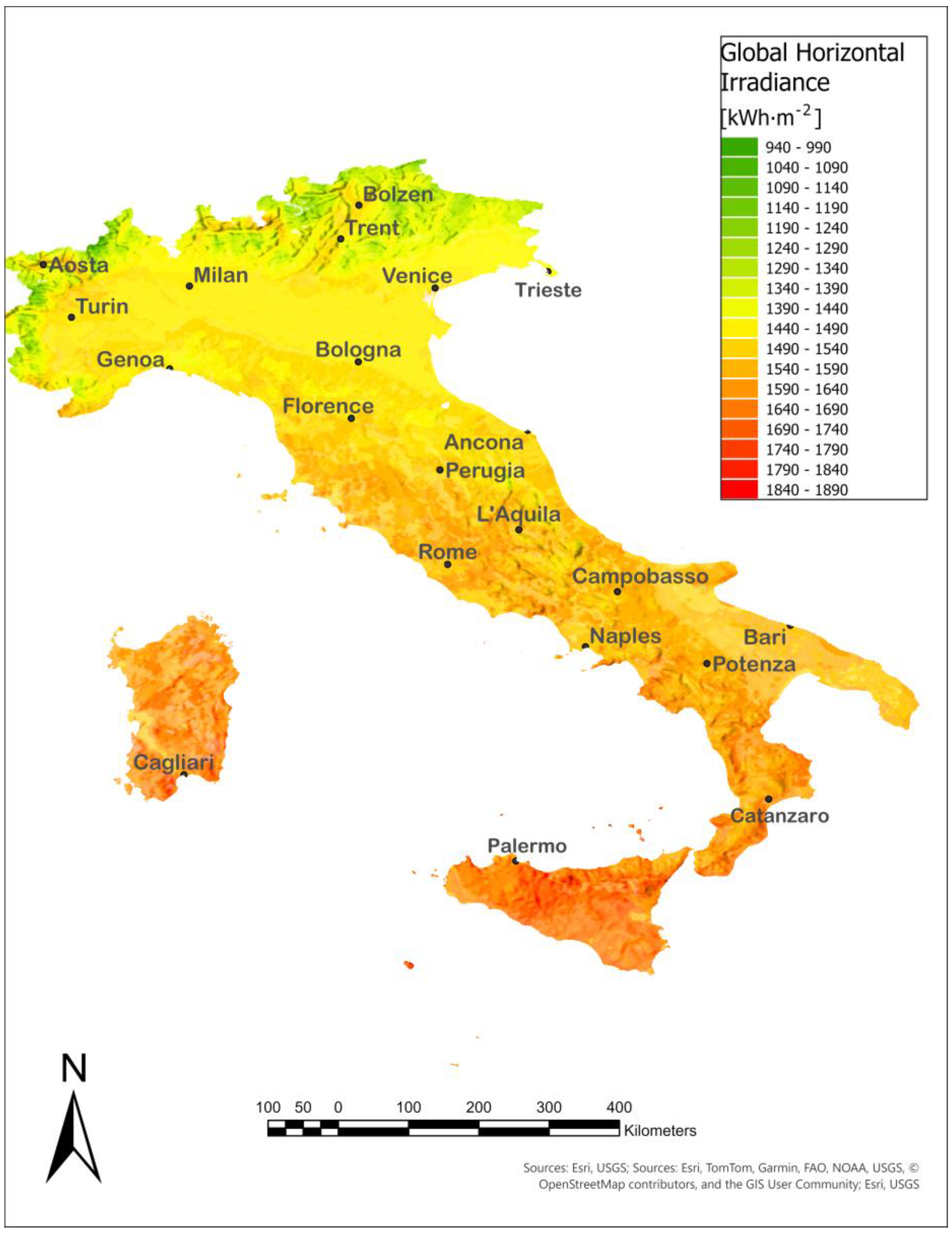
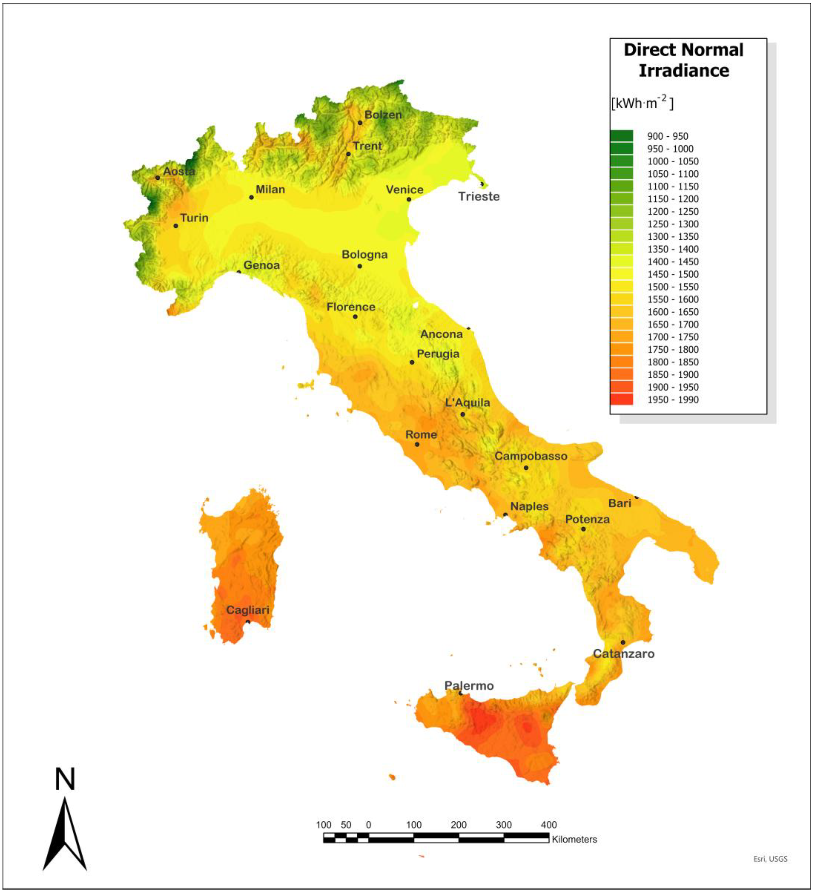
In this work, the EumetSat MSG satellite images of cloud cover with a time frame of 2006–2022 are elaborated with the introduced model. The elaborated images are used to extracted the GHI values from 8093 Italian municipalities and 455 points over the sea. Those data are interpolated with the Kriging method [24] to create solar potential maps over the Italian region. The solar potential of Italy (without San Marino) in terms of the global horizontal (Figure 1) and direct normal irradiance (Figure 2) of daily annual mean values is presented. The maps in this paper are projected onto the WGS84 (World Geodetic System) geographic coordinate system, with the centre of the map at 12°51′6″ E and 41°14′26″ N, using the ArcGIS Pro 3.5.3 software [25].

The spatial distribution of GHI over Italy exhibits a moderate variability, with most values concentrated around approximately 1547 kWh·m⁻² and a relatively narrow dispersion (with standard deviation of 138 kWh·m⁻²). The distribution of the entire spatial domain is close to symmetric, where small differences between the mean and median values are indicated (with a median value of 1528 kWh·m⁻²), suggesting the absence of strong skewness in the dataset. The majority of the GHI values over the entire territory falls within the 1400–1700 kWh·m⁻² range, which corresponds to the dominant yellow–orange classes visible in the map. Lower irradiance values (<1300 kWh·m⁻²) are limited to the restricted areas, mainly associated with the alpine and northern regions, whereas the highest values (>1700 kWh·m⁻²) are concentrated in southern Italy and the major islands. Overall, the spatial distribution confirms a clear north–south gradient and highlights the predominance of medium-to-high solar resource availability across the country.

The spatial distribution of the DNI presented in Figure 2 shows a clear latitudinal gradient and a slightly higher variability compared to GHI, with values generally centered around approximately 1580 kWh·m⁻² and a standard deviation of about 152 kWh·m⁻². The distribution is nearly symmetric, as indicated by the close agreement between mean (1581 kWh·m⁻²) and median values (1567 kWh·m⁻²), suggesting a balanced spread of irradiance across the territory. Most areas fall within the 1450–1750 kWh·m⁻² range, corresponding to the dominant yellow–orange classes observed over central and southern regions. Lower DNI values (<1300 kWh·m⁻²) are mainly confined to northern and alpine areas, where increased cloud cover and complex topography reduce direct solar availability. In contrast, the highest values (>1750 kWh·m⁻²) are concentrated in southern Italy and the major islands, particularly Sicily and Sardinia. Compared with GHI, DNI exhibits a slightly broader spatial dispersion and a stronger sensitivity to regional atmospheric and topographic conditions, reinforcing the complementary role of the two indicators in assessing the solar resource potential.

The predominant values of the annual mean DNI in Figure 2 represent the solar potential becoming profitable for CSP technologies, starting from the latitude of 42° to the south (North Hemisphere), where values higher than 1800 kWh·m⁻² are needed. This value is just a starting point for fast decision-making, where additional studies are needed in CSP site selection in terms of annual distribution and typical meteorological year (TMY) of DNI values. PV solar technologies have the important advantage in using all solar components expressed in terms of GHI, where profitable applications could be found at any latitude. The site selection of the solar power plant is crucial to the design, size, technology, and estimate of power production.

Maps derived from satellite imagery and validated against ground measurements show deviations of approximately 4–6% for monthly mean daily GHI values. Larger discrepancies are observed at higher temporal resolutions, reaching up to 10% for daily data and 20% for hourly data [26]. The average approximation error obtained in this study is consistent with the performance of MSG/SEVIRI-based Heliosat products reported in the literature. For example, Thomas et al. [27] reported relative biases within ±5% and mean relative root mean square error (RMSE) values of approximately 10% for daily GHI when validated against baseline surface radiation network (BSRN) ground measurements. These results confirm the reliability of the adopted methodology and support its suitability for the automated estimation of solar radiation across Italy.

3.2. Solar Potential for the Locations of Interests

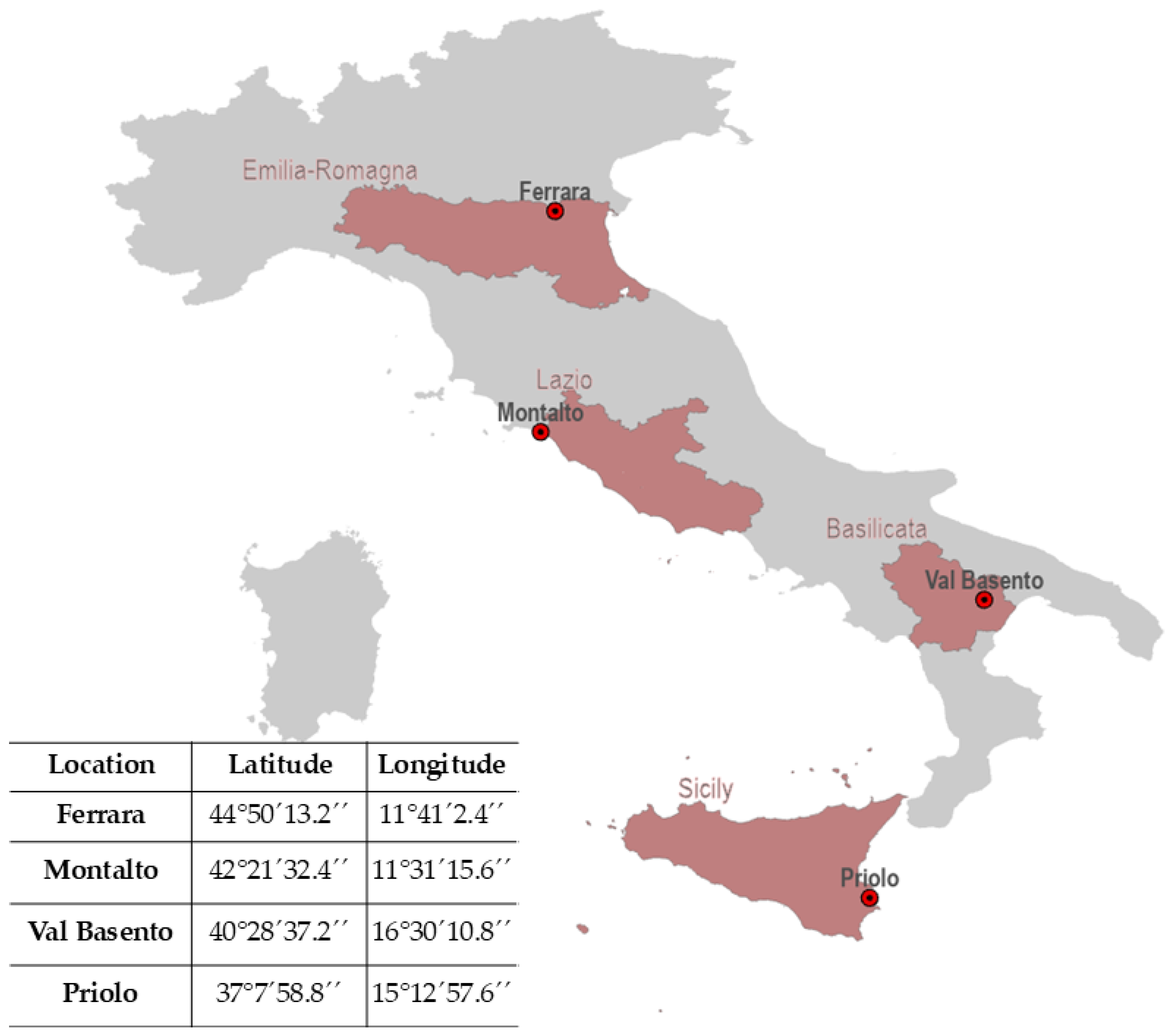
The spatial distributions shown in Figure 1 and Figure 2 for both GHI and DNI indicate favourable solar conditions across large portions of the Italian territory, highlighting the significant potential for effective solar energy exploitation. In the following section, the solar resource availability is analyzed for four representative Italian locations selected to capture regional differences in geographical setting, surface area, orography, population density, and industrial development. The selected case study sites are presented and summarized in Figure 3. The selection of power plant locations was individuated in industrial land use area slightly bigger than a football field of 400 × 300 m, with flat surfaces (needed especially for CSP). Monthly mean values, annual totals, and irradiance duration curves for both GHI and DNI were derived from an irradiance database developed through the processing of the satellite observations acquired from the EUMETSAT and covering the period of 2006–2022. These data are subsequently used to evaluate and compare the performance potential of both CSP and PV technologies at the selected locations.

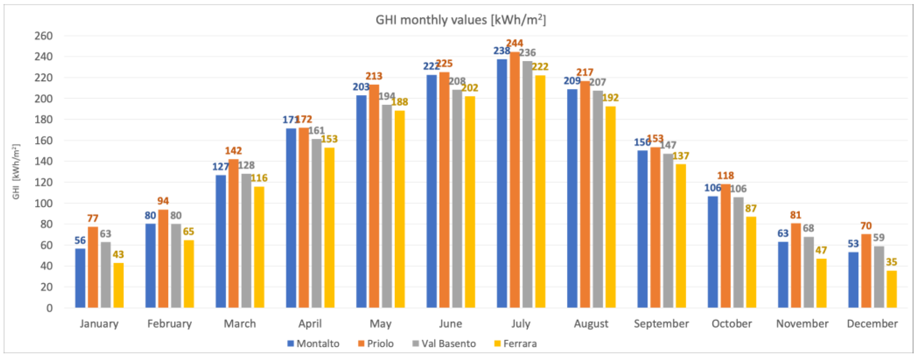
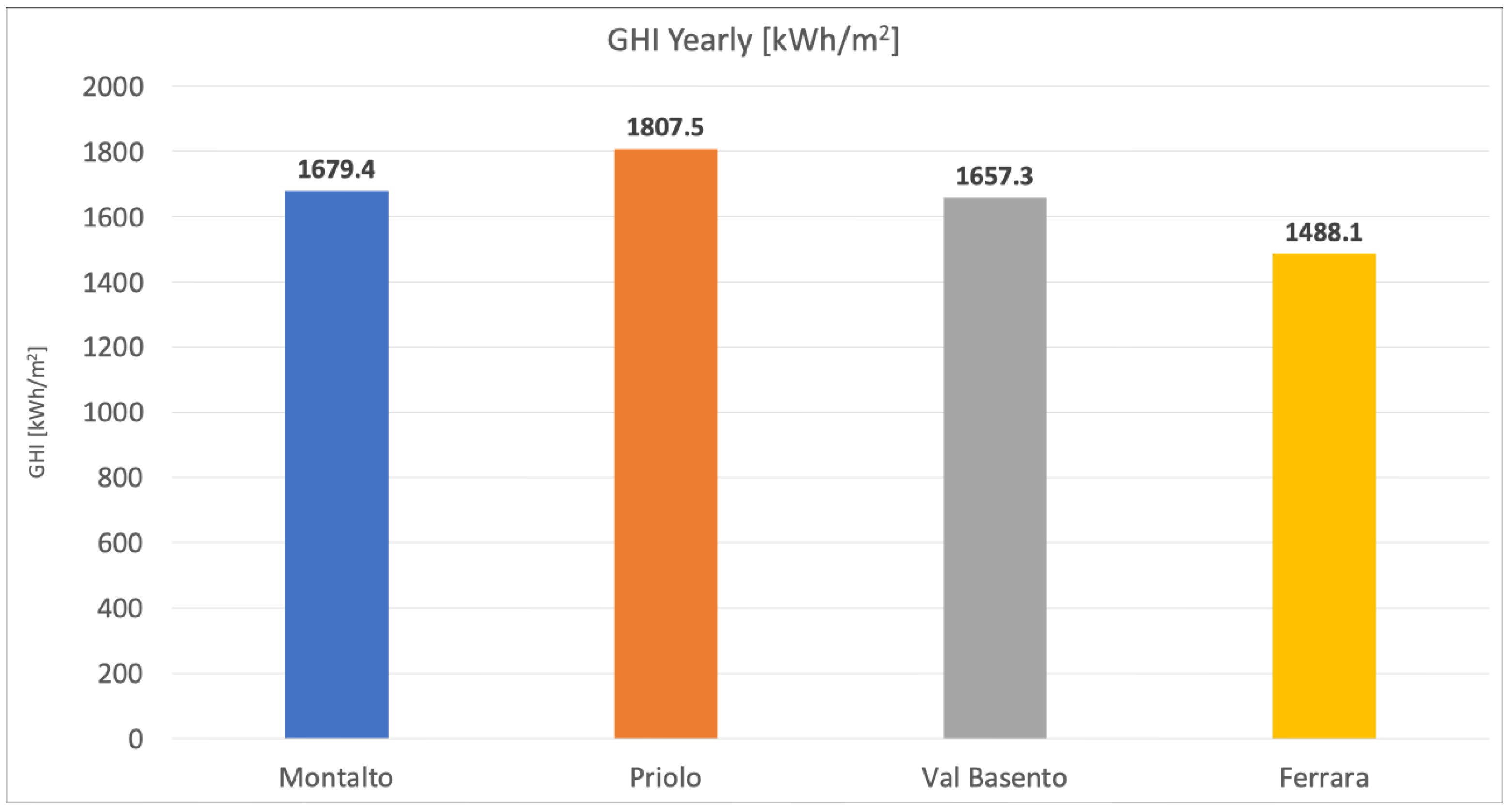
In Figure 4, the chart of monthly and annual GHI values for Montalto, Priolo, Val Basento, and Ferrara for the period of 2006–2022 is shown. All locations follow a similar seasonal trend, with lower irradiation in winter (January–February and November–December) and a steady increase toward summer, peaking between June and July. Priolo and Montalto generally record the highest GHI values throughout the year, indicating stronger solar potential, while Ferrara consistently shows the lowest values, especially in the winter months. Overall, the data highlight a strong summer solar resource and noticeable regional differences in annual solar availability.

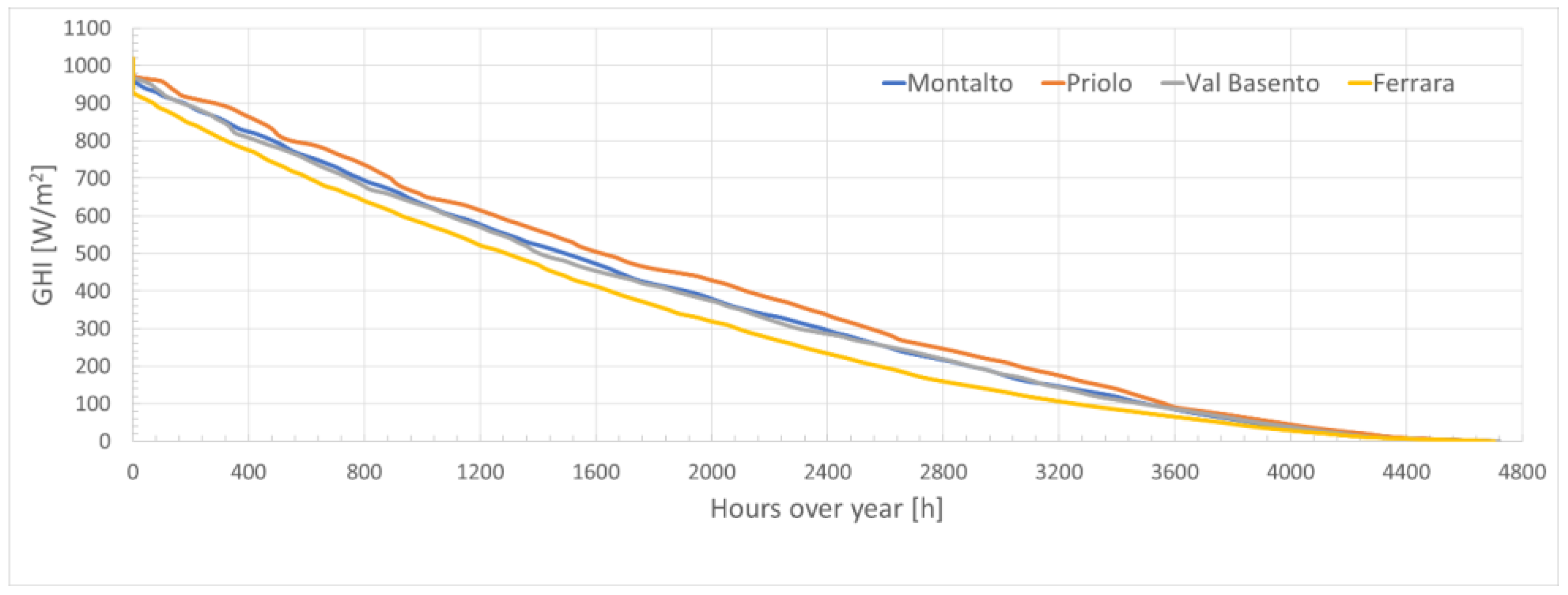
Figure 5 presents the duration curves of GHI for four selected locations, obtained by sorting hourly GHI values in a descending order over the year. Priolo consistently exhibits the highest irradiance levels across most of the distribution, followed by Montalto and Val Basento, while Ferrara shows systematically lower values, particularly at high and medium irradiance ranges. The smooth and nearly parallel decay of the curves indicates similar temporal variability among the sites, whereas the vertical separation reflects persistent regional differences in solar resource availability. At low irradiance levels (right tail of the curves), all locations converge toward near-zero values, corresponding to nighttime and low-sun conditions.

The combined analyses of monthly GHI distributions, annual totals, and duration curves provide a consistent assessment of the solar resource across the four locations. All sites exhibit a pronounced seasonal pattern, with maximum irradiation occurring in late spring and summer and minimum values occurring in winter, reflecting the expected annual solar cycle. The duration curves further indicate similar variability and temporal structure among the sites while maintaining a clear ranking in irradiance magnitude. Priolo systematically shows the highest GHI levels across most operating hours, followed by Montalto and Val Basento, whereas Ferrara presents the lowest irradiance values, particularly at high and medium GHI ranges. This ranking is confirmed by the annual cumulative GHI, with yearly totals of approximately 1807.5 kWh·m⁻² for Priolo, 1679.4 kWh·m⁻² for Montalto, 1657.3 kWh·m⁻² for Val Basento, and 1488.1 kWh·m⁻² for Ferrara. Overall, the agreement among the three representations highlights the robustness of the spatial differences in solar availability and supports the suitability of Priolo and Montalto as the most favourable sites for solar energy exploitation.

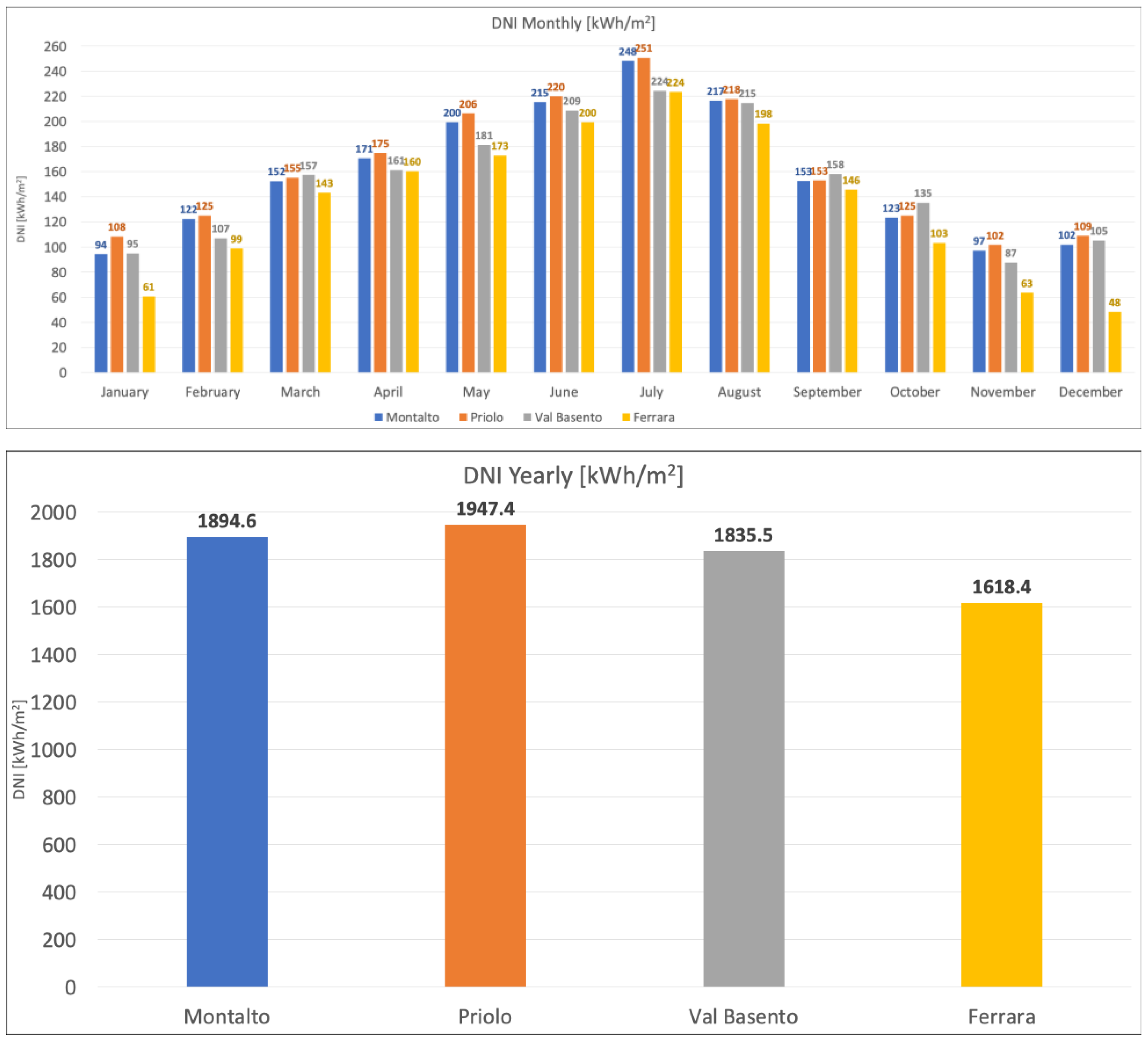
The monthly and annual DNI (Figure 6) values exhibit a clear seasonal cycle and pronounced spatial variability across the four investigated Italian locations (Montalto di Castro, Priolo Gargallo, Val Basento, and Ferrara). At all sites, DNI increases steadily from winter to summer, with maxima occurring between June and July and minima during November–January, reflecting the combined influence of solar elevation and seasonal cloudiness. The southern locations, particularly Priolo and Montalto, consistently record higher monthly values throughout the year, with summer peaks exceeding 240–250 kWh·m⁻², whereas Ferrara exhibits lower values, especially during winter months, indicating greater atmospheric attenuation and cloud cover typical of northern Italy. Val Basento shows intermediate behaviour between these extremes. The annual totals reinforce this gradient, with Priolo presenting the highest DNI (≈1947 kWh·m⁻²), followed by Montalto (≈1895 kWh·m⁻²) and Val Basento (≈1836 kWh·m⁻²), while Ferrara records the lowest value (≈1618 kWh·m⁻²). Overall, the results confirm a distinct north–south increase in DNI solar resource availability, highlighting the superior suitability of southern sites for CSP technologies while still indicating appreciable potential across all regions.

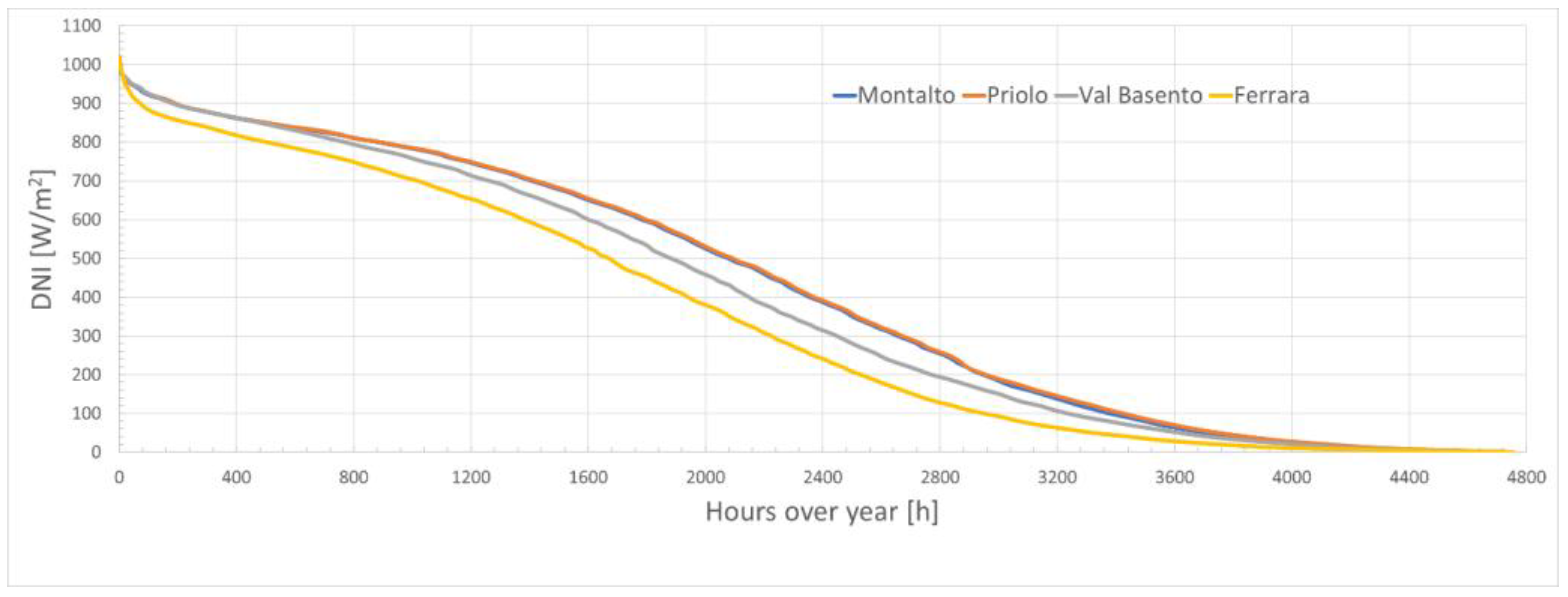
Figure 7 presents the annual cumulative hourly DNI for selected locations, illustrating both the magnitude and persistence of direct solar resource availability throughout the year. The curves are monotonically decreasing, with the highest irradiance levels occurring for a limited number of hours and progressively lower values dominating the remainder of the year. Priolo and Montalto consistently lie above the others across most of the duration, indicating higher DNI intensities sustained for longer periods, whereas Ferrara shows the lowest profile, reflecting more frequent cloud cover and atmospheric attenuation typical of northern regions, while Val Basento exhibits intermediate behaviour. The steeper decline observed for Ferrara suggests fewer high-irradiance hours and shorter periods suitable for operational CSP plants, while the flatter curves for southern locations denote more stable and persistent DNI conditions. Overall, Figure 7 confirms a clear north–south gradient in DNI availability and highlights the superior suitability of southern Italy for concentrating solar technologies that depend on sustained direct irradiance.

Additional meteorological variables, particularly ambient air temperature (T_a) used for PV energy yield calculations, were extracted from the ERA5 climatological reanalysis dataset provided by the Copernicus Climate Change Service [28].

3.3. Real Case Simulation of CSP and PV Plants

The objective of this study is to perform a comparative assessment of CSP and PV technologies based on real case scenarios and consistent design assumptions. Both plants are sized to deliver the same nominal electrical peak capacity of 1 MW, allowing a fair and unbiased comparison in terms of energy production, operational performance, and system behaviour under realistic operating conditions. This approach enables the evaluation of the strengths and limitations of each technology with respect to resource utilization, dispatchability, and potential integration within the power grid. This additional analysis provides insight into the impact of land use constraints on energy yield and highlights the trade-offs between power density, spatial requirements, and overall system performance.

Among CSP configurations, parabolic trough collectors (PCSs) are the most mature and widely deployed technology. In PCSs, solar radiation is concentrated onto a linear receiver tube, where a heat transfer fluid absorbs the thermal energy and transports it to a power block for electricity generation via a conventional thermodynamic cycle. The use of molten salts as a heat transfer and thermal storage medium has gained increasing attention due to their high thermal stability, favourable heat capacity, and capability to enable efficient thermal energy storage at elevated temperatures, thereby improving dispatchability and overall plant flexibility.

In contrast to CSP, crystalline silicon PV technology directly converts solar radiation into electricity through the photovoltaic effect and currently dominates the global PV market owing to its high conversion efficiency, technological maturity, modularity, and rapidly decreasing costs. PV systems exhibit fast deployment, low operational complexity, and scalability from residential to utility-scale installations. However, their power output is inherently intermittent and strongly dependent on instantaneous solar irradiance, typically requiring external energy storage or grid support to ensure supply reliability.

3.3.1. CSP Plant

The CSP technology considered in this study is a PCS system developed by the ENEA, which employs a molten salt mixture as both the heat transfer fluid and the thermal energy storage medium. The adopted molten salt, commonly referred to as solar salt, consists of a binary mixture of sodium nitrate and potassium nitrate (NaNO₃–KNO₃, 60/40 wt%). The system operates at a maximum working temperature of approximately 550 °C, enabling high thermal efficiency and enhanced thermal storage capability.

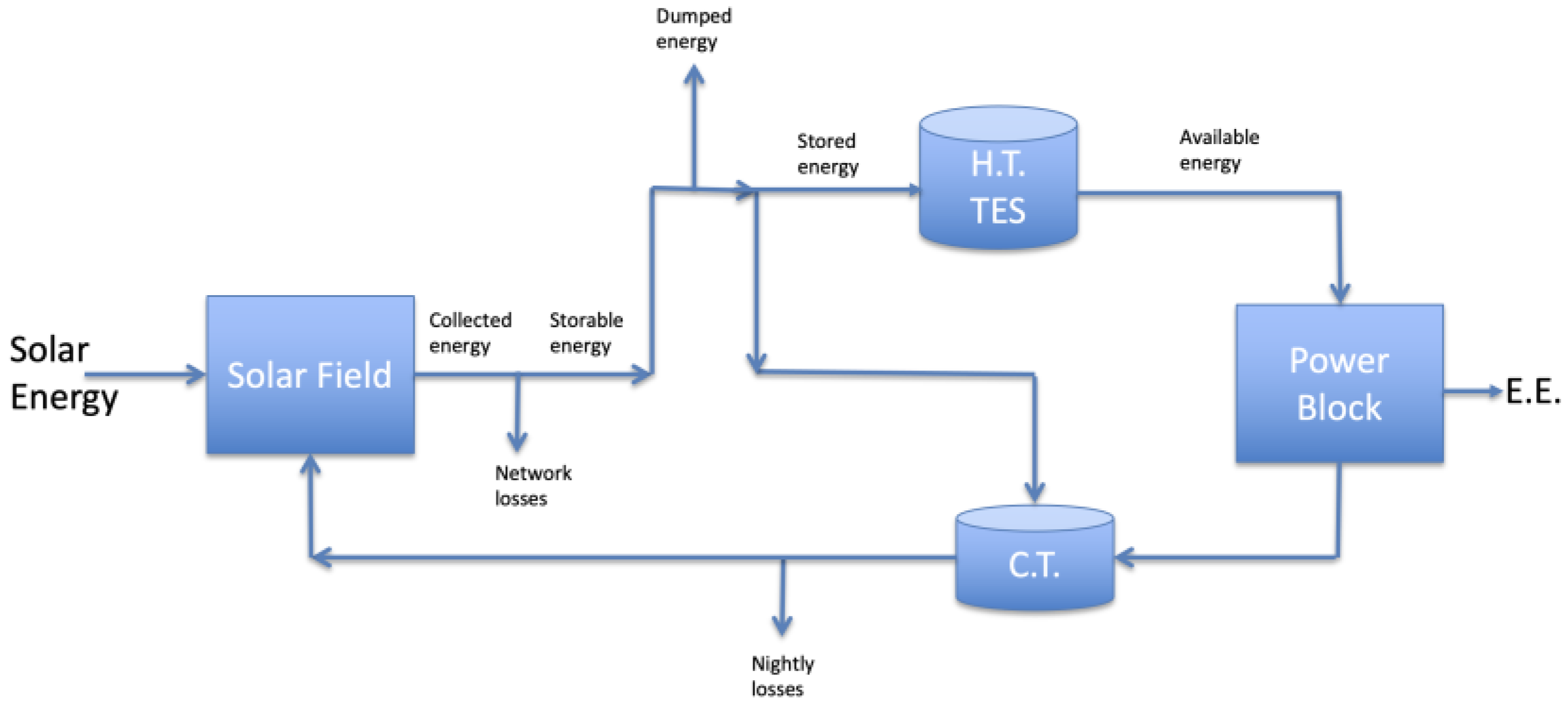
The scheme in Figure 8 presents the energy flow diagram of the CSP plant. The plant configuration includes a solar field of PTCs, a two-tank molten salt thermal energy storage (TES) system with a nominal storage capacity of 8 h at rated power, and a conventional power block based on a steam Rankine cycle. The hot and cold storage tank operating temperatures are approximately 550 °C and 290 °C, respectively. During operation, the molten salt heated in the solar field is directed to the hot storage tank (H.T. TES). Hot molten salt is continuously extracted from the hot tank and supplied to the power block for steam generation; after releasing its thermal energy, the cooled salt is returned to the cold storage tank (C.T.). From the cold tank, the molten salt is then pumped back to the solar field, closing the thermal loop and enabling continuous operation.

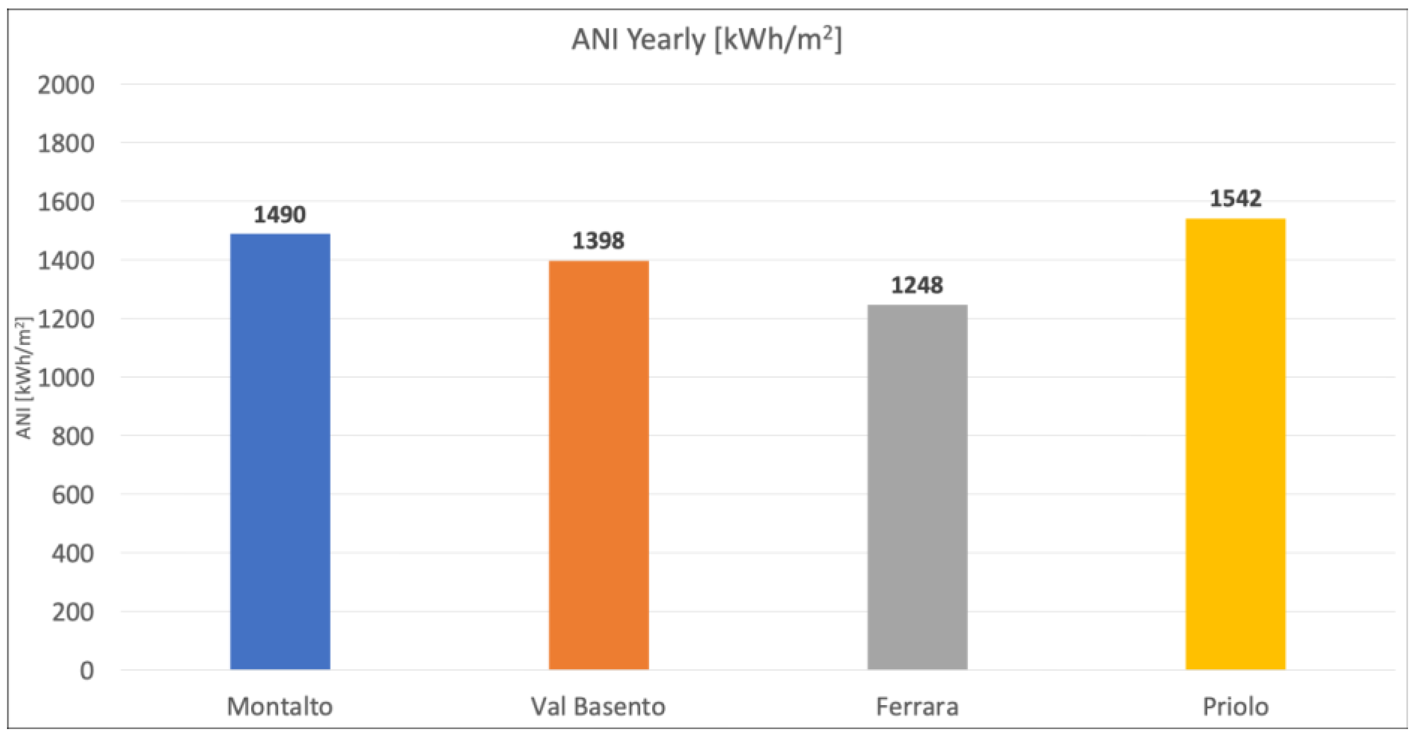
CSP systems exploit only the DNI component of solar radiation, as optical concentration requires collimated sunlight to achieve effective focusing onto the receiver. However, not all the available DNI is effectively intercepted and converted by the collector. The useful radiation is commonly expressed as the aperture normal irradiance (ANI), which represents the fraction of DNI projected onto the collector aperture and effectively contributing to thermal energy generation. ANI depends on several factors, including the solar incidence angle and collector orientation, shading, and end losses [29]. Once the annual hourly profile of ANI is determined, it is used as the primary input for the simulation of the plant productivity and energy yield. The main assumptions adopted for the linear parabolic trough the CSP plant are summarized in

Table 1. Linear parabolic through CSP plant characteristics.

PEL Nominal Electrical Power	1 MWe
$\mathrm{\eta }$th Rankine cycle	0.38
Pth nominal thermal power to power block	2.65 MWth
Thermal fluid	Solar salts (290–550 °C)
$\mathrm{\eta }$opt optical efficiency [29]	0.758
$\mathrm{\eta }$th thermal efficiency [29]	0.8827 (for ANI of 800 W·m−2)
SM solar multiple	2.5
Type of collector and receiver tube [29]	ENEA
ANI ref design	800 W·m−2

below.

The active aperture area of the solar field is calculated assuming a collector loop length of 600 m, a parabolic trough aperture width of 5.9 m, and a row spacing (pitch) of 15 m. The annual ANI for the locations selected in this study is shown in Figure 9. The ANI was calculated assuming a north–south orientation of the solar field with east–west tracking.

The active reflective surface area of a single loop of the ENEA solar collector is 3398.4 m². Under these assumptions, the required number of loops is calculated from the following energy balance:

$$P_{loop}=A_{loop}·{ANI}_{ref}·{\eta }_{th}·{\eta }_{opt}=3398.4·800·0.8827·0.758=1.82 {\mathrm{M}\mathrm{W}}_{\mathrm{t}\mathrm{h}}$$

$$N_{loop}={\displaystyle \frac{P_{th}}{P_{loop}}}·SM={\displaystyle \frac{2.65}{1.82}}·2.5=3.65$$

After rounding up to the nearest integer, the system requires four loops, corresponding to a total active area of 13,363 m². When accounting for the inter-row spacing and auxiliary areas, the corresponding total land occupation is estimated to be approximately 50,000 m².

For the CSP plant simulations, the DNI values are first converted into ANI. The resulting ANI time series is then used as input for the CSP performance model described in [29,30], which calculates the thermal power collected by the solar field, the charging and discharging behaviour of the TES, and the electrical power produced by the Rankine cycle power block.

A constant electrical efficiency of 0.38 was assumed for the power block. The thermal energy delivered from the solar field and TES to the power block (2.65 MW_th) is converted into electrical output using this efficiency. By integrating the hourly electrical power production over the year, the annual electricity generation is obtained. The capacity factor (CF) is then calculated as the ratio between the actual annual electrical energy produced and the energy that would be generated if the plant operated continuously at its nominal power.

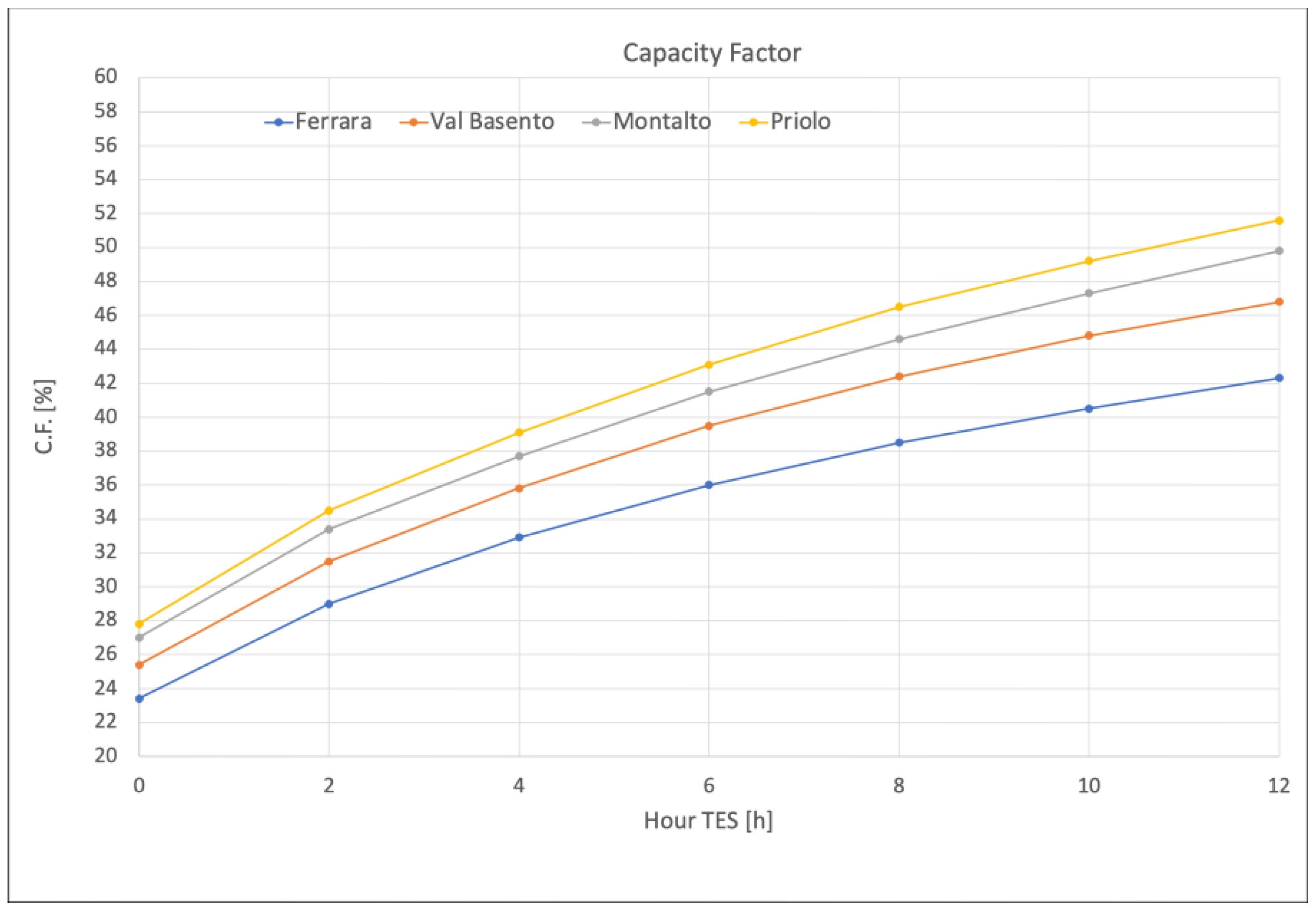
The simulations were performed considering storage capacities of 0, 2, 4, 6, 8, 10, and 12 h. Figure 10 reports the annual CF as a function of TES hours for the four investigated locations: Ferrara, Val Basento, Montalto, and Priolo. For all sites, the CF increases monotonically with increasing TES capacity, confirming the beneficial role of thermal storage in enhancing plant utilization and dispatchability. Locations characterized by higher solar availability, such as Priolo and Montalto, systematically exhibit higher CF values compared with Val Basento and Ferrara. At zero storage, the CF ranges from approximately 23.4% in Ferrara to 27.8% in Priolo, while for 12 h of TES, it increases up to about 42.3–51.6%, depending on the site. This trend indicates that larger storage capacities reduce energy curtailment and enable a more effective exploitation of the available solar resource, resulting in improved annual performance.

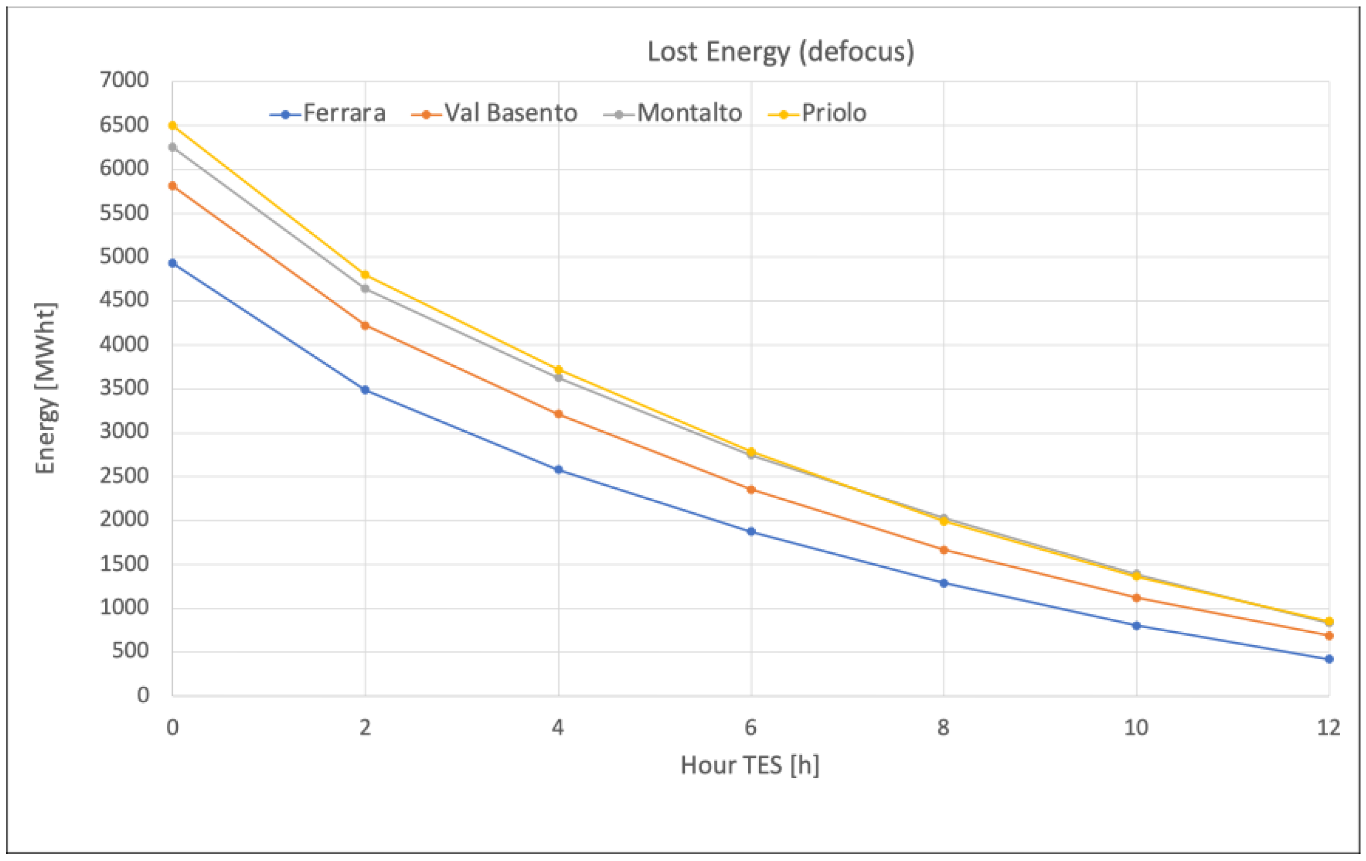
Figure 11 shows the annual thermal energy lost due to solar field defocusing, caused by an overfilled TES system, for the investigated locations: Ferrara, Val Basento, Montalto, and Priolo. When the storage capacity is insufficient to accommodate the collected thermal energy, part of the solar field is defocused to avoid exceeding TES and power block limits, resulting in energy curtailment. For all sites, the lost energy decreases monotonically with increasing TES capacity, indicating that larger storage sizes effectively mitigate defocusing events and associated thermal energy losses. At zero storage, the annual curtailed energy reaches its maximum, ranging approximately from 4933 MW_th in Ferrara to about 6500 MW_th in Priolo, reflecting the different solar resource availability among the locations. As the TES capacity increases up to 12 h, the lost energy is significantly reduced for all sites, falling below approximately 400–850 MW_th. Locations with higher solar resource, such as Priolo and Montalto, exhibit systematically higher defocused energy, consistent with their higher potential energy yield.

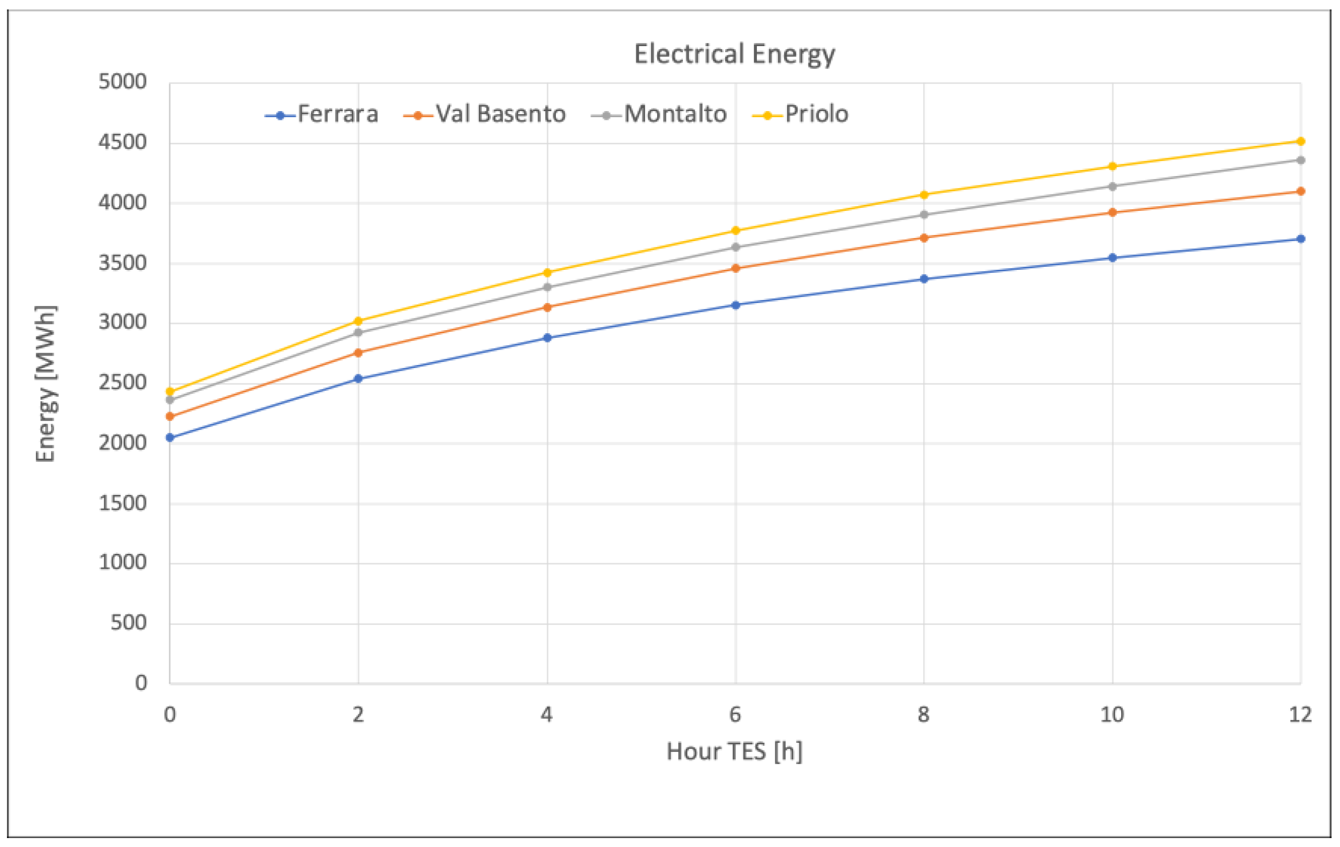
Figure 12 presents the annual electrical energy production as a function of TES hours for the four investigated locations. For all sites, the electrical output increases monotonically with increasing TES capacity, highlighting the positive impact of thermal storage on the exploitation of the available solar resource and on the reduction in energy curtailment. Sites characterized by higher solar irradiance, such as Priolo and Montalto, consistently exhibit higher electricity production compared with Val Basento and Ferrara across the entire range of TES capacities. At zero storage, the annual electrical energy ranges approximately from 2 GWh in Ferrara to about 2.4 GWh in Priolo, while at 12 h of TES, it increases up to approximately 3.7–4.5 GWh, depending on the location. The progressive flattening of the curves at higher TES values suggests diminishing marginal gains in electrical output as storage capacity increases, indicating a trade-off between storage size and achievable energy benefits.

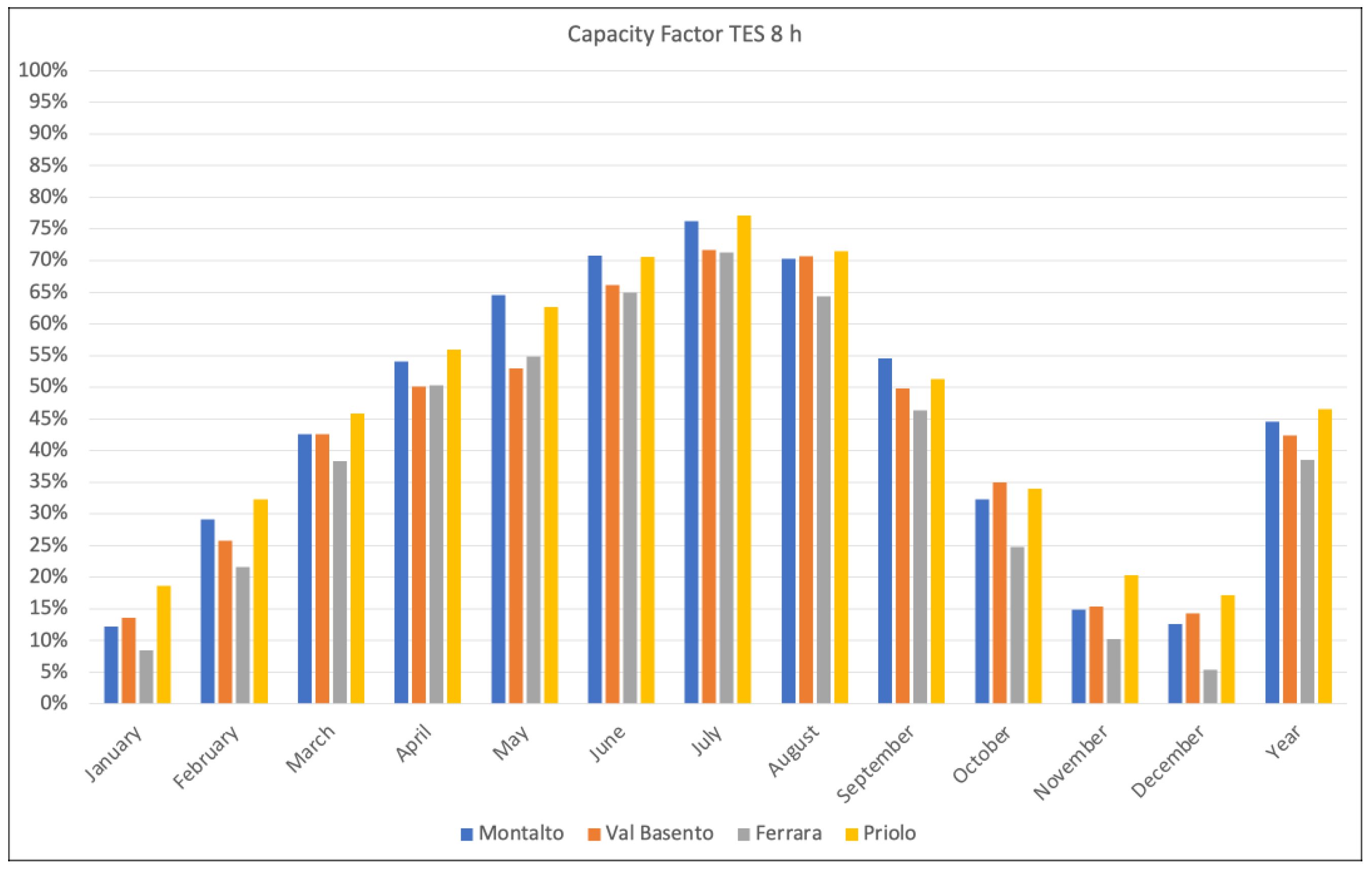
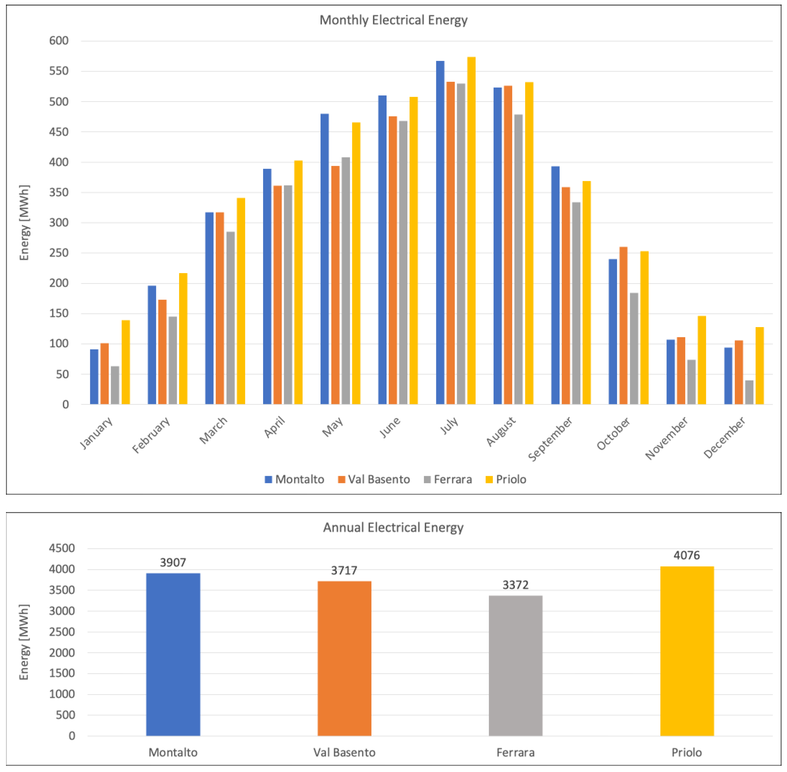
For the subsequent analyses, the results corresponding to a TES capacity of 8 h are adopted as the reference case. Figure 13 and Figure 14 present, respectively, the monthly CF and the monthly and annual electricity generation of the CSP plants equipped with 8 h of TES for the four investigated locations (Montalto, Val Basento, Ferrara, and Priolo). A clear seasonal trend is observed at all sites, with minimum values occurring during the winter months (January–February and November–December) and maximum values in the summer (June–August), reflecting the strong dependence on direct normal irradiance and daylight availability. This seasonal behaviour is consistently reflected in both the CF and the electricity generation profiles. Among the analyzed locations, Priolo systematically exhibits the best performance throughout the year, reaching peak capacity factors close to 77–78% during the summer months and maintaining relatively high values also during the shoulder seasons. Accordingly, it shows the highest monthly electricity production, with peak values of about 570–530 MWh in July–August, and the largest annual generation of approximately 4076 MWh. Montalto and Val Basento display similar trends and intermediate performance, with summer peak CF in the range of about 70–76% and maximum monthly generation between approximately 520 and 565 MWh. On an annual basis, Montalto produces about 3907 MWh, while Val Basento reaches around 3717 MWh. Ferrara consistently records the lowest performance, particularly during the winter months, both in terms of the capacity factor and electricity generation, with a total annual production of approximately 3372 MWh, due to less favourable solar resource conditions. Overall, the comparison confirms that the site location plays a key role in determining plant performance: despite identical plant configurations, differences in solar resource availability translate into significant variations in both the capacity factor and electricity output. The presence of an 8 h thermal energy storage system helps mitigate seasonal variability and enables relatively high utilization during periods of moderate irradiance; however, winter months remain the main limiting factor for achieving high CF values and energy production.

3.3.2. PV Plant

PV technology investigated in this study is based on a monocrystalline silicon module, model HiKu6 Mono Passivated Emitter and Rear Cell (PERC) CS6W-550MS manufactured by Canadian Solar (Kitchener, ON, Canada), with a rated peak power of 550 W under standard test conditions (STC irradiance of 1000 W·m⁻², spectrum AM 1.5, and cell temperature of 25 °C). The module employs the PERC technology, which improves carrier collection and enhances conversion efficiency. The electrical, mechanical, and temperature characteristics of the selected PV module are reported in

Table 2. Photovoltaic plant characteristics [31].

Electrical Data (STC)
Nominal max. power (Pmax)	550 W
Module efficiency	21.5%
Open-circuit voltage (Voc)	49.6 V
Short-circuit current (Isc)	14.00 A
Mechanical Data
Cell type	Mono-crystalline
Dimensions	2261 × 1134 × 30 mm
Temperature Characteristics
Temperature coefficient (Pmax)	−0.34%/°C
Temperature coefficient (Voc)	−0.26%/°C
Temperature coefficient (Isc)	0.05%/°C
Nominal module operating temperature	41 ± 3 °C

[31].

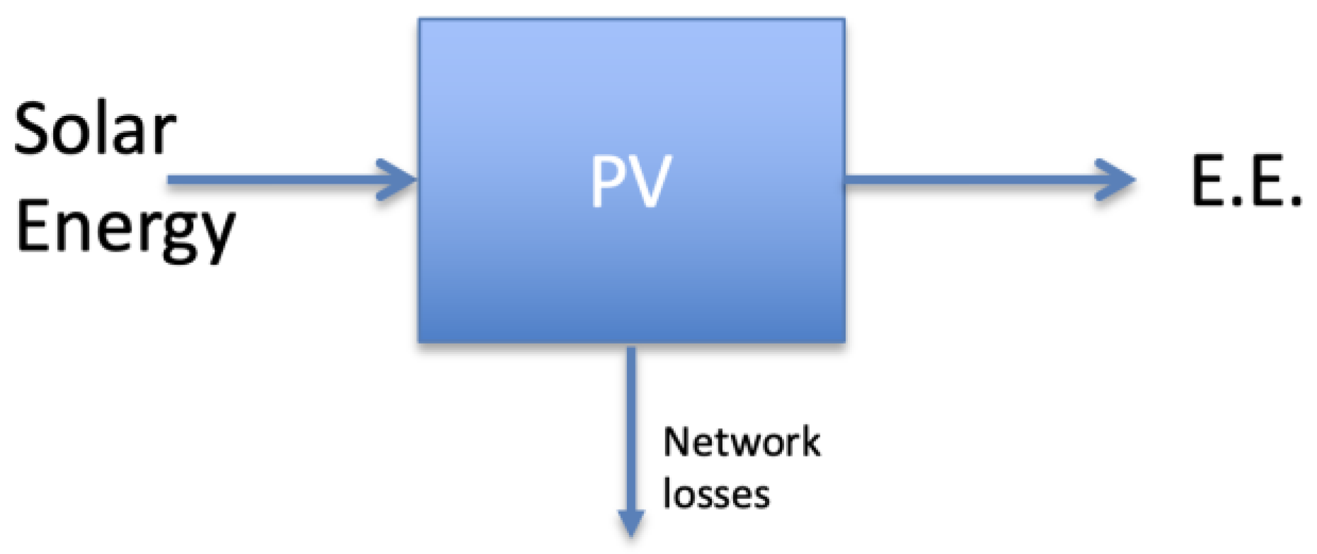
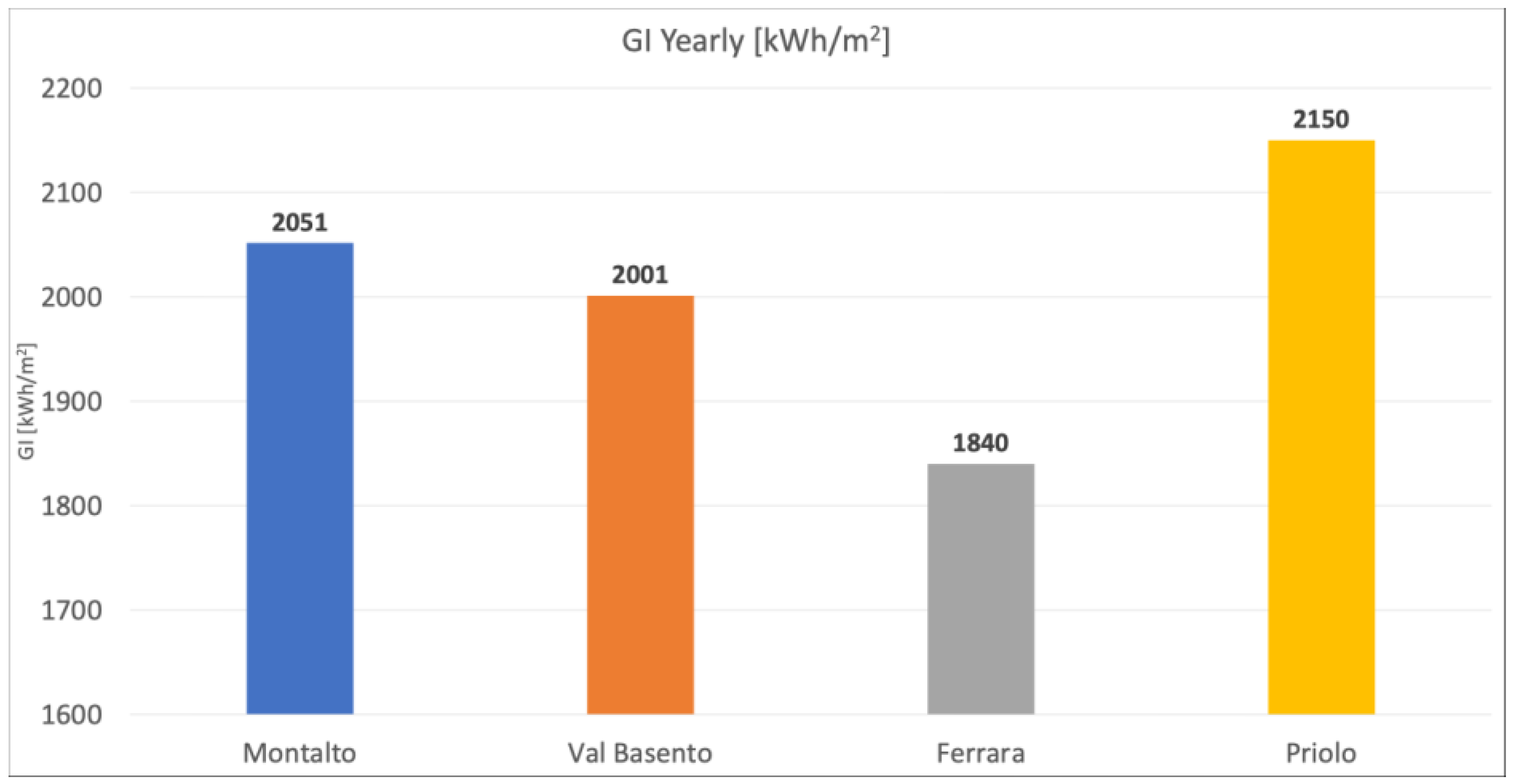
Figure 15 presents the conceptual scheme of the PV system, showing the conversion of solar irradiance into electrical energy (E.E.) and the associated network losses during transmission. Accordingly, the electrical energy conversion is governed by the plane-of-array (POA) irradiance, also referred to as the global irradiance incident on the module surface (GI), rather than by the direct normal irradiance alone. The POA irradiance is obtained by transposing GHI into the tilted plane of the PV module using the established transposition models [32], which account for the geometric relationship between the sun position and the module orientation. The total incident irradiance is calculated as the sum of the DHI, DiffHI, and ground-reflected components, with the latter depending on the surface albedo. Additional optical effects, including the angle-of-incidence modifier (IAM) and shading losses, are considered to evaluate the fraction of radiation effectively absorbed by the module. The annual GI on the PV module plane for the selected locations is shown in Figure 16. The GI was calculated assuming a single-axis tracking system with a north–south axis orientation and east–west rotation, analogous to the tracking configuration adopted for the CSP layout. A backtracking strategy was implemented to mitigate row-to-row shading losses during low solar elevation angles, in accordance with the methodology proposed by the National Renewable Energy Laboratory (NREL) [33,34]. Backtracking slightly reduces the instantaneous tracking angle with respect to the ideal sun-pointing position in order to prevent mutual shading between adjacent tracker rows, thereby improving the overall energy yield.

For the estimation of the PV E.E. production, an assumption in design was that the installed PV peak power was set equal to the nominal electrical capacity assumed for the CSP plant. This scenario allows a consistent comparison of energy yield under equivalent power-based and area-based constraints. A ground coverage ratio (GCR) of 0.47 was assumed. The GCR is defined as the ratio between the total active PV module area and the total land area occupied by the PV plant, and it directly affects row spacing, shading losses, and land use efficiency. In addition, a constant performance ratio (PR) of 0.82 was considered. The PR represents the overall system efficiency by accounting for all non-ideal losses between the incident solar irradiance and the delivered E.E., including temperature effects, inverter losses, soiling, wiring, mismatch, and availability losses.

Assuming a PV field peak capacity of 1 MW_e, a total of 1818 modules are required, resulting in an overall active module area of 4654 m², considering an active area of 2.56 m² per module. By adopting a GCR of 0.47, the corresponding land area required for the PV plant is estimated to be 9902.3 m². The electrical output of the PV system is estimated using the PV performance model described in [35]. In this model, the electrical power production depends primarily on the hourly profile of the GI and the hourly profile of the ambient temperature (T_a). The GI determines the amount of solar energy available for conversion, while the ambient temperature affects the operating temperature of the PV cells and therefore the module efficiency. By integrating the hourly electrical power over the year, the monthly and annual electricity production and the corresponding capacity factor are obtained.

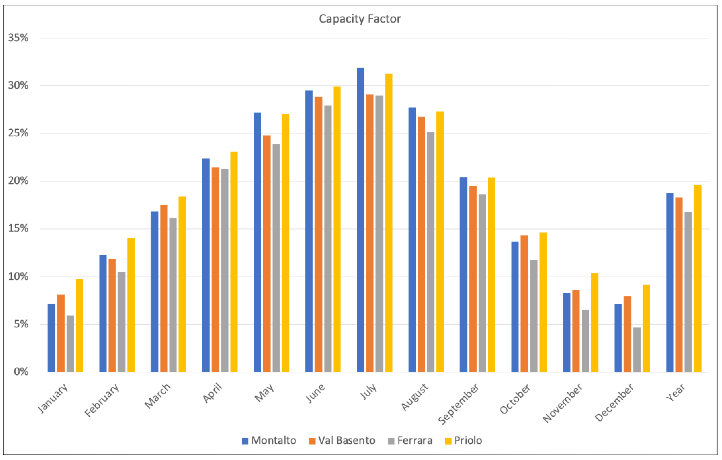
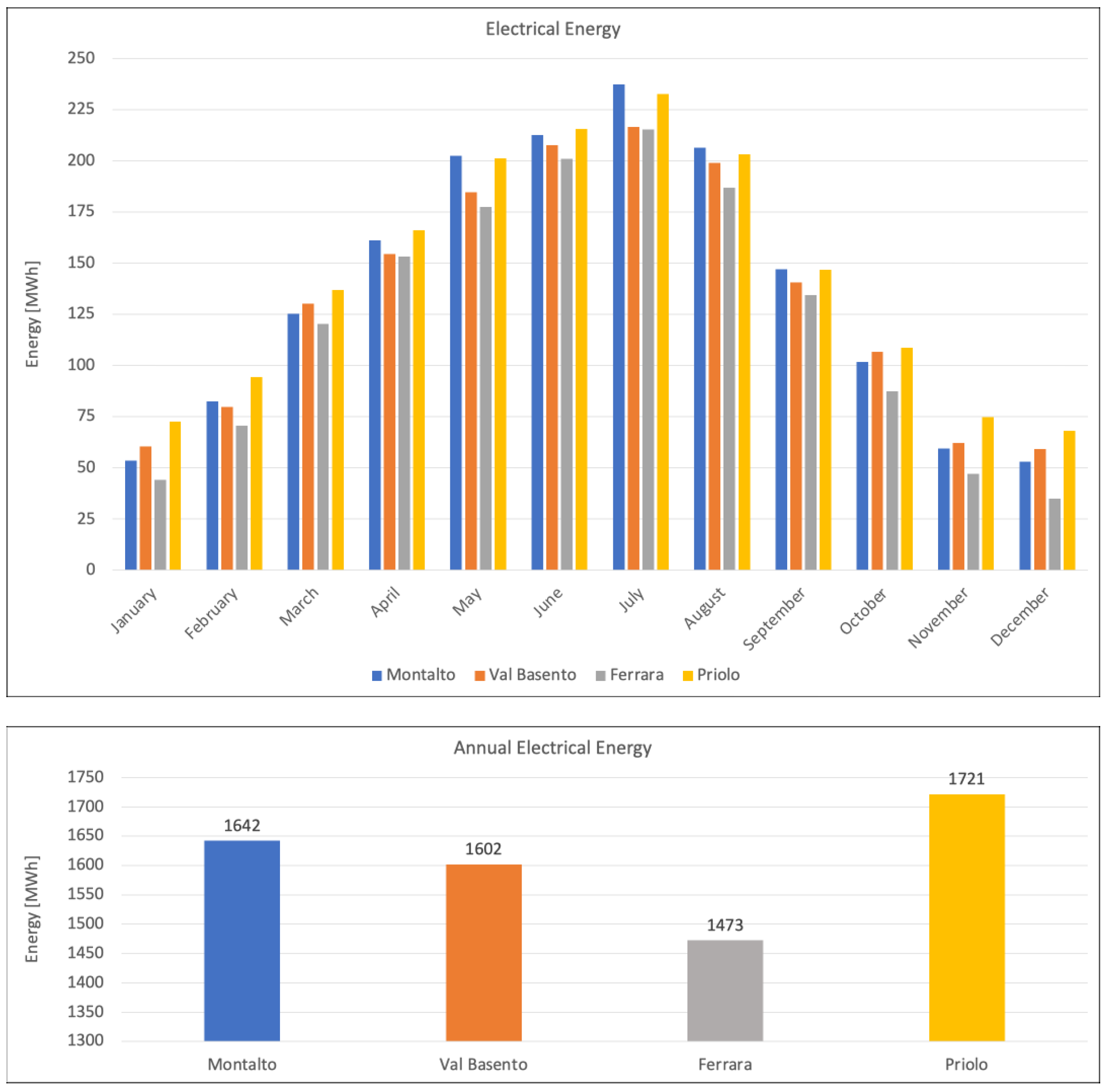
Figure 17 and Figure 18 provide a consistent comparison between the monthly and annual CF and the corresponding E.E. production of a 1 MW PV plant for the four investigated locations (Montalto, Val Basento, Ferrara, and Priolo). In all cases, the two indicators exhibit the same seasonal behaviour, with a progressive increase from winter to summer, peak values in June–July, and a decline during autumn and winter. This confirms the strong dependence of PV performance on solar irradiance availability and daily sunlight duration. Priolo systematically shows the highest performance among the analyzed sites, achieving the largest monthly CF (exceeding 31% in July) and the highest monthly E.E. generation (about 230–235 MWh), which results in the maximum annual E.E. of approximately 1721 MWh. Montalto and Val Basento present intermediate and comparable performance levels. Montalto slightly outperforms Val Basento in terms of peak CF and annual E.E. (about 1642 MWh versus 1602 MWh), while Val Basento shows marginally higher values during some winter and transitional shoulder months. Ferrara consistently records the lowest CF throughout the year, particularly in winter, leading to reduced monthly E.E. production and the lowest annual energy yield (about 1473 MWh). The close agreement between the CF profiles and E.E. trends indicates that energy production scales almost linearly with plant utilization for a fixed installed capacity. Minor deviations between the two metrics can be attributed to differences in month length and operational conditions. Overall, the comparison highlights the significant impact of geographical location on PV plant performance and confirms that southern sites, such as Priolo, benefit from higher and more stable solar resources, whereas northern sites, such as Ferrara, experience lower utilization rates and reduced annual energy output.

4. Discussion

This work compares the technical and economic performance of CSP plants equipped with 8 h of TES and a 1 MW PV plant across four representative Italian locations—Montalto, Val Basento, Ferrara, and Priolo. For both technologies, the results highlight a pronounced seasonal behaviour, with reduced CF and E.E. generation during winter months and peak values in summer, reflecting the strong dependence on solar resource availability and daylight duration. In all cases, the relative ranking of site performance remains consistent, with Priolo exhibiting the highest utilization and energy yield and Ferrara the lowest.

Despite this common trend, significant differences emerge between the two technologies. The CSP plant benefits from dispatchable operation enabled by the TES, delivering an almost constant electrical power output equal to its nominal capacity of 1 MWe during operating periods. This characteristic allows CSP to partially decouple electricity generation from instantaneous solar availability. In contrast, the PV plant operates in a fully non-dispatchable manner, with power output directly linked to real-time GI. As a result, PV generation is inherently variable, with maximum instantaneous power values of approximately 0.89 MW in Priolo and 0.85 MW in Ferrara, and zero production under low irradiance conditions.

The presence of the TES significantly enhances CSP performance by mitigating short-term and seasonal variability and enabling relatively high utilization during transitional months in shoulder periods. This leads to peak summer CF approaching 78% and annual E.E. production exceeding 4 GWh at the best-performing site. Nevertheless, winter months remain the primary limiting factor for CSP, as reduced DNI limits both solar field efficiency and storage charging. PV systems exhibit stronger temporal variability, with peak CF below approximately 31% and annual electricity generation ranging between about 1.47 and 1.72 GWh, depending on the location.

A notable outcome of the analysis is that the north–south geographical location gradient in energy production is more pronounced for CSP than for PV. When comparing Priolo (southern site) and Ferrara (northern site), CSP annual E.E. generation decreases by approximately 17.3%, whereas the corresponding reduction for PV is about 14.4%. This difference is primarily attributed to the stronger dependence of CSP on DNI, which exhibits higher sensitivity to latitude, atmospheric conditions, and cloud cover. PV systems, by contrast, can exploit both global solar radiations, resulting in a comparatively attenuated geographical performance gap.

Land use further differentiates the two technologies. The CSP plant, including the solar field and TES, requires approximately 50,000 m², while the PV plant with the same nominal electrical capacity occupies about 10,000 m². When normalized by occupied surface, the specific energy density ranges from about 67.5 to 81.5 kWh·m⁻²·year⁻¹ for CSP and from approximately 147.3 to 172 kWh·m⁻²·year⁻¹ for PV systems, indicating that PV systems achieve more than twice the annual energy production per unit area. This higher land use efficiency makes PV systems particularly attractive in contexts where land availability is limited, whereas CSP requires careful spatial planning.

From an economic perspective, the levelized cost of electricity (LCOE) analysis confirms that, under typical Europe/Mediterranean cost assumptions [36], PV achieves substantially lower LCOE values than CSP with 8 h TES, mainly due to its significantly lower capital and operating costs. However, the LCOE alone does not fully capture the system value of CSP, which provides dispatchability, operational flexibility, and improved grid compatibility. The site dependence observed in E.E. production is also reflected in economic performance: moving from Priolo to Ferrara increases LCOE by approximately 17% for PV and about 20% for CSP, further highlighting the stronger sensitivity of CSP economics to solar resource quality.

5. Conclusions

This study provided a comprehensive comparison of CSP plants with 8 h of TES and PV plants of equal nominal capacity across different geographical locations. The results demonstrate that both technologies are strongly influenced by site-specific solar resources, with southern locations consistently outperforming the northern ones in terms of the capacity factor, electricity generation, and economic indicators.

CSP technology with TES achieves higher utilization rates and nearly constant rated power output during operation, offering dispatchable electricity and enhanced grid integration capabilities. These advantages come at the expense of higher land occupation and significantly higher LCOE values compared with PV. Moreover, CSP performance exhibits a stronger sensitivity to geographical location due to its reliance on DNI only, resulting in a more pronounced North–South performance gradient. In addition to E.E. power generation, CSP technology is also particularly promising for the supply of medium- to high-temperature heat processes in industrial sites, further broadening its potential role in the decarbonization of hard-to-abate sectors.

PV systems, on the other hand, provide lower-cost electricity and superior land use efficiency, producing more than twice the annual energy per unit area compared with CSP. However, their operation remains intrinsically intermittent and fully dependent on instantaneous solar irradiance, limiting their ability to provide firm and dispatchable power without additional storage or grid support. In addition, the modularity and scalability of PV technology make it particularly suitable for distributed generation and small-scale residential or commercial applications, enabling widespread deployment, simplified installation, and reduced operational complexity.

Conversely, CSP plants are generally more appropriate for large utility-scale installations, where economies of scale can partially offset higher investment costs. Their operation typically requires dedicated infrastructure, centralized layouts, and specialized technical personnel for plant management, maintenance, and control, making them less suited to decentralized or small-scale applications.

Overall, the findings indicate that no single technology is universally optimal. While PV is well suited for cost-effective, space-efficient, and distributed electricity generation, CSP with TES represents a valuable option where dispatchability, system flexibility, higher utilization, and industrial heat supply are required. These results provide useful insights for technology selection, integrated energy planning, and sustainable deployment of solar power systems in Europe and similar regions. In this perspective, hybrid integration of PV and CSP technologies with TES emerges as a particularly promising pathway, as it combines PV technology’s low-cost and land-efficient energy production with CSP’s inherent dispatchability and storage capabilities, thereby enhancing overall system reliability, smoothing power output, reducing curtailment, and improving both the economic and operational performance of future solar-dominated energy systems.

References

1. Intergovernmental Panel on Climate Change (IPCC). AR6 Synthesis Report. In IPCC Synthesis Report 2023; IPCC: Geneva, Switzerland, 2023. [Google Scholar]
2. International Energy Agency (IEA). Renewables 2023; IEA: Paris, France, 2024. Available online: https://www.iea.org/reports/renewables-2023 (accessed on 5 February 2026).
3. IEA COP28 Tripling Renewable Capacity Pledge. Available online: https://iea.blob.core.windows.net/assets/ecb74736-41aa-4a55-aacc-d76bdfd7c70e/COP28TriplingRenewableCapacityPledge.pdf (accessed on 5 February 2026).
4. IEA. Technology Roadmap: Solar Thermal Electricity; International Energy Agency: Paris, France, 2014. [Google Scholar]
5. International Renewable Energy Agency (IRENA). Concentrating Solar Power: Technology Brief; International Renewable Energy Agency: Abu Dhabi, United Arab Emirates, 2012. [Google Scholar]
6. Lovegrove, K.; Stein, W. Concentrating Solar Power Technology; Woodhead Publishing: Cambridge, UK, 2012. [Google Scholar]
7. Kalogirou, S. Solar Energy Engineering: Processes and Systems, 2nd ed.; Academic Press: London, UK, 2014. [Google Scholar]
8. NREL. Concentrating Solar Power Basics; National Renewable Energy Laboratory: Golden, CO, USA, 2018. [Google Scholar]
9. Fernández-García, A.; Zarza, E.; Valenzuela, L.; Pérez, M. Parabolic-trough solar collectors and their applications: A review. Sol. Energy 2010, 84, 1697–1721. [Google Scholar] [CrossRef] [Scilit]
10. NREL. Parabolic Trough Solar Technology Basics; National Renewable Energy Laboratory: Golden, CO, USA, 2003. [Google Scholar]
11. IEA PVPS. Trends in Photovoltaic Applications; International Energy Agency: Paris, France, 2025. [Google Scholar]
12. International Renewable Energy Agency (IRENA). Future of Solar Photovoltaic: Deployment, Investment, Technology, Grid Integration; International Renewable Energy Agency: Abu Dhabi, United Arab Emirates, 2019. [Google Scholar]
13. NREL. Solar Photovoltaic Technology Basics; National Renewable Energy Laboratory: Golden, CO, USA, 2019. [Google Scholar]
14. Green, M.A. Solar Cells: Operating Principles, Technology and System Applications; Prentice Hall: Englewood Cliffs, NJ, USA, 1982. [Google Scholar]
15. Duffie, J.A.; Beckman, W.A. Solar Engineering of Thermal Processes, 4th ed.; Wiley: Hoboken, NJ, USA, 2013. [Google Scholar]
16. Joint Research Centre (JRC). PVGIS—Photovoltaic Geographical Information System; European Commission: Ispra, Italy, 2019. [Google Scholar]
17. Petrarca, S.; Cogliani, E.; Spinelli, F. La Radiazione Solare Globale al Suolo in Italia; ENEA: Rome, Italy, 2000. [Google Scholar]
18. European Commission. The European Climate Law and Fit for 55 Package; European Commission: Brussels, Belgium, 2021. [Google Scholar]
19. Ministero dell’Ambiente e della Sicurezza Energetica. Piano Nazionale Integrato per l’Energia e il Clima (PNIEC); Government of Italy: Rome, Italy, 2024. [Google Scholar]
20. EUMETSAT. EUMETSAT User Data Portal—MSG SEVIRI Satellite Data; EUMETSAT: Darmstadt, Germany, 2026. Available online: https://user.eumetsat.int/catalogue/EO:EUM:DAT:MSG:HRSEVIRI (accessed on 5 February 2026).
21. Rigollier, C.; Lefèvre, M.; Wald, L. The method Heliosat-2 for deriving shortwave solar radiation from satellite images. Sol. Energy 2004, 77, 159–169. [Google Scholar] [CrossRef] [Scilit]
22. Caputo, G.; Balog, I.; Benedetti, A. Implementazione di un Modello di Cielo Sereno per L’irradianza Globale Orizzontale e Diretta Normale per l’Italia; Rapporto Tecnico PORH2-D.1.2.3.1; Programma Ministero della Transizione Ecologica—ENEA: Rome, Italy, 2023. [Google Scholar]
23. Balog, I.; D’Isidoro, M.; Caputo, G. Performance Evaluation of WRF Model for Short-Term Forecasting of Solar Irradiance—Post-Processing Approach for Global Horizontal Irradiance and Direct Normal Irradiance for Solar Energy Applications in Italy. Appl. Sci. 2026, 16, 978. [Google Scholar] [CrossRef] [Scilit]
24. Esri. ArcGIS Pro; version 3.5.3; Kriging (Spatial Analyst); Esri: Redlands, CA, USA, 2025. Available online: https://pro.arcgis.com/en/pro-app/latest/tool-reference/spatial-analyst/kriging.htm (accessed on 4 February 2026).
25. Esri Inc. ArcGIS Pro, Desktop version 3.5.3; Esri: Redlands, CA, USA, 2025. Available online: https://www.esri.com/en-us/arcgis/products/arcgis-pro/overview (accessed on 4 February 2026).
26. Spinelli, F.; Balog, I.; Benedetti, A.; Siciero, R.; Caputo, G. Caratterizzazione dei Potenziali Siti di Installazione di Impianti Solari dal Punto di Vista Radiativo, Accordo di Programma Ministero Dello Sviluppo Economico—ENEA, Piano Triennale di Realizzazione 2019–2021—1a Annualità, Ricerca di Sistema Elettrico, Progetto 1.9 Solare Termodinamico; Report RdS/PTR(2019)/090; ENEA: Rome, Italy, 2026. [Google Scholar]
27. Thomas, C.; Wey, E.; Blanc, P.; Wald, L.; Lefèvre, M. Validation of HelioClim-3 Versions 4 and 5 Using 14 BSRN Stations. Energy Procedia 2016, 91, 1059–1069. [Google Scholar] [CrossRef] [Scilit]
28. Hersbach, H.; Bell, B.; Berrisford, P.; Biavati, G.; Horányi, A.; Muñoz Sabater, J.; Nicolas, J.; Peubey, C.; Radu, R.; Rozum, I.; et al. ERA5 hourly data on single levels from 1940 to present. In Copernicus Climate Change Service (C3S) Climate Data Store (CDS); European Centre for Medium-Range Weather Forecasts: Reading, UK, 2023. [Google Scholar] [CrossRef]
29. Canneto, G.; Balog, I.; Di Ascenzi, P.; Caputo, G. Analysis of Experimental Data from a Concentrating Parabolic Solar Plant and Comparison with Simulation Model Results. Energies 2025, 18, 3161. [Google Scholar] [CrossRef] [Scilit]
30. Prestigiacomo, C.; Giaconia, A.; Proietto, F.; Caputo, G.; Balog, I.; Ollà, E.; Terranova, C.; Scialdone, O.; Galia, A. Concentrated solar heat for the decarbonization of industrial chemical processes: A case study on crude oil distillation. Energy 2024, 293, 130718. [Google Scholar] [CrossRef] [Scilit]
31. Canadian Solar. HiKu6 Mono PERC, June 2022. In PV Module Product Datasheet V2.4_EN; Canadian Solar: Kitchener, ON, Canada, 2022. [Google Scholar]
32. Modelli Previsionali di Producibilità: Ambiti Applicativi, Rapporto Tecnico di Ricerca Industriale D5.3. 2019. Available online: https://www.comesto.eu/wp-content/uploads/2020/11/D5.3a_Modelli-previsionali-di-producibilit%C3%A0_ambiti-applicativi.pdf (accessed on 4 February 2026).
33. Anderson, K. Maximizing Yield with Improved Single-Axis Backtracking on Cross-Axis Slopes, NREL/CP-5K00-76023, June 2020. Available online: https://docs.nlr.gov/docs/fy20osti/76023.pdf (accessed on 4 February 2026).
34. Anderson, K.; Mikofski, M. Slope-Aware Backtracking for Single-Axis Trackers, NREL/TP-5K00-76626, July 2020. Available online: https://docs.nlr.gov/docs/fy20osti/76626.pdf (accessed on 4 February 2026).
35. Buonanno, A.; Caputo, G.; Balog, I.; Fabozzi, S.; Adinolfi, G.; Pascarella, F.; Leanza, G.; Graditi, G.; Valenti, M. Machine Learning and Weather model Combination for PV Production Forecasting. Energies 2024, 17, 2203. [Google Scholar] [CrossRef] [Scilit]
36. International Renewable Energy Agency (IRENA). Renewable Power Generation Costs in 2023; International Renewable Energy Agency: Abu Dhabi, United Arab Emirates, 2024. [Google Scholar]
Figure 1. Map of annual mean values of global horizontal irradiance over Italy.
Energies 19 01446 g001
Figure 2. Map of annual mean values of direct horizontal irradiance over Italy.
Energies 19 01446 g002
Figure 3. Map of locations of industrial areas of selected regions.
Energies 19 01446 g003
Figure 4. Monthly and annual GHI of four Italian regions of interest.
Energies 19 01446 g004aEnergies 19 01446 g004b
Figure 5. Annual cumulative hourly GHI for selected locations.
Energies 19 01446 g005
Figure 6. Monthly and annual DNI of four Italian regions of interests.
Energies 19 01446 g006
Figure 7. Annual cumulative hourly DNI for selected locations.
Energies 19 01446 g007
Figure 8. Energy flow diagram of the CSP solar power plant with high-temperature thermal energy storage (HT-TES), highlighting the operating temperatures of the power block and the main thermal losses.
Energies 19 01446 g008
Figure 9. Yearly ANI of four locations of interests.
Energies 19 01446 g009
Figure 10. Annual CF versus TES hours for the selected locations, calculated with respect to a nominal thermal power of 2.65 MWth at the power block.
Energies 19 01446 g010
Figure 11. Annual thermal energy curtailed due to solar field defocusing caused by an overfilled TES system for selected locations.
Energies 19 01446 g011
Figure 12. Annual electrical energy generated versus thermal energy storage (TES) capacity for selected locations.
Energies 19 01446 g012
Figure 13. Monthly and annual CF of CSP plants with 8 h TES for the four investigated locations.
Energies 19 01446 g013
Figure 14. Monthly and annual electrical energy production with 8 h TES for the four investigated locations.
Energies 19 01446 g014
Figure 15. Schematic diagram of solar energy conversion into electrical energy (E.E.) through a PV system, including network losses.
Energies 19 01446 g015
Figure 16. Annual GI incident on the PV module plane for the four investigated locations.
Energies 19 01446 g016
Figure 17. Monthly and annual CF of PV plant (1 MW) for the four investigated locations.
Energies 19 01446 g017
Figure 18. Monthly and annual E.E. production of PV plant (1 MW) for the four investigated locations.
Energies 19 01446 g018