Comparative CFD Investigation of Laminar and Transition SST Models in a Molten Salt Natural Circulation Loop

Abstract

Molten salts are widely used in high-temperature energy systems because of their thermal properties. In such applications, natural circulation provides a passive means of heat transport in systems that require passive safety features. Many studies have examined the thermal–hydraulic behavior of molten salts in natural circulation configurations. This work develops a two-dimensional CFD model of a molten salt natural circulation loop and evaluates two formulations—a laminar model and the Transition SST (γ–Reθ) model. The models were verified through mesh-independence studies and validated against experimental benchmark data. Both models reproduced the measured temperature rise across the loop, but significant differences appeared in velocity and Reynolds-number prediction. The laminar model underpredicted circulation by about 30%, whereas the Transition SST model shows 4.2% for velocity and 11.8% for Reynolds number. Local comparison showed that the Transition SST model captured developing wall-peaked structures in the vertical legs, whereas the laminar model misinterprets these regions as stagnant core flow. These findings apply only to the 2D model, and the use of the CFD models follows a benchmark experiment rather than universal validation for all molten salt loops. Overall, the results show that transitional turbulence modeling is needed to capture the mixed-regime behavior in molten salt natural circulation.

1. Introduction

As energy demand continues to grow, modern systems increasingly depend on technologies capable of storing and transferring heat efficiently. These requirements are especially critical in high-temperature applications such as concentrated solar power plants [1], advanced nuclear reactors [2,3], and various industrial processes such as heat treatment in the chemical industry [4,5]. In such systems, the choice of heat transfer fluid plays a decisive role, as it must operate safely at elevated temperatures, store large amounts of energy, and maintain stability under low-pressure conditions [1]. Among the available options, molten salts have emerged as one of the most promising candidates, owing to their high boiling point, low vapor pressure, and excellent thermal stability, which together enable reliable operation at high temperatures without the need for pressurization [6]. Consequently, molten salts are now widely studied and applied as both coolants and thermal storage media across energy and industrial sectors.

Other than the excellent thermal properties, their use remains constrained by issues such as material corrosion and the risk of salt solidification under non-ideal operating conditions [7,8]. These challenges increase system complexity and impose strict requirements on maintenance and start-up procedures. To minimize such operational risks, passive circulation concepts that can transport heat without mechanical pumping have gained significant interest. Natural circulation loops (NCLs) are particularly attractive because heat transfer is achieved solely through buoyancy forces, eliminating moving components and reducing both maintenance effort and failure probability. Building on this principle, several nuclear reactor development projects such as MASLWR [9], LFR [10], STAR-LM [11], ABV [12], and CAREM [13] have adopted single-phase natural circulation to remove heat from their core.

With their promising role in both energy production and storage, molten salts have been extensively studied across a wide range of topics, including physical property characterization [14,15,16], corrosion and solidification behavior [7,8], forced convection heat transfer [17,18], and natural convection heat transfer [19,20,21,22,23,24,25,26,27,28,29,30]. Srivastava et al. [20] investigated the performance of molten salt natural circulation loops (NCLs) under steady and transient conditions using different heating and cooling configurations, while Vijayan et al. [21] focused on flow stability and pressure drop characteristics under varying heater–cooler placements. Vijayan [21] found that the horizontal positioning of both the heater and cooler produces a more stable regime compared to other configurations. The same heater–cooler configuration was applied by Misale et al. [22], although not with molten salt but with a mini-loop using distilled water, where stability was observed particularly at inclination angles of 0° to 30°. Karl et al. [23] examined a molten salt mixture of LiF–BeF₂ (FLiBe), highlighting its suitability for high-temperature operation above 700 °C compared to nitrate-based salts that remain stable only below 550 °C. Reis et al. [24] employed particle image velocimetry (PIV) to visualize molten salt flow behavior, revealing underdeveloped boundary layers and wall-peaked velocity profiles caused by high Prandtl number effects. This underdeveloped regime was characterized by a peak velocity near the wall, creating an M-shaped flow pattern at the heater outlet. From a modeling perspective, Vijayan et al. [28] and Gartia et al. [29] developed generalized scaling laws and correlations for predicting circulation Reynolds numbers in natural convection systems. Srivastava et al. [25] further coupled experimental studies with a one-dimensional numerical model (LeBENC code) originally developed by Borgohain [26] for water and lead–bismuth loops, showing good agreement with experimental results. Kudariyawar et al. [27] extended this approach using three-dimensional CFD modeling with a laminar formulation and the SIMPLE algorithm to study steady and transient molten salt behavior.

Experimental and numerical investigations have reported the presence of turbulence and instability in buoyancy-driven natural circulation loops. Large-eddy simulations of the DYNASTY facility revealed alternating flow reversals, stratification, and re-laminarization [31], while Geng et al. [32] observed fluctuating turbulence intensity and periodic transitions along a toroidal molten salt loop. These findings confirm that molten salt circulation operates in a transitional regime, where laminar and turbulent structures coexist and evolve dynamically under changing heating power. However, accurately reproducing such mixed-regime flow behavior remains challenging. LES can resolve the unsteady transitional structures with high fidelity but is computationally demanding for long-duration simulations, whereas RANS approaches, though efficient, typically overpredict turbulence and overlook re-laminarization effects. This limitation has motivated the development of turbulence models that can better balance physical realism and computational practicality. The widely adopted Shear-Stress Transport (SST k–ω) model proposed by Menter [33] provides robust predictions for external and wall-bounded turbulent flows through a blending of the k–ε and k–ω formulations. However, it was not originally developed for enclosed or buoyancy-driven configurations, where thermal stratification and flow reversal frequently occur. Despite this, the SST framework remains a strong foundation due to its stable near-wall behavior and adaptability to different flow regimes. To extend the SST formulation to transitional regimes, Menter et al. [30] introduced the Transition SST (γ–Re_θ) model. This approach adds two transport equations—one for intermittency (γ) and another for the transition momentum thickness Reynolds number (Re_θ)—to enable local prediction of laminar–turbulent onset and decay. Although originally calibrated for external aerodynamic flows such as airfoils and turbine blades, the model reproduces smooth transition onset without empirical inlet parameters. Subsequent analyses, such as Carnes and Coder [34], have further refined its near-wall treatment and confirmed its robustness across a wide range of flow conditions. Gorji et al. [35] successfully applied the γ–Re_θ model to accelerating channel flows, accurately capturing the delayed wall-shear response. Abdollahzadeh et al. [36] and Geng et al. [32] showed that transition-capable models outperform fully turbulent closures in predicting mixed-convection and natural circulation behavior, reproducing both delayed turbulence onset and re-laminarization effects observed experimentally.

Accordingly, this study presents a comparative CFD investigation of laminar and Transition SST models applied to a molten salt natural circulation loop. The numerical predictions from both formulations are evaluated directly against established experimental data to assess their ability to reproduce the global circulation behavior. In addition to the global comparison, local flow phenomena, temperature distribution patterns, and flow-regime characteristics are examined to better understand the underlying mechanisms governing natural circulation in molten salts. Through this targeted model-to-experiment comparison, the study clarifies the capabilities and limitations of each modeling approach for representing buoyancy-driven molten salt flow.

2. Method: Experimental Benchmark

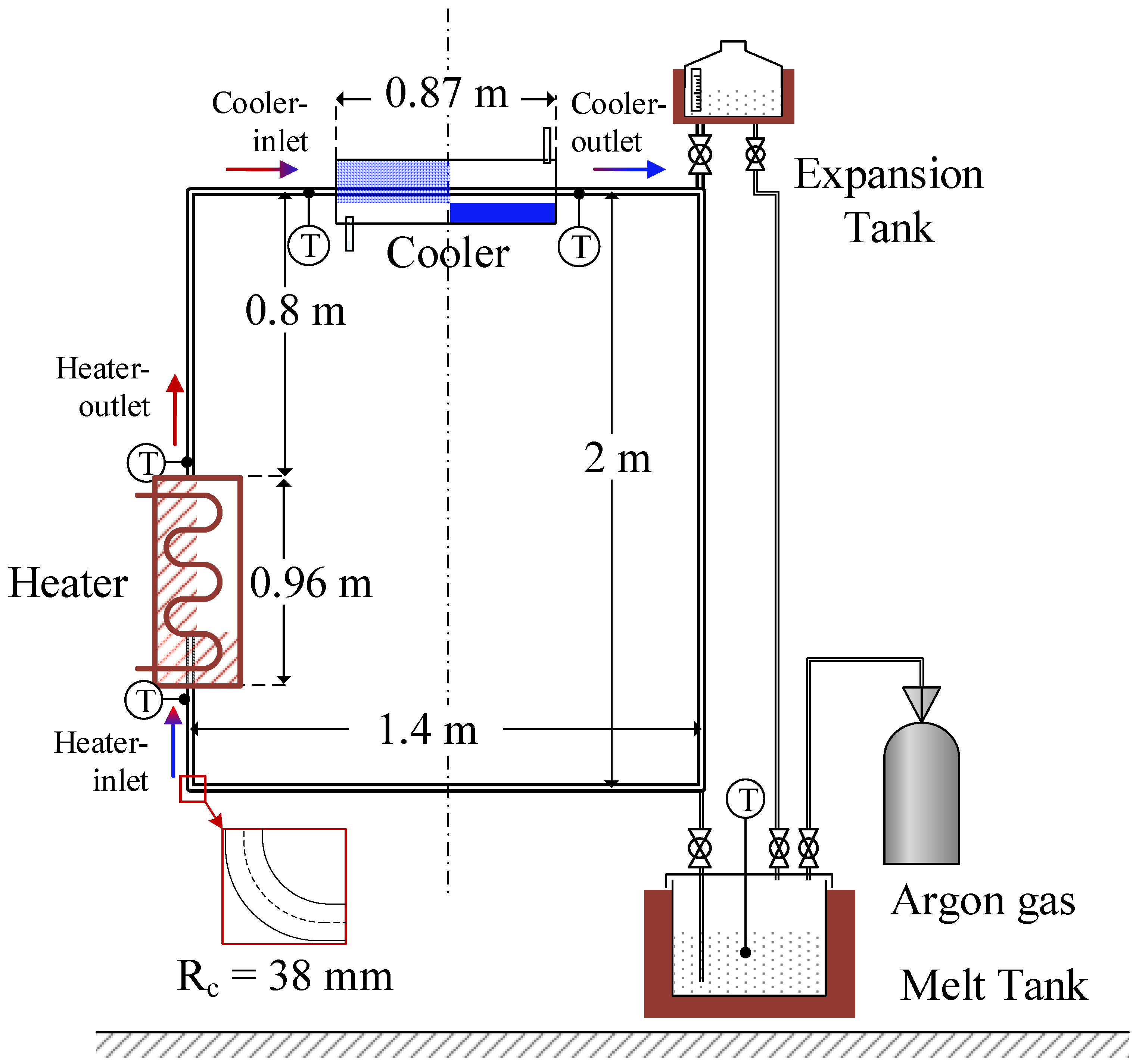
The validation of the present numerical work is carried out against the experimental results of the Molten Salt Natural Circulation Loop (MSNCL), which has been described in detail by Srivastava et al. [25]. A simplified schematic of the facility is shown in Figure 1. The loop is fabricated from Inconel 625 piping and arranged in a rectangular configuration with a height of approximately 2 m and a width of 1.4 m. The pipe used in the experiment follows the ANSI standard designation of 15 mm NB (1/2”) SCH 80. NB refers to the nominal bore size, while the corresponding pipe has an inner diameter of 13.88 mm and a wall thickness of 3.73 mm. Additionally, it has a bending radius of 38 mm following the ANSI standard. The loop is supplied with molten salt that is initially melted in the melt tank and transferred into the main circuit by pressurizing the melt tank with argon gas. Once the loop is charged, natural circulation is established through electrical heating in the heater section and forced air cooling in the cooler section. Although the system operates as a closed loop, the terms inlet and outlet are used in the heater and cooler regions to distinguish the locations where the bulk fluid enters and leaves each section. All inlet and outlet reference points are positioned approximately 10 cm upstream or downstream of the respective component.

The primary driving mechanism is buoyancy, where density differences between the heated and cooled sections induce continuous circulation of the molten salt. Temperature sensors are located at the inlet and outlet of both the heating and cooling sections, providing the bulk temperature data used for validation in this study. As molten salt undergoes thermal expansion and contraction during operation, an expansion tank is integrated at the top of the loop to maintain safe operating pressure and to accommodate volume fluctuations. Although the system can support multiple heater–cooler configurations [21], the present study focuses specifically on the vertical heater–horizontal cooler (VHHC) arrangement adopted in the experimental setup [25]. The design and preparation of the loop, including argon purging, pressurization of the melting tank for initial salt charging, and emptying of the expansion tank, are explained in detail by Srivastava et al. [25]. In the present study, these steps are only summarized and referenced, as the focus remains on the benchmark temperature and velocity data.

3. Numerical Method

3.1. Governing Equation

The molten salt flow is modeled as a single-phase, incompressible fluid with heat transfer, governed by the conservation of mass, momentum, and energy. In natural circulation, buoyancy forces generated by temperature-dependent density variations drive the flow. The Boussinesq approximation is applied, treating density as constant except in the gravity term, where it varies linearly with temperature (Equation (1)). The thermal expansion coefficient (β) represents the rate of density change with temperature relative to a reference state (ρ₀). The unit of the thermal expansion coefficient is [1/K].

$$\beta =-{\displaystyle \frac{1}{{\rho }_0}}{\left({\displaystyle \frac{\partial \rho }{\partial T}}\right)}_{T_0}$$

(1)

The flow field was solved using either a laminar or Transition SST turbulence model to represent momentum transport. Both models assume a single-phase, incompressible, Newtonian fluid. The incompressibility condition is expressed by the continuity equation (Equation (2)), where u and v denote the velocity components in the horizontal (x) and vertical (y) directions, respectively, ensuring mass conservation throughout the domain.

$${\displaystyle \frac{\partial \mathbf{u}}{\partial x}}+{\displaystyle \frac{\partial \mathbf{v}}{\partial y}}=0$$

(2)

The momentum equations for the laminar model are given in Equations (3) and (4) for the x and y directions, respectively. The left-hand side represents unsteady and convective momentum transport, while the right-hand side includes pressure gradient (∂ρ) and viscous diffusion terms arising from the fluid viscosity (μ). In the y-direction momentum equation (Equation (4)), a gravitational body-force term is included to account for natural convection induced by buoyancy. The gravitational acceleration (g) is coupled with the thermal expansion relation defined in Equation (1).

$${\rho }_0\left({\displaystyle \frac{\partial \mathbf{u}}{\partial t}}+\mathbf{u}{\displaystyle \frac{\partial \mathbf{u}}{\partial x}}+\mathbf{v}{\displaystyle \frac{\partial \mathbf{u}}{\partial y}}\right)=-{\displaystyle \frac{\partial p}{\partial x}}+\mu \left({\displaystyle \frac{{\partial }^2\mathbf{u}}{\partial x^2}}+{\displaystyle \frac{{\partial }^2\mathbf{u}}{\partial y^2}}\right)$$

(3)

$${\rho }_0\left({\displaystyle \frac{\partial \mathbf{v}}{\partial t}}+\mathbf{u}{\displaystyle \frac{\partial \mathbf{v}}{\partial x}}+\mathbf{v}{\displaystyle \frac{\partial \mathbf{v}}{\partial y}}\right)=-{\displaystyle \frac{\partial p}{\partial y}}+\mu \left({\displaystyle \frac{{\partial }^2\mathbf{v}}{\partial x^2}}+{\displaystyle \frac{{\partial }^2\mathbf{v}}{\partial y^2}}\right)+{\rho }_0\overrightarrow{g}-{\rho }_0\beta (T-T_0)\overrightarrow{g}$$

(4)

The Transition SST turbulence model combines the k–ω formulation near the wall and the k–ε behavior in the free stream, while incorporating two additional transport equations to predict the onset and length of transition. The model calculates the effective viscosity as

$${\mu }_{eff}=\mu +{\mu }_t$$

(5)

where μ is the dynamic viscosity [Pa·s], and the subscript t represents turbulent eddy viscosity.

The evolution of k and ω follows the SST formulation of Menter [30] and is presented in Equations (6)–(9). In Equations (6) and (7) the term P_k represents the production of turbulent kinetic energy caused by mean velocity gradients, while Y_k denotes the turbulent dissipation rate. The coefficients α, β, σ_k, and σ_ω are empirically calibrated constants that control the relative strength of turbulence production, dissipation, and diffusion in the SST framework. In particular, α governs the coupling between the turbulence production term P_k and the dissipation rate ω determining how rapidly turbulence develops in response to local shear. The coefficient β modulates the destruction rate of ω, thereby influencing the overall level of turbulent viscosity in equilibrium regions. The diffusion coefficients σ_k and σ_ω adjust the rate at which k and ω are transported across the flow domain, balancing the interaction between near-wall and free-stream turbulence. To ensure numerical stability and physical consistency across these regions, the SST model employs blending functions that transition smoothly between the standard k–ω formulation near walls—where it resolves viscous sublayers—and the k–ε type behavior in the free stream ω. This blending approach allows the model to capture wall-bounded shear flows and separation zones more accurately than conventional two-equation models.

$${\displaystyle \frac{\partial (\rho k_{TKE})}{\partial t}}+{\displaystyle \frac{\partial ({\mathbf{u}}_j)}{\partial x_j}}=P_k-Y_k+{\displaystyle \frac{\partial }{\partial x_j}}\left[\left(\mu +{\displaystyle \frac{{\mu }_t}{{\sigma }_k}}\right){\displaystyle \frac{\partial k_{TKE}}{\partial x_j}}\right]$$

(6)

$${\displaystyle \frac{\partial \left(\rho \omega \right)}{\partial t}}+{\displaystyle \frac{\partial \left(\rho {\mathbf{u}}_j\omega \right)}{\partial x_j}}=\alpha {\displaystyle \frac{\omega }{k}}{P}_k-{\beta }_t\rho {\omega }^2+{\displaystyle \frac{\partial }{\partial x_j}}\left[\left(\mu +{\displaystyle \frac{{\mu }_t}{{\sigma }_{\omega }}}\right){\displaystyle \frac{\partial \omega }{\partial x_j}}\right]$$

(7)

To capture laminar–turbulent transition phenomena, two additional transport equations are solved: the intermittency (γ)and the transition momentum thickness Reynolds number (Re_θ) in Equations (8)–(9). The intermittency acts as a blending function between laminar and turbulent regimes, ranging from 0 (fully laminar) to 1 (fully turbulent). Its source term Pγ activates transition onset based on local strain rate and turbulence intensity, while Eγ suppresses premature turbulence production. The momentum thickness Reynolds number (Re_θ) governs the transition onset location, with its transport equation calibrated through the empirical correlations of Langtry and Menter [30]. The term P_Reθ adjusts Re_θ according to local turbulence and pressure-gradient effects, allowing the model to reproduce a wide range of natural and forced transition mechanisms. Through the coupling of γ and Re_θ with the k–ω SST framework, the Transition SST model effectively suppresses turbulence in laminar regions and triggers it when physical instability conditions are met. This approach enables more accurate representation of low-Reynolds-number, buoyancy-driven flows such as natural circulation in molten salts.

$${\displaystyle \frac{\partial \left(\rho \gamma \right)}{\partial t}}+{\displaystyle \frac{\partial \left(\rho u_j\gamma \right)}{\partial x_j}}=P_{\gamma }-E_{\gamma }+{\displaystyle \frac{\partial }{\partial x_j}}\left[\left(\mu +{\displaystyle \frac{{\mu }_t}{{\sigma }_{\gamma }}}\right){\displaystyle \frac{\partial \gamma }{\partial x_j}}\right]$$

(8)

$${\displaystyle \frac{\partial \left(\rho {\mathrm{Re}}_{\theta }\right)}{\partial t}}+{\displaystyle \frac{\partial \left(\rho u_j{\mathrm{Re}}_{\theta }\right)}{\partial x_j}}=P_{{\mathrm{Re}}_{\theta }}+{\displaystyle \frac{\partial }{\partial x_j}}\left[{\sigma }_{\theta }\left(\mu +{\mu }_t\right){\displaystyle \frac{\partial {\mathrm{Re}}_{\theta }}{\partial x_j}}\right]$$

(9)

The energy transport equation governs the temperature field and describes the balance between convective and diffusive heat transfer within the molten salt loop. For laminar flow, it is expressed in Equation (10), where C_p is the specific heat capacity and k is the thermal conductivity. The left-hand side represents the transient and convective transport while the right-hand side represents heat conduction at x- and y-direction. Equation (11) describes the energy equation for turbulent flow, in which the molecular conductivity is replaced by the effective thermal conductivity (k_eff).

The effective conductivity is defined in Equation (12). The term (k_eff) accounts for both molecular conductivity and turbulent heat diffusion, with the latter term enhancing energy transport in regions of high turbulence intensity. The term μ_t is the turbulent eddy viscosity and Pr_t is the turbulent Prandtl number. The turbulent Prandtl number used in this study is 0.85, which is a typical value for liquids. In essence, Equations (10)–(12) capture both the laminar and turbulent heat-transfer mechanisms governing buoyancy-driven natural circulation. While molecular conduction dominates in quiescent regions, the addition of μ_t/Pr_t substantially increases the local thermal diffusivity where turbulence develops, improving the prediction of temperature gradients between the heater and cooler sections of the loop.

$$\rho C_p\left({\displaystyle \frac{\partial T}{\partial t}}+\mathbf{u}{\displaystyle \frac{\partial T}{\partial x}}+\mathbf{v}{\displaystyle \frac{\partial T}{\partial y}}\right)={\displaystyle \frac{\partial }{\partial x}}\left(k_f{\displaystyle \frac{\partial T}{\partial x}}\right)+{\displaystyle \frac{\partial }{\partial y}}\left(k_f{\displaystyle \frac{\partial T}{\partial y}}\right)$$

(10)

$$\rho C_p\left({\displaystyle \frac{\partial T}{\partial t}}+\mathbf{u}{\displaystyle \frac{\partial T}{\partial x}}+\mathbf{v}{\displaystyle \frac{\partial T}{\partial y}}\right)={\displaystyle \frac{\partial }{\partial x}}\left(k_{eff}{\displaystyle \frac{\partial T}{\partial x}}\right)+{\displaystyle \frac{\partial }{\partial y}}\left(k_{eff}{\displaystyle \frac{\partial T}{\partial y}}\right)$$

(11)

$$k_{eff}=k_f+{\displaystyle \frac{{\mu }_t{C}_p}{{\mathrm{Pr}}_t}}$$

(12)

3.2. Geometry and Mesh

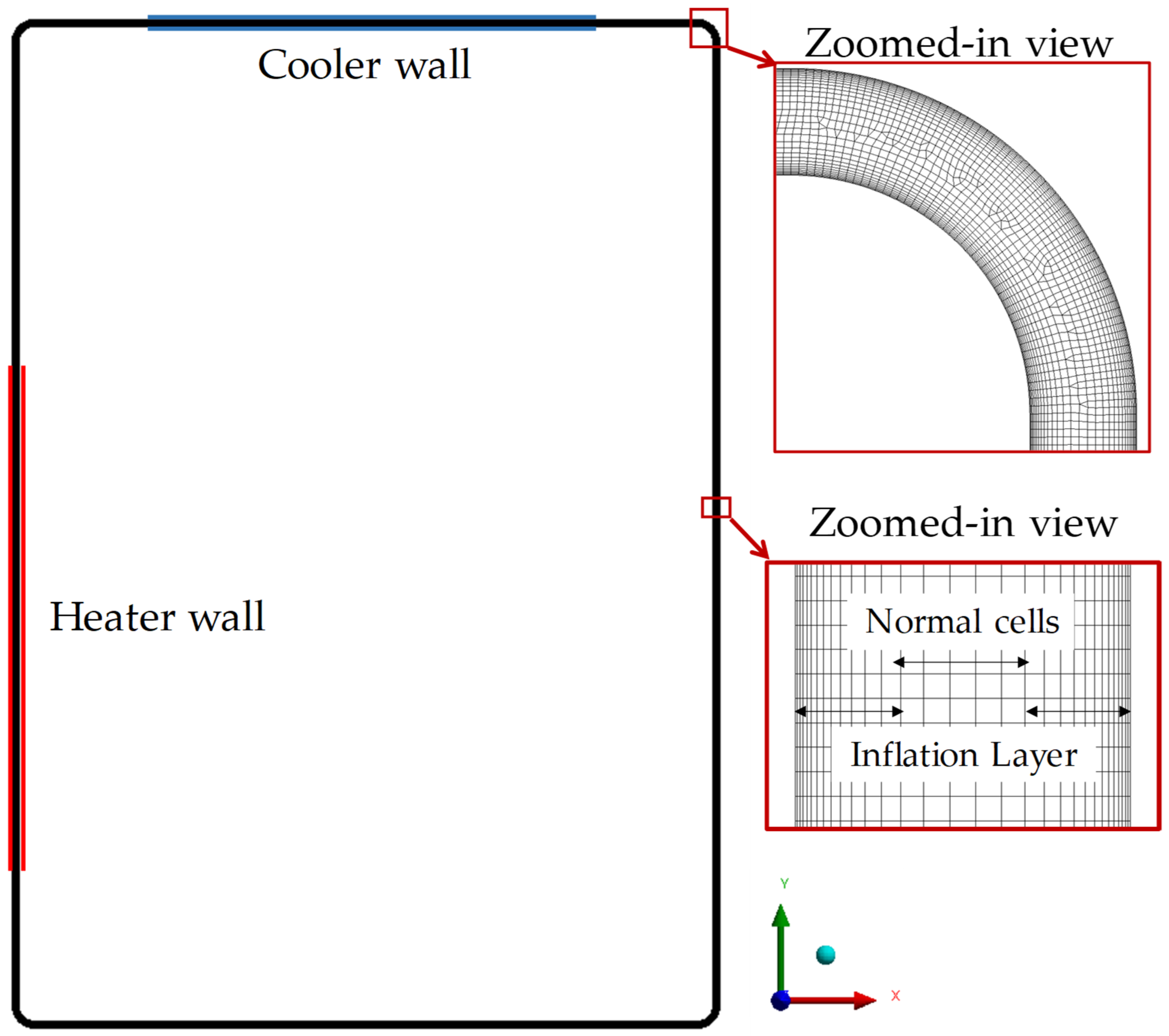
A two-dimensional model of the Molten Salt Natural Circulation Loop (MSNCL) was developed based on the experimental setup of Srivastava et al. [25], which serves as the validation reference. The geometry represents a rounded-rectangle loop comprising vertical riser and downcomer sections connected by horizontal arms and curved bends. As shown in the experimental diagram in Figure 1, the loop height and width are 2000 mm and 1400 mm, respectively, with bends of 38 mm centerline radius following ANSI standards for NPS 1/2” piping. Minor structural details such as fittings and ports were omitted, as they have a negligible influence on the overall flow behavior. This geometric simplification aligns with prior numerical studies aimed at capturing the dominant hydrodynamic characteristics rather than precise construction details.

To ensure mesh quality consistent with established CFD standards, the inflation layer structure and overall grid refinement were redesigned following widely used best-practice guidelines. These include the ERCOFTAC/QNET-CFD Best Practice Guidelines for Industrial CFD [37] and the ANSYS recommendations for the SST and Transition SST turbulence models (minimum BL resolution, smooth layer growth, and y+ ≈ 1) [38]. These guidelines emphasize the need for sufficient boundary layer layers (10–20 layers), controlled growth ratios (1.1 ~ 1.2), and avoidance of abrupt transitions between the boundary-layer mesh and core cells. The summary of mesh settings and statistics is shown in

Table 1. Summary of mesh configuration.

# Mesh	Description	Normal Cell Size [mm]	First Layer Thickness [mm]	Inflation Layer [-]	Inflation Growth [-]	Number of Elements [-]
3	Coarse	1.1	0.12	12	1.2	166,916
2	Medium	1	0.09	14	1.2	206,449
1	Fine	0.8	0.08	16	1.15	314,925

. The mesh structure is visualized in Figure 2 to illustrate the overall arrangement, while the geometrical details can be referred to in Figure 1.

Mesh verification was carried out using three mesh levels: coarse, medium, and fine. The comparison was performed in two ways. First, transient-averaged quantities were evaluated to confirm that the global solution remains independent of mesh resolution over time. Second, local mesh independence was assessed by comparing radial distributions of key parameters obtained from each mesh. All comparisons were quantified using three error metrics—MAE, RMSE, and MAPE—which are described in Section 3.5 (Error Analysis). The detailed results of the mesh-verification study are presented and discussed in Section 4.1 (Mesh Verification)

3.3. Material, Boundary, and Initial Condition

The working fluid is a 60:40 wt% mixture of sodium nitrate (NaNO₃) and potassium nitrate (KNO₃). Its thermophysical properties are treated as temperature-dependent functions based on correlations reported in the literature [39], consistent with earlier 1-D [25] and 3D [27] modeling studies. The polynomial coefficients used to compute these temperature-dependent properties are listed in

Table 2. Polynomial constant for temperature-dependent properties of nitrate salt [23,25,29].

Parameter	a	b	c	d
k [W/m · k]	0.443	1.9 × 10−4	-	-
Cp [J/kg · K]	1443.0	0.172	-	-
μ [mPa · s]	22.714	−0.120	2.281 × 10−4	−1.474 × 10−7

, where the polynomial correlations were derived from temperature–property datasets reported in the literature, with temperature provided in metric units (°C). For density, the Boussinesq approximation is applied, using the density at 200 °C (1950 kg/m³) and a thermal expansion coefficient (β) of 3.26 × 10⁻⁴ [1/K]. In the Boussinesq approximation, density variation is applied only within the buoyancy source term, while the momentum and continuity equations use a constant reference density. In this study, preliminary simulations were performed to estimate the steady-state bulk temperature for each operating condition. The corresponding density at this temperature was then assigned as the operating density for that case. The loop walls are modeled as Inconel 625, matching the experimental setup, and the corresponding solid-material properties of Inconel-625 wall are taken from Ref. [30].

Boundary conditions are specified separately for momentum and energy transport. For momentum, all internal walls are treated as no-slip boundaries, enforcing zero velocity at the solid surfaces. Since the loop is closed, no inlet or outlet conditions are required; circulation develops purely from buoyancy forces. Gravity is applied in the vertical direction with an acceleration of (negative) −9.81 m/s², acting downward. For energy boundary conditions, the molten salt operates between 200 and 500 °C (≈473–773 K), consistent with the benchmark experiment. The heating section is modeled using a uniform heat flux corresponding to 1500–2000 W, while the cooling section is prescribed as an isothermal wall at 200–220 °C (≈473–493 K) to represent forced air cooling.

The heat flux applied at the heating section is defined to represent the heat transfer from the electrical heating wire, through the Inconel-625 wall, and into the molten salt. The imposed heat flux is calculated from the heater power and the outer surface area using q = Q/A. This heat flux is assigned to a wall thickness of 3.73 mm to accurately represent the thermal resistance of the Inconel-625 tube. The detailed heat flux values corresponding to each heater power are summarized in

Table 3. Thermal BCs and wall-resolution indicator.

Heater Power [W]	Heater Heat Flux [W/m2]	Cooling Temperature [C]	Maximum y+
1500	23,306.43	200	0.70
1600	24,860.19	200	0.74
1700	26,413.95	200	0.78
1800	27,967.71	212	0.84
1900	29,521.48	212	0.87
2000	31,075.24	215	0.91

. For the cooling section, an isothermal boundary is applied. The assigned wall temperature is selected based on the minimum cooling-wall temperatures reported in the benchmark experiment, and the values used in this study are listed in Table 3. All remaining loop walls are treated as adiabatic, with zero heat flux.

To verify adequate near-wall resolution for the SST-based turbulence model, the non-dimensional wall distance y+ was evaluated along the wall for all operating powers. Because y+ increases with velocity and therefore varies with heater power, the maximum value at each operating condition is reported in Table 3 as a representative indicator of wall resolution. Across all cases, the maximum y+ remained close to unity (typically ≲ 1) [40], confirming that the viscous sublayer is fully resolved and that the formulation of the Transition SST model is operating within its recommended range.

Due to the transient nature of the simulation and the molten salt being initially stagnant at t = 0, the Transition SST model could not be applied directly. Activating the turbulence and transition transport equations in a zero-velocity field often leads to numerical instability. To prevent this, the flow was first advanced using the laminar model until t = 10 s, allowing buoyancy forces to establish a stable circulation pattern. After this period, the turbulence formulation was switched to the Transition SST (γ–Reθ) model. When the model is activated, the existing velocity and temperature fields are preserved, while the turbulence variables (k, ω, γ, and Reθ) are initialized by ANSYS Fluent 18.0 (release date May 2017) using either its built-in default starting values or the standard near-wall correlations of the Transition SST formulation (

Table 4. Turbulence boundary condition and initialization.

Parameter	Symbol	Wall BC	Description
Turbulent Kinetic Energy	k	Not prescribed	Computed through iteration using Menter’s near-wall correlation [40]
Specific dissipation rate	ω	Not prescribed
Intermittency	γ	0	Enforces laminar wall boundary layer
Transition momentum thickness Reynolds number	Reθ	0	Ensures no imposed transition onset [41]
Interior initial values	k, ω, γ, Reθ	-	k = 1, ω = 1, γ = 1, Reθ = 1 Fluent default initialization [40]

). Initial interior values at Table 4 (row 4) serve only as initial guesses for the first iteration; the γ–Reθ transport equations immediately overwrite them based on the locally developed velocity gradients and temperature distribution. Consequently, the turbulence field observed at t = 10.1 s is generated entirely by the physics of the evolving flow, not by any imposed inlet or wall specification. All remaining constants and auxiliary correlation parameters of the SST and γ–Reθ models were retained exactly as implemented in ANSYS Fluent, following the original Langtry–Menter formulation [40].

3.4. Modeling Approach and Numerical Scheme

The simulations were performed in transient mode using the pressure-based solver in ANSYS Fluent 18.1 [42]. The governing equations are the incompressible Navier–Stokes equations with gravity applied in the vertical direction to represent buoyancy forces. Pressure–velocity coupling is handled with the SIMPLE algorithm, and the transient formulation uses a first-order implicit scheme. The first-order implicit method is unconditionally stable for strongly coupled flow problems [43], which is important in this study because viscosity depends on temperature through a third-order polynomial, creating strong coupling between the momentum and energy equations under buoyancy-driven conditions. Spatial discretization is performed using second-order schemes for both convection and diffusion terms.

Convergence criteria were set to residual tolerances of 10⁻⁴ for continuity and velocity, and 10⁻⁷ for energy. The turbulence transport equations—k, ω, intermittency, and the transition Reynolds number—were maintained at the default Fluent thresholds of 10⁻³. The solver exhibited stable convergence behavior, requiring fewer than 50 iterations per time step during the early transient period. As the system approached a quasi-steady circulation state, where temperature and velocity variations became small, the number of required iterations decreased to 3–4 per time step. This behavior was observed after approximately 1000 s of simulated transient time.

3.5. Error Analysis

Error analysis is applied to quantify the consistency, convergence, and overall validity of the numerical and experimental comparisons in this study. Three widely used norm-based measures are employed: the mean absolute error (MAE), which represents the average magnitude of deviations; the root mean square error (RMSE), which gives greater weight to larger discrepancies; and the mean absolute percentage error (MAPE), which expresses deviations relative to the reference value and is used only when the reference quantity remains sufficiently above zero. These measures are standard in numerical verification and error evaluation [44,45,46] and are defined as follows:

$$MAE={\displaystyle \frac{1}{N}}{\displaystyle \sum _{i=1}^N\left|{\varphi }_i-{\varphi }_i^{ref}\right|}$$

(13)

$$RMSE=\sqrt{{\displaystyle \frac{1}{N}}{\displaystyle \sum _{i=1}^N{\left({\varphi }_i-{\varphi }_i^{ref}\right)}^2}}$$

(14)

$$MAPE={\displaystyle \frac{100}{N}}{\displaystyle \sum _{i=1}^N\left|\frac{{\varphi }_i-{\varphi }_i^{ref}}{{\varphi }_i^{ref}}\right|}$$

(15)

In these expressions, ϕ denotes the evaluated quantity (e.g., velocity, temperature, or eddy viscosity), ϕ ref denotes the chosen reference dataset, and i = 1, …, N indexes, refer to all sampling data. Depending on context, i corresponds either to time instants t_i for transient evaluation or to radial positions r_i sampled at fixed axial stations for spatial (radial) assessment.

4. Results and Discussion

4.1. Mesh Verification

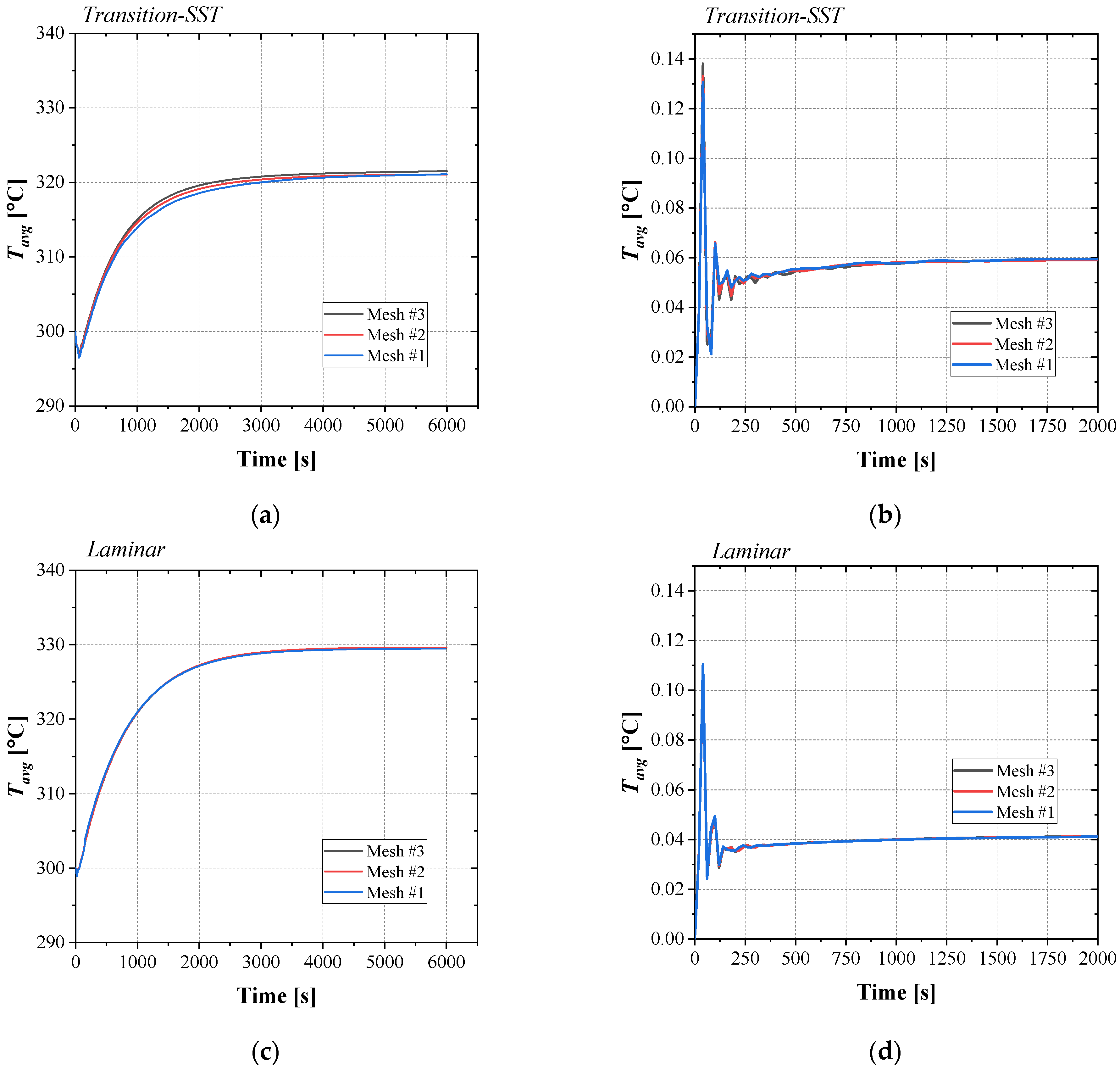
In order to qualitatively assess mesh independence, the system-averaged transient responses—specifically bulk temperature and velocity—were compared across all three mesh levels. System-averaged transient temperature and velocity for the three meshes are presented in Figure 3. These values were obtained by averaging temperature and velocity over the entire domain. For temperature, data were sampled every 20 s up to 6000 s, while for velocity, data were sampled every 20 s up to 2000 s. The shorter time span for velocity is appropriate because the velocity field reaches a steady state much faster than the temperature field.

Across both the Transition SST and laminar models, the transient temperature evolution follows the same overall trend for all mesh levels. The rise toward the quasi-steady state occurs over an identical time scale and with similar curvature, indicating that the transient response is not sensitive to mesh refinement. Although the two models predict different absolute magnitudes—reflecting their different physical formulations—the variation between meshes within each model is minimal. For both models, all three mesh levels collapse onto nearly identical curves, with mesh-to-mesh differences visually indistinguishable throughout the entire transient period. This behavior is consistent in both the bulk temperature response (top panels) and the temperature gradient-derived quantity (bottom panels). The absence of divergence or phase lag between mesh levels confirms that the solution is converged with respect to mesh resolution.

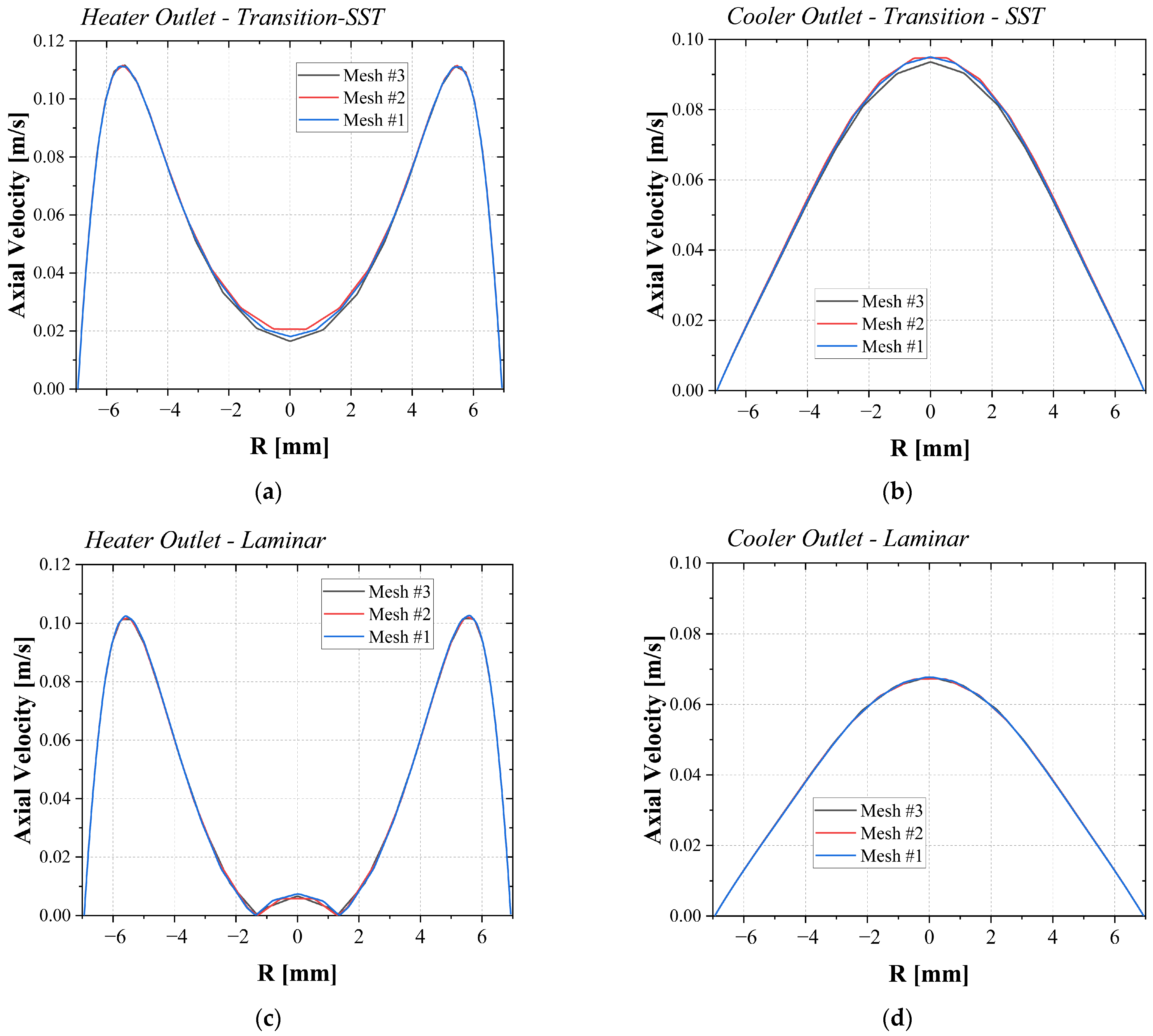
A similar evaluation was performed for the local velocity distributions at the heater and cooler outlets, as shown in Figure 4. The upper panels correspond to the Transition SST predictions, while the lower panels show the Laminar model. On the cooler side, both models produce a smooth, single-peak velocity profile characteristic of a fully developed laminar regime. Turbulence intensity in the Transition SST solution is negligible in this region, and all meshes exhibit nearly identical profile shapes and magnitudes. More pronounced differences appear on the heater side. Both models display the typical M-shaped velocity profile, with near-wall peaks and a central dip caused by strong buoyancy effects adjacent to the heated wall. These features—including peak locations and overall curvature—remain consistent across all mesh levels, indicating robust mesh convergence despite the presence of strong gradients. In the Laminar model, however, the center region shows a sharper velocity reduction, forming a small stagnant-core zone. This behavior is consistent with the observations of Reis et al. [24], who reported that the heater section of natural circulation loops exhibits thermally developing, buoyancy-dominated flow. Under such conditions, intense wall heating accelerates near-wall fluid while the core remains weakly mixed, promoting behaviors that a purely laminar model cannot accurately represent. This explains the magnitude differences between the two models on the heater side, while mesh-to-mesh consistency remains strong. Overall, both the global and local comparisons confirm that the numerical solutions are not sensitive to mesh refinement and that the remaining discrepancies between models originate from physical model differences rather than discretization effects.

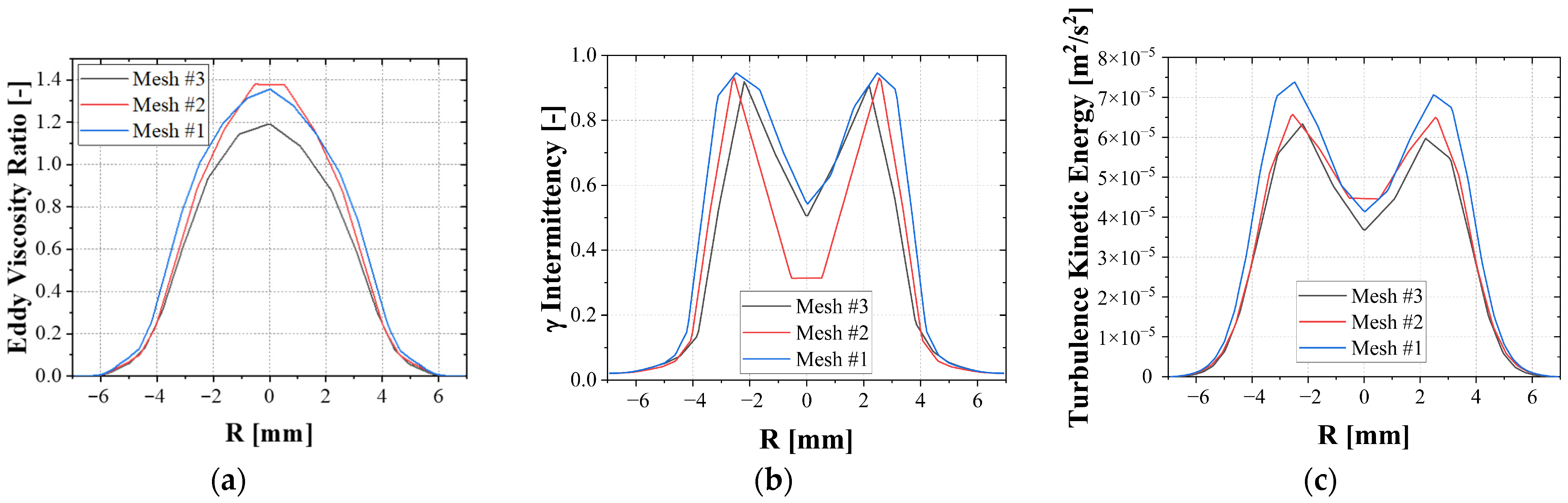
In Figure 5, the turbulence transport quantities—intermittency (γ), eddy viscosity ratio, and turbulence kinetic energy—exhibit greater variation across the mesh levels than the velocity and temperature fields. This behavior is expected because turbulence variables depend directly on local production, dissipation, and wall-gradient processes, which makes them inherently more sensitive to grid resolution. Prior studies have reported that, due to the strong coupling between turbulence and the mean flow, turbulence-field predictions generally show higher mesh sensitivity compared with mean-flow variables [37]. Consequently, even when velocities and temperatures display clear mesh independence, variations in the turbulence transport quantities do not imply a loss of solution accuracy. In the present work, although the magnitudes of γ, eddy viscosity, and TKE differ slightly among meshes, the qualitative features—including profile shapes, peak locations, and the extent of the transition region—remain consistent. This indicates that the Transition SST model maintains a stable and physically coherent representation of the transition process despite the slightly larger discrepancy across meshes.

For quantitative analysis of the sensitivity of the numerical solution to mesh resolution, a systematic mesh-independence assessment was performed for both the Laminar and Transition SST models. Two categories of quantities were examined: system-averaged values and local radial distributions. System-averaged quantities, denoted with the subscript “avg”, were obtained from 300 temporal samples recorded every 20 s throughout the 6000 s transient simulation. Local quantities were evaluated at the heater-outlet (HO) and cooler-outlet (CO) cross-sections, where the entire diameter was interpolated onto 200 uniformly spaced radial points for comparison. Mesh-to-mesh deviations were quantified using three standard error metrics—MAE, RMSE, and MAPE. Here, ε₃₋₂ denotes the error between the coarse and medium meshes, using the medium mesh as the reference, while ε₂₋₁ represents the error between the medium and fine meshes, with the fine mesh serving as the reference. These metrics collectively indicate the extent to which the numerical solution approaches mesh-independent behavior.

Mesh-independence characteristics for both the laminar and Transition SST models are summarized in

Table 5. Quantitative summary of mesh sensitivity study.

Model	Φ	Unit	ε3−2			ε2−1
			MAE	RMSE	MAPE	MAE	RMSE	MAPE
Laminar	Tavg	°C	0.04	0.04	0.01%	0.03	0.2	0.005%
Laminar	uavg	${\displaystyle \raisebox{1ex}{$\mathrm{m}$}\!\left/ \!\raisebox{-1ex}{$\mathrm{s}$}\right.}$	4.6 × 10−5	1.1 × 10−4	0.10%	4.2 × 10−5	2.2 × 10−4	0.11%
Laminar	uHO(R)	${\displaystyle \raisebox{1ex}{$\mathrm{m}$}\!\left/ \!\raisebox{-1ex}{$\mathrm{s}$}\right.}$	1.8 × 10−5	4.9 × 10−4	3.97%	1.3 × 10−4	5.9 × 10−4	2.80%
Laminar	uCO(R)	${\displaystyle \raisebox{1ex}{$\mathrm{m}$}\!\left/ \!\raisebox{-1ex}{$\mathrm{s}$}\right.}$	4.1 × 10−2	3.3 × 10−2	0.001%	5.3 × 10−5	1.4 × 10−4	0.18%
Transition SST	Tavg	°C	0.38	0.32	0.006%	0.45	0.39	0.07%
Transition SST	uavg	${\displaystyle \raisebox{1ex}{$\mathrm{m}$}\!\left/ \!\raisebox{-1ex}{$\mathrm{s}$}\right.}$	3.6 × 10−4	6.6 × 10−4	0.65%	3.6 × 10−4	6.6 × 10−4	0.69%
Transition SST	uHO(R)	${\displaystyle \raisebox{1ex}{$\mathrm{m}$}\!\left/ \!\raisebox{-1ex}{$\mathrm{s}$}\right.}$	1.2 × 10−3	1.7 × 10−3	4.21%	6.0 × 10−4	9.0 × 10−4	2.34%
Transition SST	uCO(R)	${\displaystyle \raisebox{1ex}{$\mathrm{m}$}\!\left/ \!\raisebox{-1ex}{$\mathrm{s}$}\right.}$	1.2 × 10−3	1.4 × 10−3	1.96%	4.0 × 10−4	4.5 × 10−4	0.84%
Transition SST	μt/μavg	$-$	2.0 × 10−3	1.2 × 10−2	0.82%	9.0 × 10−3	9.9 × 10−3	4.39%
Transition SST	γavg	$-$	3.5 × 10−3	8.6 × 10−3	3.07%	5.4 × 10−3	5.6 × 10−3	5.58%
Transition SST	kavg	${\displaystyle \raisebox{1ex}{${\mathrm{m}}^2$}\!\left/ \!\raisebox{-1ex}{${\mathrm{s}}^2$}\right.}$	8.2 × 10−9	5.4 × 10−7	0.67%	2.4 × 10−7	2.6 × 10−7	4.35%
Transition SST	(μt/μ)(R)	$-$	6.9 × 10−2	0.1	12.9%	2.9 × 10−2	5.6 × 10−2	8.27%
Transition SST	γHO(R)	$-$	3.4 × 10−2	0.13	13.5%	0.11	0.15	21.9%
Transition SST	kHO(R)	${\displaystyle \raisebox{1ex}{${\mathrm{m}}^2$}\!\left/ \!\raisebox{-1ex}{${\mathrm{s}}^2$}\right.}$	2.3 × 10−6	3.1 × 10−6	12.9%	3.8 × 10−6	5.8 × 10−6	10.5%

. For the laminar case, the system-averaged temperature and velocity exhibit only very small differences across the three meshes, with MAPE values remaining below approximately 0.2%. The local radial profiles at the heater-outlet cross-section also show excellent agreement, as the profile shapes, peak locations, and overall distributions of velocity and temperature are nearly identical for all mesh levels. These results demonstrate that the laminar solution is effectively mesh-independent, both for system-averaged quantities and for local flow structure.

For the Transition SST model, the system-averaged temperature and velocity also show strong mesh convergence, with sub-percent differences between the medium and fine meshes and only small deviations in the coarse mesh. The local radial profiles of velocity and temperature are likewise consistent across meshes, with only minor variations near the shear-layer region. In contrast, the turbulence-related quantities—intermittency, turbulent kinetic energy, and eddy viscosity ratio—exhibit greater sensitivity to mesh refinement. Their MAPE values typically fall in the 10–15% range for coarse-to-medium comparisons and decrease further when comparing medium to fine meshes. These differences arise mainly in peak magnitude, while all meshes reproduce the same spatial structure, including elevated γ and k near the shear layers and a centerline maximum in the viscosity ratio. This indicates that although turbulence quantities are more mesh-sensitive, the underlying transition pattern remains consistent across all mesh levels. Overall, the medium mesh captures the essential global behavior and local flow structure with sufficient fidelity and is therefore adopted for subsequent analysis.

The overall verification results indicate that the numerical solutions are stable with respect to mesh refinement, and that the medium mesh provides a suitable balance between accuracy and computational cost. In addition, using a refinement ratio of 1.25, the Grid Convergence Index (GCI) suggests that the solution change between M1, M2, and M3 is sufficiently small to fall within the commonly accepted 95% confidence band for grid-verification studies [47,48]. As verification addresses only numerical consistency by quantifying discretization-related uncertainties [47], the following sections focus on validation against experimental data to assess the physical accuracy of the model and its ability to reproduce the observed thermo-hydraulic behavior of the natural circulation system.

4.2. Steady-State and Transient Modeling

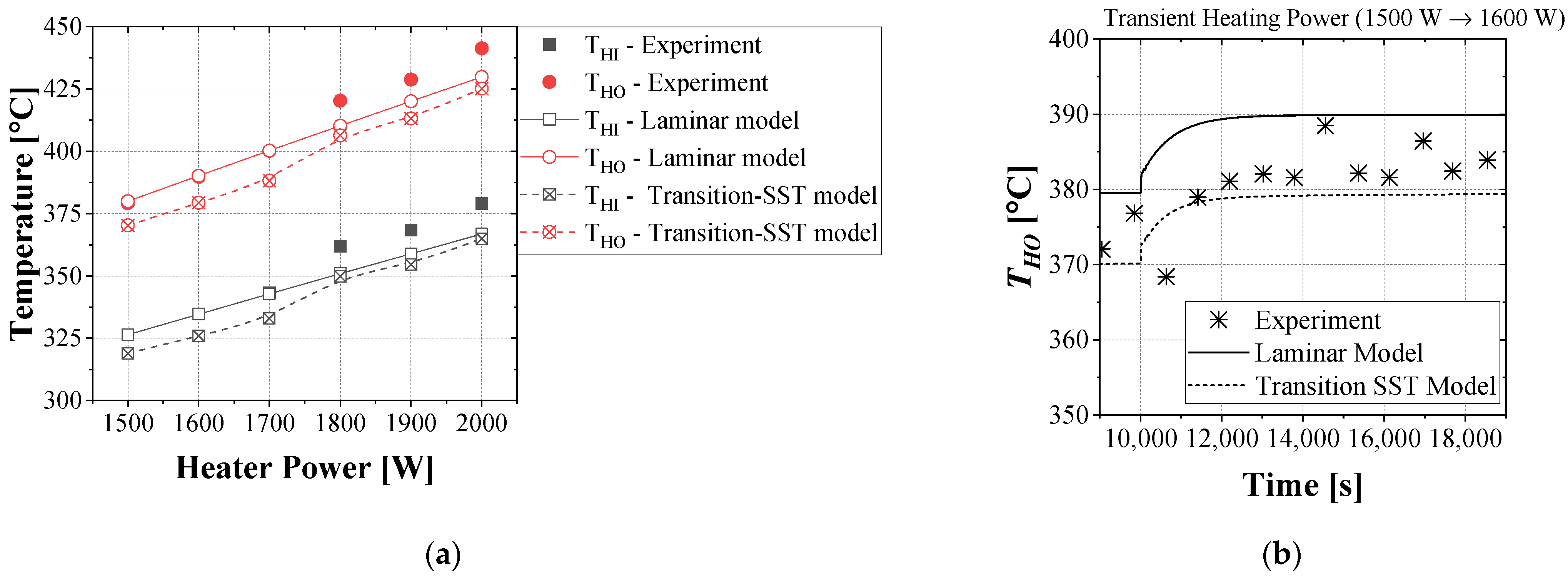
Figure 6a compares the heater-outlet (T_HO) and heater-inlet (T_HI) temperatures between the experimental measurements and the CFD predictions under steady-state conditions. Both the laminar and Transition SST simulations reproduce the experimental temperature trends with only minor deviations, indicating that the model accurately captures the heat-transfer behavior and circulation characteristics of the loop. The predicted temperature range also falls within the stable operating regime of nitrate salt natural circulation systems reported in Refs. [25,27]. The steady-state values were extracted after the loop reached dynamic equilibrium, confirmed by the stabilization of both the heater temperature and the loop-averaged fluid temperature. A quantitative summary of the comparison is provided in

Table 6. Summary of CFD model prediction and experimental comparison for steady-state.

Model	Φ	MAE	RMSE	MAPE
Laminar	THI	9.52 °C	10.82 °C	2.9%
Laminar	THO	6.50 °C	7.50 °C	1.6%
Transition SST	THI	6.44 °C	7.52 °C	1.9%
Transition SST	THO	6.37 °C	7.85 °C	1.5%

.

Figure 6b compares the transient temperature response of the loop between the experimental measurements and the CFD predictions using the laminar and Transition SST models. The simulation was performed under a stepwise heating input: the loop was first operated at 1500 W for 10,000 s to ensure steady-state convergence, after which the heater power was increased to 1600 W for an additional 10,000 s. This procedure enables evaluation of how the system temperature evolves as it transitions toward a new equilibrium condition. Both models successfully reproduce the experimentally observed temperature rise, capturing the gradual thermal response of the molten nitrate salt as circulation strengthens under the increased power. The predicted outlet temperature (THO) increases smoothly and stabilizes after roughly 3000–4000 s, indicating that the simulation accurately represents transient heat accumulation and buoyancy-driven circulation. The Transition SST model responds slightly faster in the early phase and remains closer to the experimental values, though the overall deviation between the two models remains within approximately 5%, which is within the expected experimental uncertainty. These results indicate that, under the present conditions, both models provide physically consistent predictions, confirming that the numerical framework reliably captures the transient thermal behavior of the natural circulation loop.

4.3. Reynolds Number and Velocity Validation

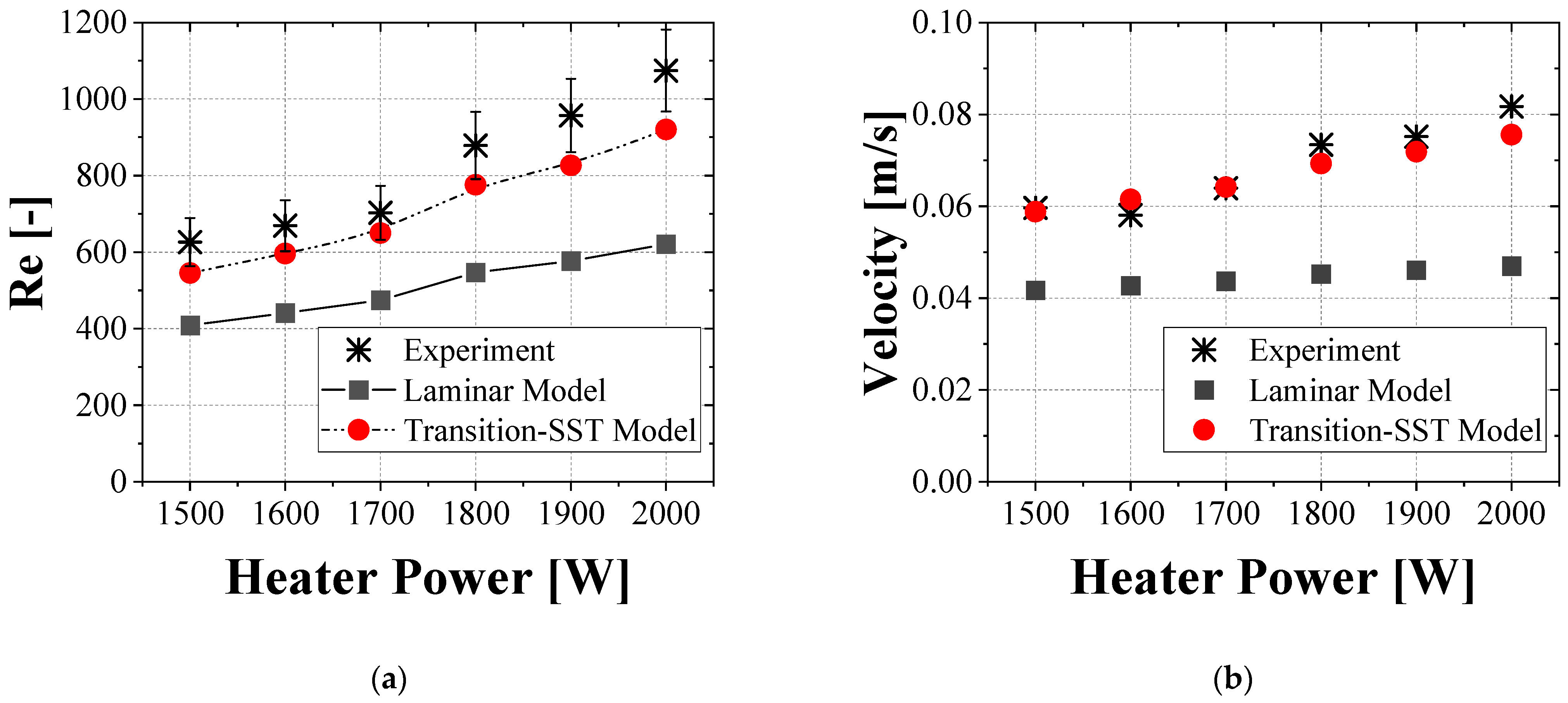
To characterize the circulation strength, both the loop velocity and the corresponding Reynolds number are evaluated. The Reynolds number is computed using Equation (16), where u_avg denotes the system-average velocity, D is the pipe diameter taken as the hydraulic length scale, and the density and viscosity are evaluated at the local operating temperature. Figure 7 shows the variation in Reynolds number and velocity with heater power, comparing CFD predictions against the experimental data. The experimental Reynolds number increases steadily with power, reflecting stronger buoyancy-driven flow as thermal input rises. Both CFD models reproduce this increasing trend, although with different levels of accuracy.

$$\mathrm{Re}={\displaystyle \frac{\rho u_{avg}D}{\mu }}$$

(16)

The laminar model systematically underpredicts the Reynolds number across the entire power range, falling outside the 10% experimental uncertainty band. This underestimation results from the absence of turbulence-related momentum transport, which in reality enhances mixing and supports higher bulk velocities in buoyancy-driven loops. In contrast, the Transition SST model shows much closer agreement with the experimental data, with deviations generally remaining within the ~10% error range. This improved performance demonstrates the model’s capability to represent the mixed-regime flow dynamics characteristic of molten salt natural circulation. A quantitative summary of the error analysis is provided in

Table 7. Summary of error analysis for Reynolds number and velocity prediction.

Model	Φ	MAE	RMSE	MAPE
Laminar	uavg	0.024 m/s	0.025 m/s	34.6%
Laminar	Re	306 [−]	319 [−]	36.8%
Transition SST	uavg	0.003 m/s	0.003 m/s	4.2%
Transition SST	Re	98 [−]	104 [−]	11.8%

.

The difference between the two models can be understood by examining how each interprets the local flow dynamics within the loop. Although the global circulation is driven by the temperature difference between the heating and cooling sections, additional temperature gradients develop locally along the loop walls. These local variations modify buoyancy and viscosity, thereby influencing the detailed velocity distribution. Reis et al. [24] reported that molten salts exhibit near-wall velocity peaks in heated sections due to their high Prandtl number, which causes a thermally underdeveloped boundary layer. In regions with strong vertical temperature gradients—particularly along the vertical legs—this underdeveloped state alters the near-wall acceleration and produces wall-peaked profiles that the laminar model interprets as stagnant-core behavior. The Transition SST model, however, accounts for shear-dependent transport and therefore captures these features more accurately.

4.4. Assessment of Property Variation and Buoyancy Modeling Assumptions

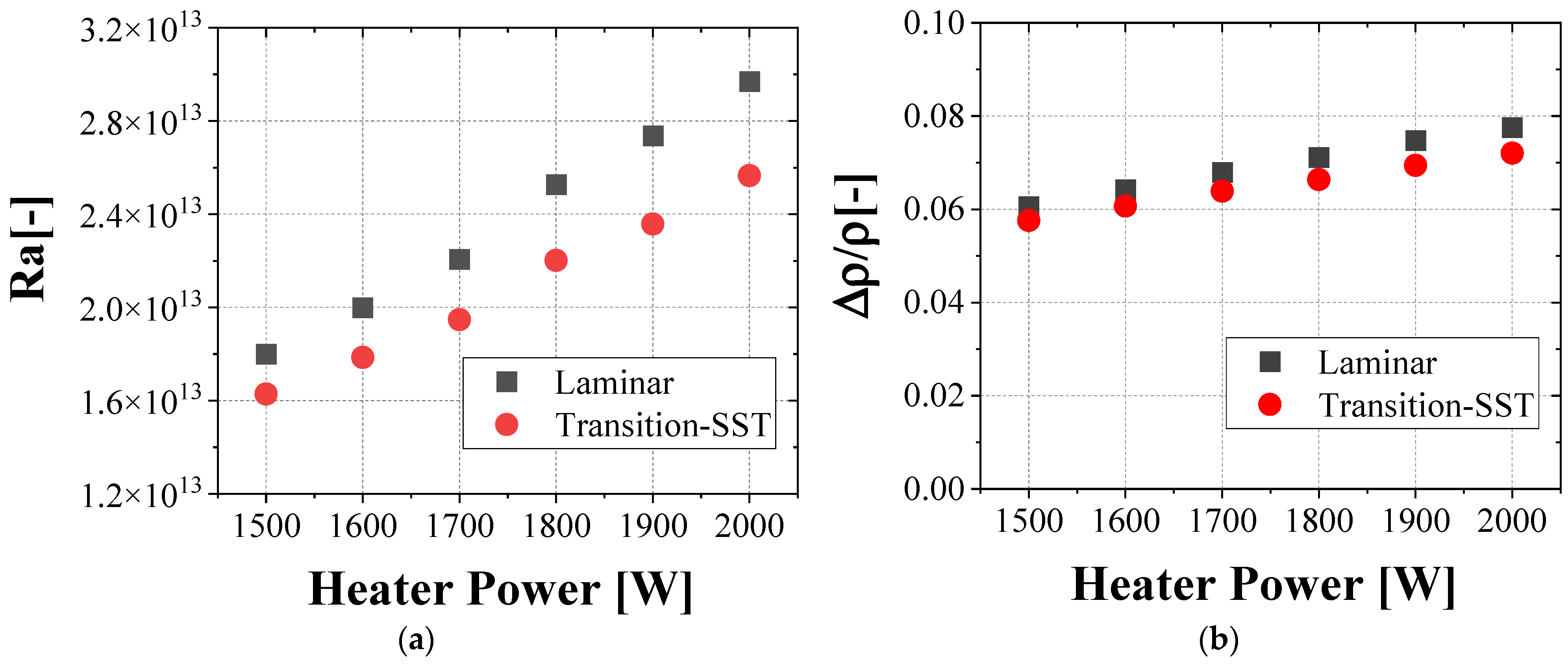
Figure 8 presents the density variation and the corresponding Rayleigh numbers across the simulated heater-power range. The density difference is expressed using the nondimensional ratio Δρ/ρ, where Δρ is computed from the densities evaluated at the maximum and minimum temperatures in the loop. While denominator ρ denotes the operating density. The Rayleigh number is evaluated using Equation (17), with L denoting the buoyancy characteristic length. For Figure 8a (left), L is taken as the full vertical height of the loop (2 m), representing the elevation across which the temperature difference develops and buoyancy acts. This choice also provides a conservative estimate by considering the maximum effective driving length.

$$\mathrm{Ra}={\displaystyle \frac{L^3{\rho }^{2}g\beta \Delta T{C}_p}{\mu k}}$$

(17)

Previous studies, including Kizildag et al. [49] and Gray & Giorgini [50], indicate that density/variation ratios below approximately 0.1 fall within the acceptable range for applying the Boussinesq approximation. Weiss et al. [51] further showed that density variations in the range 0.05–0.1 can remain compatible with stable buoyancy-driven flow at high Rayleigh numbers. The Rayleigh numbers obtained in this work fall well below the upper limits identified in these studies, confirming that the present simulations lie within the regime where the Boussinesq approximation remains valid.

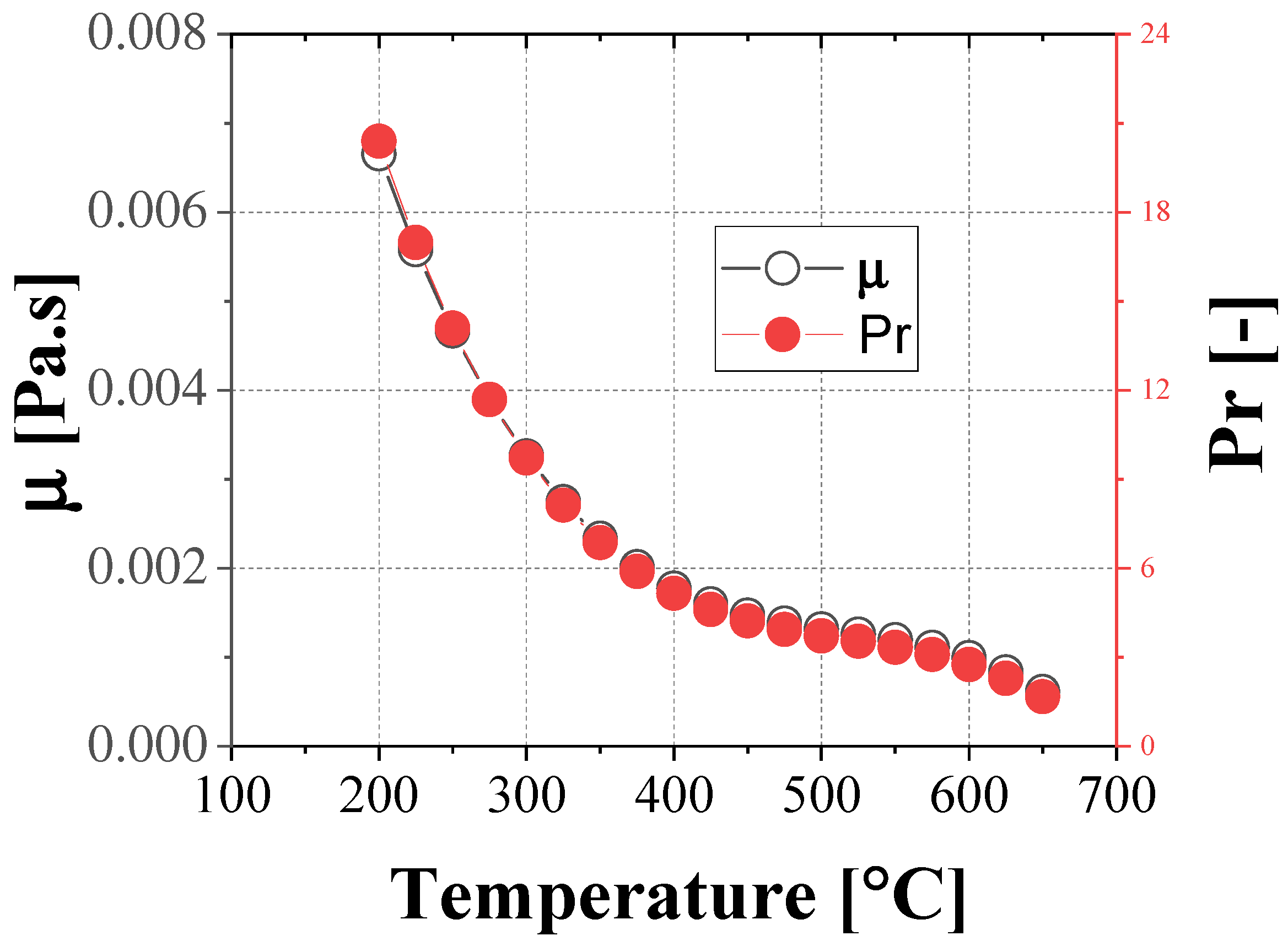
Figure 9 shows the temperature dependence of the dynamic viscosity and Prandtl number of Solar Salt over the operating range. Both quantities decrease strongly with temperature: the viscosity drops by nearly an order of magnitude, and the Prandtl number decreases from values above ~18 to below ~3 at the highest temperatures. This strong variation implies that even modest differences in predicted temperature between the simulations and the experiment can produce noticeable changes in viscosity, and therefore in the Reynolds number. As a consequence, the simulated velocities may agree closely with experimental data while the associated Reynolds numbers exhibit larger discrepancies. In other words, the Reynolds number is highly sensitive to the temperature-dependent viscosity used in its evaluation, whereas velocity remains a more direct and robust metric for comparing CFD predictions with measurements under these conditions.

4.5. Global Parameters and Flow-Regime Characterization

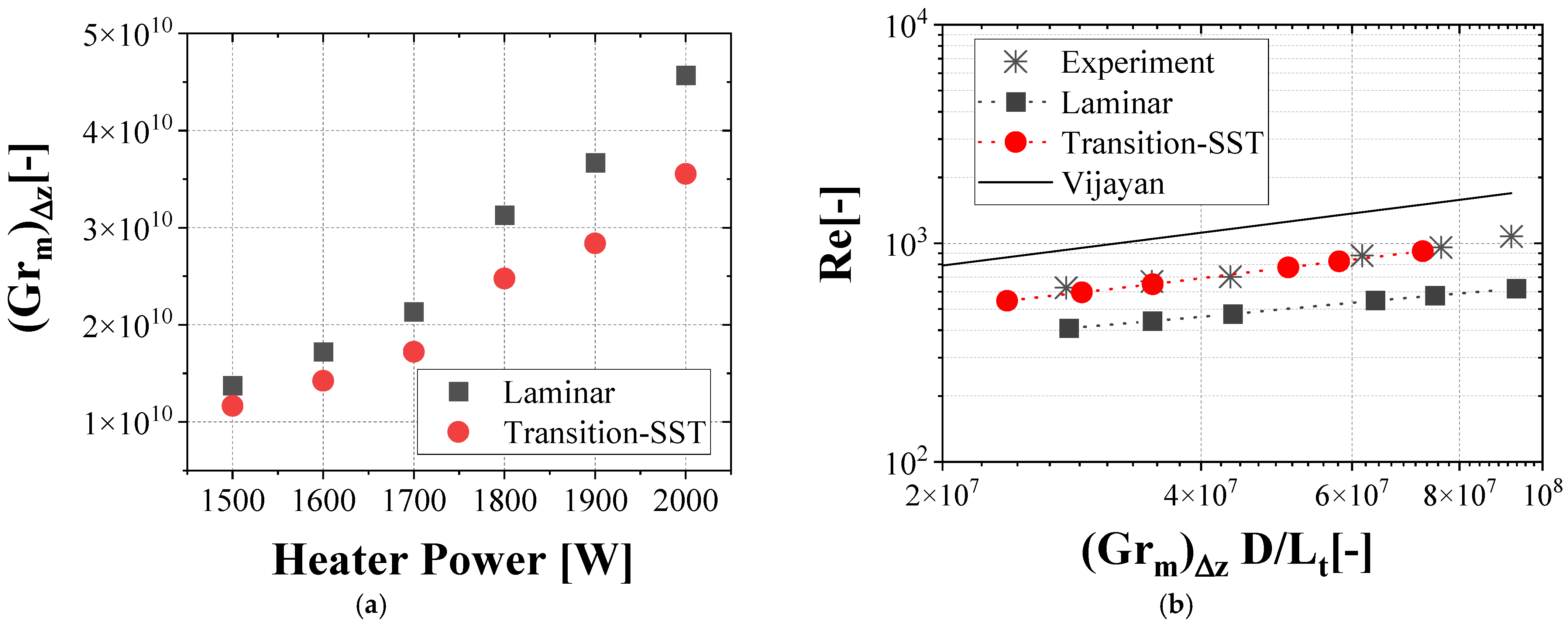
To characterize the overall circulation behavior of the loop, global nondimensional parameters are examined. Figure 10a summarizes the flow regime using the modified Grashof number (Grm)Δz and the corresponding steady-state Reynolds number correlation. The modified Grashof number follows the definition proposed in the benchmark experimental studies and is derived from the classical Grashof number, which represents the ratio of buoyancy to viscous forces. In the formulation introduced by Vijayan et al. [52], the pipe diameter D replaces the characteristic length L, and the temperature difference is replaced by the applied heater power. This modification provides a more practical correlation for natural circulation loops, where heater power is a directly controlled operating variable. As shown in Figure 10, this approach enables a clear relationship among Reynolds number, modified Grashof number, and heater power. The corresponding Gr–Re correlation used for experimental comparison, originally proposed by Vijayan et al. [50], is expressed in Equation (19).

$${\left({\mathrm{Gr}}_{\mathrm{m}}\right)}_{\Delta \mathrm{z}}={\displaystyle \frac{{\mathrm{D}}^3{\rho }^2 \beta \mathrm{g} \mathrm{Q} \Delta \mathrm{z}}{{\mathrm{A} \mu }^3{\mathrm{C}}_{\mathrm{p}}}}$$

(18)

$$\mathrm{Re}=0.1768\left[{\left(G{r}_m\right)}_{\Delta z}{\displaystyle \frac{D}{L_t}}\right]$$

(19)

Figure 10b demonstrates the accuracy of three different approaches. Laminar 2D modeling, 2D Transition SST modeling, and empirical correlation [52]. The empirical correlation tends to over-predict Re relative to the measurements over the present operating range. The Transition SST model yields Reynolds numbers in much closer agreement with the experiment, lying between the laminar prediction and the empirical correlation. However, its (Grm)Δz values are slightly lower than the experimental points. The quantitative comparison is summarized in

Table 8. Summary of MAPE-based error analysis for Reynolds number prediction using three different approaches.

Model	Φ	MAPE
Laminar	Re	34.6%
Transition SST	Re	11.8%
Correlation [52]	Re	58%

, which reports the MAPE values for Reynolds-number prediction obtained from the experimental data, the laminar model, and the Transition SST model. This close agreement of the global parameters (Grm)Δz and velocity suggests that, although the cooler-side boundary condition is simplified as a fixed-temperature (Dirichlet) condition and cannot reproduce the local temperature gradient along the cooler length, its influence on the overall circulation behavior is negligible.

4.6. Local Flow Regime and Profile Development

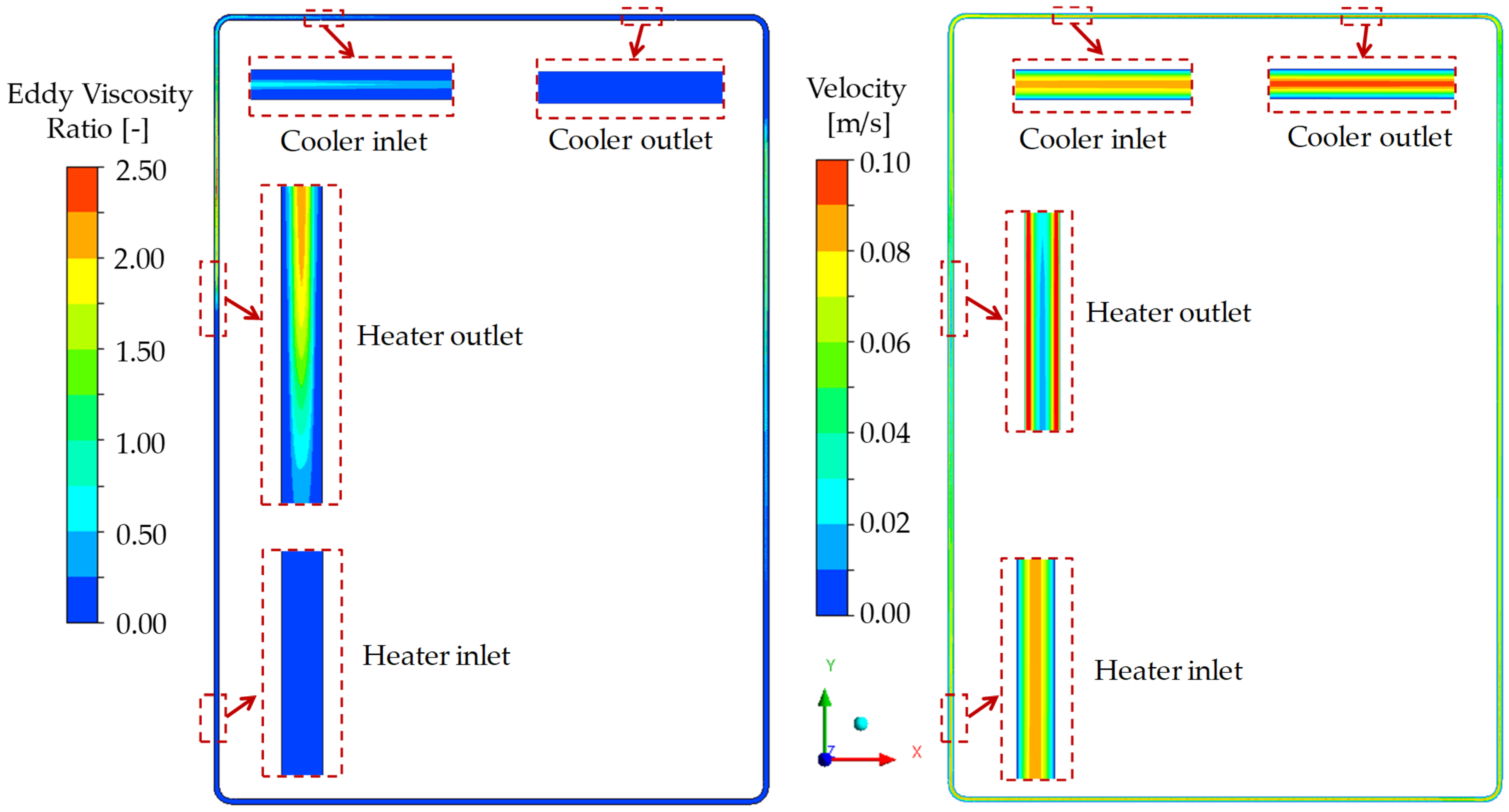
Figure 11 shows that the eddy viscosity predicted by the Transition SST model is concentrated primarily in the vertical legs of the loop, where buoyancy acts in the same direction as the mean flow. In the heated left leg, the strong wall-normal temperature gradient causes the fluid adjacent to the hot wall to become lighter and accelerate upward, while the cooler and denser core fluid rises more slowly. This differential acceleration creates a strongly developing velocity field that the laminar model cannot represent, leading the Transition SST model to generate finite eddy viscosity. As the fluid enters the horizontal cooler section, the bulk flow becomes perpendicular to gravity; buoyancy no longer contributes to the streamwise momentum, the velocity field stabilizes, and the eddy viscosity gradually diminishes. A weaker eddy viscosity layer reappears in the right vertical leg because the incoming fluid remains thermally stratified after passing through the cooler region. When this stratified fluid turns upward, buoyancy again aligns with the flow, causing the denser near-wall fluid to accelerate relative to the warmer core. This effect weakens with height as the temperature field becomes more uniform, resulting in an essentially laminar lower section on the right side. Overall, the spatial pattern of eddy viscosity in Figure 11 reflects how the combined orientation of buoyancy and thermal gradients governs the degree of flow development throughout the loop.

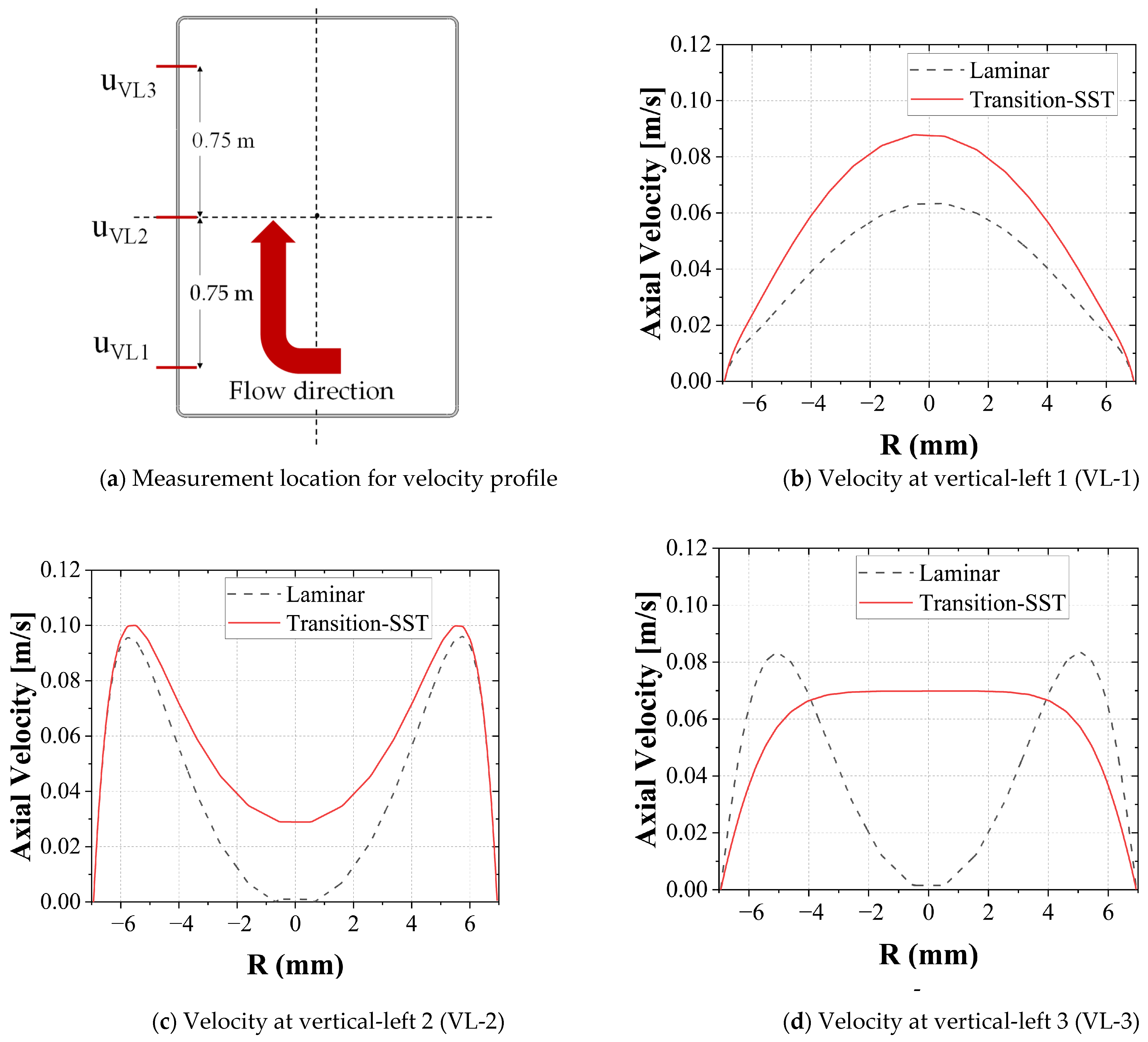
Figure 12 compares the axial-velocity distributions at three vertical locations along the heated leg of the loop: 0.75 m below the mid-height (bottom), near the heater-outlet section (middle), and 0.75 m above the mid-height (top). At the bottom location, where the fluid first enters the heated vertical leg, both models show a developing velocity profile. The Transition SST model predicts slightly stronger near-wall acceleration, whereas the laminar model is more diffusive and exhibits a smoother curvature. At the middle location—where the temperature gradient is strongest—the Transition SST model produces a distinct M-shaped profile with elevated near-wall velocities, while the laminar solution remains more diffused and shows a mild centerline dip characteristic of an under-developed flow. At the top location, as the fluid exits the heated section and approaches the cooler region, the Transition SST model transitions toward a more uniform profile, whereas the laminar model develops more slowly and retains a weak M-shaped curvature. Overall, the Transition SST model captures sharper near-wall gradients and a more realistic development of the velocity profile, while the laminar model remains comparatively diffusive throughout the vertical leg.

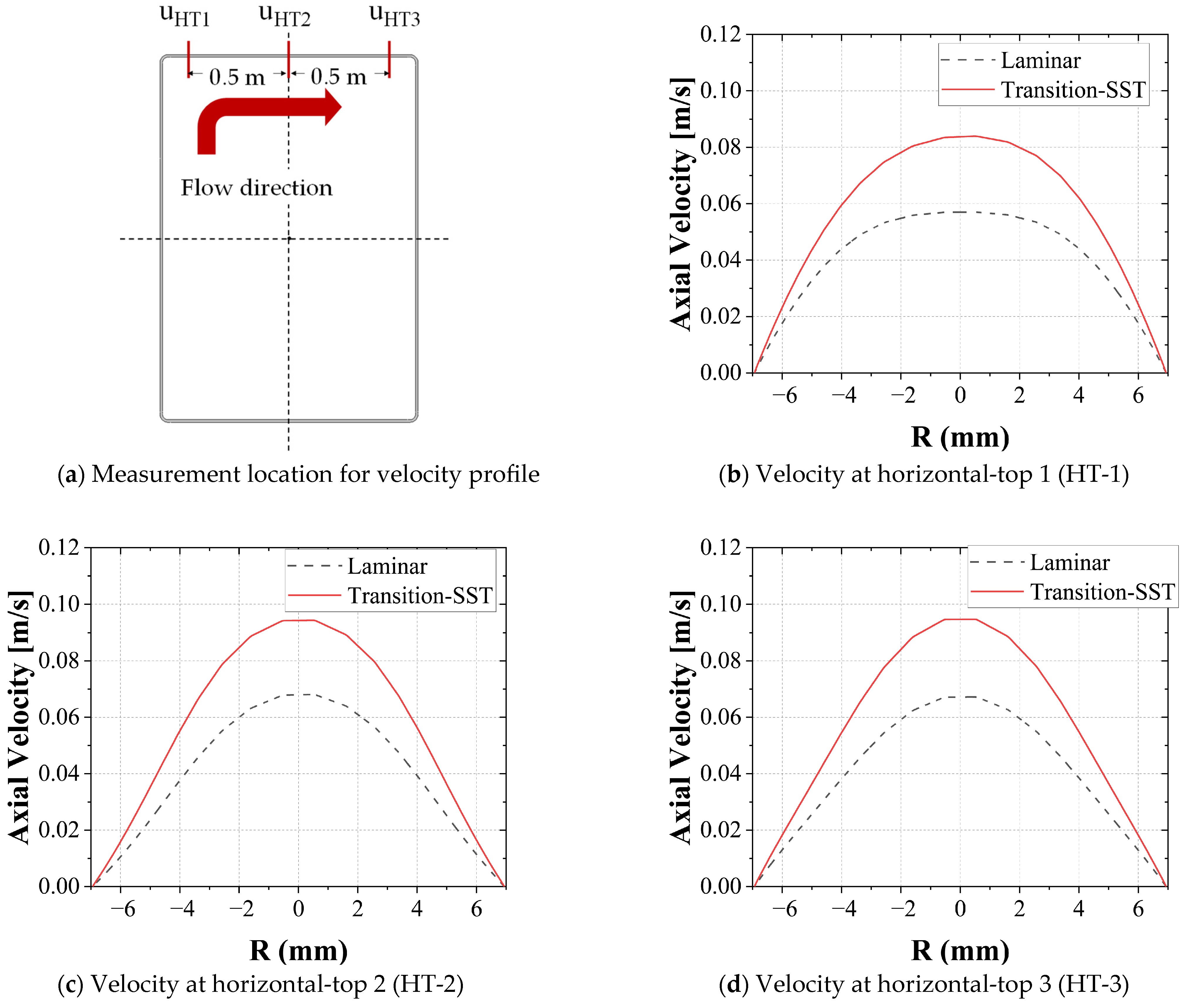
Figure 13 presents the axial-velocity distributions at three locations along the horizontal top leg in the cooler region, spaced 0.5 m apart from left to right. At the left position, where the fluid first enters the horizontal leg, the flow remains in an early developing stage. The laminar model predicts a relatively flat core velocity profile due to its diffusive character, whereas the Transition SST model produces a slightly sharper curvature and a higher centerline velocity, even though turbulence levels in this section remain low. This difference arises because the Transition SST model applies a small shear-based correction to the effective viscosity, which reduces numerical diffusion and allows a more distinct velocity peak to emerge. Further downstream, at the middle and right positions, the velocity profiles progressively approach those expected for a fully developed laminar flow. In these regions, both models yield similar overall shapes, although the Transition SST solution continues to show marginally higher peak velocities and more pronounced near-wall gradients, while the laminar model diffuses the curvature more strongly. Despite the presence of a vertical temperature gradient along the cooled upper wall, no M-shaped structure develops in the horizontal leg profiles. This is because buoyancy acts predominantly in the vertical direction while the main flow proceeds horizontally, limiting its influence on axial momentum. Overall, the horizontal cooler leg exhibits only modest differences between the two models: The Transition SST formulation provides a slightly sharper representation of the developing flow, while both models converge toward similar behavior farther downstream.

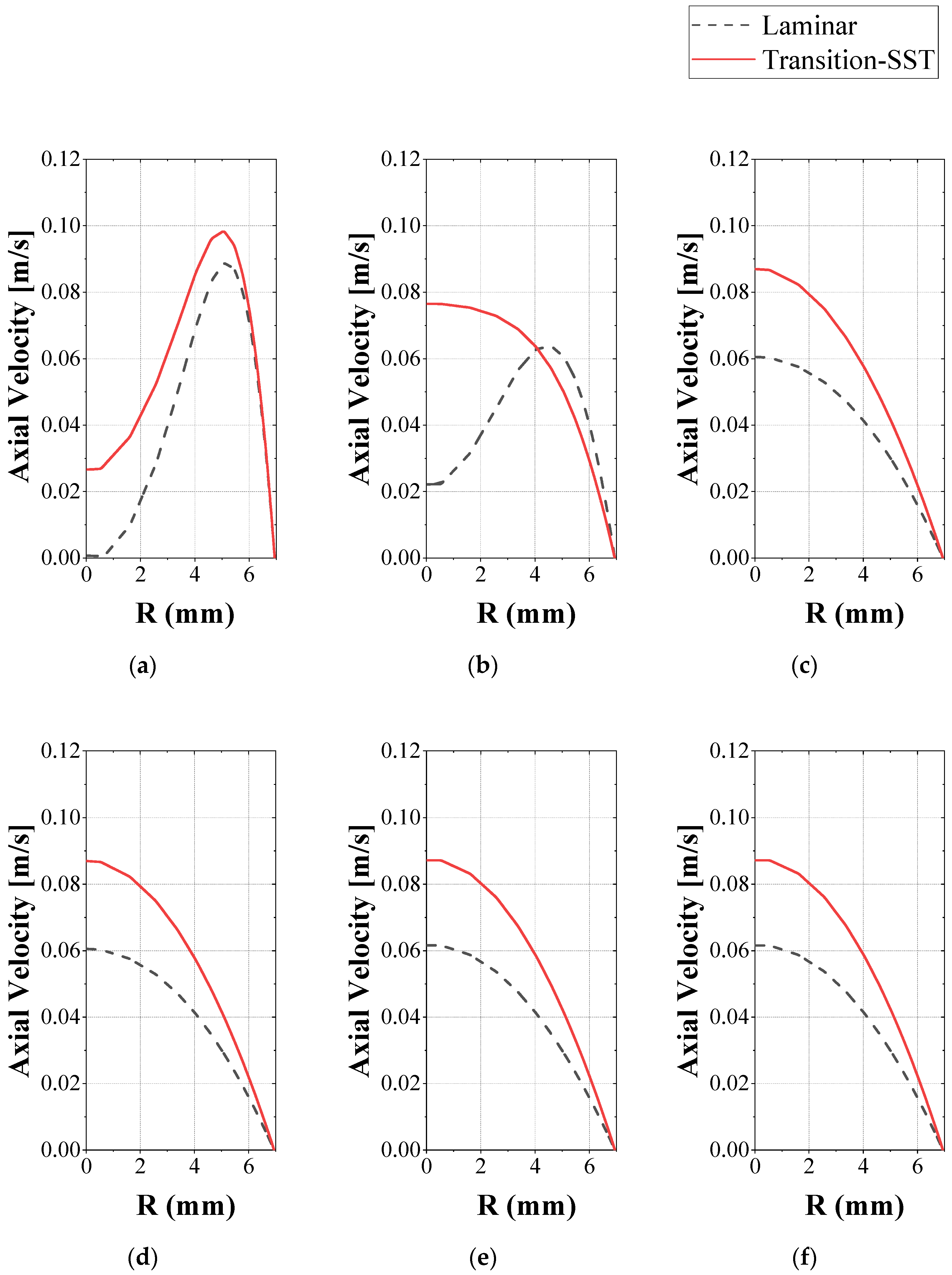
The velocity profiles in the remaining legs—the vertical-right leg and the bottom horizontal leg—are shown in Figure 14. Following Figure 12a for vertical left leg, Figure 14a–c compares the axial-velocity distributions at three vertical locations along the right leg of the loop: (a) 0.75 m above the mid height, (b) at the mid height, and (c) 0.75 m below the mid-height. A similar approach for Figure 14d–f was plotted at the location following the schematic in Figure 13a, but for the horizontal bottom leg. The three location is namely: (d) 0.5 m on the right side of the x-axis centerline, (e) at the mid length of the horizontal bottom leg, and (c) 0.5 m to the left of the mid length.

As the flow enters the vertical right leg from the cooler section, the colder fluid adjacent to the wall becomes denser and accelerates downward, producing a strong near-wall velocity peak even though no heating is applied in this region (Figure 14, profiles a–c). This inherited density gradient interacts with gravity along the vertical direction, causing the warmer core fluid to decelerate and generating an M-shaped developing profile similar to that observed in the heated vertical leg. The Transition SST model enhances this near-wall acceleration, while the laminar model diffuses it and exaggerates the low-velocity core. As the flow moves downward (profiles b–c), thermal mixing gradually reduces the wall-to-core temperature difference, and the velocity profile transitions toward a more parabolic shape as buoyancy effects weaken. After the bend into the bottom horizontal leg (profiles d–f), the temperature gradient acts vertically while the main flow is horizontal, making buoyancy influence much weaker. Consequently, the axial velocity develops smoothly along this segment, with both models predicting increasingly similar shapes, although the Transition SST model consistently yields slightly higher peak velocities due to reduced numerical diffusion.

4.7. Turbulence Magnitude and Heating Power

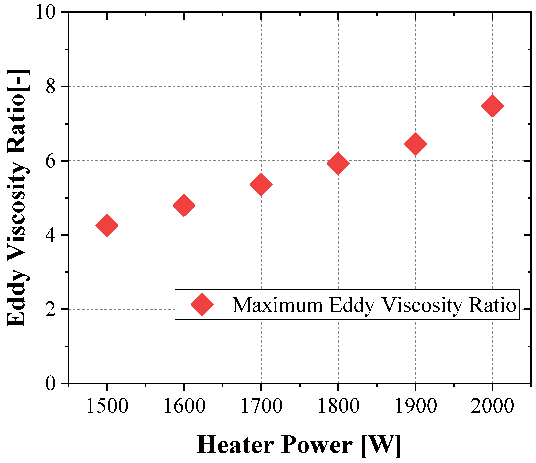
The magnitude of turbulence under different heating powers is evaluated using the eddy viscosity ratio. Figure 15 shows the variation in the maximum eddy viscosity ratio (μt/μ) in the loop as a function of heater power. The eddy viscosity ratio quantifies the relative strength of turbulence-induced momentum transport compared with molecular viscosity. In this study, the maximum value within the entire domain is extracted at each power level to illustrate how turbulence intensity evolves as thermal input increases.

As shown in Figure 15, the maximum eddy viscosity ratio increases steadily with heater power. At lower power levels, the ratio remains small, indicating that buoyancy-driven circulation is largely laminar with only weak turbulent contributions. As power increases, buoyancy forces strengthen, producing larger velocity gradients and sharper thermal stratification—particularly in the vertical legs—leading to enhanced turbulent transport. This behavior also explains why the turbulence-related error range increases at higher powers. The observed trend demonstrates that the eddy viscosity ratio is a useful indicator for diagnosing turbulence development in natural circulation loops: while the Reynolds number reflects the overall circulation strength, the eddy viscosity ratio reveals localized increases in mixing intensity. Although further investigation would be needed to quantify the stability threshold, the continuous rise in μt/μ with heating power might suggest that the loop gradually approaches a stability limit, beyond which buoyancy-driven instabilities or oscillatory behavior may emerge, as reported in earlier studies [25,27].

4.8. Future Works

Future work may extend the present 2D framework to a full 3D transient Transition SST model to better resolve flow features that cannot be captured in two dimensions, such as secondary flows and enhanced mixing in the bending sections. Benchmark studies comparing different turbulence-modeling approaches would also be valuable for clarifying how various models differ in their ability to capture transitional characteristics within the loop. Further investigation into how specific geometric parameters influence turbulence generation or suppression, together with exploring the relationship between turbulence quantities and the onset of flow instability, may provide deeper insight into stability limits and operating margins in natural circulation systems.

5. Conclusions

This study presented a two-dimensional CFD investigation of a molten salt natural circulation loop and comparison against published experimental benchmark data. Both laminar and Transition SST turbulence models were evaluated to assess their ability to reproduce global and local flow behavior. As this work is based on a two-dimensional modeling framework, the findings should be interpreted within that scope, and the applicability of the Transition SST model reflects its previously documented performance in the literature rather than a universal validation for all natural circulation systems. The key conclusions of the study are summarized below.

• Three meshes (coarse, medium, and fine) were evaluated to confirm grid independence. Transient-averaged temperature and velocity showed only minor differences across meshes, and local radial profiles demonstrated consistent shapes at each refinement level. Quantitative verification using MAE, RMSE, and MAPE confirmed that errors remained small for temperature and velocity. For the transient model, turbulence variables (eddy viscosity ratio, turbulent kinetic energy, and intermittency) were also examined. Although these quantities exhibited larger numerical variation than temperature or velocity, their local distributions remained consistent across meshes, supporting overall mesh-independent behavior.
• Both the laminar and Transition SST models reproduced the measured temperature difference across the loop with good accuracy in steady-state and transient simulations.
• Model predictions were compared with experimental velocity and Reynolds-number measurements. The laminar model underpredicted both quantities by approximately 30%, whereas the Transition SST model reduced the error to 11.8% for Reynolds number and 4.2% for velocity. The larger apparent error in the Reynolds number arises because its calculation accumulates uncertainties from several temperature-dependent properties—particularly viscosity, which is highly temperature-sensitive due to its third-order polynomial correlation.
• Temperature-dependent density and viscosity variations were examined to verify the applicability of the Boussinesq approximation. The computed Rayleigh numbers and the ratio of density to operating density remained within ranges recommended in the literature, indicating that the Boussinesq approach is valid for the operating conditions considered.
• The system’s global behavior was compared against an established Reynolds–Grashof natural circulation correlation. The correlation overpredicted the loop’s circulation strength across the tested power range, whereas the Transition SST model showed significantly closer agreement with the experimental Reynolds number. In contrast, the laminar model consistently underpredicted the circulation, confirming that turbulence modeling is necessary for accurate global-flow prediction.
• Local velocity profiles were analyzed throughout the loop to examine flow development. Both models produced similar shapes in fully developed regions, but significant differences emerged where the flow remained developing. Transition SST consistently predicted higher velocities in developing zones, reflecting its ability to resolve shear-dependent momentum transport. The analysis also showed that two factors govern the shift between developing and re-laminarizing behavior: (i) the presence of a local temperature gradient and (ii) whether the flow direction is aligned with gravity. Strong vertical temperature gradients in vertical legs promoted developing or transitional behavior, whereas regions with weak gradients or horizontal flow tended toward re-laminarization.
• The eddy viscosity ratio increased with heater power, indicating a strengthening of transitional turbulence. This trend explains why the Transition SST model provides more accurate predictions of velocity and Reynolds number at higher power levels.