Solar Photovoltaic System Fault Classification via Hierarchical Deep Learning with Imbalanced Multi-Class Thermal Dataset

Abstract

The growing global reliance on solar photovoltaic (PV) systems requires robust, automated inspection techniques to ensure reliability and efficiency. Thermal infrared (IR) imaging is widely used for detecting PV faults; however, accurate classification remains challenging due to severe class imbalance, low thermal contrast, and high inter-class visual similarity among fault types. This study proposes a hierarchical deep learning framework for thermal PV fault classification, integrating a multi-class dataset-balancing strategy to enhance representational efficiency. The proposed framework consists of two major components: (i) a hierarchical two-stage classification scheme that mitigates data imbalance and leverages limited labeled data for improved fault discrimination; and (ii) a contrast-preserving MixUp augmentation technique designed explicitly for low-contrast thermal imagery, improving minority fault class recognition and overall robustness. Comprehensive experiments were conducted on benchmark 8-class thermal PV datasets using nine deep network architectures. Dataset refactoring decisions are validated through quantitative inter-class distance analysis using multiple complementary metrics. Results demonstrate that the proposed hierarchical SlantNet model achieves the best trade-off between accuracy and computational efficiency, achieving an F1-Efficiency Index of 337.6 and processing 42,072 images per second on a GPU, over twice the efficiency of conventional approaches. Comparatively, the Swin-T Transformer attained the highest classification accuracy of 89.48% and F1 score of 80.50%, while SlantNet achieved 86.15% accuracy and 73.03% F1 score with substantially higher inference speed, highlighting its real-time potential. Ablation studies on augmentation and regularization strategies confirm that the proposed techniques significantly improve minority class detection without compromising overall performance, with detailed per-class precision, recall, and F1 analysis. The proposed framework delivers a high-accuracy, low-latency, and edge-deployable solution for automated PV inspection, facilitating seamless integration into operational PV plants for real-time fault diagnosis.

1. Introduction

The rapid growth in global energy demand, driven by population growth, industrialization, and technological advancement, has intensified pressure on conventional energy resources [1,2]. The U.S. Energy Information Administration (EIA) projects that global electricity generation will increase by 30–76% by 2050 relative to 2022, underscoring the urgent need for scalable, sustainable alternatives [3,4]. Among renewable energy sources, solar photovoltaic (PV) power has emerged as a key clean energy technology, accounting for approximately 3.6% of global electricity and playing an increasingly central role in the energy mix alongside wind power. Over the past three decades, a 99% reduction in PV manufacturing costs has enabled massive deployment, making solar a cornerstone of the clean energy transition [5].

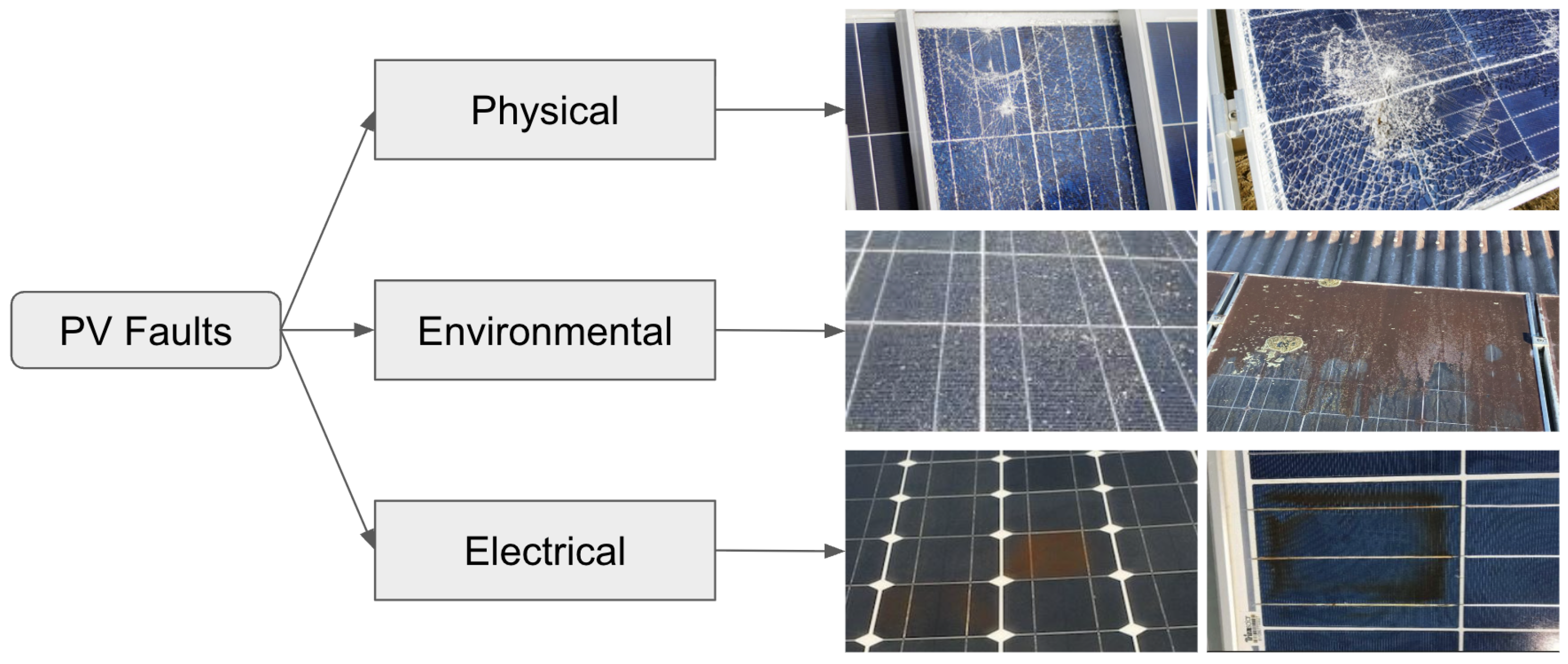
Despite these advantages, PV systems face harsh outdoor conditions that can lead to faults, degrade performance, lower energy output, and create safety hazards, including fire risk. Field studies show that undetected PV faults can result in annual power losses of up to 18.9%, underscoring the need for reliable monitoring and maintenance [6,7]. Common PV faults include hotspots (temporary or permanent), cracked cells, partial or total shading, short- and open-circuit conditions, activated bypass diodes, and soiling such as dust, bird droppings, snail trails, and delamination. These faults can be broadly categorized as electrical (e.g., open/short circuits), environmental (e.g., shading or soiling), and physical (e.g., cracks or glass breakage) [1,8], as illustrated by Figure 1.

To sustain optimal energy yield and minimize costly downtime, efficient fault detection and classification have become essential for large-scale PV plants [5,7]. Traditional PV fault detection methods fall into two main categories: electrical and non-electrical techniques. Electrical methods, such as voltage and current measurement (VCM), I–V curve analysis (I–VCA), power loss analysis (PLA), and statistical signal processing (SSP), rely on electrical parameters to identify faults in strings or modules [10,11,12,13,14]. While effective in controlled settings, these approaches often cannot precisely localize faults within individual modules and require physical access to the panels, making them impractical for large, remote PV farms [15,16].

In contrast, non-electrical techniques, especially thermal infrared (IR) imaging, provide a non-invasive, scalable alternative for PV inspection [17,18]. Thermal imaging allows the detection of anomalies, such as hotspots, cracks, and bypass-diode activation, by visualizing temperature differences across modules [19,20]. When used with unmanned aerial vehicles (UAVs), thermal inspection becomes an effective tool for quick, large-scale monitoring of PV systems. However, manual analysis of thermal images is labor-intensive and time-consuming, limiting their practicality for real-time, continuous monitoring of large-scale PV installations.

Recent advances in deep learning have enabled automated thermal PV fault classification using models such as CNNs, vision transformers (ViTs), SVMs, and fuzzy logic systems [21,22,23]. These methods can automatically detect and categorize faults such as hotspots, cracks, shading, and circuit issues using thermal patterns, thereby enhancing safety, efficiency, and early fault detection. Convolutional neural networks with transfer learning have achieved high accuracy on benchmark datasets [22,24], while lightweight architectures such as MobileNetV3 [25], LIR-Net [26], and SlantNet [27] have demonstrated competitive performance with reduced computational overhead, making them suitable for edge deployment. The solAIr system introduced Mask R-CNN for instance segmentation in large-scale PV farms [28], and cascading decision frameworks have been proposed to address data imbalance in UAV-acquired thermal datasets [29]. Furthermore, Oulefki et al. [8] developed an approach to detect anomalies in solar PV systems by combining unsupervised sensing algorithms with 3D Augmented Reality, demonstrating the promise of real-time, automated PV module maintenance using drones. However, these approaches typically report overall accuracy metrics that can mask poor performance on minority classes, and few explicitly address the multiclass imbalance problem that characterizes real-world PV inspection scenarios [30,31].

Despite these advances, multiclass thermal PV fault classification faces three significant challenges in real-world settings [32,33,34]:

• Severe class imbalance: In field inspection datasets, healthy modules often constitute 50% or more of the samples, while critical fault classes (e.g., hotspots, diode failures, soiling) may represent fewer than 2% of the data. This imbalance biases deep learning models toward the dominant healthy class, leading to poor recall for rare but safety-critical faults and undermining the practical reliability of automated systems [35].
• Low thermal contrast: Thermal images typically exhibit lower contrast than visible-spectrum images, with fault signatures appearing as subtle temperature gradients rather than distinct visual patterns [18,36]. This makes it difficult for models to distinguish between healthy and faulty regions, especially under varying environmental conditions.
• High inter-class visual similarity: Many fault types produce nearly identical thermal patterns (e.g., single-cell vs. multi-cell defects, offline modules vs. healthy ones under certain conditions), leading to substantial confusion between classes even with sufficient training data [22,24]. Standard classification methods, which assume balanced class distributions and clear visual distinctions, often fail under these conditions.

Data augmentation is a promising method for addressing class imbalance by artificially increasing the number of underrepresented categories [37,38]. Although geometric transformations (such as flipping, rotation, and scaling) are frequently used, they offer limited diversity for thermal images, where fault signatures rely more on intensity gradients than spatial structure. MixUp [39] and its variants, such as CutMix [40], have achieved strong results in natural image classification by creating convex combinations of training samples. However, directly applying MixUp to low-contrast thermal data poses challenges: the linear interpolation in standard MixUp tends to lower image contrast, further diminishing the already subtle thermal signatures that differentiate fault categories from healthy modules and from each other.

To address class imbalance, low thermal contrast, and high inter-class similarity in thermal PV fault classification, this paper proposes a real-time hierarchical deep learning framework that integrates a multi-class dataset-balancing strategy with the fast orthogonal Slant transform to enhance representational efficiency and support edge deployment in large-scale PV plants. The framework has four main components:

• Hierarchical Two-Stage Classification: A fast, automatic, two-stage pipeline first performs binary anomaly detection (healthy vs. defective) and then fine-grained multiclass fault identification. By decoupling the dominant healthy class from the multiclass classifier, this cascade reduces bias toward majority classes. It significantly improves recall for minority faults (e.g., hotspots, diode failures, rare cracks) while maintaining high precision. Early filtering of healthy modules also reduces computational load in the second stage, enabling real-time inference.
• Contrast-Preserving MixUp Augmentation: To improve minority-class recognition on low-contrast thermal images, a contrast-preserving MixUp technique is introduced. Unlike standard MixUp, which suppresses subtle thermal gradients through linear blending, the proposed method includes a contrast optimization step that restores lost intensity variations. This ensures synthetic samples retain diagnostic, meaningful thermal patterns, enhancing model robustness without introducing unrealistic artifacts.
• Dataset Refactoring and Preprocessing: A systematic analysis of class structures in thermal PV datasets identifies visually ambiguous and semantically overlapping categories (e.g., similar hotspot patterns or indistinguishable partial shading vs. soiling). Quantitative inter-class distance analysis using multiple complementary metrics (SSIM, Fréchet distance, HOG, LBP) provides objective evidence for merging decisions. A principled category merging scheme is applied to reduce inter-class confusion while preserving diagnostically relevant distinctions. This process yields a cleaner, more balanced dataset that improves classifier convergence and generalization.
• Comprehensive Benchmark Study: An extensive evaluation of an 8-class thermal PV benchmark compares various lightweight architectures, including SlantNet, MobileNetV3, EfficientNetV2, and Swin Transformer. Detailed ablation studies examine augmentation and regularization strategies, with per-class precision, recall, and F1 analysis to characterize model behavior under class imbalance.

The framework is evaluated on an 8-class thermal PV benchmark covering common faults (hotspots, cracks, shading, soiling, short/open circuits, bypass diodes). Extensive evaluations show that the proposed framework achieves a better balance between accuracy and computational efficiency. The hierarchical SlantNet model reaches an F1-Efficiency Index of 337.6 and processes 42,072 images per second on a GPU, more than twice the efficiency of conventional approaches. Swin-T achieves the highest accuracy (89.48%) and F1 score (80.50%), while SlantNet attains 86.15% accuracy and 73.03% F1 score with much higher throughput, confirming its real-time potential. Ablation studies on augmentation and regularization strategies, together with per-class precision, recall, and F1 analysis, verify that contrast-preserving MixUp and the hierarchical design significantly boost minority-class recall without degrading overall performance. Overall, the framework offers a high-accuracy, low-latency, edge-deployable solution for automated thermal PV fault classification, enabling seamless integration into operational PV plants for real-time UAV-based inspection and continuous monitoring.

The remainder of this paper is organized as follows. Section 2 reviews related work on PV fault detection, thermal imaging diagnostics, data augmentation strategies, and neural network architectures. Section 3 details the proposed dataset refactoring, contrast-preserving augmentation, and hierarchical classification pipeline. Section 4 provides experimental results, benchmark comparisons, ablation studies, and discussions. Section 5 concludes with a discussion of findings and future research directions.

2. Background

Solar photovoltaic (PV) systems are increasingly critical in global renewable energy generation. However, their performance and reliability are significantly affected by various faults that can arise during operation. Accurate fault detection and diagnosis are therefore essential for maintaining efficiency, safety, and longevity of PV modules [18,41]. This section reviews the types of PV module faults, thermal imaging diagnostics, deep learning approaches for fault classification, data augmentation strategies, and the neural network architectures commonly employed in this domain.

2.1. Types of PV Module Faults

PV faults are generally categorized by their electrical, mechanical, or environmental origins [42,43].

Table 1. Summary of common PV module faults and their characteristics.

Fault Type	Causes and Effects	Diagnostic Priority	Occurrence
No-Anomaly	Normal operation with uniform irradiance and electrical output. Serves as a baseline for comparison.	N/A	N/A
Cell, Cell-Multi	Microcracks, broken interconnects, or cell degradation cause reduced current and localized heating. Often a precursor to hotspots.	High	5–15% [43]
Cracking	Mechanical stress, thermal cycling, or transport damage leading to increased series resistance. Thermal patterns may be subtle.	Medium	4–10% [42]
Hot-Spot, Hot-Spot-Multi	Reverse-biased cells, shading, or severe mismatch causing concentrated heating. Safety risk, including fire hazard.	Very High	10–15% [18]
Shadowing	Partial shading from buildings, vegetation, or adjacent rows causes electrical mismatch and potential hotspot formation.	High	15–20% [44]
Diode, Diode-Multi	Faulty bypass diodes or solder joints are causing localized heating and reduced string performance with pronounced thermal signatures.	High	3–8% [36]
Vegetation	Plant overgrowth produces shading or trapping soiling and moisture. Generally preventable with maintenance.	Medium	10–25% [44]
Soiling	Dust, pollen, bird droppings, or salt deposits reduce irradiance and cause uneven heating. Most common performance loss driver.	High	25–35% [45]
Offline-Module	Complete electrical disconnection or severe module failure. Shows a uniform temperature difference from the ambient.	Very High	Site-dependent [41]

Note: Occurrence rates are approximate ranges from field surveys and meta-analyses; actual frequencies depend on climate, array age, and maintenance practices.

summarizes common fault types, their causes, diagnostic importance, and typical occurrence rates reported in the literature.

2.2. Thermal Imaging for Fault Detection

Thermal infrared (IR) imaging has emerged as one of the most efficient diagnostic techniques for PV systems due to its non-invasive nature, scalability via drone-mounted cameras, and compatibility with automated deep learning methods [34,36]. Faults such as hot-spots, diode failures, and shadowing create detectable thermal signatures that can be captured remotely without electrical contact or system downtime [46]. Field surveys indicate that soiling and shading are the most prevalent faults (25–35% and 15–20%, respectively), while hot-spots and cell defects occur less frequently (10–15%) but pose greater safety risks [43,47]. Despite significant progress, challenges persist in standardizing labeling conventions, ensuring environmental robustness under different irradiance conditions, and defining universal temperature thresholds for hazard classification [34,35].

2.3. Deep Learning Approaches for PV Fault Classification

Deep learning has revolutionized fault detection and classification in PV systems, with convolutional neural networks (CNNs) demonstrating remarkable proficiency in image classification tasks [21,22,23]. Early approaches adapted pre-trained networks for thermal image analysis, while more recent work has focused on architectures specifically designed for the unique challenges of infrared imagery.

Alves et al. [22] employed CNNs with infrared thermography for multiclass defect classification, demonstrating the importance of data augmentation to handle unbalanced datasets. Cipriani et al. [48] specifically addressed dust and hotspot classification in PV modules using CNNs, achieving high accuracy in distinguishing between these common fault types. Korkmaz and Acikgoz [24] proposed a multi-scale CNN with transfer learning, using multiple convolutional branches to improve feature representation across various fault types. Their approach employed offline augmentation techniques to address dataset imbalance and achieved robust performance across fault categories, including cracks and diode failures.

The solAIr system introduced by Pierdicca et al. [28] represents a significant advancement, utilizing Mask R-CNN for instance segmentation on thermal images to detect and localize anomalies in large-scale PV farms. This approach demonstrated high accuracy in identifying and localizing faulty cells, establishing a benchmark for subsequent studies. Similarly, Ahmed et al. [33] applied transfer learning with deep neural models for PV panel classification using infrared thermographic images, while Bommes et al. [49] utilized supervised contrastive learning to address domain shift challenges between different PV installations.

Lightweight architectures have gained particular attention due to the need for real-time deployment. Pamungkas et al. [50] introduced a coupled UDenseNet model leveraging geometric transformations and GAN-based image augmentation to achieve high accuracy suitable for large-scale solar farms. Lee et al. [26] developed LIR-Net, a lightweight inception residual network incorporating hierarchical learning and K-means clustering to refine datasets and improve fault detection. Tang et al. [25] proposed modifications to MobileNet for UAV-based automatic defect identification, achieving faster inference and higher recognition rates. Beyond thermal imaging, Gasparyan et al. [51] recently showed that efficient, lightweight networks can classify faults in solar panels using electroluminescence (EL) and RGB images, emphasizing the potential of multimodal methods for thorough PV diagnostics.

Recent work has also addressed multi-modal and aerial inspection approaches for PV fault detection. Pinho et al. [52] proposed a multi-modal data fusion framework for anomaly detection in aerial PV inspections, combining thermal and RGB imagery to improve detection robustness. Qader and Albalooshi [53] introduced an attention-enhanced deep learning model for solar panel anomaly detection, demonstrating improved reliability through attention mechanisms that focus on diagnostically relevant thermal features. These advances highlight ongoing efforts to improve model robustness and interpretability in PV fault classification.

2.4. Data Augmentation Strategies for Thermal Images

Data augmentation plays a crucial role in improving model robustness, particularly when dealing with limited and imbalanced datasets common in PV fault detection [37,38]. Standard geometric transformations, including rotation, flipping, and scaling, have been widely adopted to increase training data diversity [24,50]. However, these techniques alone may be insufficient for the unique characteristics of thermal imagery.

MixUp [39] represents a paradigm shift in data augmentation by creating synthetic training examples through linear interpolation of image pairs. While effective for natural images, direct application to thermal data presents challenges: the blending process tends to reduce contrast, suppressing the already subtle thermal signatures that distinguish fault categories. CutMix [40] addresses some limitations by cutting and pasting image patches, preserving local features while increasing data diversity. RandAugment [54] offers automated augmentation policy selection, reducing the need for manual hyperparameter tuning.

Domain-specific augmentation strategies have emerged for thermal PV images. Contrast enhancement techniques guided by image quality measures have shown promise in improving model performance on low-contrast thermal data [17,55]. The foundational work on transform-based image enhancement with performance measures by Agaian et al. [56] established a principled framework for optimizing enhancement parameters using quantitative metrics rather than subjective visual assessment. Building on these principles, Ayunts et al. [57] introduced a novel entropy measure specifically designed for thermal imaging, enabling uncertainty quantification and enhanced contrast in low-resolution infrared data. These measure-driven approaches ensure that augmented samples retain the thermal intensity variations essential for accurate fault classification.

2.5. Neural Network Architectures

We evaluate architecture spanning classical CNNs, lightweight models, and vision transformers. Classical architectures include AlexNet [58] and ResNet50 [59], which provide strong baselines but are computationally intensive. Lightweight architectures designed for mobile deployment include SqueezeNet [60], ShuffleNetV2 [61], MobileNetV3 [62], and EfficientNetV2 [63], which achieve competitive accuracy with reduced computational overhead through techniques such as depthwise separable convolutions and neural architecture search.

For transformer-based approaches, Vision Transformer (ViT) [64] treats images as patch sequences but typically requires large datasets, while Swin Transformer [65] addresses this limitation through hierarchical shifted-window attention, achieving strong performance with reasonable computational cost. Finally, SlantNet [27] is a domain-specific lightweight architecture designed for thermal PV fault classification, incorporating slant convolution layers to capture directional thermal gradients with approximately 60% reduced computational overhead compared to leading models [66].

3. Proposed Method

3.1. Dataset Refactoring

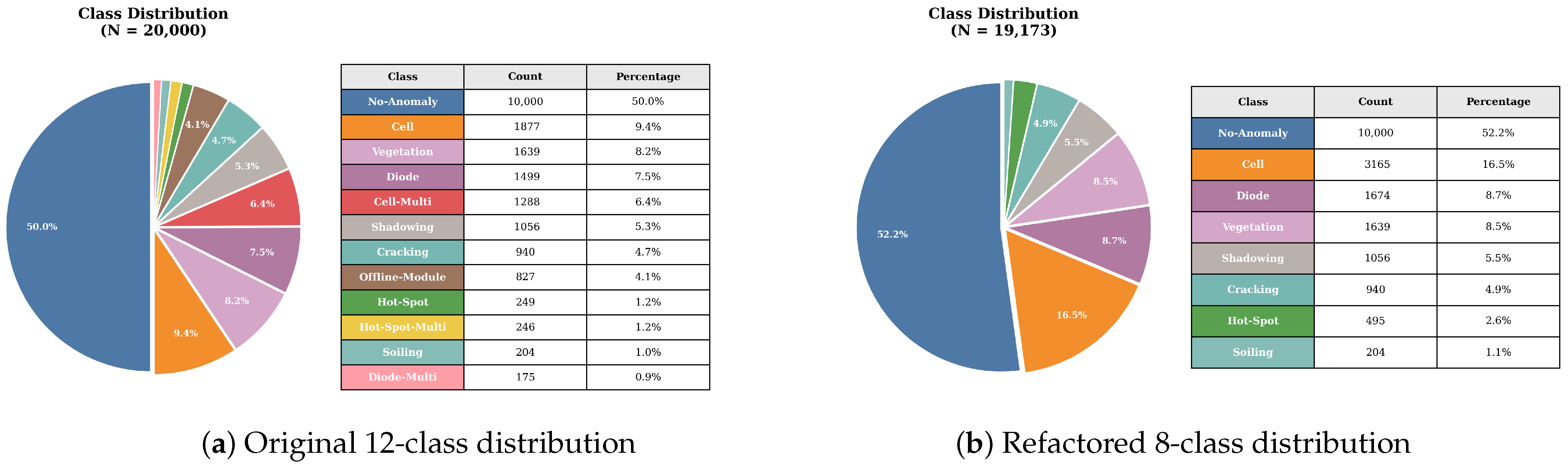
The initial dataset [32] comprises thermal infrared images of PV modules across 12 classes: No-Anomaly, Cell, Cell-Multi, Cracking, Hot-Spot, Hot-Spot-Multi, Shadowing, Diode, Diode-Multi, Vegetation, Soiling, and Offline-Module. The dataset exhibits severe imbalance with No-Anomaly comprising 50% of samples, biasing models toward the healthy class and reducing recall for rare but critical faults. Additionally, some classes represent semantically overlapping failure modes. After refactoring (Figure 2), the dataset is reduced to 8 classes by removing Offline-Module and merging multi-type variants (Cell-Multi, Diode-Multi, Hot-Spot-Multi) with their base classes.

Following dataset refactoring, we applied a stratified random split to partition the data into training, validation, and test sets with an 80/10/10 ratio. The stratification ensures that class proportions are preserved across all splits as closely as possible, given the discrete sample counts. Since the public dataset [32] does not provide metadata such as site identifiers, flight paths, or acquisition dates, site-aware or temporal splitting strategies were not feasible.

Table 2. Sample counts per class after stratified 80/10/10 split. Totals: 15,337 training/1916 validation/1920 test.

Class	Train	Val	Test	Class	Train	Val	Test
No-Anomaly	8000	1000	1000	Shadowing	844	106	106
Cell	2532	316	317	Cracking	752	94	94
Diode	1339	167	168	Hot-Spot	396	49	50
Vegetation	1311	164	164	Soiling	163	20	21

reports the exact sample counts per class for each split.

Thermal imaging plays a key role in identifying these anomalies, as temperature gradients on the panel surface indicate electrical or physical faults invisible to standard RGB inspection. However, due to the limited spectral and spatial contrast in thermal-domain images, many fault categories exhibit only subtle temperature pattern variations, which complicates model discrimination.

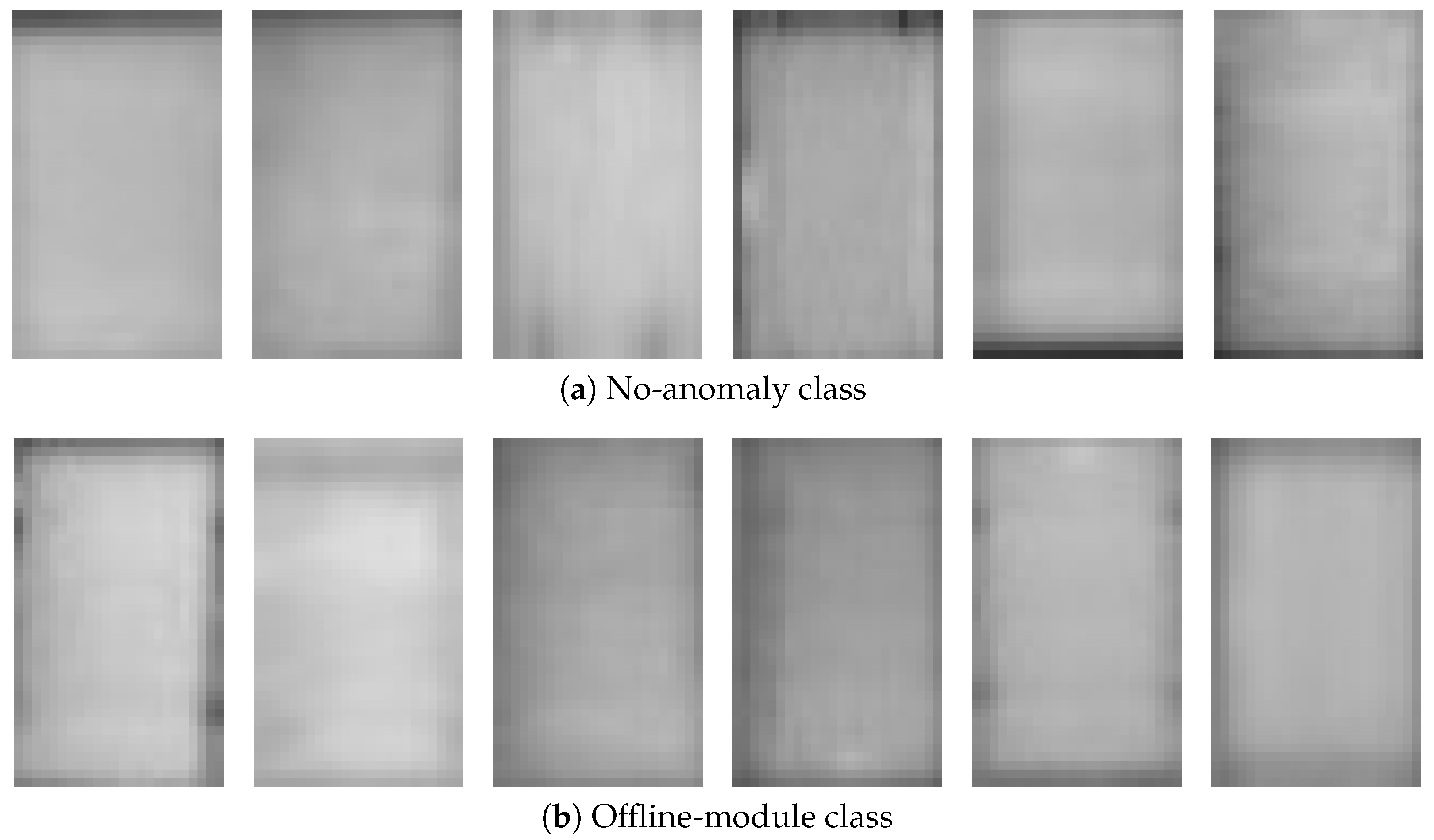
Figure 3 illustrates an example comparison between No-Anomaly and Offline-Module samples. Despite belonging to distinct classes, their thermal signatures are visually indistinguishable, particularly under varying background and ambient conditions. Because of this similarity and the relatively small sample size (827 images), the Offline-Module category was excluded from the refactored dataset to prevent confusion and improve classifier convergence.

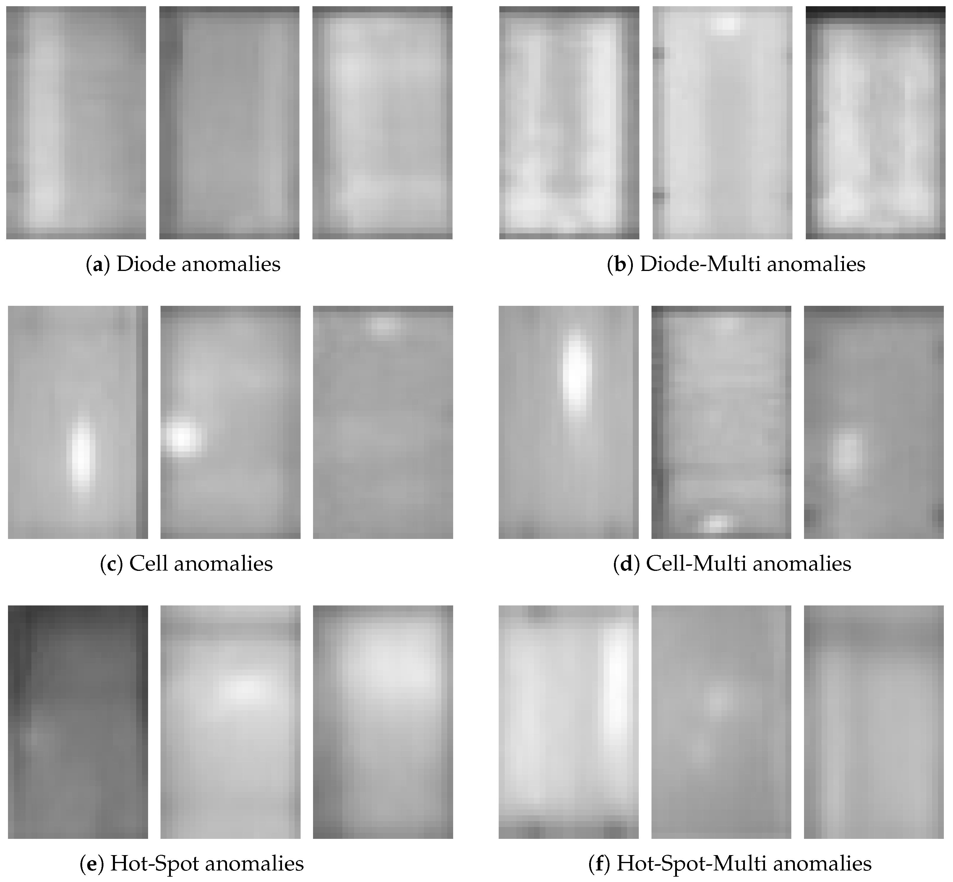
Furthermore, a detailed analysis of thermal patterns revealed substantial similarity between several “single” and “multi” fault variants, such as Diode vs. Diode-Multi, Cell vs. Cell-Multi, and Hot-Spot vs. Hot-Spot-Multi. As illustrated in Figure 4, these pairs share nearly identical heat distribution and structural features, differing primarily in spatial extent rather than type. Given their low sample counts and high similarity, each multi-type was merged with its corresponding base class (e.g., Diode + Diode-Multi) to reduce class fragmentation and increase intra-class variability.

To quantitatively validate the merging decisions, we computed inter-class distances using five complementary similarity metrics spanning pixel-level, texture-level, and deep feature representations.

Table 3. Inter-class similarity metrics used for dataset refactoring analysis.

Metric	Type	Feature Level	Captures	Reference
SSIM ↑	Similarity	Pixel	Luminance, contrast, and structural patterns	Wang et al. [67]
Fréchet ↓	Distance	Deep (ResNet-18)	Feature distribution difference (FID-like)	Heusel et al. [68]
Cosine ↓	Distance	Deep (ResNet-18)	Angular separation in feature space	–
HOG ↓	Distance	Texture	Histogram of edge orientations	Dalal & Triggs [69]
LBP ↓	Distance	Texture	Local binary texture patterns	Ojala et al. [70]

summarizes the metrics employed in this analysis.

Table 4. Inter-class similarity analysis for merge candidates. Percentages indicate the fraction of all class pairs with lower similarity (higher distance). ↑: higher is more similar; ↓: lower is more similar.

Class Pair	SSIM ↑	Fréchet ↓	Cosine ↓	HOG ↓	LBP ↓
Cell ↔ Cell-Multi	0.715 (65%)	5.54 (98%)	0.0019 (98%)	0.73 (97%)	0.0011 (86%)
Diode ↔ Diode-Multi	0.735 (91%)	8.09 (91%)	0.0029 (94%)	1.05 (83%)	0.0009 (92%)
Hot-Spot ↔ Hot-Spot-Multi	0.726 (74%)	11.66 (66%)	0.0086 (52%)	2.29 (18%)	0.0018 (66%)
No-Anomaly ↔ Offline-Module	0.738 (92%)	11.74 (65%)	0.0065 (66%)	0.97 (92%)	0.0057 (29%)

presents the inter-class distances for the four merge candidates. Values in parentheses indicate the percentile ranking, i.e., the percentage of all 66 class pairs with larger (less similar) distances. Higher percentiles indicate stronger evidence for merging.

The quantitative analysis reveals that Cell ↔ Cell-Multi and Diode ↔ Diode-Multi exhibit consistently high similarity across all metrics (83–98% percentile), strongly supporting their merger. The Hot-Spot ↔ Hot-Spot-Multi pair shows more moderate similarity, particularly in HOG distance (18% percentile), suggesting greater visual variability; however, the semantic equivalence of these fault types justifies merging to increase sample diversity. For No-Anomaly ↔ Offline-Module, the high SSIM (92%) and HOG (92%) similarity confirms that these classes are visually indistinguishable, supporting the removal of Offline-Module to prevent classifier confusion.

Notably, the analysis also revealed that some semantically unrelated classes exhibit unexpectedly high similarity. For instance, Cell ↔ Vegetation achieves the highest cosine similarity (0.0012) among all pairs, and Hot-Spot ↔ No-Anomaly shows the highest SSIM (0.752). Such cross-category similarities highlight the low thermal contrast inherent in this imaging domain and underscore the classification challenge posed by subtle inter-class boundaries.

As reported in our recent work [27], these inter-class similarities were among the main causes of low recall and misclassification in convolutional and transformer-based models. By refactoring the dataset to remove redundant categories and merge overlapping ones, we effectively reduced confusion during training and improved the discriminative consistency of the thermal patterns. This restructuring step proved essential for achieving more balanced and reliable classification performance across diverse PV fault types.

3.2. Dataset Augmentation

After the dataset refactoring described in the previous subsection, several classes still remained significantly underrepresented. In particular, Hot-Spot (495 images) and Soiling (204 images) were vastly smaller compared to the dominant categories, such as No-Anomaly (10,000 images) and Cell (3165 images). Such an imbalance not only skews the training process but also decreases the classifier’s ability to generalize when identifying rare but important anomalies. To address this issue, we are introducing a dataset augmentation strategy based on a modified offline MixUp procedure.

Importantly, all augmentation operations are performed exclusively on the training set after the train/validation/test split has been finalized. No validation or test images are used in the MixUp procedure, and synthetic samples are generated solely from within-class training pairs. This strict separation ensures that no data leakage occurs between splits, preserving the integrity of the evaluation protocol.

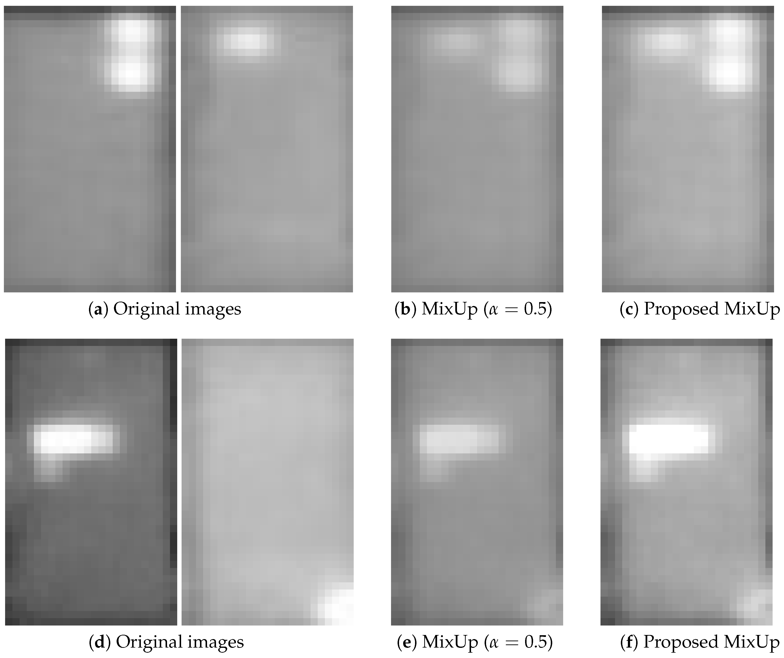
MixUp is commonly used to increase data diversity by linearly interpolating pairs of images. However, directly applying MixUp to low-contrast thermal images has an undesirable side effect: the resulting blended images often exhibit reduced contrast, which suppresses the already subtle signatures of PV anomalies. This is particularly detrimental for defects such as Hot-Spot, Soiling, or Diode, where thermal intensity differences are small. We empirically observed that classical MixUp produces overly smooth images where defect regions become barely distinguishable. Therefore, a contrast-preserving augmentation strategy is required.

Our proposed method extends offline MixUp by (1) restricting the mixing ratio to a range that avoids excessive dilution of defect intensity, and (2) applying a contrast optimization step that restores detail after mixing. This second step is the key innovation: for each mixed image, we search for contrast stretching parameters that minimize the difference between the contrast of the parents and the augmented output. Following our earlier work [57], we use the standard deviation of pixel intensities as a contrast measure and employ a simple metaheuristic search over stretching bounds to maximize contrast preservation. This ensures that augmented samples remain visually plausible and diagnostically informative.

The theoretical motivation for this approach stems from the observation that standard MixUp with mixing ratio $\lambda$ produces blended images whose contrast decreases approximately as $\sqrt{{\lambda }^2+{(1-\lambda )}^2}$ relative to the parent images, assuming uncorrelated pixel intensities. For $\lambda =0.5$, this yields a contrast reduction of approximately 29%. In thermal imagery where fault signatures already exhibit low contrast (typically 5–15% intensity variation above background), this additional reduction can push diagnostic features below the perceptual threshold. Our contrast restoration step explicitly compensates for this degradation by matching the output contrast to the maximum of the parent contrasts, thereby preserving the thermal gradient information essential for fault detection. The choice of standard deviation as the contrast metric is grounded in its direct relationship to the Root Mean Square (RMS) contrast widely used in image quality assessment [71], while being computationally efficient for real-time augmentation pipelines.

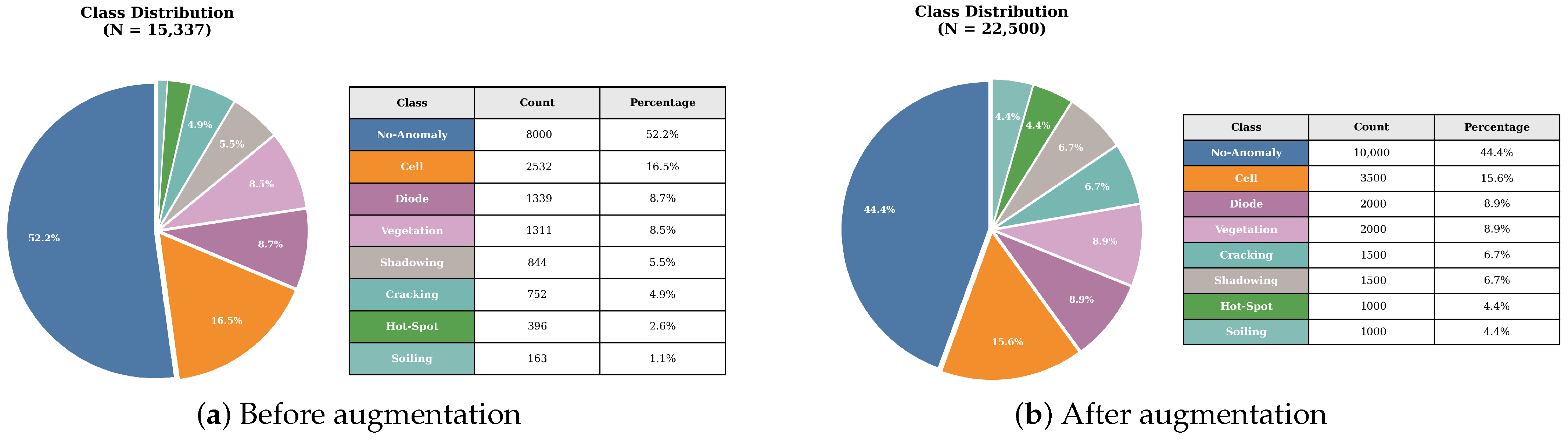
The final augmentation pipeline also incorporates random geometric flips to introduce spatial variability. Class-specific target sizes are set based on original class frequencies: the dominant No-Anomaly class is capped at 10,000 images, Cell at 3500, Diode and Vegetation at 2000, Cracking and Shadowing at 1500, and the smallest classes Hot-Spot and Soiling at 1000 each, resulting in a total training set of 22,500 images. This augmentation configuration was used consistently across all experiments; the validation and test sets remained fixed and unaugmented throughout. For the “No Aug” ablation study (Section 4.4), we used the original unaugmented training set (15,337 images) while keeping the same validation and test splits. Figure 5 shows the training set class distribution before and after applying the proposed contrast-preserving MixUp augmentation, demonstrating the significant balancing effect on underrepresented fault categories.

Figure 6 illustrates two representative examples of Soiling anomalies augmented with standard MixUp ($\alpha =0.5$) and with our proposed contrast-optimized variant. The standard MixUp output visibly reduces the temperature gradients that characterize soiling defects, resulting in overly smoothed textures in which anomaly regions are difficult to distinguish from the background. In contrast, our optimization procedure restores the thermal contrast to a level comparable to, or in some cases higher than, the more informative parent image. This preserves the local intensity variations that neural networks rely on to detect faults.

A concise pseudocode representation of the proposed augmentation process is presented in Algorithm 1.

Algorithm 1 Contrast-Preserving MixUp Augmentation for Thermal PV Images

Require:  Dataset $\mathcal{D}$ with per-class image sets ${\left\{{\mathcal{D}}_c\right\}}_{c=1}^C$ Require:  MixUp shape parameter $\alpha$, mix range $[r_{min},r_{max}]$ Require:  Target sizes ${\left\{T_c\right\}}_{c=1}^C$ for each class Ensure:  Augmented dataset ${\mathcal{D}}^{\prime }$ with balanced class distribution  1: for each class $c\in \{1,\dots ,C\}$ do  2:       while $|{\mathcal{D}}_c| <T_c$ do  3:          Sample two images: $I_1,I_2\sim {\mathcal{D}}_c$  4:          Apply random horizontal/vertical flips to $I_1$ and $I_2$  5:          Sample $r\sim \mathrm{Beta}(\alpha ,\alpha )$  6:          Scale to range: $r\leftarrow r_{min}+r·(r_{max}-r_{min})$  7:          Mix images: $I_m\leftarrow r·I_1+(1-r)·I_2$  8:          Compute target contrast: ${\sigma }^{*}\leftarrow max\left(\mathrm{STD}\left(I_1\right),\mathrm{STD}\left(I_2\right)\right)$  9:          Optimize: $I_m^{*}\leftarrow arg{min}_{s\in \mathcal{S}}\left|{\sigma }^{*}-\mathrm{STD}\left(\mathrm{stretch}(I_m,s)\right)\right|$ 10:          Apply random flip to $I_m^{*}$ 11:          Add $I_m^{*}$ to ${\mathcal{D}}_c$ 12:       end while 13: end for 14: return  ${\mathcal{D}}^{\prime }\leftarrow {\bigcup }_{c=1}^C{\mathcal{D}}_c$

3.3. Hierarchical Pipeline for Solar Panel Anomaly Detection

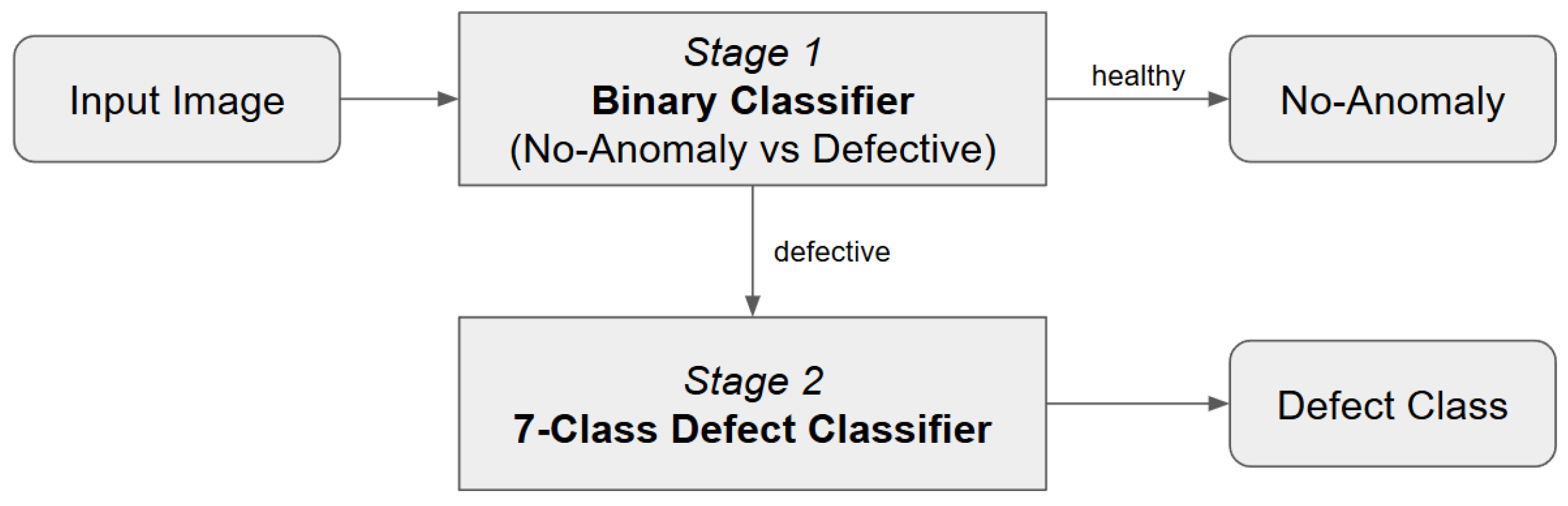
We adopt a hierarchical two-stage architecture (Figure 7) to mitigate class imbalance and reduce inter-class confusion. The first stage is a binary classifier distinguishing No-Anomaly from Defective, acting as a coarse filter that prevents the multiclass classifier from being overwhelmed by the dominant healthy class. Detected defects are forwarded to the second stage, which performs seven-class classification among fault categories: Cell, Diode, Cracking, Hot-Spot, Shadowing, Vegetation, and Soiling.

Both stages share the same backbone architecture, differing only in output neurons, making the pipeline model-agnostic and compatible with any CNN or transformer backbone. This cascade improves recall for rare defects by eliminating competition with the dominant healthy class and allows the second stage to focus entirely on distinguishing fault types [27].

4. Results and Discussion

This section presents a thorough evaluation of the proposed framework. We begin by outlining the experimental setup and the metrics used for performance assessment. An in-depth analysis of the quantitative results follows. Furthermore, we provide ablation studies to isolate and examine the individual impact of the hierarchical classification strategy and the proposed augmentation method. Finally, we assess the computational efficiency of the framework and compare it with representative baseline approaches.

4.1. Experimental Setup

All experiments were performed on a high-performance workstation equipped with an NVIDIA GeForce RTX 4070 Ti SUPER GPU (12 GB GDDR6X), providing ample computational capacity for deep learning training and large-scale inference. The system was powered by an Intel Core i7-13700K processor with 16 cores (8 performance and 8 efficiency cores) and a boost clock of 5.4 GHz, supported by 32 GB of DDR5 RAM. This hardware configuration ensured the stable execution of memory-intensive workloads, efficient data loading, and reliable benchmarking of all evaluated models.

To maintain consistency across experiments, the same set of hyperparameters was applied to both stages of the hierarchical classification system. Each model was trained for up to 50 epochs using Cross-Entropy loss, with model selection based on the lowest validation loss. Optimization was performed with the AdamW optimizer, which includes weight decay to improve generalization. A batch size of 32 was used to balance computational efficiency and gradient stability. A CosineAnnealingLR scheduler was employed with $T_{max}=50$ (equal to the number of epochs) to gradually reduce the learning rate from its initial value to a minimum of ${\eta }_{min}=1\times {10}^{-6}$ over the training period, promoting smoother convergence.

Initial learning rates were $1\times {10}^{-3}$ for binary classification and $5\times {10}^{-4}$ for multiclass fault classification, reflecting the increased complexity of distinguishing visually similar fault categories where a smaller learning rate helps learn more refined decision boundaries.

Direct comparison with prior PV-specific thermal fault classification methods faces significant reproducibility barriers. First, publicly available open-source thermal PV fault datasets remain extremely scarce; to our knowledge, the dataset used in this study [32] is the only openly accessible multiclass benchmark for this domain. Second, existing PV-specific classifiers rarely provide open-source code, pretrained weights, or detailed training protocols necessary for faithful reproduction. Third, prior works often use proprietary or unpublished datasets with different class taxonomies, imaging sensors, and environmental conditions, making direct metric comparisons misleading. Given these constraints, we benchmark our method against strong, well-documented general-purpose architectures with publicly available implementations, ensuring reproducibility and fair evaluation. We include the SlantNet model from our previous work [27] and representative CNN and Transformer baselines. Specifically, we selected MobileNetV3, EfficientNetV2, and Swin Transformer (tiny) to ensure a fair, efficient, and contemporary comparison with the proposed framework. The above hyperparameters were applied to all CNN-based models; for transformer-based architectures (ViT and Swin), we used the same configuration with learning rates tuned according to their respective original implementations.

4.2. Evaluation Metrics

Classification performance is evaluated using standard metrics [72]: accuracy, precision, recall (sensitivity), F1 score, and specificity (

Table 5. Summary of evaluation metrics used for PV fault classification [72].

Metric	Formula	Description
Accuracy	${\displaystyle \frac{TP+TN}{TP+TN+FP+FN}}$	Overall proportion of correct predictions. Misleading under the class imbalance.
Precision	${\displaystyle \frac{TP}{TP+FP}}$	Correctness of positive predictions; high precision implies low false-positive rate.
Recall (Sensitivity)	${\displaystyle \frac{TP}{TP+FN}}$	Ability to detect actual faults; high recall indicates few missed defects.
F1 Score	${\displaystyle \frac{2\times \mathrm{Pr}\times \mathrm{Rec}}{\mathrm{Pr}+\mathrm{Rec}}}$	Harmonic mean of precision and recall; useful for imbalanced datasets.
Specificity (TNR)	${\displaystyle \frac{TN}{TN+FP}}$	Ability to correctly identify non-faulty modules, reducing false alarms.

). We emphasize F1 score as the primary metric since accuracy can be misleading under class imbalance, while F1 balances precision (correctness of fault predictions) and recall (ability to detect actual faults). Specificity reflects how reliably the model identifies healthy modules, reducing false alarms.

Computational efficiency is evaluated following [66]: trainable parameters (P, millions), FLOPs (MMac), memory footprint (M, MB), throughput (T, images/second), and latency (L, ms/image). To unify classification and efficiency, we introduce the F1-Efficiency Index (FEI):

$$\mathrm{FEI}=\mathrm{F}1\times {log}_{10}\left(T\right),$$

(1)

where the F1 score is used instead of accuracy due to class imbalance. The logarithmic throughput term ensures each order-of-magnitude speed increase contributes equally, meeting the practical need for real-time UAV-based inspection where systems must process thousands of images efficiently [28,73]. Alternative formulations (e.g., natural logarithm or F1 in $[0,1]$) scale FEI by constant factors without affecting model rankings. As with any composite metric, FEI values are dataset-dependent and should be interpreted within the specific benchmark context.

4.3. Quantitative Results

Table 6. Binary classification performance (Best F1 Model) on validation and test sets. Best metrics in bold.

Model	Test					Validation
	Acc	Pr	Rec	F1	Sp	Acc	Pr	Rec	F1	Sp
AlexNet	94.74	95.65	93.26	94.44	96.10	94.78	95.33	93.67	94.49	95.80
ResNet-50	94.11	95.70	91.85	93.73	96.20	94.10	95.78	91.70	93.70	96.30
SqueezeNet	93.28	92.94	93.04	92.99	93.50	93.58	93.62	92.90	93.26	94.20
ShuffleNet-V2	94.22	95.20	92.61	93.88	95.70	94.73	95.03	93.89	94.45	95.50
MobileNet-V3	96.41	97.86	94.57	96.19	98.10	96.29	97.96	94.21	96.05	98.20
EfficientNet	96.04	97.85	93.80	95.78	98.10	95.72	97.49	93.45	95.43	97.80
ViT-B/16	90.94	90.28	90.87	90.57	91.00	90.29	89.42	90.39	89.90	90.20
Swin-T	96.25	96.59	95.54	96.06	96.90	96.45	96.49	96.07	96.28	96.80
SlantNet	95.89	97.09	94.24	95.64	97.40	95.77	96.23	94.87	95.55	96.60

and 

Table 7. Hierarchical classification performance (Best F1 Model) on validation and test sets. Best metrics in bold.

Model	Test					Validation
	Acc	Pr	Rec	F1	Sp	Acc	Pr	Rec	F1	Sp
AlexNet	84.38	70.54	69.30	69.90	97.43	85.18	73.62	73.11	73.30	97.57
ResNet-50	85.16	73.29	72.53	72.78	97.47	85.07	74.68	75.06	74.45	97.45
SqueezeNet	82.14	66.52	67.67	66.77	97.13	82.99	70.22	72.37	70.61	97.22
ShuffleNet-V2	85.21	73.47	71.92	72.64	97.52	85.33	74.08	73.97	73.85	97.60
MobileNet-V3	87.60	76.27	75.17	75.65	97.97	87.42	76.92	77.50	77.04	97.92
EfficientNet	87.76	78.22	75.67	76.47	97.94	87.47	77.60	76.22	76.53	97.87
ViT-B/16	77.81	59.91	61.56	60.56	96.41	77.82	60.88	63.27	61.95	96.38
Swin-T	89.48	80.83	80.33	80.50	98.28	88.99	82.21	82.71	82.29	98.23
SlantNet	86.15	74.87	71.66	73.03	97.74	86.22	76.21	75.66	75.61	97.78

summarize the quantitative performance of all evaluated models on both the validation and test sets. Table 6 presents the binary classification results (healthy vs. defective), while Table 7 reports the hierarchical 8-class classification performance. The reported metrics include accuracy (Acc), precision (Pr), recall (Rec), F1 score, and specificity (Sp), providing a comprehensive view of each model’s effectiveness in detecting and distinguishing photovoltaic module anomalies. For binary classification, MobileNet-V3 achieves the highest test accuracy (96.41%) and F1 score (96.19%), while Swin-T demonstrates the best recall (95.54%). In the more challenging hierarchical task, Swin-T consistently outperforms all other models across all metrics, achieving 89.48% accuracy and 80.50% F1 score on the test set. Notably, ViT-B/16 struggles significantly with the thermal PV data, suggesting that standard vision transformers require larger datasets or domain-specific pretraining for this application.

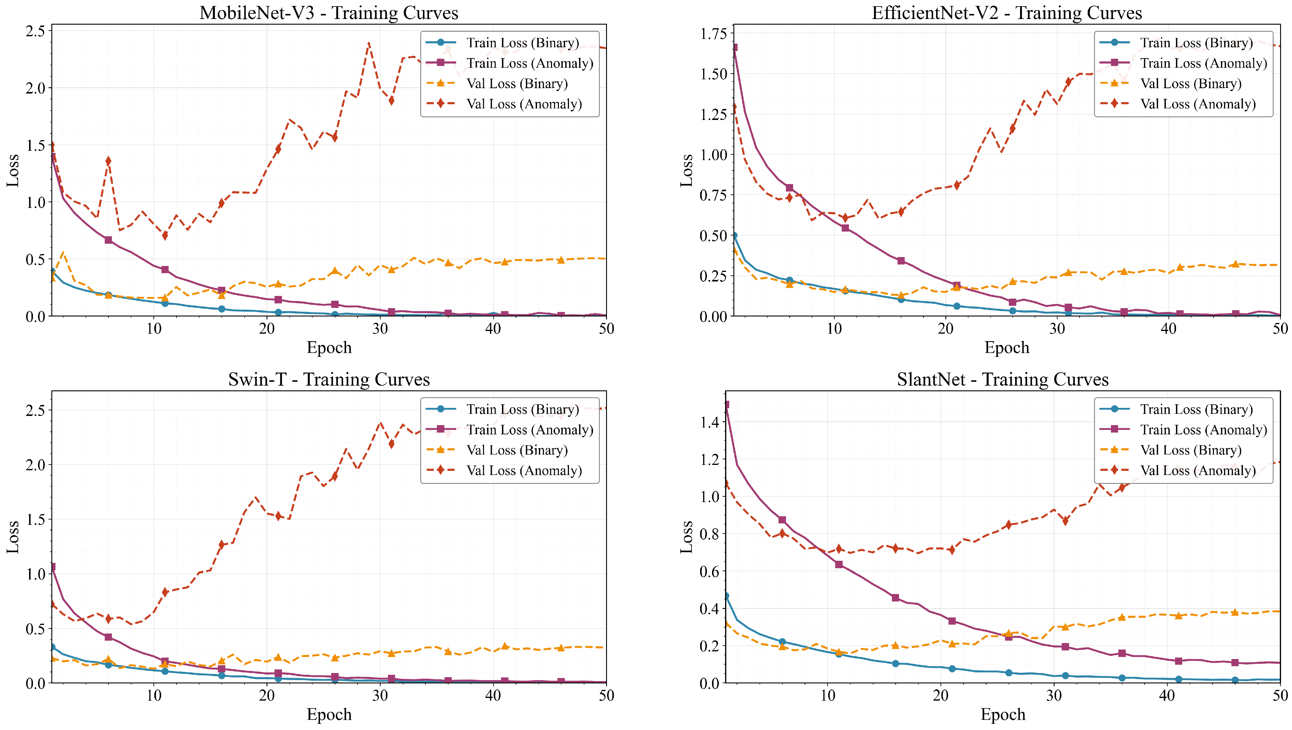
Figure 8 illustrates the training and validation loss curves for four representative models: MobileNet-V3, EfficientNet-V2, Swin-T, and SlantNet. Each subplot displays the loss progression for both the binary classifier (blue/orange) and anomaly classifier (purple/red) over 50 epochs. A notable observation across all models is the divergence between training and validation losses for the anomaly classifier, indicating the inherent difficulty of multiclass fault discrimination. While training losses consistently decrease, validation losses for the anomaly task tend to increase after initial convergence, suggesting overfitting to the training distribution. SlantNet exhibits the most stable convergence behavior with minimal overfitting, while MobileNet-V3 and EfficientNet-V2 show more pronounced validation loss divergence in the anomaly task.

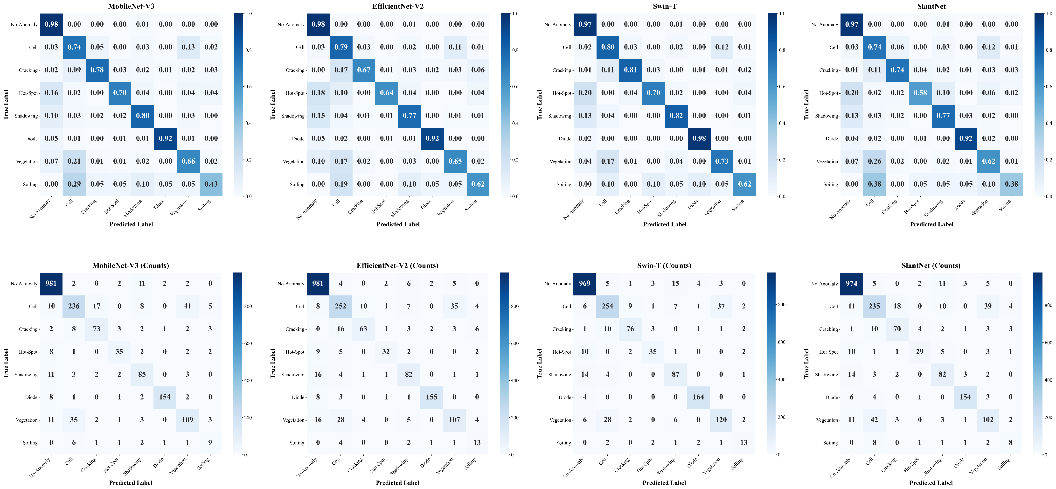
Figure 9 presents the normalized confusion matrices for the hierarchical 8-class classification task on the test set. The matrices reveal class-specific performance patterns across different architectures. All models achieve high accuracy on the No-Anomaly and Diode classes, which exhibit distinctive thermal signatures. However, challenging classes such as Soiling, Hot-Spot, and Vegetation exhibit higher confusion rates due to their visual similarity. Notably, ViT-B/16 displays a severely degraded diagonal with substantial off-diagonal confusion, particularly misclassifying Hot-Spot and Shadowing as No-Anomaly, confirming its unsuitability for this thermal imaging task without domain-specific pretraining. In contrast, Swin-T maintains stronger diagonal values across most fault categories.

4.4. Ablation Studies

To isolate the contribution of the proposed contrast-preserving MixUp augmentation strategy, we conduct ablation experiments comparing model performance under three augmentation conditions.

Table 8. Ablation study on dataset augmentation. Hierarchical classification results under three augmentation conditions: no augmentation, standard geometric transforms, and proposed contrast-preserving MixUp. Best metrics in bold.

Model	Augmentation	Test					Validation
		Acc	Pr	Rec	F1	Sp	Acc	Pr	Rec	F1	Sp
MobileNet-V3	No Aug	84.95	69.22	65.94	67.08	97.53	85.33	73.13	68.84	70.68	97.57
	Standard Aug	86.51	74.14	69.99	71.61	97.74	86.78	74.52	72.16	73.05	97.76
	Proposed	87.60	76.27	75.17	75.65	97.97	87.42	76.92	77.50	77.04	97.92
EfficientNet-V2	No Aug	86.30	74.04	68.93	71.03	97.68	86.43	74.94	72.00	73.34	97.71
	Standard Aug	86.56	73.62	69.37	71.19	97.78	86.91	75.08	72.54	73.62	97.81
	Proposed	87.76	78.22	75.67	76.47	97.94	87.47	77.60	76.22	76.53	97.87
Swin-T	No Aug	87.45	75.49	71.69	73.33	97.90	87.11	79.08	74.80	76.71	97.83
	Standard Aug	88.59	77.60	73.61	75.25	98.14	88.24	80.15	77.42	78.63	98.08
	Proposed	89.48	80.83	80.33	80.50	98.28	88.99	82.21	82.71	82.29	98.23
SlantNet	No Aug	84.17	67.17	65.50	66.09	97.41	84.13	72.98	69.47	70.67	97.42
	Standard Aug	85.21	72.23	66.58	68.64	97.48	85.56	73.85	70.12	71.58	97.54
	Proposed	86.15	74.87	71.66	73.03	97.74	86.22	76.21	75.66	75.61	97.78

presents the hierarchical classification results for selected architectures. The “No Aug” configuration trains models on the original dataset with strictly no augmentation applied. The “Standard Aug” configuration applies online geometric transforms (random horizontal/vertical flips, rotation) during training without class rebalancing. The “Proposed” configuration incorporates our contrast-preserving MixUp augmentation targeting minority fault classes. The results demonstrate substantial improvements across all models, with particularly notable gains in precision and recall. These metrics are especially critical for safety-related fault detection systems, where high precision minimizes false alarms and high recall ensures that actual faults are not missed. For instance, MobileNet-V3 achieves a 7.05 percentage point increase in precision (69.22% to 76.27%) and a 9.23 percentage-point increase in recall (65.94% to 75.17%). Similarly, Swin-T improves recall by 8.64 percentage points (71.69% to 80.33%), while SlantNet gains 7.70 percentage points in precision (67.17% to 74.87%). These improvements confirm that the proposed augmentation effectively addresses class imbalance by providing additional training diversity for underrepresented fault categories.

We also investigate the impact of model selection criteria during training. Throughout training, we save model checkpoints based on different metrics: the best validation F1 score, the best validation accuracy, the best (lowest) validation loss, and the final-epoch model.

Table 9. Ablation study on model selection criteria. Hierarchical classification results for SlantNet using different checkpoint selection strategies during training. Best metrics in bold.

Selection Criterion	Test					Validation
	Acc	Pr	Rec	F1	Sp	Acc	Pr	Rec	F1	Sp
Best F1 Score	86.15	74.87	71.66	73.03	97.74	86.22	76.21	75.66	75.61	97.78
Best Accuracy	86.25	75.60	71.49	73.20	97.74	86.38	76.50	75.00	75.41	97.78
Best Loss	83.91	70.20	65.38	67.29	97.31	83.51	72.06	69.25	70.12	97.32
Last Epoch	86.46	75.78	72.15	73.74	97.77	86.27	75.89	75.12	75.24	97.77

compares the hierarchical classification performance of SlantNet under these different selection strategies. Using the best F1 score criterion yields the most balanced performance, as F1 directly optimizes the trade-off between precision and recall, which is crucial for imbalanced fault-detection tasks.

To address the observed validation loss divergence for the anomaly classifier and mitigate potential overfitting, we evaluate several regularization strategies.

Table 10. Ablation study on regularization strategies. Hierarchical classification results for SlantNet using different loss function configurations to address class imbalance and overfitting. Best metrics in bold.

Regularization Strategy	Test					Validation
	Acc	Pr	Rec	F1	Sp	Acc	Pr	Rec	F1	Sp
Standard CE	86.15	74.87	71.66	73.03	97.74	86.22	76.21	75.66	75.61	97.78
Weighted CE	85.31	72.69	71.84	72.07	97.62	85.86	75.52	76.30	75.51	97.68
Label Smoothing ($ϵ$ = 0.1)	86.04	74.51	71.69	73.01	97.66	85.75	75.76	76.38	75.73	97.68
Weighted CE + Label Smoothing	85.78	74.82	72.43	73.44	97.63	85.65	76.37	75.92	76.00	97.58

compares the hierarchical classification performance of SlantNet under different loss function configurations: standard cross-entropy, weighted cross-entropy using inverse class frequencies to address class imbalance, label smoothing with $ϵ=0.1$ to prevent overconfident predictions, and a combination of both techniques. These strategies aim to improve minority-class recognition and reduce overfitting without significantly increasing computational overhead.

The results indicate that the performance differences across regularization strategies are relatively modest, with accuracy varying by less than 1 percentage point (85.31–86.15%) and F1 scores within a 1.4 percentage point range (72.07–73.44%). While weighted cross-entropy slightly improves validation recall (76.30% vs. 75.66%), it comes at the cost of reduced test precision. The combined strategy achieves the highest test F1 score (73.44%) with improved recall, though the gains are marginal. These findings suggest that the proposed contrast-preserving MixUp augmentation already provides effective class balancing, reducing the additional benefit of loss-level regularization. Consequently, standard cross-entropy remains a competitive baseline when paired with our augmentation strategy.

To provide deeper insight into model behavior across individual fault categories,

Table 11. Per-class classification metrics for Swin-T and SlantNet on the test set. Best values per class in bold.

Class	Swin-T			SlantNet
	Precision	Recall	F1	Precision	Recall	F1
No-Anomaly	95.94	96.90	96.42	94.84	97.40	96.10
Cell	83.83	80.13	81.94	76.30	74.13	75.20
Cracking	84.44	80.85	82.61	74.47	74.47	74.47
Hot-Spot	79.55	70.00	74.47	78.38	58.00	66.67
Shadowing	74.36	82.08	78.03	71.93	77.36	74.55
Diode	95.35	97.62	96.47	94.48	91.67	93.05
Vegetation	74.07	73.17	73.62	64.15	62.20	63.16
Soiling	59.09	61.90	60.47	44.44	38.10	41.03

presents per-class metrics for the two key architectures: Swin-T (highest accuracy) and SlantNet (best efficiency). Both models achieve strong performance on the dominant No-Anomaly and Diode classes, which exhibit distinctive thermal signatures. However, challenging minority classes such as Soiling and Hot-Spot show notably lower recall, reflecting the inherent difficulty of detecting rare faults with subtle thermal patterns. Swin-T consistently outperforms SlantNet across most classes, particularly for Cell and Cracking defects.

Table 12. Aggregated classification metrics (macro and weighted averaging) for Swin-T and SlantNet on the test set. Best values in bold.

Metric	Swin-T			SlantNet
	Macro	Weighted	Overall	Macro	Weighted	Overall
Accuracy	97.37	96.38	89.48	96.54	95.55	86.15
Precision	80.83	89.44	–	74.87	85.88	–
Recall	80.33	89.48	–	71.66	86.15	–
F1-Score	80.50	89.43	–	73.03	85.95	–
Specificity	98.28	96.78	–	97.74	95.75	–

summarizes the aggregated performance using both macro and weighted averaging. Macro averaging treats all classes equally, regardless of sample size, providing insight into the performance of minority classes, while weighted averaging accounts for class frequencies, reflecting the overall performance of the dataset. The gap between macro and weighted metrics highlights the impact of class imbalance. Both models achieve substantially higher weighted scores due to strong performance on the dominant No-Anomaly class.

4.5. Computational Efficiency Evaluation

To evaluate the computational efficiency of the proposed hierarchical classification framework, we measure the combined complexity of both the binary and anomaly classification models. The total parameter count is the sum of the parameters from both models. For FLOPs (floating-point operations), we report two scenarios: best-case, where only the binary model executes when no anomalies are detected, and worst-case, where both models execute sequentially for all samples. The expected FLOPs can be estimated by adding the binary model’s FLOPs to the anomaly model’s FLOPs weighted by the dataset’s anomaly probability. Memory footprint is computed based on the total number of model parameters, assuming 32-bit floating-point storage. This evaluation methodology captures the inherent efficiency advantage of hierarchical classification, where computational resources are conserved by only invoking the more complex anomaly classifier when the binary stage detects a potential fault.

Throughput and latency benchmarks were conducted using PyTorch 2.x with torch.inference_mode() and CUDA synchronization for accurate GPU timing. Input resolution varies by architecture: SlantNet uses $80\times 80$ grayscale images, while other models use $224\times 224$ (or $227\times 227$ for AlexNet/SqueezeNet) RGB inputs. All models were evaluated with a batch size of 32, preceded by 20 GPU warmup iterations (5 for CPU) to ensure stable clock frequencies, followed by 100 GPU iterations (20 for CPU). Timing excludes data preprocessing and host-to-device I/O transfer; input tensors were pre-allocated on the target device. Throughput reflects the full hierarchical pipeline: binary classification on all samples followed by anomaly classification on detected positives. We report expected throughput assuming a 50% anomaly detection rate, consistent with our dataset’s class distribution. CPU measurements use PyTorch’s default OpenMP threading without explicit MKL configuration.

Table 13. Model efficiency comparison. Metrics include the number of parameters (P), multiply-accumulate operations (FLOPs and worst-case FLOPs), memory footprint (M), GPU throughput (T), GPU latency (L), and F1-Efficiency Index (FEI) computed using hierarchical classification F1 score. Best metrics in bold.

Model	P (M)	FLOPs	${\mathbf{FLOPs}}_{\mathbf{worst}}$	M (MB)	${\mathbf{T}}_{\mathbf{GPU}}$	${\mathbf{T}}_{\mathbf{CPU}}$	L (ms)	FEI
AlexNet	114.04	1072	1430	435.03	10,381	315	3.08	280.7
ResNet-50	47.03	6195	8260	179.41	1065	39	30.05	220.3
SqueezeNet	1.48	1146	1528	5.63	3383	113	9.46	235.6
ShuffleNet-V2	2.52	227	303	9.61	4424	311	7.23	264.9
MobileNet-V3	3.05	90	120	11.63	5377	408	5.95	282.2
EfficientNet-V2	40.37	4335	5780	154.00	1217	39	26.29	235.9
ViT-B/16	171.60	26,415	35,220	654.60	328	15	97.71	152.4
Swin-T	55.17	4680	6240	210.46	561	24	57.08	221.3
SlantNet	26.36	21	28	100.56	42,072	1980	0.76	337.6

reports the key efficiency metrics (as defined in Section 4.2) for each evaluated architecture, along with the F1-Efficiency Index (FEI) to provide a unified comparison of fault detection capability and computational efficiency.

Table 13 reveals that SlantNet achieves the highest computational efficiency with 42,072 images per second on GPU and the lowest FLOPs (21M best-case), making it over 7× faster than MobileNet-V3 and 75× faster than Swin-T while maintaining competitive classification performance. The F1-Efficiency Index (FEI) confirms SlantNet’s optimal trade-off between accuracy and throughput, achieving 337.6 compared to 221.3 for Swin-T, which attains the highest F1 score but at substantially higher computational cost.

To verify ranking stability across alternative metric formulations,

Table 14. Sensitivity analysis of efficiency metrics. FEI uses ${log}_{10}\left(T\right)$, ${\mathrm{FEI}}_{ln}$ uses $ln\left(T\right)$, and F1/L divides F1 score by latency. Rankings are consistent across formulations. Best metrics in bold.

Metric	Alex	Res	Sqz	Shuf	Mob	Eff	ViT	Swin	Slant
FEI	280.7	220.3	235.6	264.9	282.2	235.9	152.4	221.3	337.6
${\mathrm{FEI}}_{ln}$	646.4	507.4	542.6	609.8	649.8	543.2	350.8	509.6	777.5
F1/L	22.7	2.4	7.1	10.0	12.7	2.9	0.6	1.4	96.1

compares FEI (base-10 logarithm), ${\mathrm{FEI}}_{ln}$ (natural logarithm), and F1/L (F1 score divided by latency). SlantNet maintains the top ranking across all formulations, confirming that the efficiency advantage is robust to the specific metric choice. While absolute FEI values may vary across datasets due to differences in class distributions and task complexity, relative model rankings are expected to generalize as the metric captures fundamental efficiency-accuracy trade-offs.

5. Conclusions and Future Work

The increasing global deployment of solar PV systems underscores the critical need for reliable, automated fault monitoring. Operating under harsh environmental conditions, PV modules are vulnerable to faults such as hotspots, cracks, and connection failures, which are typically unevenly distributed in inspection datasets. This class imbalance causes deep learning models to overfit to majority classes and underperform on rare but safety-critical faults, reducing diagnostic reliability.

This study introduced a robust hierarchical deep learning framework for real-time multiclass thermal fault classification in PV modules, directly addressing the persistent challenges of class imbalance, low contrast, and high inter-class visual similarity. The proposed solution integrates three key strategies:

• Dataset refactoring with quantitative inter-class distance analysis to merge overlapping fault categories.
• Contrast-preserving MixUp augmentation tailored for low-contrast thermal imagery.
• Hierarchical two-stage classification separating anomaly detection from fine-grained fault identification.

Experiments on an 8-class thermal PV dataset evaluated nine architectures. Swin Transformer achieved the highest performance (89.48% accuracy, 80.50% F1), while SlantNet achieved a strong accuracy-efficiency trade-off (42,072 images/second, FEI of 337.6), suitable for real-time UAV-based inspection. Ablation studies confirmed the augmentation’s role in minority-class improvement and validated the F1-score as a robust selection metric.

Collectively, the proposed hierarchical learning framework with SlantNet establishes a high-accuracy, low-latency pipeline for real-time, edge-deployable PV inspection. Its integration with UAV or IoT-based systems positions it as a practical solution for large-scale PV monitoring and fault-maintenance automation.

Future research will extend this framework in several directions to further strengthen autonomous PV inspection systems:

• Multi-modal data fusion combining thermal, electroluminescence, and RGB imagery for comprehensive diagnosis of surface-level and latent defects.
• Self-supervised and transfer learning strategies to leverage unlabeled thermal data, reducing annotation costs, with cross-domain generalization evaluation across different PV plants, sensors, and environmental conditions, pending availability of additional open-source datasets.
• Adaptive lightweight architectures optimized for edge devices (FPGA, Jetson) with experimental validation under real-world deployment constraints, including power consumption, thermal throttling, and memory limitations.
• Explainable AI integration using Grad-CAM, attention visualization, and SHAP-based attribution to provide interpretable fault predictions essential for operator trust in safety-critical systems.
• Temporal fault progression modeling using sequential thermal frames for early-stage fault prediction.
• Statistical robustness evaluation through multi-seed training and cross-validation to provide confidence intervals under class imbalance.
• Extended regularization strategies including focal loss for hard example mining, adaptive dropout, and patience-based early stopping.

These future extensions aim to advance the scalability and intelligence of PV diagnostic systems toward fully autonomous, data-driven solar plant management.

References

1. Et-taleby, A.; Chaibi, Y.; Ayadi, N.; Elkari, B.; Benslimane, M.; Chalh, Z. Enhancing fault detection and classification in photovoltaic systems based on a hybrid approach using fuzzy logic algorithm and thermal image processing. Sci. Afr. 2025, 28, e02684. [Google Scholar] [CrossRef]
2. Pandey, A.; Kalidasan, B.; Reji Kumar, R.; Rahman, S.; Tyagi, V.; Krismadinata; Said, Z.; Salam, P.A.; Juanico, D.E.; Ahamed, J.U.; et al. Solar energy utilization techniques, policies, potentials, progresses, challenges and recommendations in ASEAN countries. Sustainability 2022, 14, 11193. [Google Scholar] [CrossRef]
3. U.S. Energy Information Administration. International Energy Outlook 2023; Technical Report; U.S. Department of Energy: Washington, DC, USA, 2023. Available online: https://www.eia.gov/outlooks/ieo/narrative/index.php (accessed on 10 December 2025).
4. Khare, V.; Chaturvedi, P.; Mishra, M. Solar energy system concept change from trending technology: A comprehensive review. E-Prime Electr. Eng. Electron. Energy 2023, 4, 100183. [Google Scholar] [CrossRef]
5. Appiah, A.Y.; Zhang, X.; Ayawli, B.B.K.; Kyeremeh, F. Review and performance evaluation of photovoltaic array fault detection and diagnosis techniques. Int. J. Photoenergy 2019, 2019, 6953530. [Google Scholar] [CrossRef]
6. Prasshanth, C.; Narayanan, S.B.; Sridharan, N.V.; Vaithiyanathan, S. Fault detection in photovoltaic systems using unmanned aerial vehicle-captured images and rough set theory. Sol. Energy 2025, 290, 113348. [Google Scholar] [CrossRef]
7. Mellit, A.; Tina, G.M.; Kalogirou, S.A. Fault detection and diagnosis methods for photovoltaic systems: A review. Renew. Sustain. Energy Rev. 2018, 91, 1–17. [Google Scholar] [CrossRef]
8. Oulefki, A.; Trongtirakul, T.; Agaian, S.; Benbelkacem, S.; Zenati, N. Multi-view VR imaging for enhanced analysis of dust accumulation on solar panels. Sol. Energy 2024, 279, 112708. [Google Scholar] [CrossRef]
9. Lena, A. PV Panel Defect Dataset. 2020. Available online: https://www.kaggle.com/datasets/alicjalena/pv-panel-defect-dataset (accessed on 10 December 2025).
10. Dhoke, A.; Sharma, R.; Saha, T.K. An approach for fault detection and location in solar PV systems. Sol. Energy 2019, 194, 197–208. [Google Scholar] [CrossRef]
11. Chouder, A.; Silvestre, S. Automatic supervision and fault detection of PV systems based on power losses analysis. Energy Convers. Manag. 2010, 51, 1929–1937. [Google Scholar] [CrossRef]
12. Lu, X.; Lin, P.; Cheng, S.; Lin, Y.; Chen, Z.; Wu, L.; Zheng, Q. Fault diagnosis for photovoltaic array based on convolutional neural network and electrical time series graph. Energy Convers. Manag. 2019, 196, 950–965. [Google Scholar] [CrossRef]
13. Chandrasekharan, S.; Subramaniam, S.K.; Natarajan, B. Current indicator based fault detection algorithm for identification of faulty string in solar PV system. IET Renew. Power Gener. 2021, 15, 1596–1611. [Google Scholar] [CrossRef]
14. Madeti, S.R.K. A monitoring system for online fault detection in multiple photovoltaic arrays. Renew. Energy Focus 2022, 41, 160–178. [Google Scholar] [CrossRef]
15. Liu, Y.; Ding, K.; Zhang, J.; Li, Y.; Yang, Z.; Zheng, W.; Chen, X. Fault diagnosis approach for photovoltaic array based on the stacked auto-encoder and clustering with IV curves. Energy Convers. Manag. 2021, 245, 114603. [Google Scholar] [CrossRef]
16. Zhang, Z.; Ma, M.; Wang, H.; Wang, H.; Ma, W.; Zhang, X. A fault diagnosis method for photovoltaic module current mismatch based on numerical analysis and statistics. Sol. Energy 2021, 225, 221–236. [Google Scholar] [CrossRef]
17. Trongtirakul, T.; Agaian, S. Unsupervised and optimized thermal image quality enhancement and visual surveillance applications. Signal Process. Image Commun. 2022, 105, 116714. [Google Scholar] [CrossRef]
18. Tsanakas, J.A.; Ha, L.; Buerhop, C. Faults and infrared thermographic diagnosis in operating c-Si photovoltaic modules: A review of research and future challenges. Renew. Sustain. Energy Rev. 2016, 62, 695–709. [Google Scholar] [CrossRef]
19. Jamuna, V.; Muniraj, C.; Periasamy, P. Fault detection for photovoltaic panels in solar power plants by using linear iterative fault diagnosis (LIFD) technique based on thermal imaging system. J. Electr. Eng. Technol. 2023, 18, 3091–3103. [Google Scholar] [CrossRef]
20. Le, M.; Le, D.; Vu, H.H.T. Thermal inspection of photovoltaic modules with deep convolutional neural networks on edge devices in AUV. Measurement 2023, 218, 113135. [Google Scholar] [CrossRef]
21. Berghout, T.; Benbouzid, M.; Bentrcia, T.; Ma, X.; Djurović, S.; Mouss, L.H. Machine learning-based condition monitoring for PV systems: State of the art and future prospects. Energies 2021, 14, 6316. [Google Scholar] [CrossRef]
22. Alves, R.H.F.; de Deus Junior, G.A.; Marra, E.G.; Lemos, R.P. Automatic fault classification in photovoltaic modules using Convolutional Neural Networks. Renew. Energy 2021, 179, 502–516. [Google Scholar] [CrossRef]
23. Herraiz, A.H.; Marugán, A.P.; Márquez, F.P.G. Photovoltaic plant condition monitoring using thermal images analysis by convolutional neural network-based structure. Renew. Energy 2020, 153, 334–348. [Google Scholar] [CrossRef]
24. Korkmaz, D.; Acikgoz, H. An efficient fault classification method in solar photovoltaic modules using transfer learning and multi-scale convolutional neural network. Eng. Appl. Artif. Intell. 2022, 113, 104959. [Google Scholar] [CrossRef]
25. Tang, C.; Ren, H.; Xia, J.; Wang, F.; Lu, J. Automatic defect identification of PV panels with IR images through unmanned aircraft. IET Renew. Power Gener. 2023, 17, 3108–3119. [Google Scholar] [CrossRef]
26. Lee, S.H.; Yan, L.C.; Yang, C.S. LIRNet: A lightweight inception residual convolutional network for solar panel defect classification. Energies 2023, 16, 2112. [Google Scholar] [CrossRef]
27. Ayunts, H.; Agaian, S.; Grigoryan, A. SlantNet: A Lightweight Neural Network for Thermal Fault Classification in Solar PV Systems. Electronics 2025, 14, 1388. [Google Scholar] [CrossRef]
28. Pierdicca, R.; Paolanti, M.; Felicetti, A.; Piccinini, F.; Zingaretti, P. Automatic Faults Detection of Photovoltaic Farms: SolAIr, a Deep Learning-Based System for Thermal Images. Energies 2020, 13, 6496. [Google Scholar]
29. Barraz, Z.; Sebari, I.; Lamrini, N.; El Kadi, K.A.; Abdelmoula, I.A. A cascading decision system for enhanced anomaly classification of large-scale photovoltaic systems using Drone’s thermal data with class-imbalance problem. Results Eng. 2025, 25, 103876. [Google Scholar] [CrossRef]
30. Tella, H.; Hussein, A.; Rehman, S.; Liu, B.; Balghonaim, A.; Mohandes, M. Solar Photovoltaic Panel Cells Defects Classification using Deep Learning Ensemble Methods. Case Stud. Therm. Eng. 2025, 66, 105749. [Google Scholar] [CrossRef]
31. Dunderdale, C.; Brettenny, W.; Clohessy, C.; van Dyk, E.E. Photovoltaic defect classification through thermal infrared imaging using a machine learning approach. Prog. Photovoltaics Res. Appl. 2020, 28, 177–188. [Google Scholar] [CrossRef]
32. Millendorf, M.; Obropta, E.; Vadhavkar, N. Infrared solar module dataset for anomaly detection. In Proceedings of the 8th International Conference on Learning Representations, ICLR 2020, Addis Ababa, Ethiopia, 26–30 April 2020. [Google Scholar]
33. Ahmed, W.; Hanif, A.; Kallu, K.D.; Kouzani, A.Z.; Ali, M.U.; Zafar, A. Photovoltaic panels classification using isolated and transfer learned deep neural models using infrared thermographic images. Sensors 2021, 21, 5668. [Google Scholar] [CrossRef]
34. Jalal, M.; Khalil, I.U.; ul Haq, A. Deep Learning approaches for visual faults diagnosis of photovoltaic systems: State-of-the-art review. Results Eng. 2024, 23, 102622. [Google Scholar]
35. Livera, A.; Theristis, M.; Makrides, G.; Georghiou, G.E. Recent advances in failure diagnosis techniques based on performance data analysis for grid-connected photovoltaic systems. Renew. Energy 2019, 139, 1280–1298. [Google Scholar] [CrossRef]
36. Buerhop, C.; Schlegel, D. PV module thermography in practice: Identification of module defects by IR imaging. Sol. Energy 2020, 195, 392–403. [Google Scholar]
37. Yang, Z.; Sinnott, R.O.; Bailey, J.; Ke, Q. A survey of automated data augmentation algorithms for deep learning-based image classification tasks. Knowl. Inf. Syst. 2023, 65, 2805–2861. [Google Scholar] [CrossRef]
38. Shorten, C.; Khoshgoftaar, T.M. A survey on image data augmentation for deep learning. J. Big Data 2019, 6, 60. [Google Scholar] [CrossRef]
39. Zhang, H.; Cisse, M.; Dauphin, Y.N.; Lopez-Paz, D. mixup: Beyond Empirical Risk Minimization. In Proceedings of the International Conference on Learning Representations (ICLR), Vancouver, BC, Canada, 30 April–3 May 2018. [Google Scholar]
40. Yun, S.; Han, D.; Oh, S.J.; Chun, S.; Choe, J.; Yoo, Y. CutMix: Regularization Strategy to Train Strong Classifiers with Localizable Features. In Proceedings of the IEEE/CVF International Conference on Computer Vision, Seoul, Republic of Korea, 27 October–2 November 2019; pp. 6023–6032. [Google Scholar]
41. Madeti, S.; Singh, S. Fault detection and classification in solar photovoltaic systems: A comprehensive review. Renew. Sustain. Energy Rev. 2021, 131, 110013. [Google Scholar]
42. Dhimish, M.; d’Alessandro, V.; Daliento, S. Investigating the impact of cracks on solar cells performance: Analysis based on nonuniform and uniform crack distributions. IEEE Trans. Ind. Inform. 2021, 18, 1684–1693. [Google Scholar] [CrossRef]
43. Silva, R.; Brito, M.; e Silva, J. A review of fault detection and diagnosis for photovoltaic systems. Renew. Sustain. Energy Rev. 2020, 98, 500–513. [Google Scholar]
44. Al Mahdi, H.; Leahy, P.G.; Alghoul, M.; Morrison, A.P. A review of photovoltaic module failure and degradation mechanisms: Causes and detection techniques. Solar 2024, 4, 43–82. [Google Scholar] [CrossRef]
45. Maghami, M.R.; Hizam, H.; Gomes, C.; Radzi, M.A.; Rezadad, M.I.; Hajighorbani, S. Power loss due to soiling on solar panel: A review. Renew. Sustain. Energy Rev. 2016, 59, 1307–1316. [Google Scholar] [CrossRef]
46. Balasubramani, G.; Thangavelu, V.; Chinnusamy, M.; Subramaniam, U.; Padmanaban, S.; Mihet-Popa, L. Infrared thermography based defects testing of solar photovoltaic panel with fuzzy rule-based evaluation. Energies 2020, 13, 1343. [Google Scholar] [CrossRef]
47. Kandeal, A.W.; Elkadeem, M.R.; Thakur, A.K.; Abdelaziz, G.B.; Sathyamurthy, R.; Kabeel, A.E.; Yang, N.; Sharshir, S.W. Infrared thermography-based condition monitoring of solar photovoltaic systems: A mini review of recent advances. Sol. Energy 2021, 223, 33–43. [Google Scholar] [CrossRef]
48. Cipriani, G.; D’Amico, A.; Guarino, S.; Manno, D.; Traverso, M.; Di Dio, V. Convolutional Neural Network for Dust and Hotspot Classification in PV Modules. Energies 2020, 13, 6357. [Google Scholar] [CrossRef]
49. Bommes, L.; Hoffmann, M.; Buerhop-Lutz, C.; Pickel, T.; Hauch, J.; Brabec, C.; Maier, A.; Marius Peters, I. Anomaly detection in IR images of PV modules using supervised contrastive learning. Prog. Photovoltaics Res. Appl. 2022, 30, 597–614. [Google Scholar] [CrossRef]
50. Pamungkas, R.F.; Utama, I.B.K.Y.; Jang, Y.M. A Novel Approach for Efficient Solar Panel Fault Classification Using Coupled UDenseNet. Sensors 2023, 23, 4918. [Google Scholar] [CrossRef] [PubMed]
51. Gasparyan, H.; Agaian, S.; Wu, S. Efficient Lightweight Networks for Solar Panel Fault Classification Using EL and RGB Imagery. IEEE Trans. Instrum. Meas. 2025, 74, 3518311. [Google Scholar] [CrossRef]
52. Pinho, L.S.; Sousa, T.D.; Pereira, C.D.; Pinto, A.M. Anomaly Detection for PV Modules using Multi-modal Data Fusion in Aerial Inspections. IEEE Access 2025, 13, 88762–88779. [Google Scholar] [CrossRef]
53. Qader, M.; Albalooshi, F.A. Boosting Solar Panel Reliability: An Attention-Enhanced Deep Learning Model for Anomaly Detection. Energies 2025, 18, 6591. [Google Scholar] [CrossRef]
54. Cubuk, E.D.; Zoph, B.; Shlens, J.; Le, Q.V. RandAugment: Practical Automated Data Augmentation with a Reduced Search Space. In Proceedings of the IEEE/CVF Conference on Computer Vision and Pattern Recognition Workshops, Seattle, WA, USA, 14–19 June 2020; pp. 702–703. [Google Scholar]
55. Ayunts, H.Y. Enhancing Thermal Image Classification with Novel Quality Metric-Based Augmentation Techniques. Math. Probl. Comput. Sci. 2024, 62, 112–125. [Google Scholar] [CrossRef]
56. Agaian, S.S.; Panetta, K.; Grigoryan, A.M. Transform-based image enhancement algorithms with performance measure. IEEE Trans. Image Process. 2001, 10, 367–382. [Google Scholar] [CrossRef] [PubMed]
57. Ayunts, H.; Grigoryan, A.; Agaian, S. Novel Entropy for Enhanced Thermal Imaging and Uncertainty Quantification. Entropy 2024, 26, 374. [Google Scholar] [CrossRef]
58. Krizhevsky, A. One weird trick for parallelizing convolutional neural networks. arXiv 2014, arXiv:1404.5997. [Google Scholar] [CrossRef]
59. He, K.; Zhang, X.; Ren, S.; Sun, J. Deep residual learning for image recognition. In Proceedings of the IEEE conference on computer vision and pattern recognition, Las Vegas, NV, USA, 27–30 June 2016; pp. 770–778. [Google Scholar]
60. Iandola, F.N.; Han, S.; Moskewicz, M.W.; Ashraf, K.; Dally, W.J.; Keutzer, K. SqueezeNet: AlexNet-level accuracy with 50x fewer parameters and <0.5 MB model size. arXiv 2016, arXiv:1602.07360. [Google Scholar]
61. Ma, N.; Zhang, X.; Zheng, H.T.; Sun, J. Shufflenet v2: Practical guidelines for efficient cnn architecture design. In Proceedings of the European Conference on Computer Vision (ECCV), Munich, Germany, 8–14 September 2018; pp. 116–131. [Google Scholar]
62. Howard, A.; Sandler, M.; Chu, G.; Chen, L.C.; Chen, B.; Tan, M.; Wang, W.; Zhu, Y.; Pang, R.; Vasudevan, V.; et al. Searching for mobilenetv3. In Proceedings of the IEEE/CVF International Conference on Computer Vision, Seoul, Republic of Korea, 27 October–2 November 2019; pp. 1314–1324. [Google Scholar]
63. Tan, M.; Le, Q. EfficientNetV2: Smaller Models and Faster Training. In Proceedings of the International Conference on Machine Learning (ICML), PMLR, Virtually, 18–24 July 2021; pp. 10096–10106. [Google Scholar]
64. Dosovitskiy, A. An image is worth 16x16 words: Transformers for image recognition at scale. arXiv 2020, arXiv:2010.11929. [Google Scholar]
65. Liu, Z.; Hu, H.; Lin, Y.; Yao, Z.; Xie, Z.; Wei, Y.; Ning, J.; Cao, Y.; Zhang, Z.; Dong, L.; et al. Swin transformer v2: Scaling up capacity and resolution. In Proceedings of the IEEE/CVF conference on computer vision and pattern recognition, New Orleans, LO, USA, 19–24 June 2022; pp. 12009–12019. [Google Scholar]
66. Bianco, S.; Cadene, R.; Celona, L.; Napoletano, P. Benchmark analysis of representative deep neural network architectures. IEEE Access 2018, 6, 64270–64277. [Google Scholar] [CrossRef]
67. Wang, Z.; Bovik, A.C.; Sheikh, H.R.; Simoncelli, E.P. Image quality assessment: From error visibility to structural similarity. IEEE Trans. Image Process. 2004, 13, 600–612. [Google Scholar] [CrossRef] [PubMed]
68. Heusel, M.; Ramsauer, H.; Unterthiner, T.; Nessler, B.; Hochreiter, S. GANs trained by a two time-scale update rule converge to a local Nash equilibrium. In Proceedings of the Advances in Neural Information Processing Systems, Long Beach, CA, USA, 4–9 December 2017; Volume 30. [Google Scholar]
69. Dalal, N.; Triggs, B. Histograms of oriented gradients for human detection. In Proceedings of the IEEE Conference on Computer Vision and Pattern Recognition (CVPR), San Diego, CA, USA, 20–26 June 2005; pp. 886–893. [Google Scholar]
70. Ojala, T.; Pietikäinen, M.; Mäenpää, T. Multiresolution gray-scale and rotation invariant texture classification with local binary patterns. IEEE Trans. Pattern Anal. Mach. Intell. 2002, 24, 971–987. [Google Scholar] [CrossRef]
71. Peli, E. Contrast in complex images. J. Opt. Soc. Am. A 1990, 7, 2032–2040. [Google Scholar] [CrossRef] [PubMed]
72. Hossin, M.; Sulaiman, M.N. A review on evaluation metrics for data classification evaluations. Int. J. Data Min. Knowl. Manag. Process 2015, 5, 1. [Google Scholar]
73. Bommes, L.; Pickel, T.; Buerhop-Lutz, C.; Hauch, J.; Brabec, C.; Peters, I.M. Computer vision tool for detection, mapping, and fault classification of photovoltaics modules in aerial IR videos. Prog. Photovoltaics Res. Appl. 2021, 29, 1236–1251. [Google Scholar] [CrossRef]
Figure 1. Classification of common PV module faults into three main categories: physical faults (e.g., glass cracking, impact damage), environmental faults (e.g., soiling, dust, dirt accumulation), and electrical faults (e.g., cell hotspots, burn marks). Example images from the PV Panel Defect Dataset [9].
Energies 19 00462 g001
Figure 2. Class distribution before and after refactoring. (a) Original 12-class dataset with No-Anomaly dominating at 50%. (b) Refactored 8-class dataset after removing Offline-Module and merging multi-type variants.
Energies 19 00462 g002
Figure 3. Comparison between No-Anomaly (a) and Offline-Module (b) thermal images. Visually, these two classes show subtle differences in temperature distribution and texture, making them difficult to distinguish through manual inspection alone.
Energies 19 00462 g003
Figure 4. Comparison of single-type (left) and multi-type (right) solar panel anomalies: (a,b) Diode vs. Diode-Multi, (c,d) Cell vs. Cell-Multi, and (e,f) Hot-Spot vs. Hot-Spot-Multi. The visual appearance of these pairs is highly similar, with overlapping thermal intensity patterns and textures. Such similarity suggests that, across many datasets, single- and multi-variant faults can be merged into unified fault classes (e.g., Diode + Diode-Multi) to simplify classification and improve model robustness.
Energies 19 00462 g004
Figure 5. Training set class distribution before and after contrast-preserving MixUp augmentation (validation and test sets remain unaugmented). (a) Original training set with severe class imbalance. (b) Augmented training set totaling 22,500 samples. All synthetic samples are generated exclusively from training set images.
Energies 19 00462 g005
Figure 6. Examples of Soiling anomaly augmentation using contrast-preserving MixUp. Two augmentation examples are shown in rows 1 and 2. (a,d) Original parent image pairs used for mixing. (b,e) Standard MixUp result with α = 0.5 , where defect regions appear low-contrast and blurred. (c,f) Proposed contrast-optimized MixUp output, which restores local thermal intensity variations and preserves diagnostically relevant defect patterns.
Energies 19 00462 g006
Figure 7. Hierarchical classification framework. Stage 1: binary classification (healthy vs. defective). Stage 2: seven-class fault classification for detected anomalies.
Energies 19 00462 g007
Figure 8. Training curves for four representative models showing training and validation losses for both binary and anomaly classifiers over 50 epochs. (Top-left) MobileNet-V3, (top-right) EfficientNet-V2, (bottom-left) Swin-T, and (bottom-right) SlantNet.
Energies 19 00462 g008
Figure 9. Hierarchical 8-class classification results on the test set. Top row: Normalized confusion matrices for MobileNet-V3, EfficientNet-V2, Swin-T, and SlantNet (left to right). Bottom row: Per-class precision, recall, and F1-score for the corresponding models, enabling exact value citation.
Energies 19 00462 g009