Determination of Dynamic Accuracy for the RLC Interface of AC Traction Network–Pantograph

Abstract

The article presents a comprehensive determination and analysis of the dynamic accuracy of the AC traction network–pantograph interface using an equivalent lumped-parameter RLC model derived from a distributed-parameter representation of the traction line. The study investigates the system’s response to representative excitation signals: step, sinusoidal, and multi-harmonic, where the root mean square value of the voltage error at the network–pantograph interface is adopted as the main performance indicator. A novel contribution of this work lies in determining the upper bound on the dynamic error (UBDE) for input signals constrained by realistic physical limitations: initially by magnitude and duration, and subsequently extended with an additional rate of change constraint. In the first case, an iterative optimization procedure is applied to determine the constrained excitation and its corresponding error, while in the extended case, the problem of maximizing the dynamic error energy is solved numerically using a genetic algorithm. In both formulations, the objective is to identify extreme, physically admissible excitation waveforms that represent the most unfavorable dynamic scenarios for voltage reproduction within the traction network–pantograph RLC interface. The results obtained in this study are of both theoretical and practical significance. They allow the identification of frequency ranges and resonance conditions that intensify dynamic errors, support the design of compensation and filtering strategies, and enable the assessment of the system robustness to fast disturbances and supply voltage distortions. From a theoretical point of view, the article introduces a unified methodology for the determination and evaluation of dynamic errors and their worst-case upper estimates under realistic signal constraints, providing a foundation for future research on control design, optimization, and voltage quality requirements in AC traction power systems.

1. Introduction

The determination of dynamic errors in AC traction supply systems is a crucial task for assessing the quality of the interaction between the traction network and the vehicle pantograph [1,2]. The network–pantograph interface represents the coupling point where voltage and current continuously vary over time due to the distributed nature of the electrical parameters of the contact wires, namely resistance, inductance, and capacitance [3,4]. These properties, combined with the limited dynamic response of converters and input filters, lead to discrepancies between the supply voltage and the voltage measured at the pantograph, referred to as dynamic voltage errors [5]. High levels of these errors can result in degraded current collection quality, increased energy losses, and reduced stability of the supply voltage [6]. In accordance with the requirements of the standards EN 50163 [7] and IEC 60850 [8], the voltage in traction systems should remain within the permissible deviation limits both under steady-state conditions and during dynamic load variations [9,10]. For the purpose of analyzing such phenomena, analytical and simulation models of traction networks are developed, enabling the study of their frequency characteristics and dynamic voltage response [11]. Fully distributed-parameter models describe the phenomena occurring in AC traction networks with high accuracy; however, their solution is computationally complex [12]. Therefore, many studies [13,14,15,16] employ lumped-parameter RLC models, which provide an equivalent representation of a section of the network and allow for efficient analysis of its behavior over a frequency range that includes both the fundamental component and higher harmonics.

Previous research has focused mainly on the analysis of resonance phenomena and frequency characteristics [17,18], while less attention has been devoted to the quantitative assessment of dynamic errors [19,20] and their extreme values in the context of the pantograph–catenary interaction [21]. However, accurately determining the relationship between the $R,$ $L$ and $C$ parameters and the dynamic error is essential for developing effective voltage compensation and filtering methods [22,23], particularly under conditions of rapid disturbances and distorted supply waveforms [24].

This article presents a coherent methodology for determining the dynamic error at the catenary–pantograph interface using an equivalent lumped RLC model derived from a distributed-parameter representation. The system’s responses to typical excitation signals: step, sinusoidal, and multi-harmonic are analyzed, with the RMS value of the voltage error adopted as a measure of the quality of supply voltage transformation [25,26,27]. A novel aspect of the work is the determination of the upper bound on the dynamic error (UBDE) for simulation-derived input signals that are initially constrained only in magnitude and duration, and later extended to include a constraint on the rate of change [28,29,30].

In overhead contact line networks and alternating current systems equipped with pantographs, dynamic errors refer to a set of phenomena that disrupt the proper functioning of power supply and traction drive systems [31]. These phenomena include voltage distortions caused by rapid load change [32]—for example, during startup, braking, voltage surges, or disturbances triggered by unforeseen events such as short circuits, outages, or transient network conditions [33]. Dynamic errors can also lead to malfunctions of protective devices, which under rapidly changing network conditions may incorrectly interpret transient situations as faults or overloads [34]. A significant source of interference is also the electromechanical interaction between the pantograph and the overhead contact wire, which can cause momentary voltage drops or power interruptions [35]. Moreover, dynamic errors adversely affect the operation of electric drive control and regulation systems by complicating the accurate estimation of voltage, which can result in reduced efficiency, stability disturbances, and, in extreme cases, system failures [36]. It should also be emphasized that traction systems are characterized by extensive coverage and variable loading conditions, and their dynamic behavior directly impacts the reliability and safety of rail transport [37]. Accounting for these dynamic phenomena enables more accurate system modeling, more precise drive control, and, importantly, the reduction in wear and failure rates of individual system components [38].

Although hardware and software improvements in measurement chains can reduce certain types of voltage measurement errors, they cannot eliminate dynamic deviations arising from the physical properties of the traction network itself. The finite propagation speed of electromagnetic waves, the inductive and capacitive behavior of the line, the bandwidth limitations of converters, and the electromechanical nature of the pantograph–catenary interaction all inherently restrict the system’s ability to reproduce fast voltage variations. These effects cannot be compensated for by hardware alone and therefore require modeling-based analysis to understand their influence on voltage quality. Furthermore, dynamic errors may affect the correct operation of protective devices, which rely on instantaneous voltage estimation. Incorrect interpretation of fast transients—such as those caused by arcing or load commutation—can lead to spurious trips or incorrect relay coordination. By quantifying worst-case dynamic deviations, the proposed UBDE-based methodology provides insight into the conditions under which protection, control, or converter systems may be stressed, thereby contributing to improved stability and reliability of AC traction power supply systems.

The remainder of this paper is organized as follows. Section 2 presents the modeling framework, including the derivation of the distributed-parameter and lumped-parameter representations of the traction line as well as the formulation of the dynamic error measures and constrained excitation signals. Section 3 reports the simulation results for step, sinusoidal, multi-harmonic, and UBDE-derived excitations, together with the validation and practical interpretation of the obtained dynamic error values. Section 4 summarizes the main findings and outlines future research directions.

Contribution and Originality of This Work

In reference to previous studies, this work extends the analysis of dynamic behavior in AC traction systems by introducing an effective methodology for determining both the instantaneous and energy-based measures of dynamic error in the traction network–pantograph interface. A key novelty of the study lies in the introduction of the upper bound on the dynamic error (UBDE) concept for signals constrained not only in magnitude and duration but also in their rate of change. This additional constraint reflects the physical limits of real traction systems and enables a more accurate evaluation of their worst-case dynamic performance. Such an approach can contribute to providing a practical tool for enhancing the design, control, and robustness of AC traction power systems.

Although the general foundations of UBDE and constrained excitation signals were originally developed in the context of dynamic metrology, their use in traction power engineering has not been explored so far. The present study provides a novel adaptation and extension of these concepts to the traction network–pantograph interface, incorporating several elements specific to the electrical and operational characteristics of AC railway systems. While the mathematical formulation of UBDE and the idea of constrained optimization follow established results, the transition of this methodology into traction electrification requires significant reinterpretation and expansion.

In this work, the UBDE framework is transferred from measurement-system applications to a fundamentally different class of systems—AC traction networks supplying electric rolling stock. This involves integrating UBDE with the lumped-parameter RLC representation of a traction line, redefining excitation constraints in terms of physically meaningful voltage, duration and rate-of-change limits, and tailoring the optimization procedure to the frequency range and resonance behavior characteristic of 25 kV traction networks. Moreover, an energy-based evaluation of dynamic error is introduced to reflect distorted, multi-harmonic, and transient excitations typical of railway power systems. These methodological extensions allow the UBDE framework to be applied consistently to traction supply conditions, which differ markedly from measurement environments in the type, amplitude and dynamics of disturbances.

Beyond these methodological adaptations, the study provides several contributions that are, to the authors’ knowledge, new in the field. The paper presents the first application of UBDE to the assessment of dynamic voltage reproduction in an AC traction network–pantograph interface. A physically justified rate-of-change constraint is derived directly from the maximum slope of the impulse response of the traction RLC model. The study further demonstrates how UBDE can quantify the worst-case voltage deviation at the pantograph under bounded and dynamically feasible excitations, and introduces the notion of a dynamic accuracy class for traction supply systems—a performance index complementary to traditional metrics such as harmonic distortion, flicker severity, or steady-state voltage deviations. Finally, the results identify excitation patterns and frequency ranges that maximize dynamic voltage error, providing insight into worst-case behavior that cannot be captured through classical harmonic or transient analysis alone.

Taken together, these developments position the UBDE methodology as a new analytical tool for evaluating the robustness and voltage-following capability of AC traction systems. By bridging theoretical dynamic-error analysis with the practical constraints of railway electrification, the proposed approach creates a foundation for future research on modeling, optimization, compensation strategies and voltage-quality assessment in traction power supply networks.

2. Materials and Methods

In a real traction conductor, electrical energy propagates along its entire length, resulting in continuous variations in voltage and current values along the transmission path. This means that the elements describing the electrical properties of the conductor, such as resistance, inductance, and capacitance, cannot be treated as single lumped parameters but are instead continuously distributed along the line, forming the so-called distributed-parameter model [39]. Such a model is described by the telegrapher’s equations, which express the relationships between local changes in voltage and current as functions of the spatial coordinate $x$ and time $t$. These equations take the form of partial differential equations:

$$\begin{gathered} {\displaystyle \frac{\partial V(x,t)}{\partial \mathrm{x}}}=-R^{\prime }I(x,t)-L^{\prime }{\displaystyle \frac{\partial I(x,t)}{\partial t}}, \\ {\displaystyle \frac{\partial I(x,t)}{\partial \mathrm{x}}}=-G^{\prime }V(x,t)-C^{\prime }{\displaystyle \frac{\partial V(x,t)}{\partial t}}, \end{gathered}$$

(1)

where $x$ $\left[\mathrm{m}\right]$ denotes the spatial coordinate along the traction line, $V(x,t)$ $\left[\mathrm{V}\right]$ represents the instantaneous voltage at position $x$ and at the time $t,$ $I(x,t)$ $\left[\mathrm{A}\right]$ is the instantaneous value of current at the point with the coordinate $x$ and at the time $t,$ $R^{\prime }$ $[\mathsf{\Omega }/\mathrm{m}]$ denotes the per-unit-length resistance of the conductor (which represents the power losses due to conduction), $L^{\prime }$ $[\mathrm{H}/\mathrm{m}]$ is the per-unit-length inductance (describing the conductor’s ability to store magnetic energy and influencing inductive effects), $G^{\prime }$ $[\mathrm{S}/\mathrm{m}]$ represents the per-unit-length dielectric conductance (accounting for insulation losses and leakage currents along the capacitive path), and $C^{\prime }$ [$\mathrm{F}/\mathrm{m}]$ describes the ability to store electric field energy and to influence inductive phenomena (it accounts for capacitive coupling between the conductor and its surroundings) [40].

In practical engineering analyses, solving the full system of partial differential equations describing the distributed-parameter traction line is often computationally demanding. For relatively short sections of the catenary, typically up to several tens of kilometers, and for frequencies limited to the fundamental (50 Hz) and its low-order harmonics, the spatial variation in the voltage and the current along the line can be considered small. Under these conditions, the traction network can be approximated by an equivalent lumped-parameter model, in which the distributed electrical properties of the line are represented by single, aggregated elements of resistance $R,$ inductance $L,$ and capacitance $C$. In this simplified representation, the per-unit-length parameters are converted into their total equivalents according to the length of the analyzed section:

$$R=R^{\prime }\times l, L=L^{\prime }\times l, C=C^{\prime }\times l,$$

(2)

where $l$ $\left[\mathrm{m}\right]$ denotes the physical length of the traction line section [41].

Such a lumped RLC model provides an accurate and computationally efficient description of the dynamic behavior of the AC traction network–pantograph system in the frequency range of interest. It enables the analytical derivation of the voltage transfer function between the network and the pantograph, allowing the evaluation of dynamic voltage errors, resonance effects, and the design of compensation methods to minimize these errors under various operating conditions.

Although real 25 kV AC traction networks exhibit a multi-stage and distributed structure—including autotransformer sections, booster transformers, multiple feeders, sectioning posts, return-current paths and frequency-dependent line parameters—the adoption of a second-order lumped RLC representation remains justified for the purposes of the present dynamic-error analysis. In the frequency range of interest, which extends from low frequencies up to several kilohertz, the dominant behavior of the traction supply system is governed by the fundamental resonance formed by the effective inductance and capacitance of the overhead contact line, while higher-order spatial modes introduce only secondary effects that are either heavily attenuated or lie far above the disturbance spectrum typically induced by traction converters and pantograph–catenary interactions. Numerous studies on railway power systems demonstrate that, below approximately 2–3 kHz, the dynamic voltage response at the pantograph can be accurately approximated by a single equivalent resonant mode whose parameters are determined by the aggregated line impedances and propagation characteristics. The lumped RLC model employed in this work, therefore, captures the essential dynamic phenomena relevant to evaluating bounded voltage deviations, while providing a tractable framework for embedding the UBDE optimization. Moreover, the objective of the present study is not to replicate the full spatially distributed physics of the contact line, but to determine the worst-case amplification of dynamically feasible excitations. For this purpose, a reduced-order model is not only sufficient but advantageous, since UBDE quantifies the supremum error over all admissible inputs, and this error is primarily shaped by the dominant resonance and damping rather than by higher-order propagation effects. The limitations associated with the lumped-parameter approximation are acknowledged; however, within the considered frequency band and for the dynamic-error framework adopted here, the second-order model provides a physically meaningful and computationally efficient representation of the traction network–pantograph interface.

In the lumped-parameter representation, the electrical behavior of the traction supply section can be described using equivalent values of resistance, inductance, and capacitance derived from the distributed properties of the line. The interaction between the supply voltage and the voltage appearing at the pantograph interface reflects the dynamic energy exchange among these parameters and can be represented by a second-order differential relationship. After applying the Laplace transform, this relationship can be expressed as the following voltage transfer function:

$$H\left(s\right)={\displaystyle \frac{V_{\mathrm{p}\mathrm{a}\mathrm{n}\mathrm{t}}\left(s\right)}{V_{\mathrm{i}\mathrm{n}}\left(s\right)}}={\displaystyle \frac{1}{LC{s}^2+RCs+1}},$$

(3)

where $V_{\mathrm{i}\mathrm{n}}\left(s\right)$ denotes the input voltage in the Laplace domain, representing the supply voltage applied at the input of the traction line, $V_{\mathrm{p}\mathrm{a}\mathrm{n}\mathrm{t}}\left(s\right)$ is the output voltage in the Laplace domain, corresponding to the voltage measured at the pantograph contact point. The variable $s=\mathrm{j}\omega$ is the complex frequency variable, $\mathrm{j}=\sqrt{-1}$ denotes the imaginary unit, and $\omega =2\mathsf{\pi }$f denotes the angular frequency [42].

To analyze the frequency-dependent properties of the system, the transfer function given in Equation (3) should be expressed in the steady-state frequency domain by substituting $s=\mathrm{j}\omega :$

$$H\left(\mathrm{j}\omega \right)={\displaystyle \frac{1}{1-{\omega }^{2}LC+\mathrm{j}\omega RC.}}$$

(4)

The transfer function $H\left(\mathrm{j}\omega \right)$ determines how the overhead contact line transfers voltage changes from the feeder point to the pantograph at different frequencies.

The complex function described by Equation (4) can be written as the sum of its real and imaginary components:

$$H\left(\mathrm{j}\omega \right)={\displaystyle \frac{A\left(\omega \right)-\mathrm{j}B\left(\omega \right)}{A^2\left(\omega \right)+B^2\left(\omega \right),}}$$

(5)

where

$$A\left(\omega \right)=1-{\omega }^{2}LC,$$

(6)

and

$$B\left(\omega \right)=\omega RC.$$

(7)

Based on Equations (5)–(7), the frequency characteristics of the system given in Equation (4) can be easily determined as follows:

$$\left|H\left(\mathrm{j}\omega \right)\right|={\displaystyle \frac{1}{\sqrt{A^2\left(\omega \right)+B^2\left(\omega \right)}}},$$

(8)

and

$$\angle H\left(\mathrm{j}\omega \right)=-\mathrm{a}\mathrm{r}\mathrm{c}\mathrm{t}\mathrm{a}\mathrm{n}{\displaystyle \frac{B\left(\omega \right)}{A\left(\omega \right)}}.$$

(9)

The formula given in Equation (5) establishes the basis for subsequent analyses [28,42,43], including the determination of the magnitude and phase characteristics of $H\left(\mathrm{j}\omega \right),$ the energetic and resonance interpretation of the system [44], and the geometric relationship between $H\left(\mathrm{j}\omega \right)$ and the complex function of dynamic error, defined as follows [45]:

$$H_{\mathrm{e}}\left(\mathrm{j}\omega \right)=1-H\left(\mathrm{j}\omega \right),$$

(10)

and

$$H_{\mathrm{e}}\left(\mathrm{s}\right)=1-H\left(\mathrm{s}\right)={\displaystyle \frac{LC{s}^2+RCs}{LC{s}^2+RCs+1}}$$

(11)

denotes the error transfer function, representing the part of the input signal that is not transmitted to the pantograph.

Since the pantograph voltage does not perfectly reproduce the input voltage applied at the beginning of the traction line, the dynamic voltage error can be expressed in the Laplace domain as:

$$E\left(s\right)=V_{\mathrm{i}\mathrm{n}}\left(s\right)-V_{\mathrm{p}\mathrm{a}\mathrm{n}\mathrm{t}}\left(s\right)=V_{\mathrm{i}\mathrm{n}}\left(s\right)\left[1-H\left(s\right)\right]=V_{\mathrm{i}\mathrm{n}}\left(s\right)H_{\mathrm{e}}\left(s\right).$$

(12)

The inverse Laplace transform gives in the time domain the relationship of the form:

$$\begin{gathered} e\left(t\right)={\mathcal{L}}^{-1}\left\{E\left(\mathrm{s}\right)\right\}=V_{\mathrm{i}\mathrm{n}}\left(t\right)-V_{\mathrm{p}\mathrm{a}\mathrm{n}\mathrm{t}}\left(t\right)=v_{\mathrm{i}\mathrm{n}}\left(t\right)-\left(h\ast v_{\mathrm{i}\mathrm{n}}\right)\left(t\right)=\left(h_{\mathrm{e}}\ast v_{\mathrm{i}\mathrm{n}}\right)\left(t\right)= \\ ={\int }_0^t{h}_{\mathrm{e}}\left(\tau \right)v_{\mathrm{i}\mathrm{n}}(t-\tau )\mathrm{d}\tau , \end{gathered}$$

(13)

where:

$$h_{\mathrm{e}}\left(t\right)={\mathcal{L}}^{-1}\left\{H_{\mathrm{e}}\left(\mathrm{s}\right)\right\}=\delta \left(t\right)-h\left(t\right),$$

(14)

and ${\mathcal{L}}^{-1}$—the inverse Laplace transform operator; $h\left(t\right)$—the impulse response of the system $H\left(s\right),$ $\delta \left(t\right)$—the ideal unit impulse excitation [28,46].

To analyze the dynamic behavior of the traction supply system represented by the equivalent lumped-parameter model, several representative excitation signals can be used. As test signals, analytical voltage waveforms prove to be particularly suitable, since they make it possible to highlight specific aspects of the system’s response, such as transient behavior, steady-state frequency characteristics, and sensitivity to harmonic disturbances that commonly occur in AC traction networks.

A unit step voltage excitation serves as a convenient input for examining the transient properties of the system, and is defined as follows:

$${v_{\mathrm{i}\mathrm{n}}}^1\left(t\right)=V_0·u\left(t\right).$$

(15)

This signal serves as a convenient input for examining the transient properties of the system, where $V_0\left[\mathrm{V}\right]$ denotes the amplitude of the applied voltage, and $u\left(t\right)$ is the unit step function defined as:

$$u\left(t\right)=\left\{\begin{array}{c}0,t<0,\\ 1,t\ge 0.\end{array}\right.$$

(16)

This type of signal allows the observation of how the pantograph voltage follows a sudden change in the supply voltage, making it possible to determine the rise time, overshoot, and settling time parameters that characterize the system’s dynamic response and stability [28].

A sinusoidal voltage waveform, expressed as:

$${v_{\mathrm{i}\mathrm{n}}}^2\left(t\right)=V_0·\mathrm{s}\mathrm{i}\mathrm{n}\left(\omega t\right)$$

(17)

is used to investigate the steady-state frequency response. By varying the angular frequency $\omega$ within the frequency range of interest, the amplitude and phase characteristics of the voltage transfer and error functions, $H\left(\mathrm{j}\omega \right)$ and $H_{\mathrm{e}}\left(\mathrm{j}\omega \right),$ can be determined. This approach provides insight into the frequency-dependent attenuation and phase shift introduced by the traction network, reflecting its inherent low-pass filtering behavior.

In addition, a multi-harmonic voltage signal:

$${v_{\mathrm{i}\mathrm{n}}}^3\left(t\right)={\sum }_{k=1}^N{V}_k\mathrm{s}\mathrm{i}\mathrm{n}\left({\omega }_{k}t+{\varphi }_k\right)$$

(18)

represents a more realistic form of excitation, corresponding to distorted supply voltages that may arise due to converter-based traction drives or pantograph arcing. In this expression, $V_k\left[\mathrm{V}\right]$ denotes the amplitude of the $k$-th harmonic component, ${\omega }_0=2\mathsf{\pi }{f}_0$ [rad/s] is the angular frequency of the fundamental component with frequency $f_0$ [Hz], ${\varphi }_k$ [rad] represents the initial phase angle of the $k$-th harmonic, and $N$ is the total number of harmonics considered in the waveform. The application of such a signal makes it possible to evaluate the network’s ability to attenuate higher-order harmonic components and to quantify the resulting dynamic voltage error at the pantograph under distorted supply conditions [28].

Together, the test signals given in Equations (17)–(20) provide a comprehensive basis for theoretical and simulation-based analysis of the voltage transfer characteristics and dynamic performance of AC traction supply systems under representative operating and disturbance conditions.

The root mean square (RMS) value of the dynamic voltage error provides a quantitative measure of the deviation between the pantograph voltage and the input supply voltage. In the time domain, it is defined as:

$$e_{\mathrm{r}\mathrm{m}\mathrm{s}}=\sqrt{{\displaystyle \frac{1}{T}}{\int }_0^T{e}^2\left(t\right)\mathrm{d}t,}$$

(19)

which represents the effective energy content of the error signal $e\left(t\right)$. By transforming this relation into the frequency domain using:

$$E_{\mathrm{r}\mathrm{m}\mathrm{s}}\left(\mathrm{j}\omega \right)=V_{\mathrm{i}\mathrm{n}}\left(\mathrm{j}\omega \right)H_{\mathrm{e}}\left(\mathrm{j}\omega \right),$$

(20)

the RMS error can be expressed as:

$$e_{\mathrm{r}\mathrm{m}\mathrm{s}}=\sqrt{{\displaystyle \frac{1}{2\mathsf{\pi }}}{\int }_{-\infty }^{\infty }{\left|H_{\mathrm{e}}\left(\mathrm{j}\omega \right)\right|}^2{\left|V_{\mathrm{i}\mathrm{n}}\left(\mathrm{j}\omega \right)\right|}^2\mathrm{d}\omega ,}$$

(21)

showing that the total error energy depends on the magnitude of the error transfer function $\left|H_{\mathrm{e}}\left(\mathrm{j}\omega \right)\right|$ and the spectral distribution of the input voltage [28].

Depending on the form of the excitation signal $v_{\mathrm{i}\mathrm{n}}\left(t\right),$ the dynamic voltage error exhibits distinct temporal and spectral properties that reflect the underlying dynamic characteristics of the traction network.

For the unit-step excitation defined in Equation (15), the error $e\left(t\right)$ describes the transient deviation of the pantograph voltage following an abrupt change in the supply voltage. In this case, the Laplace-domain representation of the error is given by the following formula:

$$E\left(s\right)={\displaystyle \frac{V_0}{s}}{H}_{\mathrm{e}}\left(\mathrm{s}\right)=V_0{\displaystyle \frac{LC{s}^2+RCs}{s\left(LC{s}^2+RCs+1\right)}},$$

(22)

Introducing the natural angular frequency: ${\omega }_{\mathrm{n}}={\displaystyle \frac{1}{\sqrt{LC}}},$ and the error transfer function $\zeta ={\displaystyle \frac{R}{2}}\sqrt{C/L}$, the corresponding time-domain expression can be written as:

$$e\left(t\right)=V_0\left\{1-{\displaystyle \frac{1}{\sqrt{1-{\zeta }^2}}}{\mathrm{e}}^{-\zeta {\omega }_{n}t}\mathrm{s}\mathrm{i}\mathrm{n}\left[{\omega }_n\sqrt{1-{\zeta }^2}t+\mathrm{a}\mathrm{r}\mathrm{c}\mathrm{c}\mathrm{o}\mathrm{s}\left(\zeta \right)\right]\right\},t>0.$$

(23)

The effective magnitude of the transient deviation can be quantified by the RMS dynamic error calculated over the settling interval $t_{\mathrm{s}}:$

$$e_{\mathrm{r}\mathrm{m}\mathrm{s}}=\sqrt{{\displaystyle \frac{1}{t_{\mathrm{s}}}}{\int }_0^{t_{\mathrm{s}}}{e}^2\left(t\right)\mathrm{d}t}.$$

(24)

For a sinusoidal excitation defined in Equation (17), the steady-state behavior of the system can be directly evaluated in the frequency domain. The dynamic error takes the form:

$$e\left(t\right)=\left|H_{\mathrm{e}}\left(\mathrm{j}\omega \right)\right|V_0\mathrm{s}\mathrm{i}\mathrm{n}\left(\omega t+\angle H_{\mathrm{e}}\left(\mathrm{j}\omega \right)\right),$$

(25)

and its RMS value is expressed as:

$$e_{\mathrm{r}\mathrm{m}\mathrm{s}}={\displaystyle \frac{V_0}{2}}\left|H_{\mathrm{e}}\left(\mathrm{j}\omega \right)\right|.$$

(26)

This expression demonstrates that the magnitude of the dynamic error is determined by the frequency-dependent characteristic $\left|H_{\mathrm{e}}\left(\mathrm{j}\omega \right)\right|$. For low frequencies $\left(\omega \to 0\right),$ the error tends to zero, indicating nearly perfect voltage reproduction at the pantograph. As the frequency increases, $\left|H_{\mathrm{e}}\left(\mathrm{j}\omega \right)\right|$ rises, revealing the system’s low-pass filtering nature. Near the resonance frequency ${\omega }_{\mathrm{r}}={\omega }_n\sqrt{1-2{\zeta }^2}$, the error may be temporarily amplified due to resonance phenomena, which is particularly relevant in lightly damped traction networks [28].

In the case of a multi-harmonic excitation defined in Equation (18), each harmonic component of the input voltage contributes to the overall dynamic error according to its amplitude and frequency-dependent attenuation factor $\left|H_{\mathrm{e}}\left(\mathrm{j}k{\omega }_0\right)\right|$. The total RMS error can thus be determined from the superposition of all harmonic components as:

$$e_{\mathrm{r}\mathrm{m}\mathrm{s}}=\sqrt{{\displaystyle \frac{1}{2}}{\sum }_{k=1}^N{V_k}^2{\left|H_{\mathrm{e}}\left(\mathrm{j}k{\omega }_0\right)\right|}^2}.$$

(27)

This relation allows for the assessment of how the traction network responds to distorted input voltages containing low-order harmonics typically generated by converter-based drives or pantograph arcing. The frequency-dependent filtering properties of the network determine which harmonics are effectively transmitted and which are attenuated, directly influencing the dynamic voltage error at the pantograph interface [28,46].

While the aforementioned excitation signals enable the analysis of the system’s response under specific and representative operating conditions, they do not necessarily capture the extreme behavior of the traction network under all admissible inputs. To assess the theoretical limits of the system’s voltage-following capability, the upper bound on the dynamic error (UBDE) can be introduced. This approach determines the maximum possible value of the mean-squared dynamic error that can occur when the excitation signal is simultaneously constrained in both time and magnitude [28,29,30,46]. The upper bound of the mean-squared error can be defined as:

$${e_2}^{\mathrm{U}\mathrm{B}\mathrm{D}\mathrm{E}}\left(t\right)={\int }_0^T{\left[{\int }_0^t{h}_{\mathrm{e}}\left(t-\tau \right){v_{\mathrm{i}\mathrm{n}}}^{\mathrm{U}\mathrm{B}\mathrm{D}\mathrm{E}}\left(\tau \right)\mathrm{d}\tau \right]}^2\mathrm{d}t.$$

(28)

where $T$ denotes the duration of the constrained excitation, while $\tau$ and $t$ are the variables of integration [28,46]. The number 2 in the notation ${e_2}^{\mathrm{U}\mathrm{B}\mathrm{D}\mathrm{E}}\left(t\right)$ denotes the number of constraints imposed on the simulation excitation signal.

The constrained excitation ${v_{\mathrm{i}\mathrm{n}2}}^{\mathrm{U}\mathrm{B}\mathrm{D}\mathrm{E}}\left(t\right)$ is obtained through an iterative optimization procedure defined as:

$$\begin{gathered} {v_{\mathrm{i}\mathrm{n}2}}^{l+1}\left(t\right)=A·\mathrm{s}\mathrm{i}\mathrm{g}\mathrm{n}\left[{\int }_0^T{v_{\mathrm{i}\mathrm{n}2}}^j\left(\tau \right){\int }_0^T{h}_{\mathrm{e}}\left(v\right)h_{\mathrm{e}}(t+v)\mathrm{d}v\mathrm{d}\mathsf{\tau }\right], \\ \mathrm{for}l=0,1,2,\dots ,L, \end{gathered}$$

(29)

where $A,l$ and $v$ are the magnitude constraints, number of iterations assumed, and the variable of integration, respectively [46,47,48].

From a physical point of view, the UBDE represents the maximum attainable dynamic error energy in the traction supply–pantograph system for all possible input excitations that satisfy the imposed constraints on signal magnitude and duration. The corresponding test signal is bounded in both magnitude and time, taking the form of a rectangular-like waveform with no uniformly distributed switching intervals. Determining the number and timing of these switching events constitutes the core of the UBDE problem, as these parameters directly influence the resulting error energy. In the context of the traction network model described by the transfer function $H_{\mathrm{e}}\left(s\right)$, the UBDE provides a general criterion for estimating the system’s worst-case dynamic deviation. It complements the RMS-based error measures presented earlier by identifying the excitation conditions that lead to the maximum theoretical deviation of the pantograph voltage from the input voltage. Such an approach enables the assessment of the network’s robustness against highly dynamic or non-periodic disturbances, offering a valuable tool for evaluating system performance and for designing effective compensation and filtering strategies in AC traction supply systems.

While the classical UBDE formulation provides a valuable means of estimating the theoretical upper bound of the dynamic voltage error, it assumes that the excitation signal is constrained only in magnitude and duration. However, in real traction power systems, the voltage and current variations are inherently constrained not only by their maximum amplitudes but also by the finite rate at which these quantities can change. This limitation arises from the inductive and capacitive characteristics of the traction line, and control bandwidth. To capture these effects more accurately, the UBDE approach can be extended by introducing an additional rate of change constraint, which defines the maximum permissible slope of the input excitation:

$$\left|{\displaystyle \frac{{\mathrm{d}v}_{\mathrm{i}\mathrm{n}}\left(t\right)}{\mathrm{d}t}}\right|\le S_{\mathrm{m}\mathrm{a}\mathrm{x}},$$

(30)

where $S_{\mathrm{m}\mathrm{a}\mathrm{x}}[\mathrm{V}/\mathrm{s}]$ denotes the upper bound of the voltage rate of change. A practical and physically meaningful estimation of this parameter can be obtained from the maximum magnitude of the system’s impulse response:

$$S_{\mathrm{m}\mathrm{a}\mathrm{x}}={}_{t\ge 0}{}^{\mathrm{m}\mathrm{a}\mathrm{x}}\left|h_{\mathrm{e}}\left(t\right)\right|,$$

(31)

which corresponds to the highest instantaneous slope of the step response. This ensures that the excitation signal remains dynamically feasible and does not exceed the physical response capability of the traction network [28].

The upper bound on the dynamic error under rate of change constraint can be formulated as an optimization problem that seeks the excitation ${v_{\mathrm{i}\mathrm{n}3}}^{\mathrm{U}\mathrm{B}\mathrm{D}\mathrm{E}}\left(t\right)$ maximizing the mean-squared dynamic error while satisfying the imposed physical constraints:

$${e_3}^{\mathrm{U}\mathrm{B}\mathrm{D}\mathrm{E}}=\underset{v_{\mathrm{i}\mathrm{n}}\left(t\right)\in U}{\underbrace{\mathrm{m}\mathrm{a}\mathrm{x}}}{\int }_0^T{\left[{\int }_0^t{h}_{\mathrm{e}}\left(t-\tau \right)v_{\mathrm{i}\mathrm{n}}\left(\tau \right)\mathrm{d}\tau \right]}^2\mathrm{d}t,$$

(32)

where the admissible set $U$ includes all excitation functions that meet the following constraints [28]:

$$\left|v_{\mathrm{i}\mathrm{n}}\left(t\right)\right|\le A,\left|{\displaystyle \frac{{\mathrm{d}v}_{\mathrm{i}\mathrm{n}}\left(t\right)}{\mathrm{d}t}}\right|\le S_{\mathrm{m}\mathrm{a}\mathrm{x}},0<t\le T.$$

(33)

The classic approach considers only two constraints: value and duration. Adding a rate of change condition significantly increases the complexity of the problem, making it impossible to solve analytically. Therefore, a genetic algorithm (GA) is employed as an effective numerical method to identify the excitation waveform that maximizes the mean-squared dynamic error under all defined constraints [28,49]. In this approach, the excitation signal is represented in discrete form as:

$$\mathbf{v}=\left|v_{1,}{v}_{2,}{v}_{3,}\dots ,v_N\right|,$$

(34)

where $v_k$ corresponds to the signal amplitude at the $k$-th time instant, $t_k=k·∆t$ and $∆t=T/N$ is the discretization step. The constraints in Equations (32) and (33) are expressed in the discrete domain as:

$$\left|v_k\right|\le A,\left|{\displaystyle \frac{v_{k+1}-v_k}{∆t}}\right|\le S_{\mathrm{m}\mathrm{a}\mathrm{x}},0<t\le T.$$

(35)

Each individual in the GA population, representing a possible excitation waveform, is scored based on a criterion dependent on the mean square dynamic error:

$$F\left(\mathbf{v}\right)={\int }_0^T{\left[{\int }_0^t{h}_{\mathrm{e}}\left(t-\tau \right)v_{\mathrm{i}\mathrm{n}}\left(\tau \right)\mathrm{d}\tau \right]}^2\mathrm{d}t,$$

(36)

which can be efficiently computed through a discrete convolution between the system impulse response $h$ and the input waveform $v_{\mathrm{i}\mathrm{n}}\left(t\right)$.

The optimization process begins with an initial population of randomly generated signals that satisfy the magnitude and rate of change constraints. The initial population includes heuristic signals, such as triangular or trapezoidal waveforms with slopes limited to $\pm S_{\mathrm{m}\mathrm{a}\mathrm{x}}$, which already often approximate the optimal excitation under double constraints.

During each iteration of a genetic algorithm, three main operations are performed: selection, crossover, and mutation. The selection operator increases the chance of reproduction of individuals with higher fitness. Crossover involves exchanging traits between two parent signals to generate new variant runs, while mutation introduces small, random changes that maintain population diversity and prevent the population from becoming stuck in local optimums. After each genetic operation, a repair procedure enforces the admissibility conditions in Equation (34), projecting any violations back into the feasible region of the search space. The best solutions are preserved between generations using elitism, which guarantees that the highest fitness value achieved cannot decrease over time. The algorithm terminates when a predefined number of generations $G_{\mathrm{m}\mathrm{a}\mathrm{x}}$ is reached or when no significant improvement of the fitness function is observed for several consecutive generations. The final solution ${v_{\mathrm{i}\mathrm{n}3}}^{\mathrm{U}\mathrm{B}\mathrm{D}\mathrm{E}}\left(t\right)$ represents the worst-case excitation signal, i.e., the waveform that produces the maximum attainable dynamic voltage error within the given physical limits. From a physical perspective, the optimal signals obtained under simultaneous magnitude and rate of change constraints typically exhibit triangular or trapezoidal shapes with slopes equal to $\pm S_{\mathrm{m}\mathrm{a}\mathrm{x}}$ and magnitude constrained by $\pm A$. The number and timing of slope reversals depend on the impulse response $h\left(t\right)$ and the excitation duration $T$. The resulting maximum value ${e_3}^{\mathrm{U}\mathrm{B}\mathrm{D}\mathrm{E}}$ defines a realistic upper bound on the dynamic voltage error energy that can occur in the pantograph supply system under bounded and dynamically feasible excitations. This extended formulation of the upper bound on the dynamic error, combined with a genetic algorithm-based optimization, provides a powerful and physically consistent method for analyzing the robustness of AC traction power systems. By including both magnitude and rate of change constraints, the method enables a more accurate estimation of the system’s worst-case performance and supports the design of control and compensation strategies aimed at minimizing voltage-following errors under realistic transient conditions [28,49].

For clarity and reproducibility, the traction supply system analyzed in this study is modeled as a second-order RLC circuit derived from the distributed-parameter line model. Equation (1) is converted into total line parameters (2), which are then used to construct the transfer function (3)–(4) describing the voltage propagation from the feeder to the pantograph. The dynamic error is computed using the error transfer function (10)–(12), and the RMS error is obtained from the time-domain and frequency-domain expressions (19)–(21). All simulations are performed using these equations without additional simplifications, ensuring full reproducibility of the results.

3. Results and Discussion

To verify the analytical results, a numerical simulation of the lumped RLC model was conducted in Mathcad. The traction network section was represented by the equivalent parameters derived from the per-unit-length values typical for 25 kV AC systems [41,44]. Parameters used in the simulation are listed in

Table 1. Per-unit-length parameters of the traction line section.

Parameter	Symbol	Value	Unit
Per-unit resistance	$R^{\prime }$	0.25	$\mathsf{\Omega }/\mathrm{k}\mathrm{m}$
Per-unit inductance	$L^{\prime }$	1.2	$\mathrm{m}\mathrm{H}/\mathrm{k}\mathrm{m}$
Per-unit capacitance	$C^{\prime }$	0.015	$\mathsf{\mu }\mathrm{F}/\mathrm{k}\mathrm{m}$
Section length	$l$	10	$\mathrm{k}\mathrm{m}$

.

Using Equation (2), the total (lumped) parameters of the analyzed traction line section are obtained as: $R=2.5$ $\mathsf{\Omega },$ $L=12$ $\mathrm{m}\mathrm{H},$ $C=0.15$ $\mathsf{\mu }\mathrm{F}$.

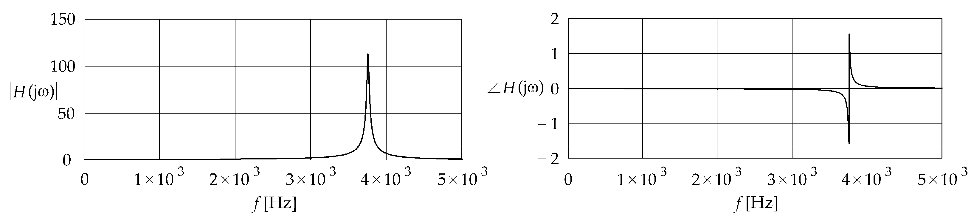
Figure 1 shows the amplitude and phase responses for the RLC interface of the AC traction network–pantograph given in Equations (8) and (9).

The frequency responses shown in Figure 1 confirm that the AC traction network–pantograph system exhibits a low-pass characteristic. It can be seen that low frequencies are faithfully transmitted, whereas higher frequencies are attenuated, reflecting the network’s ability to filter rapid voltage variations. A slight resonance peak appears near the natural frequency, the magnitude of which is limited by resistive damping.

In this work, the term higher harmonics refers to frequency components above the fundamental 50 Hz supply frequency, typically generated by traction converters, with significant contributions observed in the 250–3000 Hz range, as reported in measurement-based studies of AC railway systems.

The impulse response $h_{\mathrm{e}}\left(t\right)$ given in Equation (14) and associated with the transfer function $H_{\mathrm{e}}\left(\mathrm{s}\right)$ given in Equation (11) is:

$$h_e\left(t\right)=-{\displaystyle \frac{1}{LC{\omega }_{\mathrm{d}}}}{\mathrm{e}}^{-\zeta {\omega }_{\mathrm{n}}t}\mathrm{s}\mathrm{i}\mathrm{n}\left({\omega }_{\mathrm{d}}t\right),t>0$$

(37)

where ${\omega }_{\mathrm{d}}={\omega }_{\mathrm{n}}\sqrt{1-{\zeta }^2}$.

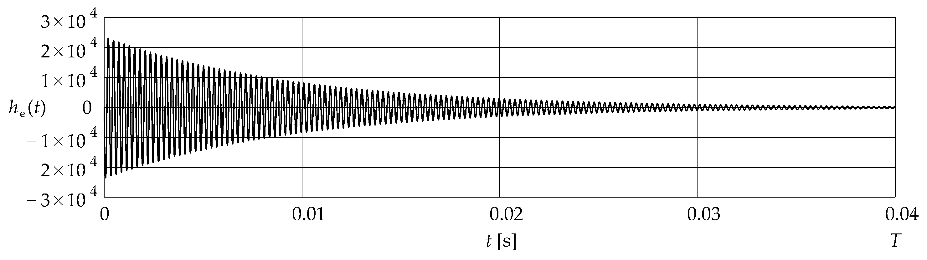
Figure 2 shows the impulse response $h_{\mathrm{e}}\left(t\right)$ given in Equation (37).

The impulse response shown in Figure 2 represents a typical second-order underdamped system behavior. A short pulse excitation produces an oscillatory waveform with decreasing amplitude, indicating the presence of inductive, capacitive, and resistive elements in the system. The rapid decay of the amplitude over time indicates the system’s stability and its effectiveness in suppressing disturbances after excitation. This behavior confirms that the analyzed traction system can be modeled as a damped RLC resonant circuit, in which the excitation energy is successively dissipated in the line resistance.

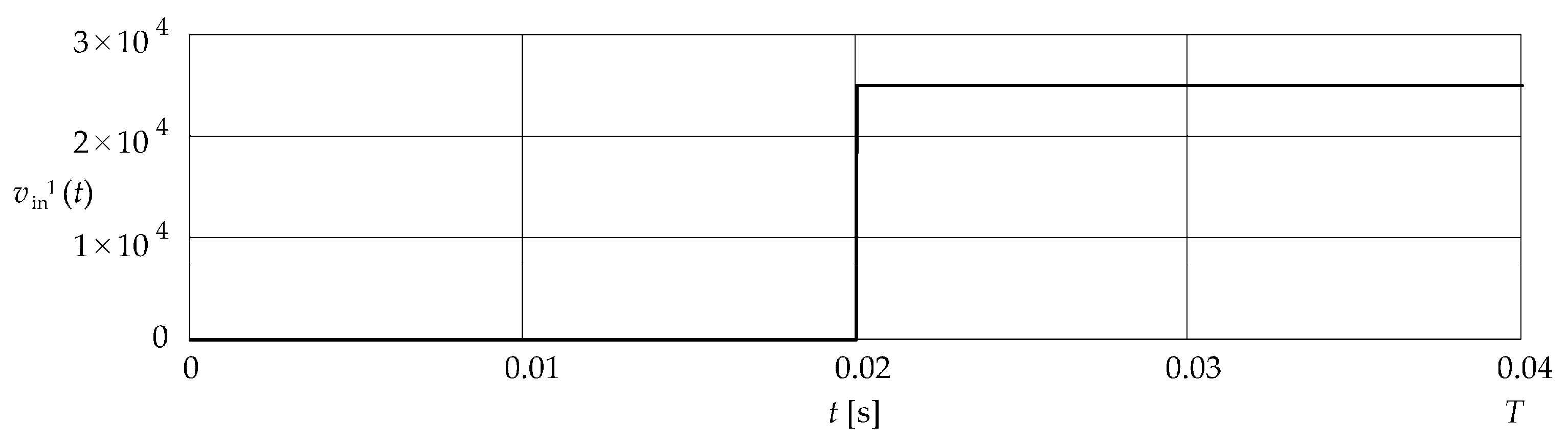
Figure 3 shows the unit step voltage excitation signal ${v_{\mathrm{i}\mathrm{n}}}^1\left(t\right)$ given in Equation (15) for the voltage $V_0$ equal to 25 kV.

The waveform shown in Figure 3 represents an abrupt increase in the supply voltage, used to evaluate the transient properties of the traction network–pantograph system. Such a signal allows the observation of how the pantograph voltage follows a sudden change in the input, revealing the system’s dynamic response characteristics.

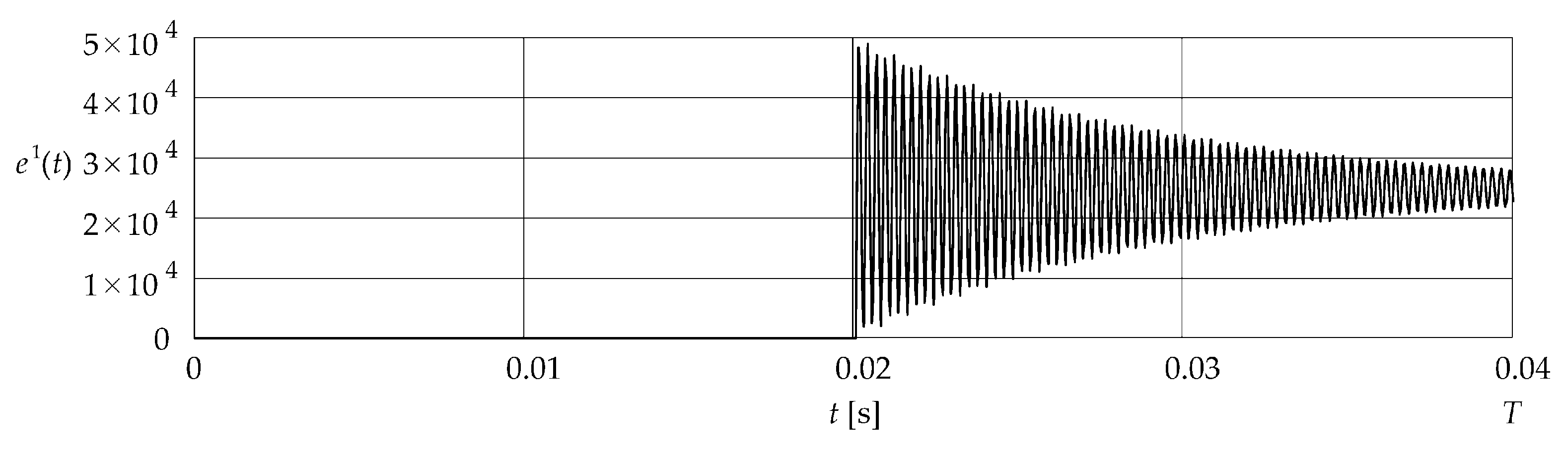
Figure 4 shows the error $e^1\left(t\right)$ given in Equation (13). Although true step-like changes rarely occur in real traction networks, the step excitation is retained in this work as a canonical signal for evaluating transient behavior. It enables the identification of fundamental dynamic characteristics such as rise time, overshoot and damping, which are directly related to the underlying RLC structure and resonance properties of the line. This type of excitation is widely used in dynamic system analysis because it reveals intrinsic properties of the system independently of specific operational scenarios.

In Figure 4, immediately after the step excitation, an oscillatory transient response appears, with amplitude gradually decreasing over time. The analyzed system behavior is characteristic of a damped RLC resonant circuit, in which the voltage deviation decays as energy is dissipated in the resistive elements of the network. The observed signal waveform confirms the system’s stability and its ability to effectively suppress transient disturbances following sudden voltage changes. The root mean square value of the dynamic voltage error ${e_{\mathrm{r}\mathrm{m}\mathrm{s}}}^1$ defined in Equation (19) is equal to $1.87\times {10}^4$ $\mathrm{V}$.

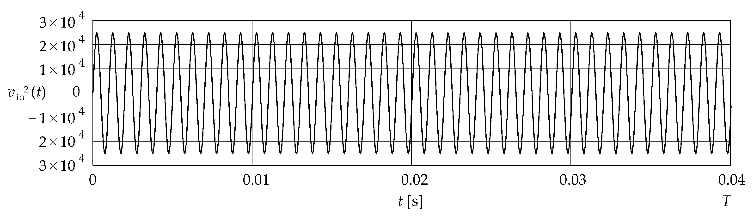
Figure 5 shows the sinusoidal voltage signal ${v_{\mathrm{i}\mathrm{n}}}^2\left(t\right)$ given in Equation (17) for the voltage $V_0$ equal to 25 kV.

The signal shown in Figure 5 is a pure sine wave with the amplitude of $V_0=25\mathrm{k}\mathrm{V}$ and the frequency $f$ of $1\mathrm{k}\mathrm{H}\mathrm{z}$. The waveform is periodic and symmetrical about the time axis, indicating the absence of a DC component. The period signal is $T=1\mathrm{m}\mathrm{s}$. The voltage varies smoothly from ${+V}_0$ and ${-V}_0$ without visible distortion or modulation.

The choice of a 1 kHz excitation signal in the sinusoidal test case is motivated by the characteristic spectral content of disturbances commonly observed in 25 kV AC traction systems. Measurements reported in the literature—including harmonic spectra of pantograph voltages and converter-induced emissions—indicate that onboard power-electronic converters generate significant harmonic components in the range of several hundred hertz up to approximately 2–3 kHz, with the 15th–25th harmonics of the 50 Hz fundamental often exhibiting the largest amplitudes. Furthermore, pantograph–catenary interaction phenomena such as contact fluctuations and arcing produce broadband components extending into the low-kilohertz region. The natural resonant frequencies of typical lumped-parameter equivalents of 25 kV lines also fall between roughly 700 Hz and 1.5 kHz, depending on line geometry and operating conditions. Consequently, an excitation at 1 kHz probes the system within a frequency region where both converter-related harmonics and resonance-driven amplification mechanisms are active. It therefore constitutes a representative and physically justified test signal for evaluating dynamic voltage deviations in the traction network–pantograph interface and aligns with the dominant disturbance mechanisms observed in measured pantograph voltage waveforms.

The excitation signals used in this study reflect the dominant spectral components and transient phenomena observed in real pantograph voltages of 25 kV AC traction systems. Field measurements reported in the literature show that onboard traction converters generate characteristic harmonic emissions extending from several hundred hertz to the low-kilohertz range, typically with prominent components around the 15th–25th harmonics of the 50 Hz supply. Furthermore, the pantograph–catenary interface is known to exhibit transient voltage perturbations caused by mechanical contact irregularities and intermittent arcing, whose spectra span a broad frequency band and often display significant energy in the 0.5–5 kHz region. These mechanisms combine with the natural resonant behavior of the line–pantograph system—whose dominant mode for typical 25 kV overhead lines lies between approximately 700 Hz and 1.5 kHz—to produce voltage distortions that closely resemble the bandwidth and structure of the test signals applied in this work. The sinusoidal excitation at 1 kHz therefore corresponds to a representative harmonic component within this resonance-enhanced range, while the multiharmonic and UBDE-derived waveforms emulate the composite and broadband disturbances characteristic of converter emissions, arcing events, and fast load variations. Consequently, the selected excitation signals provide a physically plausible and empirically grounded basis for evaluating the dynamic error behavior of the traction network–pantograph interface.

Although the lumped RLC model does not explicitly simulate the arc plasma dynamics or traveling-wave transients, the multi-harmonic and UBDE-derived excitation signals effectively reproduce the spectral signatures and broadband characteristics associated with arcing, impulsive overvoltage’s and converter-generated high-frequency components.

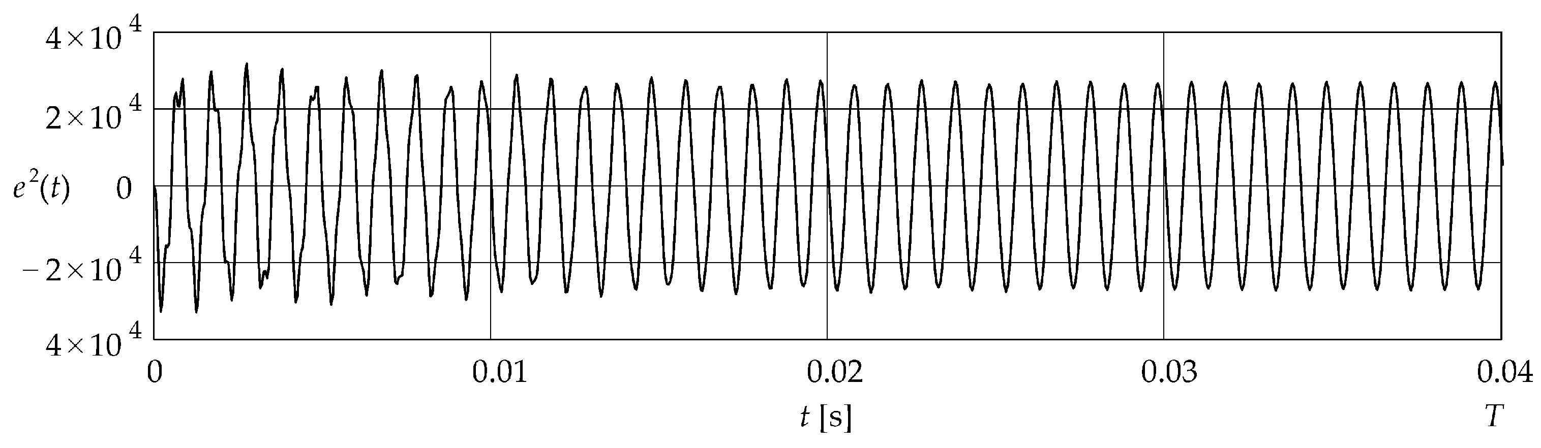
Figure 6 shows the error $e^2\left(t\right)$ given in Equation (13).

The analyzed signal is sinusoidal with an amplitude of $25\mathrm{k}\mathrm{V}$ and a frequency close to 1 kHz, corresponding to the input signal frequency ${v_{\mathrm{i}\mathrm{n}}}^2\left(t\right)$. The waveform is symmetric with respect to the time axis, confirming the absence of a DC component. Small amplitude fluctuations may result from system nonlinearity or transient effects. The signal remains periodic and stable over time. The root mean square value of the dynamic error ${e_{\mathrm{r}\mathrm{m}\mathrm{s}}}^2$ is equal to $1.91\times {10}^4$ $\mathrm{V}$.

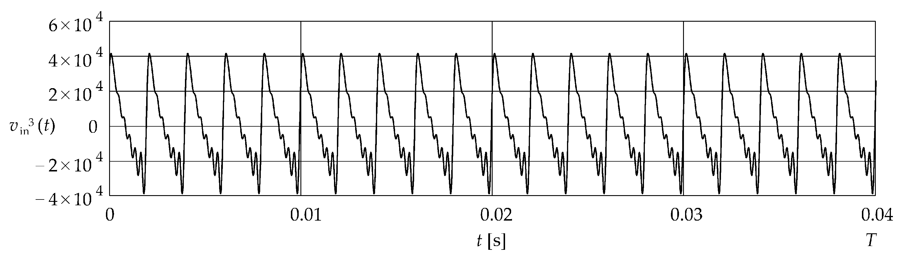
Figure 7 shows the multi-harmonic voltage signal ${v_{\mathrm{i}\mathrm{n}}}^3\left(t\right)$ given in Equation (18), for the parameter $N$ equal to 7. The corresponding voltage components $V_k,$ angular frequencies ${\omega }_k$ and initial phases ${\varphi }_k$ are equal to: ${\displaystyle \frac{V_0}{k}}$, $2\times \mathsf{\pi }\times k\times f_0$ and ${\displaystyle \frac{\mathsf{\pi }}{N-(k-1)}}$, respectively.

The waveform ${v_{\mathrm{i}\mathrm{n}}}^3\left(t\right)$ is non-sinusoidal and asymmetric, resulting from the superposition of seven harmonics ${(V}_0/k,{\omega }_k=2\mathsf{\pi }k{f}_0)$. Visible peaks and sharp transitions indicate the presence of higher-order harmonics. The signal is quasi-periodic, similar to a saw tooth wave, reflecting the nonlinear nature of the voltage and the richness of its spectrum.

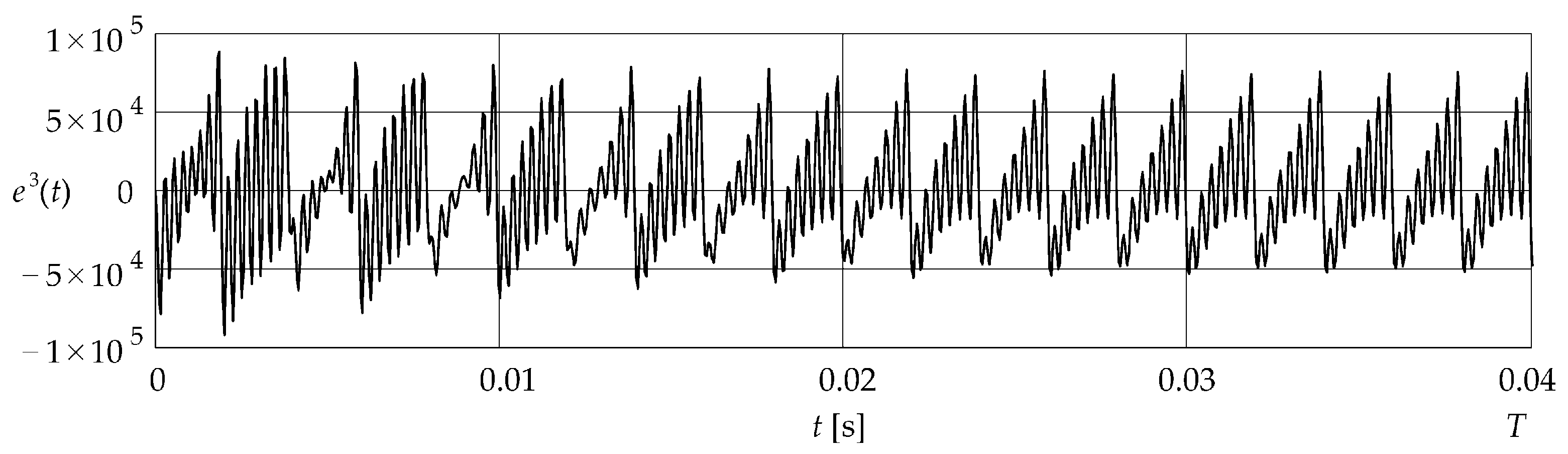
Figure 8 shows the error $e^3\left(t\right)$ given in Equation (13).

The signal $e^3\left(t\right)$ is clearly non-sinusoidal and exhibits strong fluctuations with a quasi-periodic structure. The presence of multiple frequency components leads to irregular oscillations and rapidly changing amplitude peaks. The analyzed signal revealed the presence of distorted harmonics, which manifests itself as the appearance of ${v_{\mathrm{i}\mathrm{n}}}^3\left(t\right)$ when applying. A dangerous amplitude envelope indicates nonlinear supply between harmonic components and possible phase differences between them. The calculated root mean square ${e_{\mathrm{r}\mathrm{m}\mathrm{s}}}^3$ is $3.36\times {10}^4$ $\mathrm{V}$.

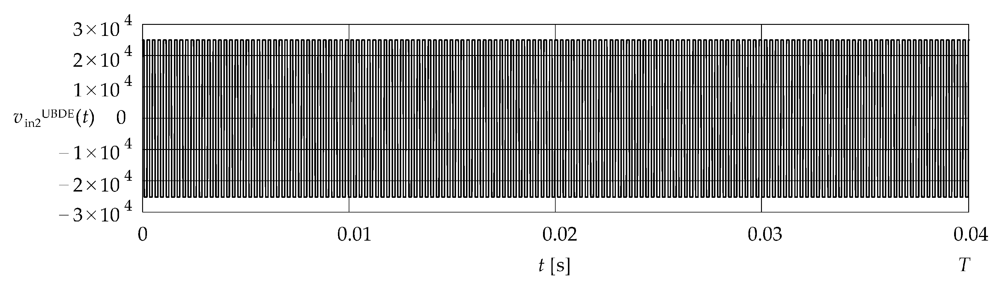
Figure 9 shows the signal ${v_{\mathrm{i}\mathrm{n}2}}^{\mathrm{U}\mathrm{B}\mathrm{D}\mathrm{E}}\left(t\right)$ with two constraints, obtained using the procedure defined in Equation (28) for $A=V_0$ and $L=50$.

The waveform shown in Figure 9 is constrained in both magnitude and duration, exhibiting a rectangular-like structure with 300 distinct switching events. The dense distribution of polarity reversals results from the iterative optimization process aimed at maximizing the mean-squared dynamic error under dual constraints. Such a waveform represents an adverse excitation scenario for the traction network–pantograph system, as the frequent switching efficiently excites the system’s resonant modes and amplifies its dynamic response. It constitutes the worst-case excitation scenario with two constraints, maximizing the root mean square value of the dynamic voltage error.

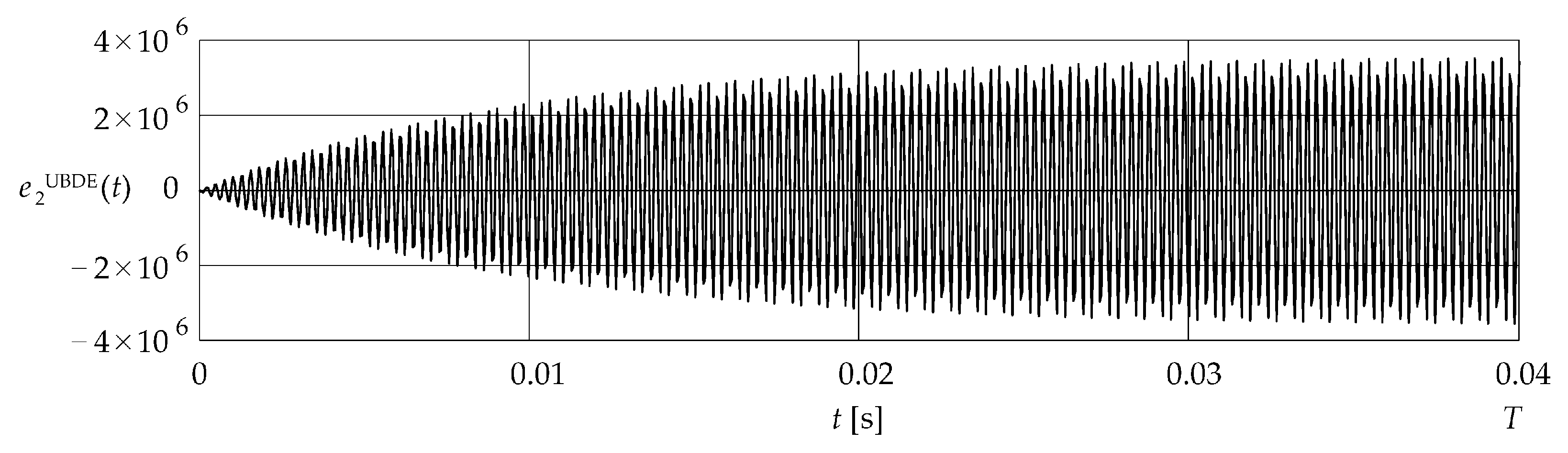
Figure 10 shows the error ${e_2}^{\mathrm{U}\mathrm{B}\mathrm{D}\mathrm{E}}\left(t\right)$ calculated using the formula given in Equation (28). This error represents the system’s response to the excitation signal ${v_{\mathrm{i}\mathrm{n}2}}^{\mathrm{U}\mathrm{B}\mathrm{D}\mathrm{E}}\left(t\right)$.

The error ${e_2}^{\mathrm{U}\mathrm{B}\mathrm{D}\mathrm{E}}\left(t\right)$ shows in Figure 10 exhibits an oscillatory character with a gradually increasing amplitude envelope, reaching its maximum near the end of the observation interval. The presence of high-frequency components and amplitude modulation indicates the excitation of resonant modes within the RLC traction network–pantograph interface. The error remains symmetric with respect to the time axis, confirming the absence of any DC component. The increasing oscillation amplitude reflects the accumulation of dynamic energy in the system under the excitation with 300 switching events. This signal represents the worst-case dynamic deviation achievable for dual-constrained excitation and corresponds to the maximum root mean square value of the dynamic voltage error. The root mean square value of the dynamic error ${e_2}^{\mathrm{U}\mathrm{B}\mathrm{D}\mathrm{E}}$ is equal to $4.12\times {10}^5$ $\mathrm{V}{\mathrm{s}}^2$. Considering that this error corresponds to the worst-case excitation scenario with two constraints, its value is several times higher than the root mean square error obtained for the three previously analyzed test-signal cases.

Although the signal shown in Figure 9 defines a theoretical upper bound for the excitation under dual constraints, its instantaneous vertical transitions make it difficult, or even impossible, to reproduce under real operating conditions. In practice, no physical system—including the AC traction network–pantograph interface—can generate such abrupt voltage changes due to its inherent inductive and capacitive dynamics. Therefore, to relate the constrained signal to realistic operation, an additional, third constraint must be introduced, limiting the rate of change in the signal. Under this additional limitation, the excitation waveform assumes a triangular or trapezoidal shape, depending on the switching instants. However, such a waveform cannot be determined analytically or through simple iterative methods because the problem becomes nonlinear and multimodal, involving an infinite number of admissible switching configurations [28,49].

To solve this problem and determine the worst-case excitation satisfying all three constraints: magnitude, duration, and rate of change, a Genetic Algorithm (GA) was employed. The GA was chosen for its proven capability to handle non-convex optimization problems and to explore complex search spaces where analytical gradients are unavailable. Each candidate solution (individual) represented a discretized voltage waveform ${v_{\mathrm{i}\mathrm{n}3}}^{\mathrm{U}\mathrm{B}\mathrm{D}\mathrm{E}}\left(t\right),$ expressed as a sequence of voltage samples constrained by both magnitude and slope constraints. The fitness function was defined as the mean-squared dynamic voltage error, calculated according to Equation (27), which served as the optimization criterion to be maximized. The initial population consisted of 50 individuals, randomly generated within the admissible solution space, ensuring that all initial candidates already satisfied the imposed physical constraints. The optimization process was carried out for 200 generations, with the crossover probability $p_{\mathrm{c}}=0.8$ and mutation probability $p_{\mathrm{m}}=0.05$. Selection was performed using the proportional reproduction method, favoring individuals with higher error energy, while offspring were generated using a single-point crossover operator. A random mutation operator was subsequently applied to maintain population diversity and to prevent premature convergence [28,49]. After each generation, a repair mechanism enforced the admissibility of solutions by projecting infeasible individuals back into the feasible region defined by Equations (32)–(35). To preserve progress across generations, the algorithm incorporated elitism, ensuring that the best individual, corresponding to the highest fitness value, was always retained. The optimization terminated when the fitness value reached convergence or after completing the maximum number of generations. The resulting excitation signal represents the worst-case, physically feasible waveform that maximizes the root mean square dynamic voltage error under triple constraints. From a physical perspective, this optimal excitation exhibits alternating triangular or trapezoidal segments, whose slopes are constrained by the rate of change constraint and whose polarity reversals efficiently excite the resonance modes of the RLC traction network–pantograph interface. Consequently, it defines the realistic upper bound on the dynamic voltage error energy, providing a rigorous and physically consistent methodology for evaluating the robustness of AC traction systems under dynamically feasible disturbances. The value of the rate of change constraint ($S_{\mathrm{m}\mathrm{a}\mathrm{x}}$), determined based on Equation (31), is: $2.31\times {10}^4$ V.

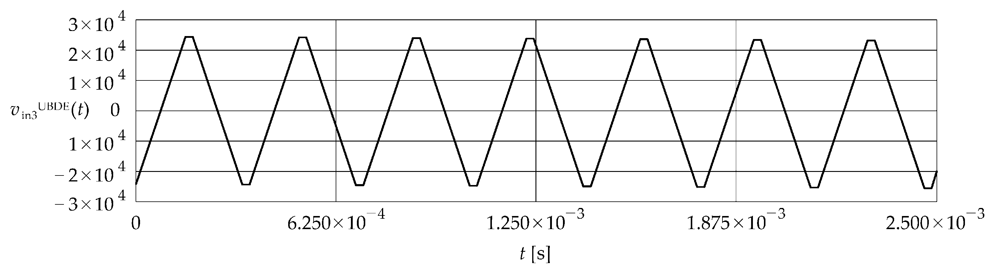
The excitation signal with three constraints, determined using the GA, contains more than 200 switching events. For better visualization of its waveform, only a fragment of the signal up to time $t=0.0025\mathrm{s}$ is presented in Figure 11.

The fragment of the signal ${v_{\mathrm{i}\mathrm{n}3}}^{\mathrm{U}\mathrm{B}\mathrm{D}\mathrm{E}}\left(t\right)$ presented in Figure 11 exhibits a purely trapezoidal waveform composed of 15 rising and falling slopes. The switching instants are symmetrically distributed within the analyzed time window, resulting in a balanced excitation pattern that satisfies all three imposed constraints, including the rate of change constraint.

The error ${e_3}^{\mathrm{U}\mathrm{B}\mathrm{D}\mathrm{E}}\left(t\right)$ exhibits a waveform very similar to that shown in Figure 10; however, it demonstrates a lower magnitude, ranging from approximately $-2.4\times {10}^6 \mathrm{V}$ to $2.4\times {10}^6\mathrm{V}$. The root mean square value of the dynamic error ${e_3}^{\mathrm{U}\mathrm{B}\mathrm{D}\mathrm{E}}$ is equal to $3.02\times {10}^5$ $\mathrm{V}{\mathrm{s}}^2,$ which corresponds to about 73% of the corresponding error value obtained in response to the excitation signal with two constraints. The lower value of the error ${e_3}^{\mathrm{U}\mathrm{B}\mathrm{D}\mathrm{E}}$ compared to ${e_2}^{\mathrm{U}\mathrm{B}\mathrm{D}\mathrm{E}}$ results from the imposition of the third constraint (rate of change) on the excitation signal.

To assess the robustness of the optimization procedure, the evolution of the objective function value across generations was analyzed for the UBDE search. The resulting convergence curve shows a rapid initial decrease in the fitness function during the first several dozen generations, followed by a gradual flattening as the population approaches the neighborhood of the global optimum. After approximately 120–150 generations, the improvements become marginal, indicating that the algorithm has effectively converged and that further iterations yield no significant reduction in the dynamic error bound. This behavior is consistent with typical GA dynamics and demonstrates that the adopted population size and genetic operators ensure stable and reproducible convergence for the class of excitation signals considered in this study. The curve also confirms that the UBDE result reported in the paper is not a numerical artifact but the outcome of a well-behaved optimization process.

3.1. Validation and Practical Interpretation of the Results

Although the present study is based on analytical modeling and simulation, the obtained dynamic error values can be meaningfully interpreted in the context of real pantograph voltage measurements available in the literature. An important empirical reference is the dataset published by Mariscotti (2020)—Ref. [9], which contains more than 21,000 short recordings of pantograph voltage and current collected on several European AC railway systems, including two 25 kV/50 Hz lines that correspond to the type of traction network analyzed in this work.

Inspection of the waveforms and spectra shown in the dataset indicates that pantograph voltages exhibit distortions and transient fluctuations that frequently reach several hundred volts. For example, the typical 25 kV waveforms reported for the Italian and French 50 Hz systems show noticeable deformation of the voltage peaks, while the corresponding spectra reveal harmonic content extending to several kilohertz. Such deviations are consistent with the combined effects of converter emissions, mechanical contact variations, resonance interactions, and line impedance variability described by the author. These empirical observations imply that short-term voltage deviations in the range of 0.5–3% of the nominal 25 kV voltage—corresponding to approximately 125–750 V—occur routinely under normal operating conditions, and may temporarily exceed these values during dynamic events such as arcing or rapid load transitions.

When viewed against this background, the dynamic error values obtained in the present study fall within a realistic and physically meaningful range. The RMS dynamic error computed for the sinusoidal excitation is of the order of a few hundred volts, which corresponds to a deviation of roughly 1% of the nominal line voltage. This is consistent with the typical harmonic-related distortions observable in the 25 kV measurement data. The RMS error obtained for a multi-harmonic excitation is higher and reaches approximately 2% of the nominal voltage, which remains well aligned with deviations visible in the empirical waveforms during high-load traction or regenerative braking periods. These values reflect disturbances that are not only theoretically plausible but also commonly observed in practice.

The largest dynamic errors in this work arise under the UBDE excitation, which represents a worst-case, yet physically admissible, signal. The corresponding RMS error is on the order of 4% of 25 kV. Although this level of deviation is at the upper end of what is typically observed, it remains compatible with the empirical evidence. The Mariscotti dataset includes recordings where voltage distortions and transient peaks exceed several percent of the nominal value, especially during operating states where harmonic distortion, contact mechanics, and line impedance interactions combine to amplify deviation. Thus, the UBDE-based dynamic error should be interpreted as an upper bound on disturbances that remain feasible under real operating conditions.

A further reduction in the error is obtained when the physically justified rate-of-change constraint is included. This constraint reflects the finite ability of the traction line to follow abrupt changes in excitation and yields dynamic error values of approximately 1.5% of nominal voltage. This level corresponds closely to the range of disturbances observed in the field recordings after filtering based on EN 50163 criteria, as performed by Mariscotti when preparing the dataset. The agreement indicates that once realistic physical limits are applied, the UBDE framework predicts error levels that fall comfortably within known operational behavior.

Expressing the results in percentage form also enables a meaningful comparison with the voltage deviation limits defined in standards such as EN 50163 and IEC 60850. These documents allow short-duration voltage variations that can deviate from the nominal value by several percent without violating long-term operational limits. The dynamic error levels obtained in this study lie within or close to these tolerances, indicating that the proposed UBDE-based method is suitable for assessing compliance margins and robustness in traction power systems.

In summary, the qualitative agreement between the simulated dynamic error values and the disturbance levels observed in the measured pantograph voltage data confirms the practical relevance of the proposed approach. Although direct numerical matching between the UBDE results and specific empirical snippets is beyond the scope of this work, the percentage-based comparison provides a robust form of validation. It demonstrates that the UBDE framework produces realistic, physically grounded estimates of worst-case dynamic behavior and can therefore be used as a meaningful tool for voltage-quality assessment, system design, and dynamic performance analysis in AC traction power networks.

A practical interpretation of the obtained results can be made by relating the UBDE value to the voltage deviation limits defined in EN 50163. For a nominal voltage of 25 kV, the standard allows short-duration deviations of up to approximately $\pm 5\%$ under normal operating conditions. For illustration, consider a UBDE value of 480 V obtained for the physically constrained excitation. This corresponds to a relative deviation of $480 \mathrm{V}/\mathrm{25,000} \mathrm{V}\approx 1.9\%$. Such a deviation remains well within the short-term limits permitted by EN 50163, indicating that even in the worst-case dynamically feasible scenario, the traction network–pantograph interface does not exceed the permissible voltage envelope. This example demonstrates how the UBDE metric can be used to assess the compliance margin of a traction system and to determine whether its dynamic behavior remains compatible with standardized performance requirements.

3.2. Practical Applications of the UBDE Methodology

The UBDE framework proposed in this study offers several practical applications for AC traction power systems, complementing classical power quality indicators and providing a new perspective on the dynamic behavior of the pantograph–network interface. Its ability to quantify the worst-case dynamic voltage deviation under physically feasible excitations makes it particularly useful for railway infrastructure managers, rolling stock manufacturers, and system designers.

First, UBDE can support the design and tuning of passive and active filtering devices, such as LCL filters, damping networks, or harmonic compensators used on-board or within substations. By identifying excitation patterns that maximize dynamic error, the method highlights the frequency ranges and transient characteristics most critical for voltage stability, allowing targeted filter optimization rather than relying solely on steady-state harmonic analysis.

Second, UBDE provides a tool for specifying voltage quality requirements for both infrastructure and rolling stock. Conventional standards such as EN 50163 and IEC 60850 define admissible long-term voltage envelopes but do not give explicit limits for the maximum dynamic deviation during short transient events. The UBDE-derived dynamic accuracy class proposed in this work can be used to complement existing regulations by offering a quantifiable, physically grounded measure of the network’s voltage-following capability.

Third, the method can be applied in robustness and sensitivity studies of traction supply systems. The UBDE-based dynamic error reveals how the pantograph voltage responds to worst-case disturbances occurring within a defined range of magnitudes, rates of change, or durations. This makes it possible to assess the resilience of the system to fast-changing loads, converter emissions, or mechanical irregularities such as contact losses or short arcing intervals.

Fourth, the methodology has potential for diagnostic and monitoring applications. A comparison between measured pantograph voltages and UBDE-based predictions may help in detecting abnormal operating conditions, such as degraded overhead contact line impedance, aging of filtering components, or malfunctioning converters whose emissions exceed physically expected limits. In this sense, UBDE can serve as a reference for identifying deviations that cannot be explained by normal dynamic behavior.

Finally, the proposed approach can provide simulation-based support for planning and upgrading traction networks. Since UBDE quantifies the maximum deviation between feeder and pantograph voltages, it can be used to evaluate how changes in line parameters, reinforcement strategies, resonance mitigation measures, or increased traffic intensity influence the dynamic performance of the system. This may assist infrastructure managers in prioritizing investments and ensuring compliance with voltage-quality requirements under future loading conditions.

Overall, the UBDE methodology offers a set of practical tools for improving the design, operation, and assessment of AC traction power systems. By integrating dynamic performance considerations with physically feasible constraints, it enables a more comprehensive evaluation of voltage quality than is possible with conventional steady-state or harmonic-based methods alone.

The concept of dynamic accuracy class introduced in this study refers to a quantitative measure of how well the traction network–pantograph system is able to reproduce the feeder voltage under realistically varying operating conditions. It represents the maximum voltage deviation that may occur in response to all physically admissible disturbances, taking into account limits on the magnitude, duration and rate of change in the excitation. As such, it provides a worst-case, time-domain complement to traditional power-quality indicators such as harmonic distortion or flicker, which describe only steady-state or periodic disturbances. The dynamic accuracy class, therefore, offers a practical and comprehensive way to characterize the system’s robustness to fast, broadband or transient effects that are typical in railway operation and are not captured by conventional metrics. Thus, the UBDE-derived performance limits provide directly actionable information for filter design, protection coordination and assessing the robustness of rolling stock and infrastructure to the fastest physically admissible disturbances.

4. Conclusions

This article presented a comprehensive methodology for assessing the dynamic accuracy of the AC traction network–pantograph interface modeled as an equivalent RLC circuit derived from a distributed-parameter system. The proposed approach combines analytical, numerical, and optimization-based approaches to determine the dynamic voltage error generated in response to various excitation conditions. The test results confirmed that the analyzed system acted as a low-pass filter. It accurately reproduced low-frequency voltage changes while simultaneously attenuating higher-frequency signals. A small dynamic voltage error was observed for sinusoidal and multiharmonic excitations, which increased only slightly with increasing harmonic number and frequency. For the dual-constrained excitation ${v_{\mathrm{i}\mathrm{n}2}}^{\mathrm{U}\mathrm{B}\mathrm{D}\mathrm{E}}\left(t\right),$ the highest dynamic error was obtained, with a root mean square (RMS) value of approximately $4.10\times {10}^5$ $\mathrm{V}$, corresponding to the worst-case response among all analyzed test signals. After imposing the third constraint—the rate of change constraint—the physically feasible excitation ${v_{\mathrm{i}\mathrm{n}3}}^{\mathrm{U}\mathrm{B}\mathrm{D}\mathrm{E}}\left(t\right)$ generated a lower RMS error of $3.02\times {10}^5$ $\mathrm{V},$ which represents about 73% of the dual-constrained case. This reduction clearly demonstrates the influence of the slope constraint in suppressing high-frequency oscillations and improving system stability. The use of the Genetic Algorithm (GA) to identify the worst-case excitation satisfying all three physical constraints proved to be an effective and versatile optimization tool. The GA allowed the generation of excitation waveforms and corresponding dynamic errors that most accurately reflect real operating conditions. Consequently, the obtained results can be interpreted as an equivalent dynamic accuracy class, defining the system’s ability to reproduce voltage variations within physically admissible limits. The proposed UBDE-based methodology provides a quantitative approach for evaluating the dynamic accuracy and robustness of traction power supply systems. Future research will focus on extending the interface modeling to include nonlinear and distributed effects, as well as on determining dynamic errors for other classes of test signals and alternative dynamic error functions, which will enhance the universality and practical applicability of the developed approach.