1. Introduction
Driven by the dual carbon goals of carbon peak and carbon neutrality, building a new power system dominated by renewable energy has become the developmental target and new form for the future energy and power sector. When high-penetration renewable energy is integrated into the distribution network in a distributed manner, the poor match between renewable energy output and user load profiles leads to intensified fluctuations in the net load curve on the lines during actual operation, exhibiting strong intermittency and uncertainty, which poses challenges to the flexibility of power system operation.
After connecting to the grid, user-side demand resources can provide diverse power services for the power system. Microgrids can aggregate different distributed resources to form a bidirectionally adjustable independent dispatch unit participating in the grid’s optimal dispatch calculation [
1]. During regulation, control of internal units typically aims to maximize renewable energy consumption and reduce system operating costs, among other objectives [
2]. Virtual Power Plants (VPPs) can coordinate the tensions between the grid and distributed generation, fully exploit the potential of distributed resources, and bring economic benefits to both the grid and users [
3]. By enhancing the overall benefits of the VPP itself and its members, the enthusiasm for renewable energy participation in the market is increased [
4].
Currently, domestic and international scholars have conducted extensive research on optimization operation technologies for user-side aggregators. Reference [
5] provides a detailed analysis of the demand response potential of air conditioning load clusters and their duration. Reference [
6] focuses on analyzing the energy system of building air conditioning systems, specifically discussing dynamic building air conditioning load calculation and the energy consumption calculation of air conditioning systems. Reference [
7] details an energy-saving optimization model for central air conditioning systems. Reference [
8] achieved a reduction in the deviation between actual load and transacted electricity, thus improving distribution network power balance issues, through optimal control of central air conditioning loads in large smart parks. Reference [
9] considered the impact of cycle throughput and depth of discharge on energy storage system life degradation. Reference [
10] studied the effects of operating temperature, charge/discharge power, and state of charge (SOC) on electrochemical energy storage systems. Reference [
11] considered the charging strategy of a public parking lot with a photovoltaic system, analyzing its environmental impact and economic benefits. Reference [
12] used minimizing power fluctuation on the distribution network tie-line side as the optimization objective for orderly power utilization management.
Reference [
13] constructed a day-ahead optimal operation model for a wind-PV-thermal combined generation system based on price-based demand response. Reference [
14] obtained user flexible load response strategies by adjusting peak-shaving compensation prices, achieving maximum benefits for both through a Stackelberg game. Reference [
15] established a day-ahead joint clearing model for the energy and ancillary services market based on flexibility enhancement, effectively categorizing the performance differences in flexibility resources. A variety of optimization frameworks have been proposed for distribution network-aggregator coordination, yet most are computationally intensive and require complete physical models. Data-driven methods offer a promising alternative, but their integration into multi-objective distribution network optimization remains underexplored.
Although progress has been made in load aggregator demand response, some issues remain unresolved. For instance, how to further improve decision-making efficiency and accuracy, and how to utilize historical data for clearing decisions under limited mechanistic model parameters. These problems require further research.
2. Optimal Operation Model of Distribution Networks
With the transformation of the energy structure in the new power system and the continuous development of electricity market reforms, the high-proportion integration of distributed renewable energy into distribution networks has become an inevitable trend. However, the output characteristics of high-penetration renewable energy and user load curves are often not fully complementary. Their integration into the distribution network can lead to increased fluctuations in the line net load, resulting in insufficient operational flexibility for the distribution network and its upstream grid.
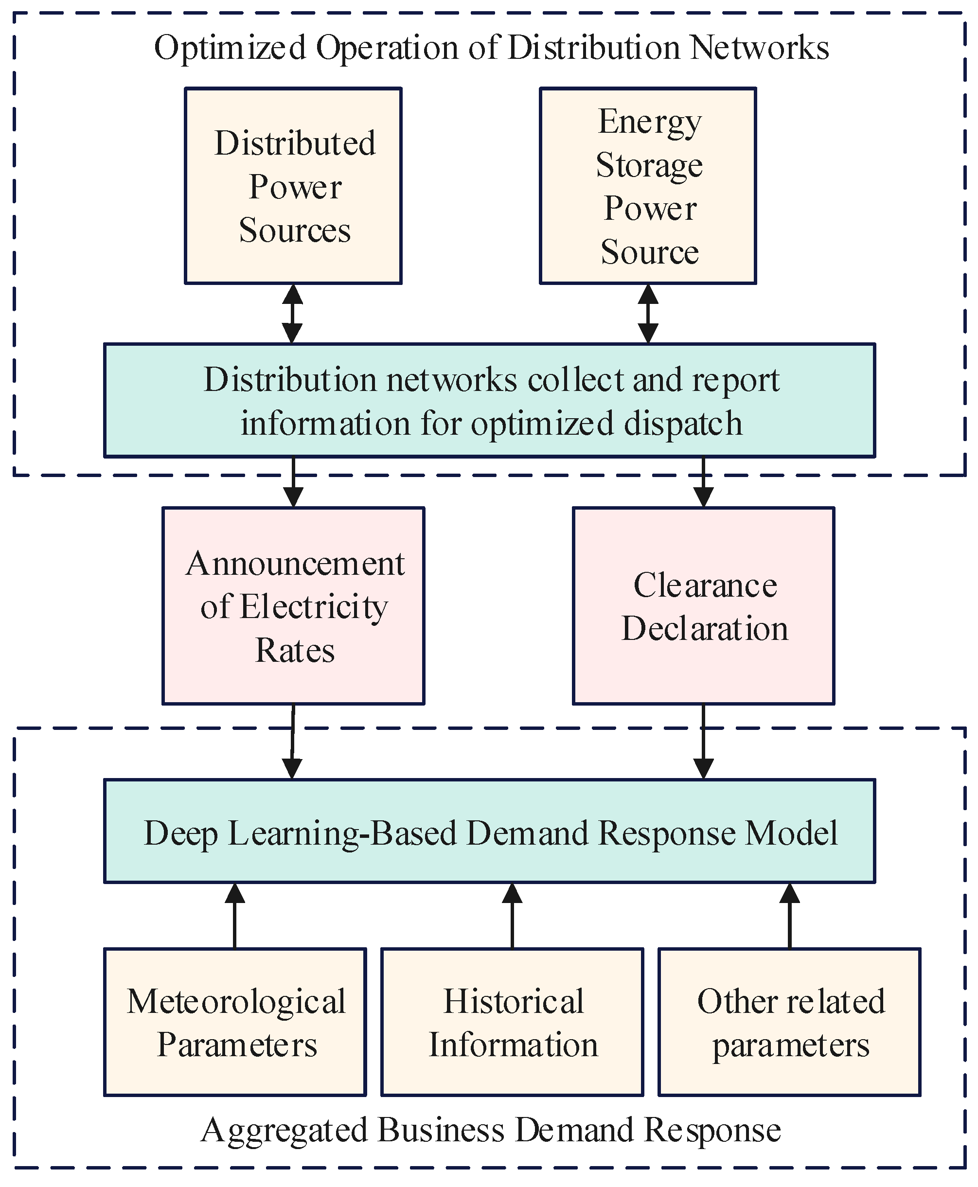
Under the ongoing development of the new power system, the flexible resources connected at the user side are also increasingly diverse. Traditional resources include residential and commercial air conditioning loads, adjustable commercial and industrial loads, and interruptible commercial and industrial loads. Emerging resources further include distributed renewable energy, energy storage, electric vehicles, and thermal storage/cooling equipment. On one hand, a large number of decentralized flexible resources are intricately distributed across various lines of the distribution network, increasing the difficulty for the DNO to dispatch and control them. On the other hand, with electricity market reforms, some distributed resources are built by users or independent suppliers; their ownership no longer belongs to the grid, forming independent entities that the DNO cannot dispatch uniformly. Therefore, this paper comprehensively considers the response and control characteristics of various schedulable resources on the user side. It directly manages grid-side DG and energy storage devices, while employing a TOU pricing mechanism to transact with extensive flexible resources for their tie-line power. The dispatch operation framework of a distribution network with aggregator participation is shown in
Figure 1. As the distribution network and aggregators belong to different interest entities, their dispatch objectives differ. Typically, aggregators have limited capacity and minimal impact on market prices; thus, they are considered price-takers, adjusting their response strategies based on the prices offered by the DNO. The DNO updates electricity prices according to the received operation strategies from aggregators and adjusts the operation modes of other controllable flexible resources to meet its own operational requirements.
2.1. Aggregator Demand Response Model
2.1.1. Introduction to the Deep Learning Model
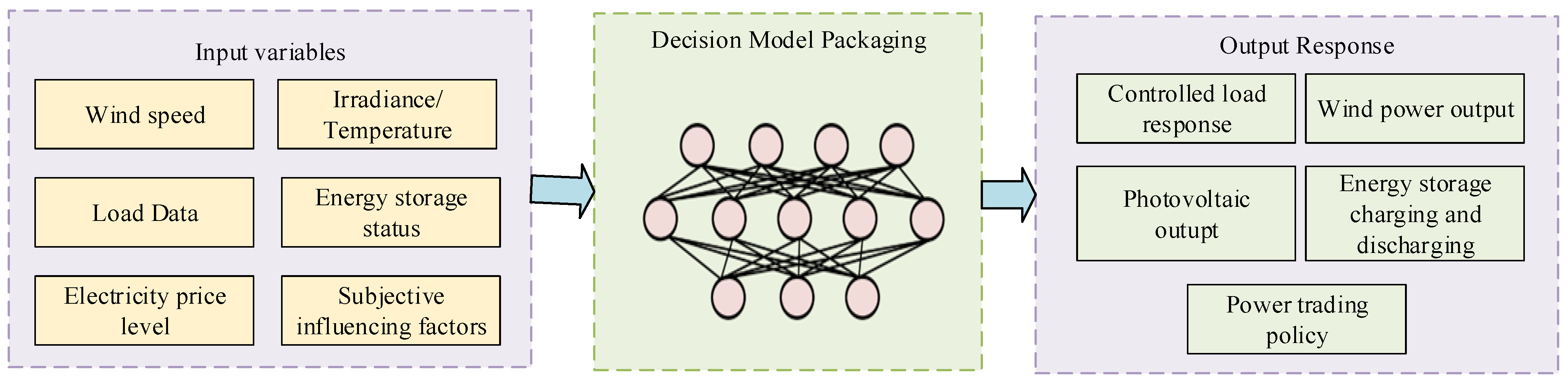
When an aggregator directly dispatches and controls its internal schedulable resources, the diversity of individual resources determines the complexity of its response model. The modeling and analysis process involving high-dimensional nonlinear superposition limits the aggregator’s ability to regulate and analyze the aggregated response of numerous flexible individuals. Therefore, this section adopts the deep learning-based intelligent decision-making demand response method for aggregators. Based on the structural and correlational characteristics of the responsive resources, it takes wind speed, solar irradiance, temperature, load, electricity price, and other related factors as input variables, and the demand response of flexible resources and the aggregator’s decision results as output variables. The aggregator decision framework for response output is shown in
Figure 2.
Aggregators can input day-ahead electricity price information released by the DNO, combined with historical operation data and meteorological information, into a pre-trained deep learning demand response decision model with optimal parameters. This enables accurate clearing strategies for electricity purchase and sale without needing to know detailed physical model parameters of users. After obtaining specific clearing data from each aggregator, the DNO, considering the actual network configuration, constructs a multi-objective optimal operation model that comprehensively considers operational costs and network flexibility requirements. It then optimizes electricity prices based on the operation results and disseminates the updated price information to aggregators. This iterative calculation process repeats until the final distribution network operation objectives converge, completing the two-layer dispatch operation process between the distribution network and aggregators.
2.1.2. Training Data Generation for the Deep Learning Model
The training dataset for the deep learning-based aggregator model is generated through systematic simulation of the aggregator’s optimization behavior under diverse operating scenarios. This approach addresses the challenge of insufficient historical operational data in emerging flexibility markets while ensuring comprehensive coverage of possible operating conditions.
Specifically, the training samples are generated by solving the aggregator’s cost minimization problem under various combinations of input parameters:
- (1)
Electricity price profiles: Time-of-use pricing schemes with peak prices ranging from 0.8 to 1.2 yuan/kWh, valley prices from 0.3 to 0.5 yuan/kWh, and flat prices from 0.5 to 0.7 yuan/kWh. Different peak-valley time arrangements are considered to reflect diverse pricing strategies.
- (2)
Renewable energy generation: Wind and photovoltaic output profiles based on historical meteorological data, covering different seasons and weather conditions. Wind speeds range from 3 to 15 m/s, and solar irradiance varies from 0 to 1000 W/m2.
- (3)
Temperature conditions: Outdoor temperature profiles ranging from 15 °C to 35 °C, which significantly affect air conditioning load behavior and user comfort requirements.
- (4)
Initial system states: Energy storage state-of-charge (SOC) values uniformly distributed between 20% and 80%, and initial indoor temperatures for air conditioning loads ranging from 22 °C to 28 °C.
- (5)
Subjective constraint parameters: User comfort preferences including maximum allowable temperature deviations (±2 °C to ±4 °C), maximum number of air conditioning adjustments per day (2 to 6 times), and energy storage cycling limits (1 to 3 cycles per day).
Through Latin hypercube sampling of the above parameter space, a total of 7000 training samples were generated. Each sample consists of:
- -
Input features (dimension: 168): 24 h electricity price signals, 24 h renewable generation forecasts, 24 h temperature forecasts, initial system states, and constraint parameters.
- -
Output labels (dimension: 72): 24 h power exchange schedule with DNO, 24 h energy storage charging/discharging power, and 24 h air conditioning load adjustment decisions.
The dataset was partitioned into a training set (4900 samples, 70%), validation set (1050 samples, 15%), and testing set (1050 samples, 15%). The training set is used for model parameter learning, the validation set for hyperparameter tuning and early stopping, and the testing set for final performance evaluation.
It should be emphasized that this deep learning model serves as a surrogate model for the aggregator’s optimization behavior. Once trained offline, it can rapidly predict the aggregator’s clearing strategy given new price signals and forecasts, without requiring access to detailed physical parameters of individual resources. This approach not only protects user privacy but also enables real-time decision-making in the upper-level distribution network optimization.
2.2. Distribution Network Operation Objectives and Constraint Functions
Distributed generation, energy storage batteries, and aggregators within the distribution network can all participate in distribution network operation as flexible dispatch resources. According to the individual characteristics of flexible resources, different methods are adopted for dispatch management. The distribution network can directly control DG and energy storage batteries. However, aggregators, as independent interest entities, cannot be directly controlled. Generally, the DNO can guide the response characteristics of aggregators by formulating incentive policies. This chapter primarily considers the DNO using a TOU pricing mechanism as an incentive for aggregators. Through day-ahead dispatch operation, while maintaining its own interests, the DNO needs to preserve the operational flexibility of the distribution network under high renewable energy penetration. That is, by dispatching flexible resources, it can rapidly respond to fluctuations in the distribution network’s net load power. Based on the aforementioned analysis, this section constructs a multi-objective optimization function that comprehensively considers the economic and flexibility requirements of distribution network operation.
2.2.1. Objective Functions
Economic Objective of Distribution Network Operation: The economic requirement considered in this paper is the minimization of the equivalent operational cost of the distribution network. The objective function is as follows:
In the formula, the numerator includes the electricity purchase cost from the upstream grid, the cost of purchasing electricity from DG, the dispatch cost of energy storage units, and the power loss cost. The denominator represents its revenue from energy sales, including the electricity sales revenue from the distribution network to aggregators and other load entities.
H is the number of time slots corresponding to one dispatch cycle;
N is the number of distribution network nodes;
is the electricity selling price from the distribution network to other load entities;
is the load power at node
i at time
t; C
LA is the revenue from electricity sales to aggregators; C
G is the cost of purchasing electricity from the upstream grid; C
DG is the cost of purchasing electricity from DG; C
ESS is the dispatch cost of energy storage units; C
LOSS is the active power loss cost of the distribution network.
where
is the electricity selling price from the DNO to aggregators; N
LA is the number of aggregators connected to the distribution network;
is the power purchased by the
i-th aggregator at time
t.
where
is the electricity purchase price from the upstream grid, determined and published by the upstream grid;
is the power purchased from the upstream grid at time
t.
where
is the electricity purchase price from the distribution network to grid-side DG; N
DG is the number of DG units connected to the distribution network;
is the output power of the
i-th renewable energy source at time
t.
where N
ESS is the number of energy storage devices;
γESS is the dispatch cost per unit power of the energy storage device;
and
are the charging and discharging power of the
i-th energy storage device at time t, respectively.
where
γG is the price corresponding to the active power loss of the distribution network, generally determined by the upstream grid electricity price;
M is the number of branches;
is the line loss of the
i-th branch at time
t.
Flexibility Objective of Distribution Network Operation: The net load of the distribution network includes the aggregation of loads, DG, and other flexible resources. Therefore, when there is a high proportion of renewable energy on the grid side, it may cause significant fluctuations in the net load at the distribution network side, reducing operational flexibility, greatly affecting the security and stable operation of the distribution network, and consequently weakening its accommodation capability for renewable energy. Thus, the distribution network’s accommodation level for the uncertain fluctuations of renewable energy can, to some extent, be understood as its operational flexibility adaptability.
The net load fluctuation rate is an important indicator reflecting the distribution network’s ability to accommodate renewable energy. For the distribution network, the fluctuation of tie-line power directly reflects the fluctuation degree of its actual load. This variable can be described as the rate of change in the distribution network’s net load per unit time, reflecting the fluctuation trend of the net load within a unit time. The specific expression for the distribution network net load fluctuation rate is:
where
is the net load fluctuation rate;
is the net load of the distribution network at time
t;
is the net load of the distribution network at time
t − 1. When the net load fluctuation rate is less than the maximum allowable fluctuation level for system operation, the system is considered to meet flexibility requirements; otherwise, it indicates insufficient system flexibility.
In this paper, to ensure the operational flexibility of the distribution network, minimizing the sum of absolute net load fluctuation rates is considered as an objective function, expressed as:
The net load fluctuation rate is selected as the primary flexibility indicator for the following reasons. First, under high renewable penetration, the key flexibility challenge is managing rapid net load variations; this rate directly quantifies that challenge. Second, as a continuous and differentiable function, it can be directly incorporated into the NSGA-II framework without complex scenario enumeration. Third, minimizing the net load fluctuation rate is positively correlated with improving upward and downward flexibility margins. Additional metrics (e.g., ramp capacity, reserve margins) could be added but would increase the dimensionality of the Pareto front; their integration is left for future research. The case study results (Scenario 3 vs. base case) show that the proposed framework improves net load adequacy while reducing the fluctuation rate, confirming its effectiveness in enhancing renewable accommodation.
A multi-objective optimization objective function for the distribution network is constructed by comprehensively considering the minimization of comprehensive operational costs and the net load fluctuation rate.
2.2.2. System Operation Constraints
Active and Reactive Power Balance Constraints:
where
is the reactive power from the transmission system at time
t;
is the reactive power at node
i at time
t;
is the reactive power of aggregator
i at time
t;
is the reactive power loss of branch
i at time
t.
where
is the voltage at node
i;
is the voltage at node
j;
and
are the conductance and susceptance between nodes
i and
j, respectively;
is the phase angle difference between nodes
i and
j.
Node Voltage Constraint:
where
and
are the minimum and maximum voltage magnitudes at the
i-th node, respectively.
Distributed Generation Constraint:
where
is the maximum output limit of the
i-th DG unit.
Gas Turbine Ramp-up and Ramp-down Constraints:
where
is the output power of the gas turbine at time t;
and
are the upper and lower limits for ramp-up and ramp-down rates of the gas turbine, respectively.
Energy Storage Constraints:
where
and
are the charging and discharging power of the energy storage at time t, respectively;
PCMAX and
PDMAX are the maximum charging and discharging power of the energy storage battery, respectively;
is the state of charge (SOC) of the energy storage battery at time
t;
δ is the self-discharge rate per unit time of the energy storage battery;
and
are the charging and discharging efficiencies of the energy storage battery, respectively; the energy storage battery needs to maintain its SOC within a stable range during normal operation, with
Smin and
Smax being the lower and upper limits of the SOC at time t, respectively.
Flexibility Constraint:
where
is the net load fluctuation rate of the distribution network at time
t;
is the maximum allowable value of the net load fluctuation rate at time
t.
3. Multi-Objective Optimization Solution Method
In traditional trading models, the DNO provides day-ahead trading price curves to each aggregator based on its operational requirements. Each aggregator then performs optimization calculations based on the given prices and its own demand objectives, feeding the optimized clearing results back to the DNO. This interactive process forms a leader-follower game-based electricity trading strategy, ultimately seeking a Nash equilibrium solution for both objectives. This chapter, however, forms an aggregated model for the aggregator’s clearing strategy through deep learning training, establishing a direct mapping between electricity prices and corresponding output strategies, thereby eliminating the need for dual iterative optimization. The DNO only needs to calculate its own objectives based on the aggregators’ clearing strategies. This approach, on one hand, allows aggregators to operate without needing users’ physical models, protecting user information privacy; on the other hand, it can improve the efficiency of solving the distribution network’s objective function and enhance system operational efficiency.
When performing optimal operation calculations, the distribution network considers multiple objectives, including operational cost and power fluctuation rate. Traditional methods for solving multi-objective problems often use weighting methods or distance function methods, which essentially convert multi-objectives into a single-objective function for solution. In cases where objective functions compete and constrain each other, making it difficult to assign reasonable weights, evolutionary algorithms based on the Pareto mechanism can be used to solve multi-objective functions directly without weighting the objectives. This chapter selects the fast non-dominated sorting genetic algorithm (NSGA-II) for multi-objective solution, obtaining the Pareto-optimal frontier set for the multi-objectives. Finally, the Technique for Order Preference by Similarity to Ideal Solution (TOPSIS) decision-making method is used to find the optimal solution.
3.1. NSGA-II Optimization Algorithm
Traditional genetic algorithms typically demonstrate excellent performance for simple single-objective optimization engineering problems but face issues such as an inability to obtain global optimal solutions and reduced algorithm speed for multi-objective optimization problems. The fast non-dominated sorting genetic algorithm with elitist strategy, NSGA-II, effectively overcomes these problems. The fast non-dominated sorting genetic algorithm with elitist strategy, NSGA-II, effectively overcomes these problems. The NSGA-II algorithm is configured with the following parameters: population size = 100, maximum generations = 150, crossover probability = 0.9, mutation probability = 0.1. The simulated binary crossover and polynomial mutation are used with distribution indices ηc = 20 and ηm = 20, respectively. Tournament selection with size 2 is adopted. These parameters were determined through preliminary sensitivity tests. The main procedure of this algorithm is:
- (1)
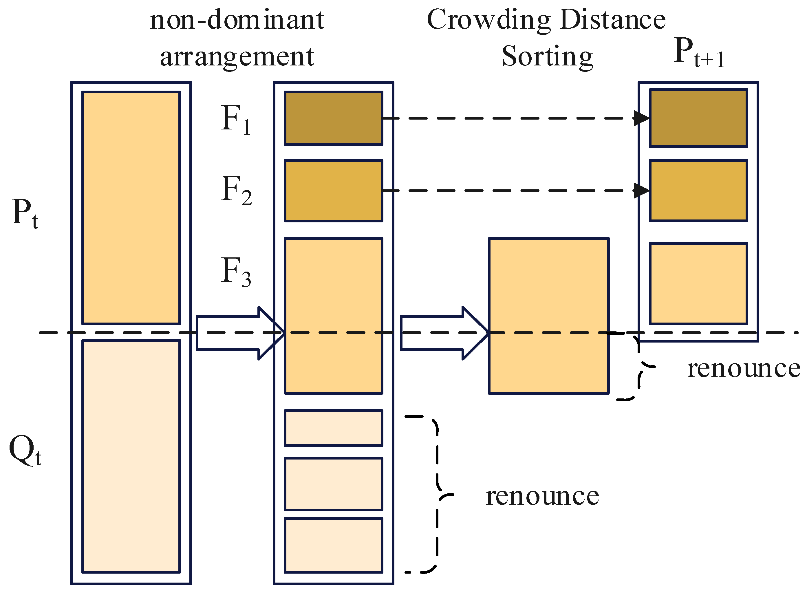
Let the parent population be Pt, with size M. Generate the offspring population Qt, also of size M, using the selection, crossover, and mutation operators of the genetic algorithm. Combine the parent and offspring populations to form a new population Rt, whose size becomes 2M.
- (2)
Perform non-dominated sorting on population Rt, producing non-dominated solution sets of different ranks F1, F2, F3,…
- (3)
Calculate the crowding distance values for all individuals in each Fi and sort them.
- (4)
Based on the non-dominated sorting rank and crowding distance values, select the better individuals to be passed on to the next generation Pt+1.
The elitist strategy adopted by NSGA-II can significantly improve the performance of the genetic algorithm. This strategy passes excellent individuals to the next generation through operator calculations, avoiding issues like local optima and unstable evolution processes. It leads to a more uniform distribution of the Pareto-optimal solution set for multi-objective optimization problems, correspondingly improving the quality of the optimal solutions and thus obtaining more representative non-dominated solutions. The schematic diagram of this algorithm is shown in
Figure 3.
3.2. TOPSIS Decision Method
The Technique for Order Preference by Similarity to Ideal Solution (TOPSIS) is an effective method commonly used in multi-criteria decision analysis. This method ranks alternative solutions based on their relative closeness to ideal solutions. The basic steps of this method are:
- (1)
For n evaluation alternatives, select p evaluation indicators for comprehensive evaluation (if there are negative or moderate indicators among the evaluation indicators, convert them into positive indicators), constructing the original data matrix as:
- (2)
Construct the normalized decision matrix. Use a normalization method to standardize the decision variables, expressed as:
- (3)
Determine the ideal solutions for the decision problem: the positive ideal solution (PIS) and the negative ideal solution (NIS). These are the solutions where each attribute indicator reaches its best and worst value among all alternatives, respectively.
- (4)
Calculate the Euclidean distance from each alternative to the PIS and NIS.
- (5)
Calculate the relative closeness of each evaluation alternative to the ideal solutions. Based on the relative closeness value, select the alternative that is closest to the PIS and farthest from the NIS.
Sort according to the relative closeness Ci. The larger Ci, the closer the i-th evaluation alternative is to the optimal level.
It is important to clarify the computational advantage provided by the deep learning-based aggregator model. In traditional bilevel optimization frameworks, the lower-level aggregator optimization problem must be solved repeatedly within each iteration of the upper-level DNO optimization, resulting in computationally expensive nested loops. For instance, if the upper-level NSGA-II algorithm requires 100 iterations with a population size of 100, and each individual evaluation necessitates solving the aggregator’s optimization problem, this would lead to 10,000 lower-level optimization calls.
In contrast, the proposed approach replaces the lower-level optimization with a pre-trained deep learning model. Once trained offline, the neural network can predict the aggregator’s clearing strategy through a simple forward propagation in milliseconds, given the price signals and forecast information. This eliminates the need for real-time optimization at the lower level. However, the upper-level DNO optimization still requires an iterative process (as described in
Section 3.3) to search for the optimal Pareto front across multiple objectives. The key difference is that each iteration now involves only a rapid neural network inference rather than solving a complex constrained optimization problem, thereby significantly reducing the overall computational time.
To summarize, the deep learning model eliminates the lower-level iterative optimization, but the upper-level NSGA-II algorithm still iterates to find optimal solutions. This represents a shift from a nested bilevel iterative structure to a single-level iterative structure with fast aggregator response prediction.
3.3. Multi-Objective Optimization Process
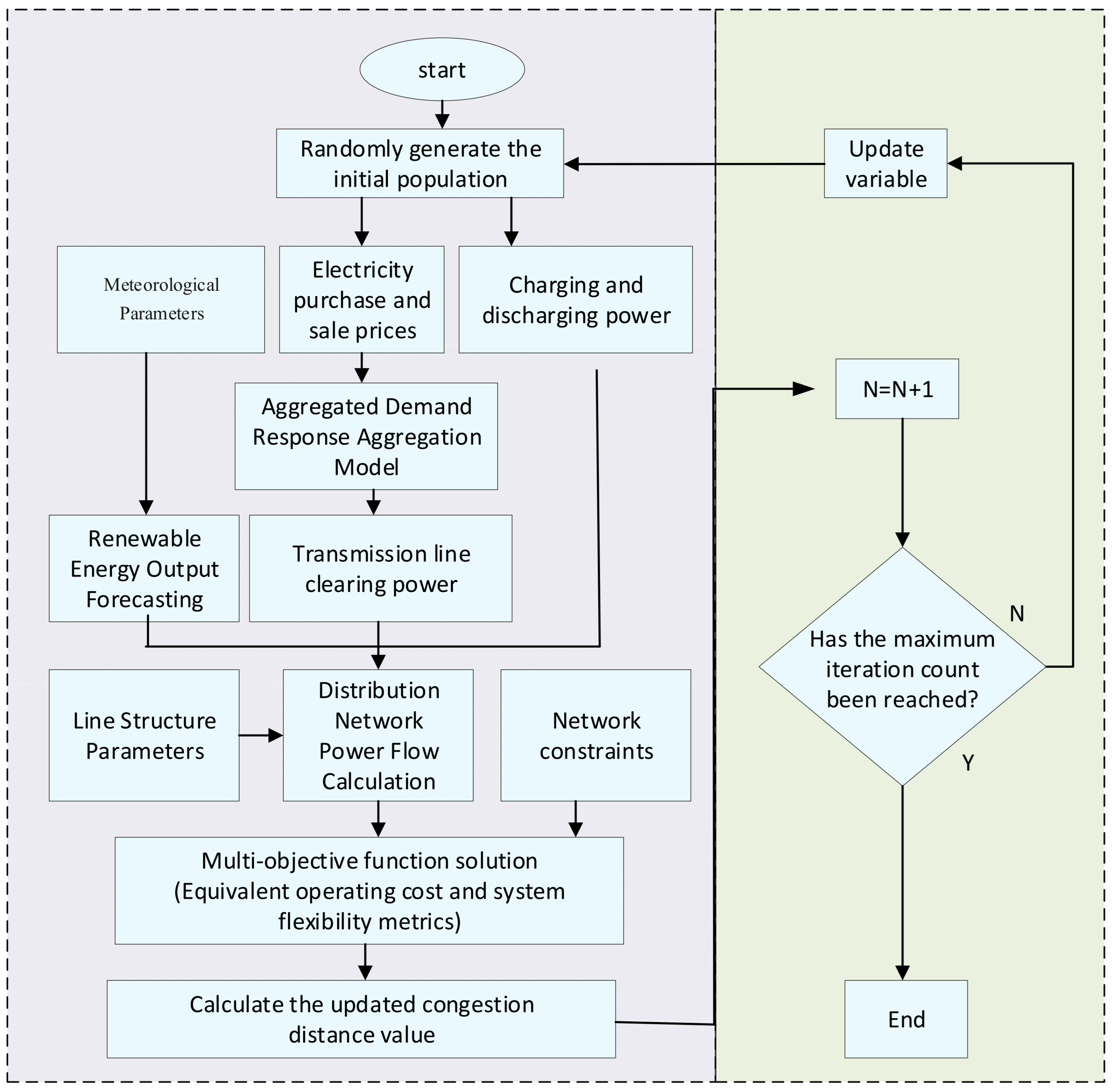
The specific flowchart of the algorithm proposed in this paper is shown in
Figure 4. The main steps of the NSGA-II-TOPSIS multi-objective optimization method adopted in this chapter are as follows:
Step 1: Initialize the genetic algorithm operator population, randomly generating the electricity purchase/sale prices from the DNO to aggregators, the output of DG, and the charging/discharging power of energy storage batteries.
Step 2: Based on the day-ahead electricity price information provided by the distribution network and external meteorological information, predict the electricity purchase/sale strategies of each aggregator through the deep learning network and generate clearing results.
Step 3: Input the clearing data of each aggregator, the output of DG, and the charging/discharging power data of energy storage batteries into the corresponding nodes of the distribution system. Combined with information from other nodes of the distribution network, calculate the multi-objective optimization function of the DNO through power flow calculation and node constraints. Record and update the crowding distance values in the NSGA-II algorithm, selecting the optimal individuals to pass to the next generation population.
Step 4: Determine whether the iteration count of the NSGA-II optimization has reached the maximum. If yes, terminate the optimization and output the optimal prices; otherwise, update the day-ahead prices, DG output, and energy storage battery charging/discharging power according to the DNO’s day-ahead price intervals.
Step 5: Return to Step 2 for iterative operation.
Step 6: Upon completion of iterations, use the TOPSIS rule to find the optimal price solution from the Pareto solution set, the optimal output distribution for DG, and the optimal day-ahead charging/discharging power schedule for energy storage batteries.
4. Case Studies
4.1. Simulation Scenario Design
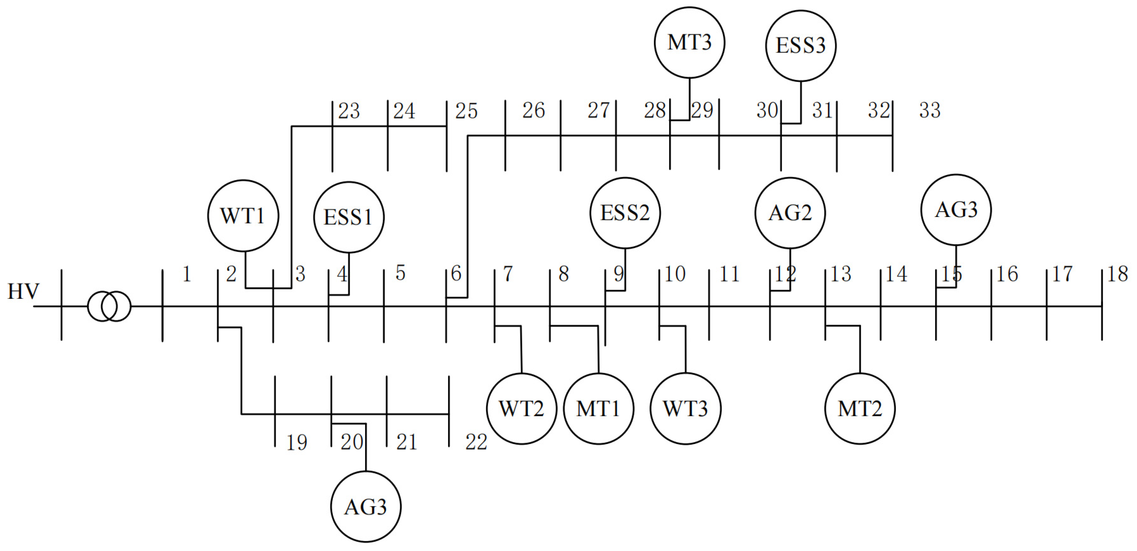
To verify the effectiveness of the proposed algorithm, simulation verification was conducted on a modified IEEE 33-node distribution network system. The structure of the distribution network is shown in
Figure 5. In the IEEE 33 system, the rated voltage at each node is 12.66 kV. The upper and lower limits of node voltage are set to 105% and 95% of the rated voltage, respectively. The distribution network is connected to the upstream grid via node 1. This section primarily studies the impact of integrating distributed renewable energy into the distribution network. By dispatching distributed generation and energy storage systems, adjusting clearing prices for aggregators to guide their rational electricity consumption, the goal is to enhance the economic efficiency and flexibility of distribution network operation.
Distributed wind power stations are connected to distribution network nodes 3, 7, and 10, with their predicted output assumed equal to actual output, and the electricity price is set at 0.02857 USD/kWh. Energy storage batteries are connected to nodes 4, 9, and 30, each with a rated capacity of 800 kWh, charging/discharging power of 400 kW, charge/discharge efficiency of 0.95, initial state of charge (SOC) of 20%. The minimum and maximum SOC for the batteries are set at 20% and 95%, respectively, with a maintenance cost of 0.01429 USD/kWh. Distributed generation using gas turbines is connected to nodes 8, 13, and 28, each with a rated power of 500 kW, ramp-up/down limits of 150 kW/h, and an electricity price of 0.05000 USD/kWh. Aggregators are connected to nodes 12, 15, and 20, with electricity prices following a time-of-use (TOU) tariff (peak, flat, valley) obtained through (game) the distribution network operator. The net load parameters for a typical day in the distribution network are shown in
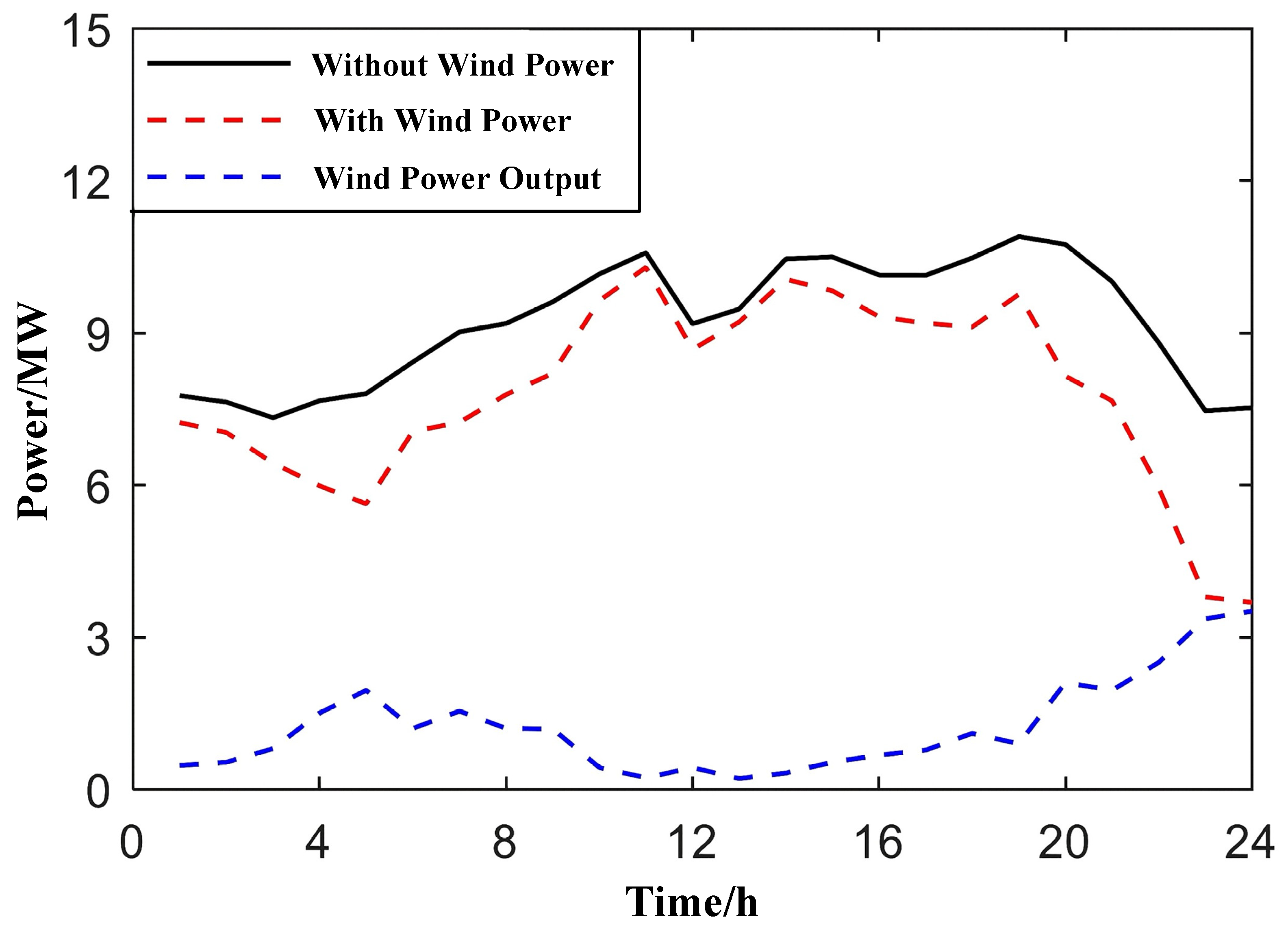
Table 1. The rated power of the wind power stations connected at the three nodes is 1.5 MW each. Under a typical day scenario, without considering aggregator participation or other dispatchable distributed resources in the optimization, the net load curves of the distribution network for two cases—without and with all wind farms connected—are shown in
Figure 6.
From the net load curve, it can be observed that with wind power integration, the peak points of the net load curve decrease slightly, while the valley points decrease significantly. The peak-to-valley load difference increases, potentially leading to insufficient downward adequacy of net load in the distribution system. Simultaneously, the fluctuation rate of the net load curve increases. For instance, during periods like 4:00–8:00 and 22:00–24:00, the corresponding flexibility of the distribution network decreases. Therefore, the randomness of distributed renewable energy can lead to situations where renewable output is high when system load demand is low, and vice versa. This inverse relationship can affect the penetration level of renewable energy and further cause a reduction in the flexibility of the distribution system. Consequently, to fully mitigate the problems brought by integrating renewable energy into the grid, it is essential to fully utilize the roles of distributed generation, energy storage systems, and aggregators within the system, formulate reasonable electricity price mechanisms, and optimally dispatch internal flexible response resources, thereby enhancing the economic security and flexibility of distribution network operation.
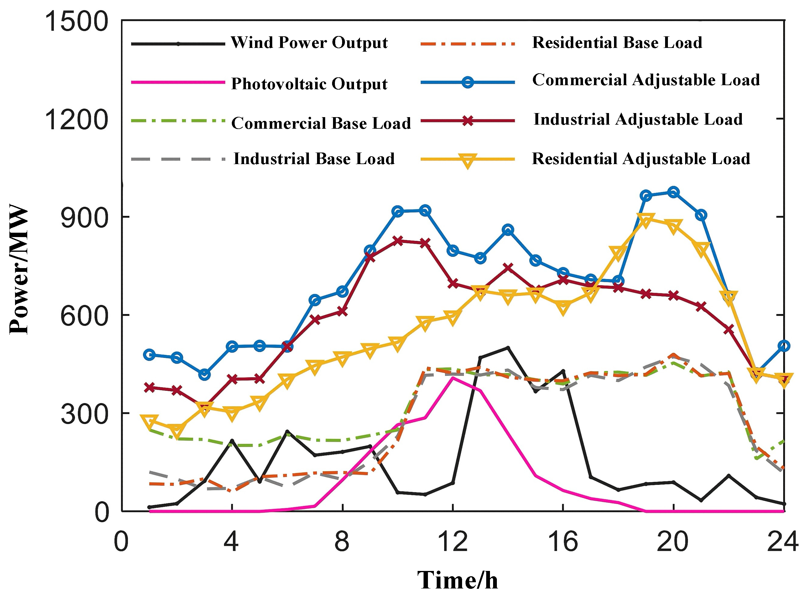
The primary resources managed within an aggregator include wind turbines, photovoltaic (PV) stations, dispatchable loads (e.g., air conditioning loads), and energy storage batteries. Aggregators are considered to participate in dispatch only with active power; their reactive power is randomly distributed between 0.85 and 0.99. Each aggregator internally has a 500 kW PV station, a wind turbine, and energy storage with a rated capacity of 500 kWh (Smin = 0.4, Smax = 0.95), charging/discharging power of 120 kW, and charge/discharge efficiencies of 0.9. To maintain battery lifespan, the number of charge/discharge cycles within one period is limited to 8. The flexible loads within the aggregator are primarily curtailable loads like air conditioning. Aggregator 1 represents commercial load; Aggregator 2, industrial load; Aggregator 3, residential load. The primary participation period for industrial curtailable loads is 9:00–18:00, while for residential and commercial loads, it is 11:00–22:00. The maximum and minimum continuous response duration per event is constrained to 2 h, with a daily limit of 5 dispatchable events. This section assumes the predicted output curves for wind and PV power are the same for all three aggregators. The specific load and renewable generation prediction curves are shown in
Figure 7.
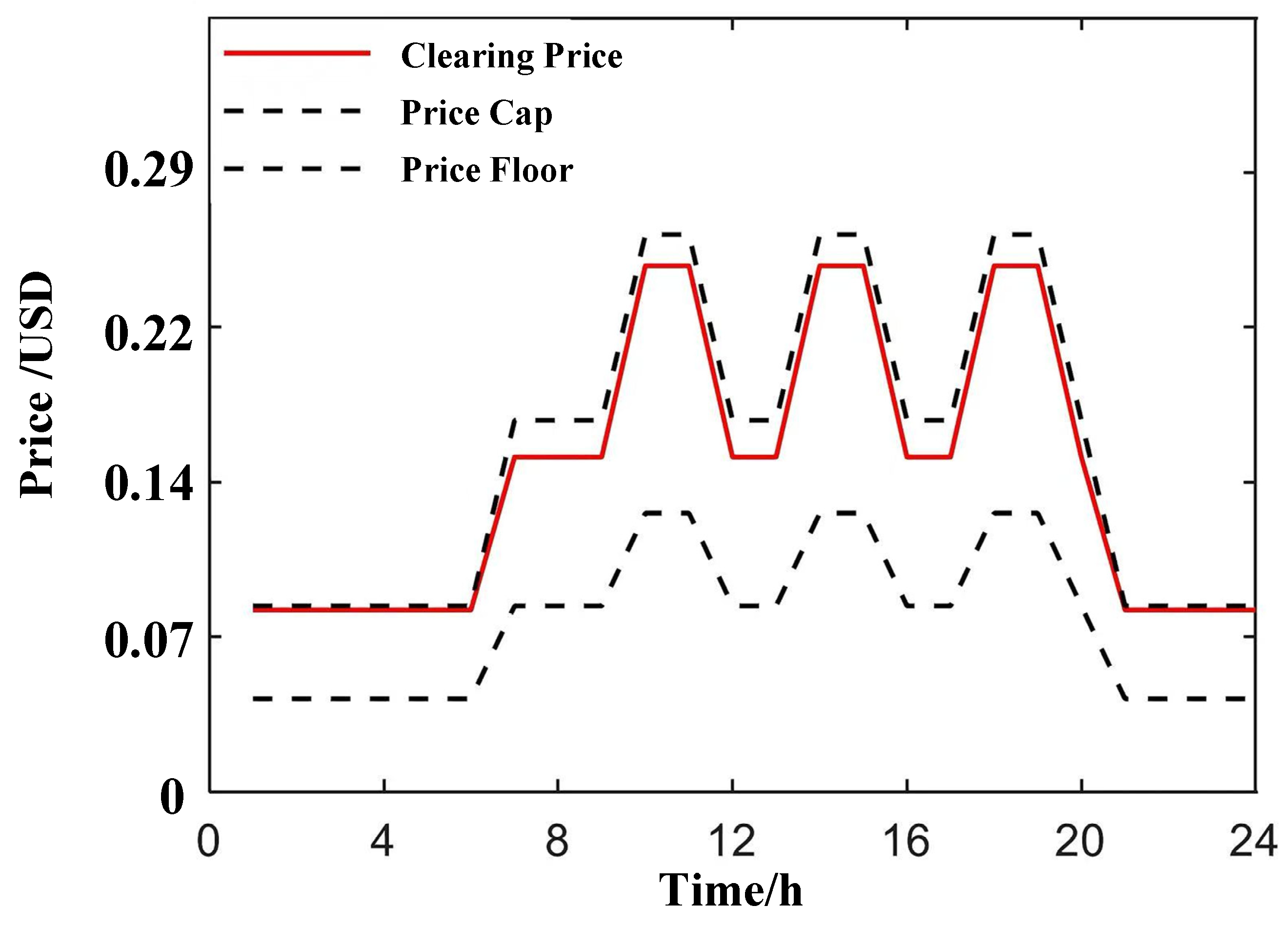
The distribution network employs a TOU pricing mechanism for electricity purchase and sale with aggregators. Since the DNO considers its own profit as a primary optimization objective when setting prices, there is a possibility of arbitrarily raising selling prices to obtain high profits. Therefore, corresponding constraints need to be considered when setting prices. A baseline price is set as the price upper limit, meaning the DNO’s pricing cannot exceed this baseline. The price lower limit is set at 50% of the baseline price. The baseline price periods are: peak hours (9:00~11:00, 13:00~15:00, 17:00~19:00) with selling price at 0.25714 USD/kWh and purchase price at 0.17857 USD/kWh; flat hours (6:00~9:00, 11:00~13:00, 15:00~17:00, 19:00~20:00) with selling price at 0.17143 USD/kWh and purchase price at 0.11429 USD/kWh; valley hours (0:00~6:00, 20:00~24:00) with selling price at 0.08571 USD/kWh and purchase price at 0.05714 USD/kWh. In this section, aggregators primarily act as net flexible resources participating in demand response; thus, the focus is on the DNO’s selling price to them.
4.2. Uncertainty Considerations and Sensitivity Analysis
While the base case study assumes perfect forecasts of renewable generation for clarity of analysis, we acknowledge that forecast errors are inevitable in practical operations. To address this concern, we provide the following discussion on how the proposed framework handles forecast deviations:
- (1)
Robustness of the Deep Learning Model: The training dataset includes diverse renewable generation profiles covering a wide range of weather conditions and seasonal variations. This diversity enables the trained model to generalize well to scenarios with moderate forecast errors. As long as the actual renewable output falls within the range covered by the training data (wind speeds 3–15 m/s, solar irradiance 0–1000 W/m2), the aggregator response prediction remains reasonably accurate.
- (2)
Implicit Uncertainty Handling: The multi-objective optimization framework inherently provides some robustness against uncertainties. By minimizing both operational cost and net load fluctuation rate, the NSGA-II algorithm tends to favor solutions with smoother power profiles and more conservative resource utilization, which naturally reduces vulnerability to forecast errors.
- (3)
Sensitivity Analysis: To quantitatively assess the impact of renewable forecast errors, we conducted a post-optimization sensitivity analysis. The optimal dispatch solution obtained under a perfect forecast was re-evaluated under scenarios where actual renewable generation deviates from the forecast by ±10%, ±20%, and ±30%. The results are summarized as follows:
“±10% deviation”: The actual operational cost increases by 2.3–3.8% compared to the optimal cost under perfect forecast. The net load fluctuation rate increases by 4.1–5.6%. The system remains feasible with no voltage or line capacity violations.
“±20% deviation”: The actual operational cost increases by 5.7–8.2%. The net load fluctuation rate increases by 9.3–12.7%. Minor voltage deviations (within ±3% of nominal) occur at peripheral nodes during peak hours, but no critical violations are observed.
“±30% deviation”: The actual operational cost increases by 10.1–14.6%. The net load fluctuation rate increases by 17.2–23.5%. Voltage violations (exceeding ±5% limit) occur at 2–3 nodes during extreme mismatches between forecast and actual output. In these cases, the energy storage system absorbs excess renewable generation or compensates for deficits, preventing cascading failures.
The sensitivity analysis demonstrates that the proposed framework maintains acceptable performance under moderate forecast errors (within ±20%), which is consistent with typical day-ahead forecasting accuracy reported in the literature (MAPE of 10–20% for wind power and 5–15% for photovoltaic power). For more severe deviations, additional real-time corrective measures (e.g., intraday re-dispatch or emergency demand response activation) would be required, which is beyond the scope of this day-ahead optimization framework.
It is also worth noting that integrating stochastic or robust optimization into the proposed framework represents a promising direction for future work. Scenario-based stochastic programming could explicitly model probabilistic renewable generation forecasts, while robust optimization could guarantee feasibility under worst-case deviations within bounded uncertainty sets. Such extensions would further enhance the framework’s practical applicability, and the authors plan to investigate these approaches in subsequent research.
4.3. Analysis of Aggregator Deep Learning Model Simulation Results
The demand response training models for the three aggregators in the distribution network were developed using the TensorFlow 2.0 framework in Python 3.7. During model construction, market electricity price, temperature, solar irradiance, wind speed, and constraint parameters for dispatchable loads and energy storage were selected as input parameters, with demand response as the output decision. Each model has the same structure, featuring a horizontal combination arrangement of two Long Short-Term Memory (LSTM) layers, two Convolutional Neural Network layers, and two Gated Recurrent Unit (GRU) layers. The two 1D convolutional layers (Conv1D) have 32 and 128 filters, respectively. The two LSTM layers have 32 and 128 neurons, respectively. The two GRU layers have 16 and 16 units, respectively. The activation function for all three neural network types is ReLU. After training with constructed samples, the mean absolute percentage error (MAPE) for the test set clearing decisions of the three aggregators was 1.89%, 2.35%, and 2.38%, respectively. Therefore, the deviations between the clearing decisions of the three aggregators and the actual values are small, justifying the application of the deep learning-based intelligent decision-making ensemble model to the game model between aggregators and the distribution network in the day-ahead electricity market trading.
The complete architecture of the proposed Inception-based deep learning model is detailed as follows:
“Input Layer”: The input layer accepts multi-dimensional time-series data with a shape of (batch_size, 24, 7), where 24 represents the 24 h time steps and 7 represents the feature dimensions, including hourly electricity price, wind speed forecast, solar irradiance forecast, temperature forecast, load baseline, energy storage SOC, and constraint parameters.
“Parallel Feature Extraction Branches”: The Inception structure consists of three parallel branches to capture multi-scale temporal patterns:
“CNN Branch”: Two one-dimensional convolutional layers (Conv1D) with 32 and 128 filters, respectively. The first layer uses a kernel size of 3 with stride 1, and the second layer uses a kernel size of 5 with stride 1. Both layers employ ReLU activation functions and are followed by batch normalization to accelerate convergence and improve generalization.
“LSTM Branch”: Two stacked LSTM layers with 32 and 128 hidden units, respectively. The LSTM branch is designed to capture long-term temporal dependencies in the input sequences. Dropout with a rate of 0.2 is applied between the two LSTM layers to prevent overfitting.
“GRU Branch”: Two stacked GRU layers with 16 and 16 hidden units, respectively. The GRU branch provides an alternative recurrent structure with fewer parameters, complementing the LSTM branch in modeling temporal dynamics.
“Feature Fusion Layer”: The outputs from all three parallel branches are concatenated along the feature dimension, resulting in a comprehensive feature representation that combines multi-scale spatial patterns (from CNN) and temporal dependencies (from LSTM and GRU).
“Fully Connected Layers”: Two dense layers with 256 and 128 neurons respectively, are applied after feature fusion. Both layers use ReLU activation and are followed by dropout (rate = 0.3) to enhance model robustness.
“Output Layer”: The final output layer consists of 72 neurons corresponding to the 24 h clearing strategy decisions (24 h power exchange + 24 h energy storage schedule + 24 h load adjustment). Linear activation is used for the output layer to allow continuous value predictions.
“Training Configuration”: The model was trained using the Adam optimizer with an initial learning rate of 0.001, which decays by a factor of 0.5 if validation loss does not improve for 10 consecutive epochs. The batch size was set to 64, and training was conducted for a maximum of 200 epochs with early stopping (patience = 20 epochs) based on validation loss. The loss function is mean squared error (MSE) between predicted and actual clearing strategies. Training was performed on a standard computing platform equipped with an NVIDIA GPU, and convergence was typically achieved within 80–120 epochs, requiring approximately 2–3 h of training time.
“Model Performance”: After training, the model achieved a mean absolute percentage error (MAPE) of 1.89%, 2.35%, and 2.38% on the test sets for the three aggregators, respectively, demonstrating high prediction accuracy. The inference time for a single prediction is approximately 15 milliseconds, which is several orders of magnitude faster than solving the original optimization problem (typically 5–10 s per instance).
4.4. Analysis of Distribution Network Optimal Operation Results
Based on the distribution network optimization algorithm proposed in
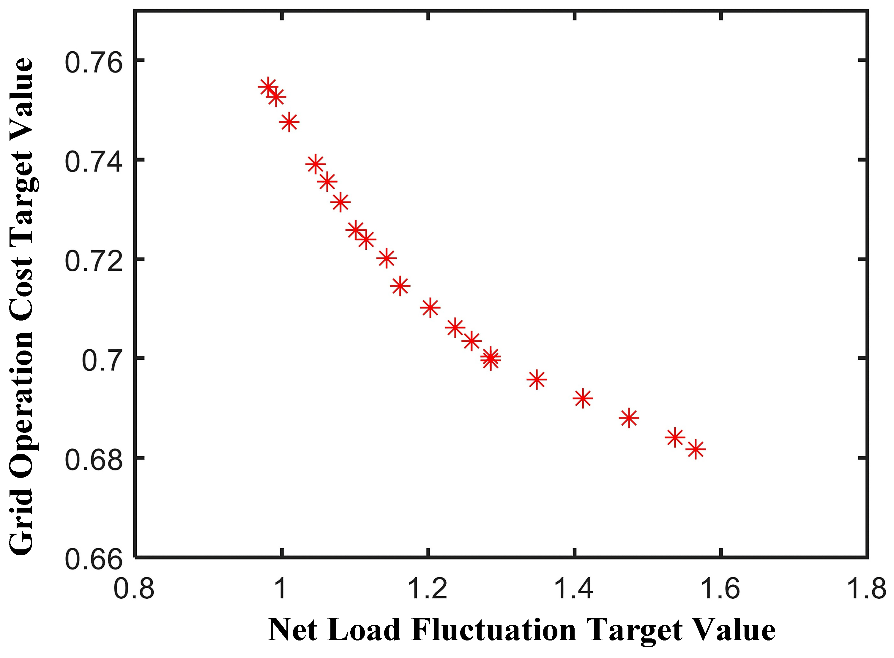
Section 4 of this chapter, the multi-objective optimization operation model between the DNO and the aggregators is solved. This chapter temporarily does not consider cooperation among multiple aggregators, meaning each aggregator interacts independently with the DNO, and the DNO applies the same clearing price to each aggregator. The proposed model is solved using the NSGA-II algorithm. The resulting Pareto-optimal solution set curve is shown in
Figure 8, containing 20 non-dominated solutions with good distribution characteristics. The TOPSIS rule is used to find the optimal ideal solution from the Pareto front. The corresponding equivalent value for the operational cost under the optimal dispatch scheme is 0.731, while the net load fluctuation rate is 1.081.
According to the optimal operational objective values found by the TOPSIS rule, the final transaction electricity prices between aggregators and the DNO are shown in
Figure 9. The data shows that under the optimal solution, the DNO primarily sells electricity to aggregators. The selling prices for each period are as follows: peak hours: 0.24257 USD/kWh, flat hours: 0.15443 USD/kWh, valley hours: 0.08386 USD/kWh.
To further analyze the characteristics exhibited by different optimization objective values,
Table 2 presents the two boundary values from the Pareto solution, i.e., the TOU price solutions corresponding to the minimum equivalent operational cost and the minimum tie-line power fluctuation, and compares them with the optimal solution selected using the TOPSIS rule. From the table, it is not difficult to see that when the equivalent operational cost is minimized, the DNO’s selling price is correspondingly the highest. At this point, the DNO increases its profit by raising the price, i.e., reducing the equivalent cost. However, the corresponding tie-line power fluctuation is the largest, indicating insufficient motivation of aggregators to meet the distribution network’s flexibility requirements. In contrast, when the DNO lowers prices, increases the price differential between peak, flat, and valley periods, and provides sufficient incentives, aggregators demonstrate greater initiative. This effectively reduces peak loads, increases valley loads, and mitigates the fluctuation rate of the net load curve. Therefore, for the DNO, a balance between the two objectives can be considered to select an optimal strategy, achieving reduced equivalent operational costs while ensuring power fluctuation remains within a reasonable range, meeting both economic and flexibility needs of the grid.
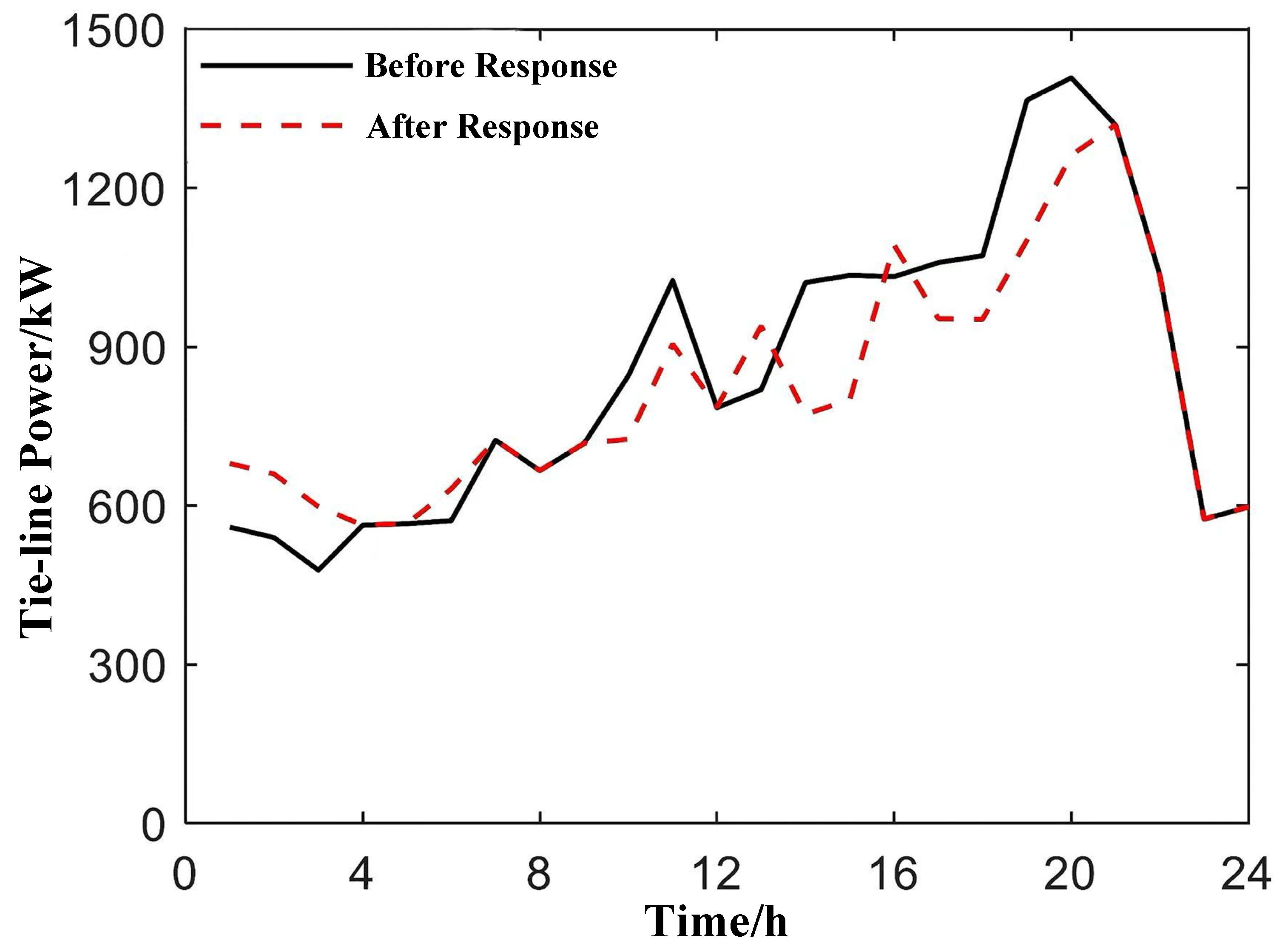
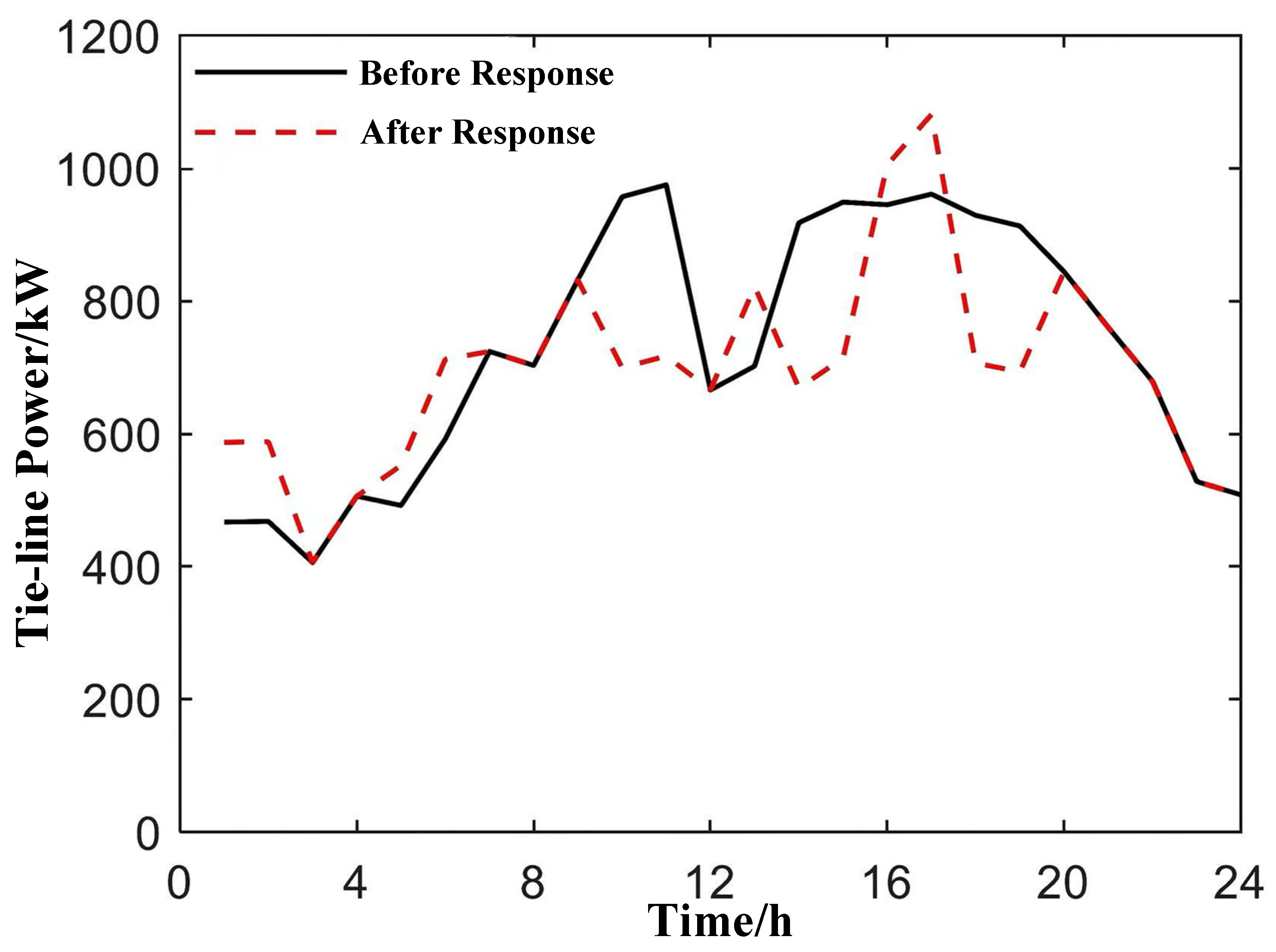
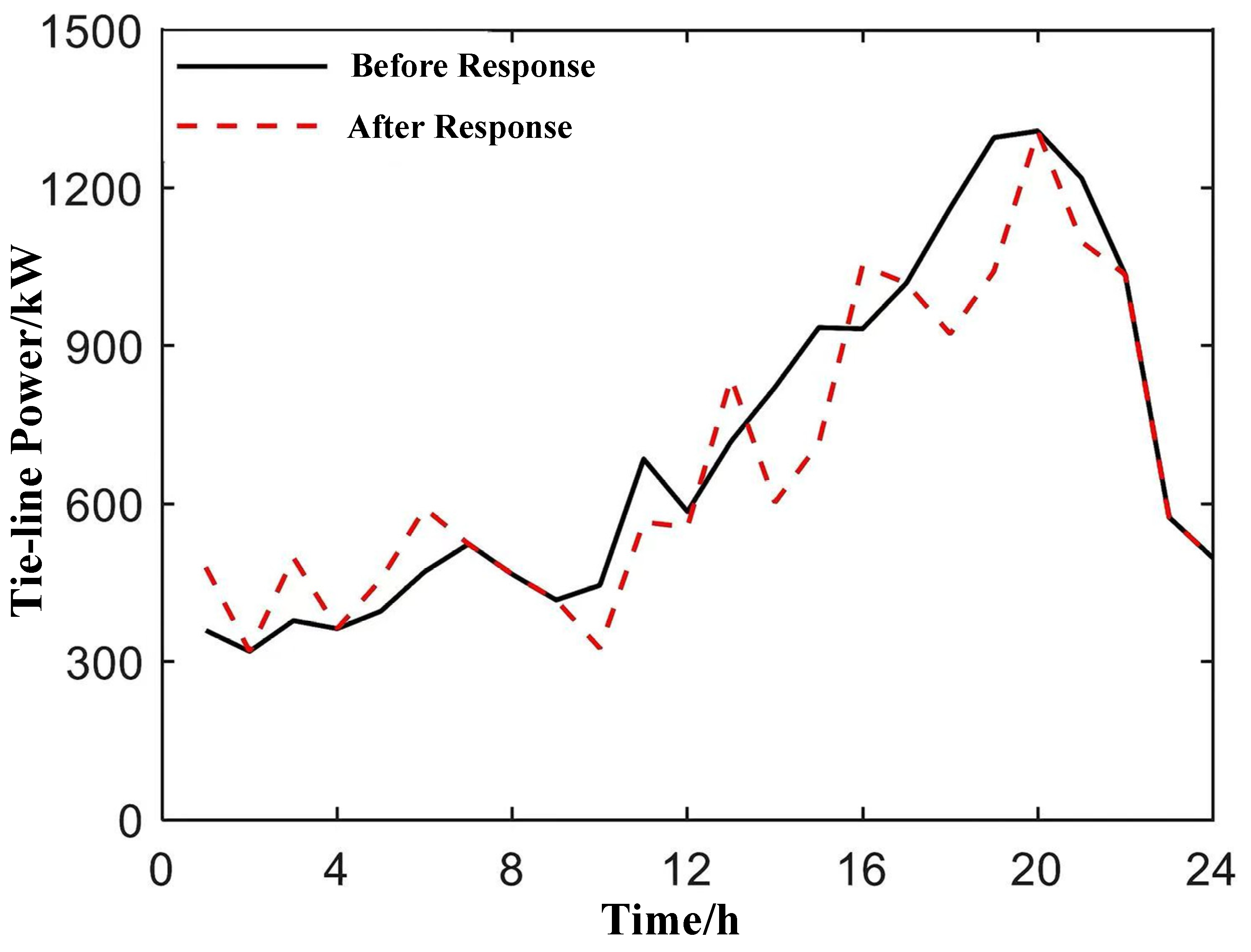
Under the optimal solution of the objective functions, analyzing the response decisions of each aggregator reveals the comparison results of their demand response strategies before and after participating in the day-ahead electricity market trading, as shown in
Figure 10,
Figure 11 and
Figure 12.
The ‘before response’ curve represents the initial load demand of the aggregator when not considering cost minimization as an objective, i.e., when internal flexible loads do not participate in demand response. The ‘after response’ curve represents its power purchase strategy after participating in demand response under the final agreed electricity price trading strategy. Combining this with the previously obtained price results, it can be observed that the main purpose of adjustment for aggregators is their own economic cost regulation needs. Therefore, based on the agreed price transaction, they shift and curtail consumption during peak price hours. During flat or valley price hours, energy storage plays a major regulatory role, supporting the grid’s peak shaving and valley filling.
In the current simulation setup, all three aggregators receive the same time-of-use pricing signals from the DNO. This uniform pricing strategy is adopted for practical reasons: it reflects widely used retail tariff structures and avoids the complexity of locational pricing (which would require network topology disclosure and increase coordination difficulty). Although the price signals are identical, the three aggregators exhibit distinct response profiles (
Figure 10,
Figure 11 and
Figure 12) due to differences in their resource compositions (commercial, industrial, residential), and their diverse responses collectively improve the network’s operational flexibility. Investigating differentiated pricing strategies is left for future research.
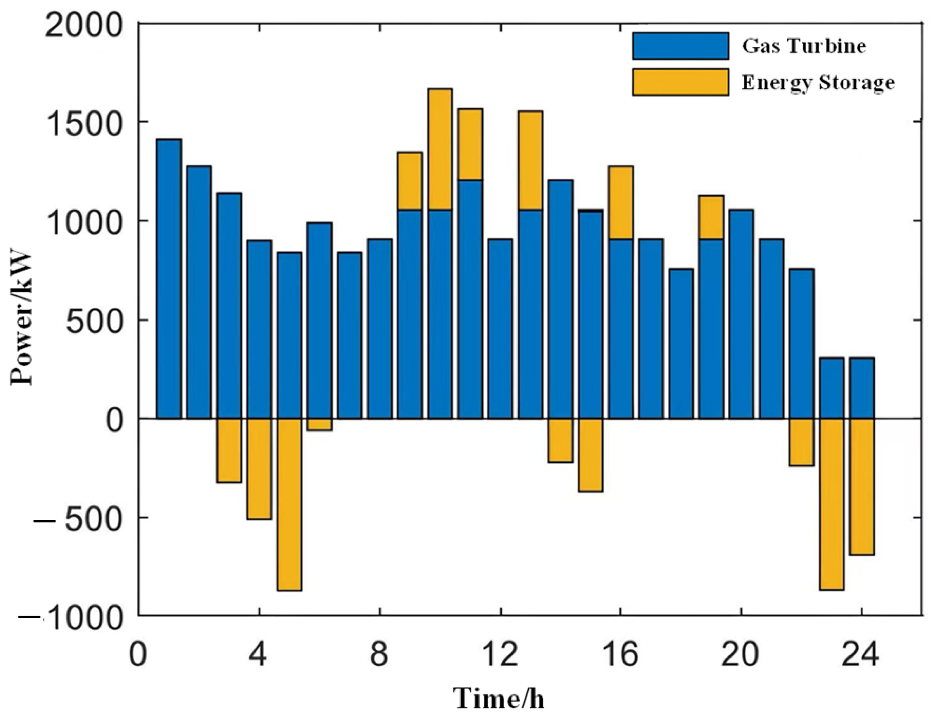
Figure 13 shows the output distribution of gas turbines and the charging/discharging schedules of energy storage batteries after distribution network dispatch. Positive storage values represent discharging; negative values represent charging. During periods of low wind power output and high electricity load within the distribution network, such as 9:00–13:00 and 16:00–19:00, both gas turbines and energy storage output significant power to meet the line net load demand. Simultaneously, during moments of high fluctuation within these periods, such as 12:00–13:00 and 17:00–19:00, gas turbines and energy storage adjust appropriately by reducing output power to meet the need for load fluctuation smoothing. Conversely, during periods of low load demand and high wind power output, such as 3:00–6:00 and 22:00–24:00, gas turbines correspondingly reduce output, and energy storage is in a charging state. By coordinating the control of gas turbines and energy storage batteries based on its real-time operational needs, the distribution network achieves the effects of peak shaving, valley filling, and load fluctuation smoothing.
4.5. Analysis of Distribution Network Operational Flexibility Enhancement
Taking operational flexibility indicators as one of its optimization objectives, the distribution network aims to meet the corresponding characteristics of flexible system operation by reasonably guiding user-side aggregators through pricing and effectively controlling distributed generation and energy storage batteries. To verify the effectiveness of the proposed method in enhancing grid operational flexibility, three scenarios are constructed for comparative analysis.
- (1)
Scenario 1: Only gas turbines within the distribution network participate as distributed generation in the regulation operation of the distribution network;
- (2)
Scenario 2: Both gas turbines and energy storage batteries within the distribution network are considered to participate in the dispatch;
- (3)
Scenario 3: The proposed method in this chapter, where gas turbines, energy storage batteries, and aggregators collectively act as flexible dispatchable resources participating in the day-ahead operation regulation of the distribution network.
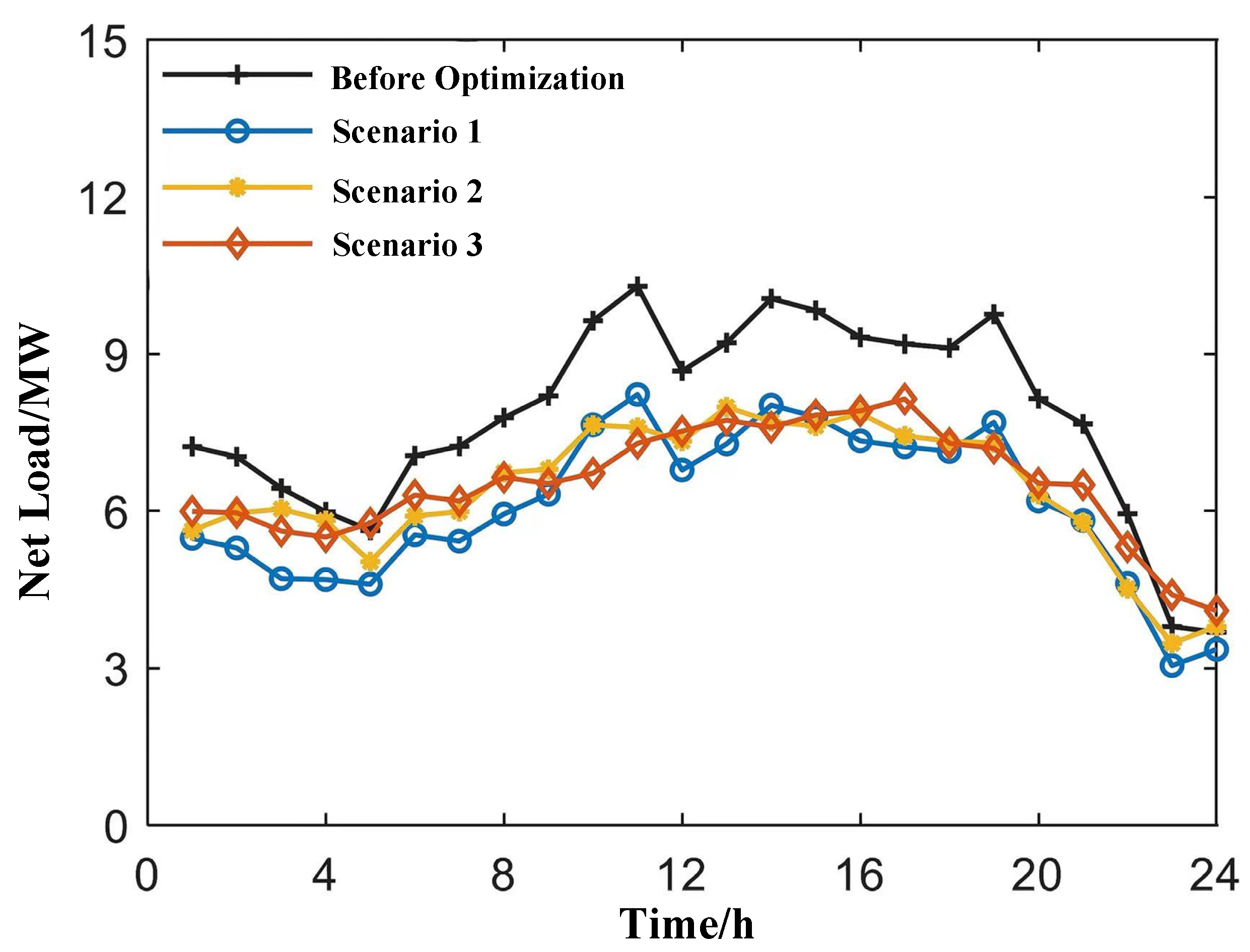
Based on the three different dispatch methods,
Figure 14 presents a comparison of the distribution network’s net load curves under different scenarios before and after optimization. The figure shows that all three scenarios can effectively reduce the peak of the day-ahead operation. In Scenario 1, since only gas turbines are used for system regulation, they still output during valley periods due to economic needs, further lowering the system’s minimum load. The flexible resources in Scenarios 2 and 3 are more abundant compared to Scenario 1. In Scenario 2, energy storage batteries can reduce the system’s peak-to-valley difference through charging and discharging processes. In Scenario 3, internal flexible resources of aggregators also actively participate in the response. The resulting net load curve of the distribution network becomes smoother compared to the other two scenarios. Specifically, the load magnitude during the valley period (22:00–24:00) in this scenario is significantly increased compared to others, while the load magnitude during peak periods (10:00–16:00 and 19:00–21:00) is effectively reduced. Overall, the peak-to-valley load difference decreases, and the net load fluctuation rate is smoother than in the other two scenarios.
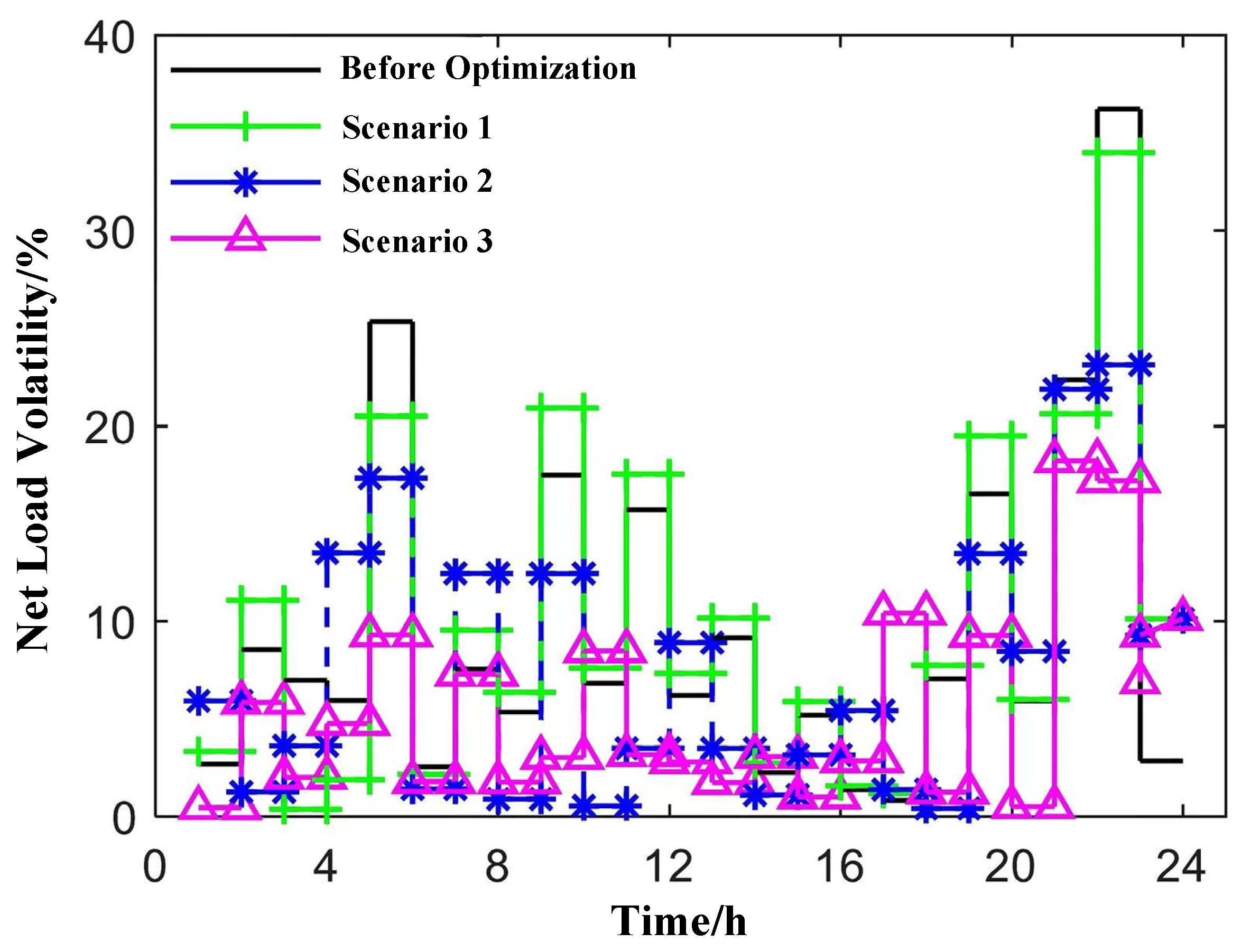
To further verify that regulating various types of internal flexible resources can meet operational flexibility requirements under increasing renewable energy penetration,
Figure 15 shows the distribution of the distribution network’s net load fluctuation rate under different operating scenarios. It can be observed that when no flexible resources participate in system response, significant load fluctuation rates occur around periods like 5:00–6:00, 11:00–12:00, and 20:00–22:00, with a maximum exceeding 30%. At this point, the distribution network’s flexibility requirements are inevitably affected. When this exceeds the maximum allowable fluctuation range of the distribution network itself, situations like wind curtailment or load shedding might occur to maintain system stability. In Scenario 1, where only gas turbines act as flexible resources for system regulation, the net load fluctuation rate of the distribution network is not significantly alleviated; in fact, it increases further at certain times, such as during 9:00–10:00, 11:00–12:00, and 19:00–20:00. Since gas turbines can only provide positive power for system regulation and cannot meet the need for negative power regulation required by the system (e.g., during high renewable output, low load periods), the corresponding load fluctuation rate instead increases. Both Scenarios 2 and 3 possess flexibility resources capable of bidirectional regulation, such as energy storage and aggregators. In these two scenarios, the net load fluctuation rate is effectively reduced. Especially in Scenario 3, the combined regulation of aggregators and energy storage batteries yields more prominent results, demonstrating the optimal net load fluctuation rate. Overall, by regulating multiple flexible resources and incentivizing aggregators to participate in distribution network operation management through a reasonable electricity price trading process, the net load fluctuation rate of the distribution network is significantly improved, with the indicator showing a notable decrease at most times.
The flexible adequacy of the distribution network’s net load reflects the operational characteristics of line power and is another important indicator of distribution network operational flexibility. The upward and downward flexible adequacy are calculated according to the definitions in
Section 2.2.1. Based on these formulas,
Table 3 presents the comparison results of the net load upward margin and downward margin values under different operating scenarios during two typical periods: peak hours and valley hours. In the table, the maximum allowable value for net load during peak hours is set to 10 MW, and the minimum allowable value during valley hours is set to 4 MW.
The table shows that the upward and downward adequacy of the net load changes considerably before and after the participation of flexible resources in regulation. Before the response, both upward and downward adequacy levels are significantly lower. At 13:00–15:00, the upward adequacy values are 7.86%, −0.58%, and 1.69%, respectively. At 23:00–24:00, the downward adequacy values are −5.16% and −7.87%, respectively, indicating insufficient flexibility in both upward and downward directions at that time. Scenario 1 shows a relatively obvious improvement in upward adequacy during peak hours (13:00–15:00), increasing to 19.78% at 14:00. Scenarios 2 and 3 also demonstrate good capability in improving upward adequacy. After regulation, the distribution network exhibits sufficient upward flexibility margin. However, Scenarios 1 and 2 fail to fully improve the problem of insufficient downward system flexibility. Particularly in Scenario 1, since its flexible resources can only provide positive power, during periods of high renewable output and low system load demand (valley periods), the corresponding flexible resource (gas turbine) cannot provide the negative power demand needed by the system in the valley zone. Consequently, the system’s downward flexibility adequacy level instead decreases. Scenario 2 also has limited types of flexible resources. Energy storage batteries, constrained by their charging power limits, have limited response capability for improving system flexibility needs, so their improvement effect on the system flexibility level is not optimal. Scenario 3, in contrast, demonstrates excellent improvement in system net load adequacy levels. Through the combined regulation of energy storage batteries and aggregators, the system’s downward adequacy level during corresponding valley periods increases to 10% and 2.4%, respectively, improving the downward adequacy of system net load during valley periods and enhancing the system’s operational flexibility at those times.
Through the above analysis, the DNO dynamically regulates internal flexible resources and guides aggregators to actively participate in demand response through a pricing mechanism, changing the generation/consumption behavior of multiple types of demand-side resources. This meets the economic and flexibility operation requirements of the distribution network under increasing penetration of distributed renewable energy. When many aggregators participate in the grid’s market operation, using an intelligent decision-making module can enhance their demand response speed, reduce cumbersome iterative time with upper-layer grid optimization, and greatly improve model solving efficiency. After the DNO provides reasonable market prices, the adequacy level of system load is improved, the line net load fluctuation rate is effectively mitigated, and the corresponding operational flexibility of the distribution network is significantly enhanced, playing a positive role in further increasing the penetration rate of distributed renewable energy in the future.
4.6. Computational Efficiency Analysis
A key claimed advantage of the proposed framework is the significant improvement in computational efficiency compared to conventional bilevel iterative optimization. To substantiate this claim quantitatively, we compare the computational time of the proposed method against a baseline approach where the aggregator’s optimization problem is solved explicitly in each iteration.
Baseline Method: In the conventional bilevel approach, the lower-level aggregator optimization is formulated as a mixed-integer linear programming (MILP) problem and solved using CPLEX at each function evaluation within the NSGA-II algorithm. For a population size of 100 and 150 generations, this requires 100 × 150 = 15,000 MILP solver calls.
Proposed Method: The deep learning surrogate model replaces the MILP solver with a neural network forward pass. Each inference takes approximately 15 milliseconds compared to 5–8 s for the MILP solver. The computational time comparison is summarized in
Table 4 below.
The results clearly demonstrate that the proposed deep learning-based framework reduces the total optimization time by approximately 99.5%, from over 20 h to less than 10 min. This dramatic improvement in computational efficiency makes the proposed framework practically viable for day-ahead operational planning, where decisions typically need to be made within 1–2 h.
In addition to computational efficiency, the solution quality of the proposed DL surrogate model is validated by the low MAPE values (1.89–2.38%) reported in
Section 4.3, indicating that the aggregator responses closely approximate those obtained from explicit optimization-based baseline methods. Thus, the proposed method preserves accuracy while achieving a substantial reduction in computation time.
Regarding scalability, the computational burden grows linearly with the number of aggregators, as the DL model inference for each aggregator can be parallelized. The NSGA-II optimization for the distribution network itself scales moderately with network size (e.g., number of buses), which is typical for heuristic algorithms, but the elimination of lower-level iterations remains beneficial regardless of network scale.
It should be noted that the offline training of the deep learning model requires approximately 2–3 h. However, this training is performed only once (or periodically updated when significant changes in system operation occur), and the trained model can be reused for daily optimization without additional training costs. Therefore, the total computational investment of the proposed approach is significantly lower than that of the conventional method when evaluated over a typical operational period of one month or longer.




 and
and