Networked Multi-Agent Deep Reinforcement Learning Framework for the Provision of Ancillary Services in Hybrid Power Plants

Abstract

Inverter-based resources (IBRs) are becoming more prominent due to the increasing penetration of renewable energy sources that reduce power system inertia, compromising power system stability and grid support services. At present, optimal coordination among generation technologies remains a significant challenge for frequency control services. This paper presents a novel networked multi-agent deep reinforcement learning (N—MADRL) scheme for optimal dispatch and frequency control services. First, we develop a model-free environment consisting of a photovoltaic (PV) plant, a wind plant (WP), and an energy storage system (ESS) plant. The proposed framework uses a combination of multi-agent actor-critic (MAAC) and soft actor-critic (SAC) schemes for optimal dispatch of active power, mitigating frequency deviations, aiding reserve capacity management, and improving energy balancing. Second, frequency stability and optimal dispatch are formulated in the N—MADRL framework using the physical constraints under a dynamic simulation environment. Third, a decentralised coordinated control scheme is implemented in the HPP environment using communication-resilient scenarios to address system vulnerabilities. Finally, the practicality of the N—MADRL approach is demonstrated in a Grid2Op dynamic simulation environment for optimal dispatch, energy reserve management, and frequency control. Results demonstrated on the IEEE 14 bus network show that compared to PPO and DDPG, N—MADRL achieves 42.10% and 61.40% higher efficiency for optimal dispatch, along with improvements of 68.30% and 74.48% in mitigating frequency deviations, respectively. The proposed approach outperforms existing methods under partially, fully, and randomly connected scenarios by effectively handling uncertainties, system intermittency, and communication resiliency.

1. Introduction

1.1. Background

The potential of ancillary services from inverter-based resources (IBRs) is evolving with the ongoing penetration of renewable energy sources. To effectively deliver frequency and non-frequency ancillary services, it is essential to develop advanced control techniques for non-synchronous generation [1]. A hybrid power plant (HPP) combines independent electricity generation and storage technologies connected at a single point to provide coordinated electrical power services. This integration optimises land use and increases profitability by enabling participation in various energy markets, including capacity, time-varying pricing, and ancillary services. However, due to grid code requirements, the provision of grid support and ancillary services from HPPs is still in the early stages of development [2]. Frequency-control ancillary services from HPPs are challenging due to the complexity and coordination of heterogeneous technologies. Several studies have explored conventional approaches that involve plant-level control by introducing time-varying set points [3,4], but have encountered challenges with communication delays, slower response, and optimal control. The grid-forming control schemes in IBR-enabled HPPs were investigated in [5] to provide coordinated droop control and inertial support for frequency regulation and mitigation of frequency deviations. In [6], an HPP-enabled environment was considered to investigate the system performance in relation to frequency deviation under highly intermittent situations. In this case, the HPP model was optimised by minimising the frequency overshoot and improving the frequency stability.

For real-time coordination in plant controllers, estimating frequency response by dispatching active power is discussed in [7]. However, this approach does not apply to HPP controllers due to the complexity of coordination control. Different levels of control that need to be coordinated include asset-level control, plant-level control, HPP-level control, and HPP energy management system (EMS) control, as shown in Figure 1 [8]. Thus, it becomes challenging for the HPP EMS control level to acquire time-sensitive frequency control ancillary services such as fast frequency response (FFR) and black start (BS) due to the inverter’s response on different control levels. IBR-enabled systems generate large volumes of data through metering and control systems, offering valuable opportunities for data-driven analysis. These insights can be used to develop practical solutions for frequency control, particularly through cooperative control schemes. System responses are monitored and optimised in these approaches to meet various control objectives [9]. These systems are optimised through tailored training protocols based on Markov chain principles, data-driven strategies, and multi-agent control schemes. Multi-agent reinforcement learning (MARL) schemes are employed for frequency stability using partial communication to enable synergy among controllers and promote cooperative behaviour across the network. Various studies have explored MARL for decentralised generation control and joint optimisation [10]. For example, Markov game theory and graph-theoretic approaches have been applied to frequency control services, where distributed control nodes work together to achieve global control objectives. However, these methods are often computationally inefficient for real-time coordination, and require precise tuning of parameters for accurate modelling and optimal results [11].

Reinforcement learning (RL) approaches are better suited for low-dimensional action domains, which limits their effectiveness in complex and data-intensive IBR-enabled environments. Deep reinforcement learning (DRL) addresses high-dimensional state-action processes, utilising deep neural networks (DNN) for processing high-dimensional data and RL for decision-making. In one study [12], DRL was applied to complex distribution networks to improve voltage stability and frequency control. Another study [13] used DRL with the deep deterministic policy gradient (DDPG) algorithm to optimise voltage fluctuations in PV networks with high solar penetration. Based on policy networks, DRL algorithms have been used to solve frequency control optimisation problems across low- and high-dimensional state-action spaces. For example, in [14], a multi-agent DRL (MADRL) framework was implemented for the bidding process in PV plants, aiming to maximise power utilisation and cost optimisation. Similarly, MADRL was proposed in [15] for optimal demand response (DR) in electric vehicle (EV) charging infrastructure to optimise performance. A comprehensive review of MADRL in [16] highlighted various DRL algorithms for high-dimensional data and assessed their robustness in addressing voltage and frequency stability issues. In [17], MADRL was proposed for real-time voltage stability control to enhance both the learning efficiency and robustness of DRL performance.

Multi-agent deep deterministic policy gradient (MADDPG) and deep-Q-network (DQN) schemes were proposed in [18] for time-sensitive applications to optimise the operation and performance of virtual power plants (VPP). MADDPG employs a decentralised actor-critic architecture in a multi-agent control environment. This setup enables global information access and centralised training, while agents make autonomous decisions based on local observations and execute them in a decentralised manner. For load frequency control (LFC) in multi-area power systems, MADRL has been applied to regulate global functions using local control signals to manage frequency fluctuations [19]. In [20], the authors discussed the possibility of real-time multi-agent coordination, however, optimal selection of hyperparameters poses challenges during fine-tuning and implementation. The MADRL approach proposed in [21] focused on optimising multi-carrier energy grids by utilising stacked denoising autoencoders to dispatch energy nodes hourly. Similarly, an MARL model was introduced in [22] to address optimal load scheduling, energy management, and dispatch challenges in complex energy systems. Both approaches aim to enhance the coordination and efficiency of energy distribution while optimising performance across varying energy nodes and loads [23]. In [24], multi-microgrid scheduling schemes were implemented using soft actor-critic (SAC) and multi-agent control techniques. Meanwhile, an RL-based approach was adopted in [25], utilising a Markov decision process (MDP) in the MADRL framework for timescale bidding in IBR-enabled PV plants. This method coordinates multiple agents by considering stored energy, solar generation, bidding decisions, and other generation sources, with historical data used to initiate real-time coordination and bidding processes in the environment. This approach has demonstrated high profitability and effective management of energy imbalances across multiple timescales [26]. However, it does not address optimisation improvement for numerous IBR-enabled technologies, such as wind and ESS.

Table 1. MADRL schemes for energy management applications.

Refs.	Energy Source	Coordinations	Algorithms	Scalability	Performance
[27]	BESS, DG	Decentralized	Q-learning	Low	Improves power dispatch
[28]	PV, ESS, WP	Centralized	MPC	Low	Energy scheduling
[29]	VPP	Distributed	Q-learning	Moderate	Energy cost optimization
[30]	Microgrid	Centralized	SAC, DDQN	Moderate	Enhances thermal management
[31]	PV, ESS	Distributed	MOPS	Low	Improves cost optimization
[32,33]	PV, WP, EV	Distributed	Dec-POMDP	Moderate	Marginal cost optimization
[34,35]	Smart grid	Centralized	Dec-POMDP	Moderate	Reduces frequency deviation
[36,37,38]	PV, WP, ESS	Decentralized	D3Q, MADDPG	Moderate	Fast convergence
[39,40,41]	WP, ESS, PV	Networked	SAC, DDQN	Moderate	Optimizes energy cost
[42,43,44]	WP, PV	Networked	DDPG, MAAC	Moderate	Energy scheduling
This paper	PV, WP, ESS	Networked	SAC, MAAC	High	Optimal dispatch and Reserve

summarises state-of-the-art MADRL schemes for power systems applications involving multiple energy sources, coordination schemes, various algorithms, network scalability, and control performance.

The techniques mentioned in Table 1 are focused on DNN architectures, which are mostly implemented for model-free and high-dimensional complex networks. However, DNN-based approaches often operate as black boxes during the training and execution phases when processing high-dimensional state-action data. This lack of transparency can sometimes result in significant failures, particularly when the model struggles to converge to optimal state and control functions [45]. In addition, several studies have suggested graph-theoretic approaches with MADRL-based models for maintaining voltage stability in complex distribution network systems. This approach uses transformers and graph neural networks (GNN) instead of actor-critic networks for centralised training and decentralised execution [46]. However, while this approach has been applied to optimise physical parameters such as voltage control and stability, it does not fully address the heterogeneity of agents or the nonlinear behaviour of IBR-enabled power networks. Additionally, power resource scheduling is critical for providing ancillary services, but it introduces further challenges when dealing with intermittent energy sources.

This paper presents a networked MADRL (N—MADRL) approach to address these challenges for frequency control services in HPP environments. The N—MADRL approach utilises physical control parameters to develop a model-free framework. This framework is independent of specific controller input data and is highly scalable, fully adaptive, and decentralised for coordinating PV, WP, and ESS plants. In addition, it offers real-time coordination, control synergy, and computational efficiency using stable baseline DRL algorithms. In light of the complexity and nonlinearity of the HPP environment, the N—MADRL model overcomes three key challenges: 1 developing a model-free environment to coordinate numerous energy assets in the HPP network; 2 reducing the intermittency of HPP assets in optimal dispatch, reserve management, and frequency control services; and 3 addressing system vulnerabilities and dynamic performance with a networked communication structure. The proposed N—MADRL scheme ensures fast responses and compliance with grid code requirements for the HPP network. In addition, it effectively manages decentralised coordination across different levels of the HPP system, ensuring the timely provision of optimal dispatch and frequency control services.

1.2. Contribution and Outline

Despite the advancements in coordination control and optimal dispatch of energy assets for harnessing frequency control services in HPP networks, the existing literature on MADRL model-free frameworks for various energy management applications is still in the early exploration stage. Several challenges must be addressed for a fully coordinated HPP environment to provide frequency control ancillary services. First, the conceptual framework of MADRL, discussed in [47,48], is focused on the small-scale aggregation of distributed energy resources (DER), and does not fully exploit the utility-scale HPP environment through networked coordination control. Second, existing models rely on physical constraints and control parameters for the delivery of optimal dispatch [49], reserve management [50], and voltage control [51] based on cost optimisation, lacking focus on dynamic and performance-based control functions for utility-scale HPP environments. Lastly, the communication resiliency and delay-dependent energy network investigated in [52,53] for optimal dispatch decision-making does not address a decentralized networked structure for fast-response frequency control services, regardless of the communication structure. To address these challenges, in this paper we propose a networked multi-agent deep reinforcement learning (N—MADRL) framework in a utility-scale HPP for optimal dispatch and frequency control ancillary services. The primary contributions of this paper are outlined as follows:

(1).

For optimal coordination, most of the relevant literature focuses on centralised and hierarchical control schemes such as those in [30,35]. Here, we develop a model-free HPP environment using MASAC approach to enable coordination between heterogeneous PV, WP, and ESS agents using local control inputs without global information. In addition, our MASAC approach combines MAAC and SAC schemes for handling scalability and coordination control with only local information instead of global information. Compared to existing schemes [38,39], the proposed approach efficiently reduces frequency deviations and regulates HPP frequency for real-time decision-making.

(2).

To facilitate decentralised coordination and improve the learning process, a centralised training and decentralised execution (CTDE) mechanism is proposed in which every agent has unique characteristics for real-time decision-making. Compared with [43,44], in which frequency deviation was considered as a cost-optimisation reward function, we propose a performance-based shared reward function for optimal dispatch of HPP assets, reserve management, and power balancing for frequency control and system stability.

(3).

Considering the communication complexity of HPP agents, which ultimately impacts the robustness and stability of the training model [52], we propose a networked communication model that uses partially, fully, and randomly connected communication topologies for training, testing, and validation processes without affecting performance. The proposed scheme provides robust, stable, and resilient performance regardless of communication topology and delays in real-time decision-making.

The remainder of this paper is structured as follows: the research problem is formulated in Section 2, including the objective functions and constraints for the dynamic HPP environment; the proposed N—MADRL framework is presented in detail in Section 3; the numerical simulation results of the proposed framework are explained in Section 4 through a number of case studies; finally, Section 6 provides our conclusions and recommendations for future work.

2. Problem Formulation

In this section, the problem formulation for the proposed optimisation problem is addressed, focusing on the frequency stability and optimal dispatch of the HPP environment. The multi-objective function includes power imbalance, frequency deviation, reserve management, and active power sharing. The constraints of the proposed problem focus on PV and WP curtailment, power balancing of the ESS plant, energy storage in the ESS plant, and frequency control. The details are presented in the following sections.

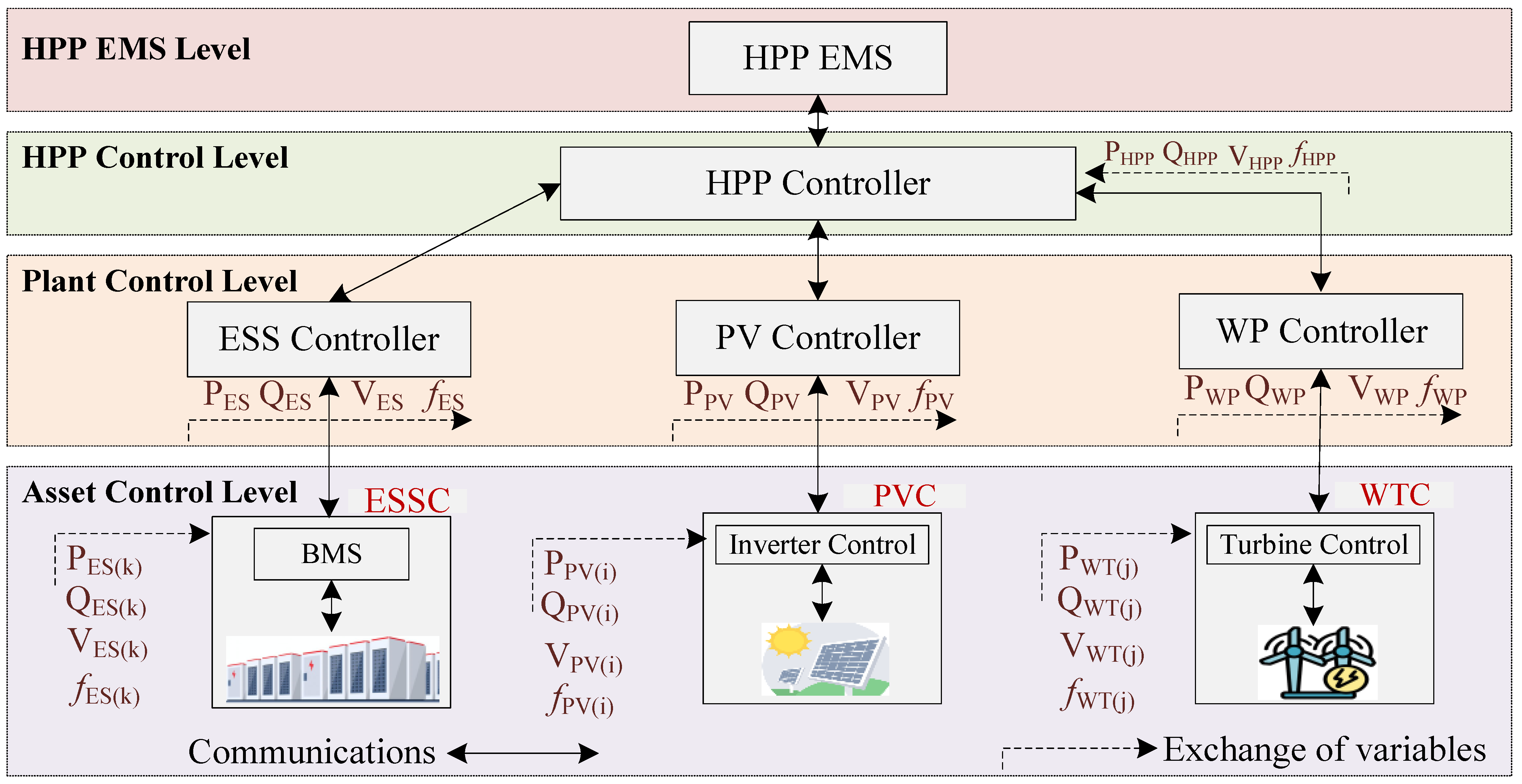
2.1. Description of the HPP Environment

The proposed HPP environment is modelled on the IEEE 14 bus network using a dynamic simulation environment. The HPP environment is comprised of 14 generation sources: six PV plants, four wind plants, and four ESS plants. The capacities of the PV plants are 11.7 MW, 14.8 MW, 17.6 MW, 10.4 MW, 10.7 MW, and 12.2 MW, located at buses 1, 2, 4, 11, 8, and 14, respectively. The capacities the WP plants are 26.7 MW, 41.4 MW, 33.4 MW, and 22.8 MW, connected on buses 3, 6, 9, 7, respectively. The capacities of the ESS plants are 21.8 MWh, 25.75 MWh, 18.6 MWh, and 22.7 MWh, located on buses 5, 12, 13, and 10, respectively. The reserve margins are set to 20% according to the maximum capacities of the PV, WP, and ESS plants. A detailed description of the HPP environment is provided in Section 4.1, where the physical parameters are listed in the nomenclature.

2.2. Objective Function

This study aims to maintain frequency stability via optimal dispatch of active power, mitigation of frequency deviation, optimisation of the reserve margin, and improvements to the power sharing capabilities of the HPP environment, as presented in Equation (1):

$$\begin{array}{c}\hfill F=\{{\beta }_1\left|P_{\mathrm{HP}}-P_{{\mathrm{HP}}_{\mathrm{ref}}}\right|+{\beta }_2\left|f_{\mathrm{HP}}-f_{{\mathrm{HP}}_{\mathrm{ref}}}\right|+{\beta }_3\left(R_{\mathrm{PV}}+R_{\mathrm{WP}}+R_{\mathrm{ESS}}\right)+\\ \hfill {\beta }_4\left|P_{\mathrm{PV}}^r+P_{\mathrm{WP}}^r+P_{\mathrm{ESS}}^r-P_{\mathrm{HP}}\right|\}\end{array}$$

(1)

where ${\beta }_1$, ${\beta }_2$, ${\beta }_3$, ${\beta }_4$ are the weighting factors, which are dynamically set for the frequency stability, while $P_{\mathrm{HP}}-P_{{\mathrm{HP}}_{\mathrm{ref}}}$, $f_{\mathrm{HP}}-f_{{\mathrm{HP}}_{\mathrm{ref}}}$, $R_{\mathrm{PV}}+R_{\mathrm{WP}}+R_{\mathrm{ESS}}$, and $P_{\mathrm{PV}}^r+P_{\mathrm{WP}}^r+P_{\mathrm{ESS}}^r-P_{\mathrm{HP}}$ are the power imbalance, frequency deviation, reserve management, and power balancing, respectively.

2.3. Constraints

For optimal dispatch and frequency stability, the following constraints must be considered [8].

2.3.1. Curtailment of PV and WP Plant

For integration and coordination of the PV and WP plants, the power capacity should not exceed the threshold for stability of the HPP, as presented below.

$$P_{\mathrm{PV}}^c=\left\{\begin{array}{cc}{P}_{\mathrm{PV}}\hfill & \mathrm{if}{P}_{\mathrm{HP}}\le P_{{\mathrm{HP}}_{\max }}\hfill \\ P_{\mathrm{PV}}-(1-\alpha )(P_{\mathrm{HP}}-P_{{\mathrm{HP}}_{\max }})\hfill & \mathrm{if}{P}_{\mathrm{HP}}>P_{{\mathrm{HP}}_{\max }}\hfill \end{array}\right.$$

(2)

$$P_{\mathrm{WP}}^c=\left\{\begin{array}{cc}{P}_{\mathrm{WP}}\hfill & \mathrm{if}{P}_{\mathrm{HP}}\le P_{{\mathrm{HP}}_{\max }}\hfill \\ P_{\mathrm{WP}}-\alpha (P_{\mathrm{HP}}-P_{{\mathrm{HP}}_{\max }})\hfill & \mathrm{if}{P}_{\mathrm{HP}}>P_{{\mathrm{HP}}_{\max }}\hfill \end{array}\right.$$

(3)

In Equations (2) and (3), $P_{\mathrm{HP}}\le P_{{\mathrm{HP}}_{\max }}$ shows no curtailment and $P_{\mathrm{HP}}>P_{{\mathrm{HP}}_{\max }}$ represents curtailment, while $\alpha$ = 1 indicates curtailment of the WP plant and $\alpha$ = 0 curtailment of the PV plant. The purpose of choosing a binary $\alpha$ is to simplify interoperability and partitioning for PV and WP agents in the proposed environment, which helps to ensure availability and prioritisation. Implementation of a continuous $\alpha$, which shows the proportional curtailment of PV and WP was not considered in this environment.

2.3.2. Power Balancing of the ESS Plant

The ESS plant provides power balancing capabilities by charging during excess power generation and discharging under low power generation, as described in Equation (4):

$$P_{\mathrm{ESS}}^c=\left\{\begin{array}{cc}{P}_{{\mathrm{ESS}}_{\min }}\hfill & \mathrm{if}{P}_{\mathrm{HP}}-P_{\mathrm{WP}}^r-P_{\mathrm{PV}}^r\le P_{{\mathrm{ESS}}_{\min }}\hfill \\ P_{{\mathrm{ESS}}_{\max }}\hfill & \mathrm{if}{P}_{\mathrm{HP}}-P_{\mathrm{WP}}^r-P_{\mathrm{PV}}^r\ge P_{{\mathrm{ESS}}_{\max }}\hfill \\ P_{\mathrm{HP}}-P_{\mathrm{WP}}^r-P_{\mathrm{PV}}^r\hfill & \mathrm{otherwise}\hfill \end{array}\right.$$

(4)

In Equation (4), $P_{\mathrm{HP}}-P_{\mathrm{WP}}^r-P_{\mathrm{PV}}^r\le P_{{\mathrm{ESS}}_{\min }}$ is the maximum discharging rate, $P_{\mathrm{HP}}-P_{\mathrm{WP}}^r-P_{\mathrm{PV}}^r\ge P_{{\mathrm{ESS}}_{\max }}$ is the maximum charging rate, and $P_{\mathrm{HP}}-P_{\mathrm{WP}}^r-P_{\mathrm{PV}}^r$ represents the dynamically adjusted charging and discharging rates. It is worth mentioning that the economic costs of ESS operation, such as cycle penalties, state-of-health (SoH), and degradation cost, are not considered in this constraint. Our proposed N—MADRL model is fully performance-oriented, and as such does not include the costs associated with operation.

2.3.3. Energy Storage at ESS Plant

The optimal energy storage at ESS plant with capacity limits is presented in Equation (5):

$$E_{{\mathrm{ESS}}_{\min }}\le E_{\mathrm{ESS}}\le E_{{\mathrm{ESS}}_{\max }}.$$

(5)

2.3.4. Frequency Control

Frequency regulation in the HPP plant ensures safe limits, helping to avoid under-frequency and over-frequency conditions by coordinating curtailments while dynamically adjusting ESS charging and inertial support, as shown in Equation (6):

$$f_{{\mathrm{HP}}_{\min }}\le f_{\mathrm{HP}}\le f_{{\mathrm{HP}}_{\max }}.$$

(6)

The proposed constraints are specific for optimal dispatch and frequency control, while the inverter dynamics, such as voltage and current loops, are not considered in the N—MADRL environment. Thus, the reward is entirely performance-based for optimal dispatch and frequency regulation objectives. In addition, the problem of maintaining frequency stability via optimally dispatching active power, mitigating frequency deviation, optimising reserve management, and improving power sharing capabilities is presented for real-time HPP grid conditions. The optimisation problem is formulated by considering the actual HPP environment, its dynamic behaviour, uncertainties in HPP assets, and the decentralised coordination of multi-agent control of the HPP environment. Conventional optimisation control schemes, such as MPC and rule-based schemes, require a centralised control environment, leading to challenges around scalability, performance, coordination, and adaptability. To address these limitations, the N—MADRL framework proposed in this research provides a decentralised, adaptive, scalable, and coordinated approach for providing frequency-control ancillary services in HPP environments.

3. Proposed Networked Multi-Agent Deep Reinforcement Learning (N—MADRL) Approach

This section addresses the network representation of N—MADRL to develop a decentralised coordination control network for the HPP environment. The preliminaries of MADRL presented in this section are used for learning policies according to states, actions, observations, rewards, and the transition state of N—MADRL agents in the environment. The control policies of the N—MADRL framework are presented using the MASAC approach, which combines MAAC and SAC schemes. The scalability and heterogeneity issues of N—MADRL are addressed and developed through decentralised control functions. At the end of this section, the implementation of N—MADRL is presented using current and target value functions.

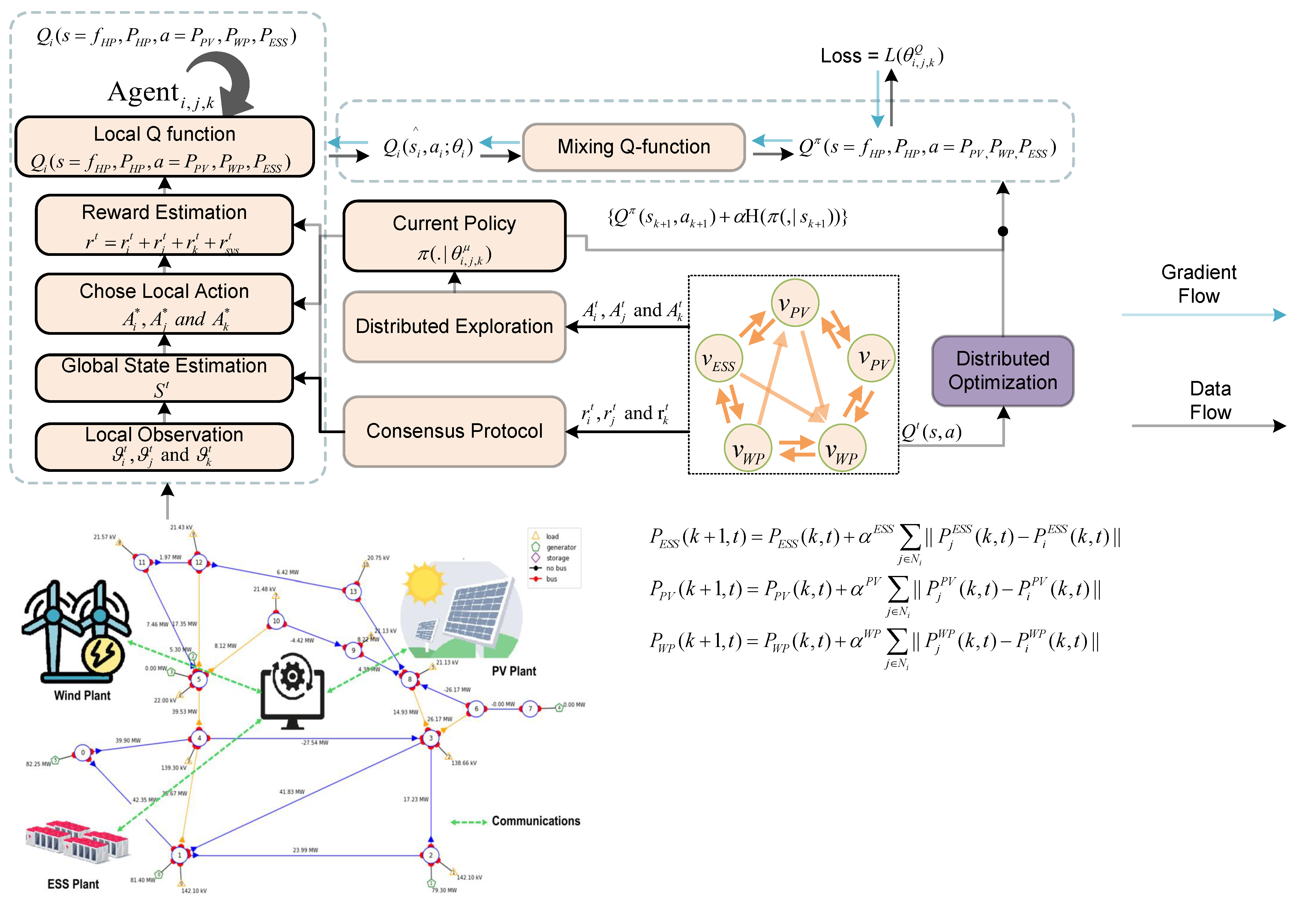
3.1. Network Representation

In a conventional power network, grid operators use centralised control for power balancing and frequency regulation. Today, due to the increasing penetration of IBR-enabled resources, centralised control is changing to decentralised control to meet scalability, computational, and optimal performance requirements. In addition, the complexity of centralised control networks can be reduced by decentralised control systems thanks to their ability to independently and autonomously operate power network resources. As our proposed HPP network is an IBR-enabled power system, we used the N—MADRL framework for frequency-control ancillary services. In the proposed N—MADRL framework, a decentralised network of HPP resources is coordinated using multi-agent control, placing each resource within a collaborative learning environment for frequency regulation and power balancing. In the proposed N—MADRL framework, each resource is considered as an independent agent coordinating with corresponding agents to create a multi-agent environment. The decision-making process of a multi-agent control environment involves learning and executing without the need for centralised control systems.

To shape the centralised control operation within a decentralised model, our proposed HPP environment is divided into three zones for the PV, WP, and ESS plants; each zone has a decentralised topology for interacting with neighbouring plants. Let the HPP environment be represented by the graph $\mathcal{G}$, which contains agents $\mathcal{V}$ and $\mathcal{E}$ for communication, i.e., $\mathcal{G}=\{\mathcal{V},\mathcal{E}\}$. The number of PV, WP, and ESS agents are ${\mathcal{N}}_{\mathrm{P}\mathrm{V}}$, ${\mathcal{N}}_{\mathrm{W}\mathrm{P}}$, and ${\mathcal{N}}_{\mathrm{E}\mathrm{S}\mathrm{S}}$, respectively. The assets of each zone are ${\mathcal{N}}_{\mathrm{P}\mathrm{V}}={\mathcal{N}}_{\mathrm{p}\mathrm{v}\mathrm{1}}\dots ,{\mathcal{N}}_{\mathrm{p}\mathrm{v}\mathrm{n}}$, ${\mathcal{N}}_{\mathrm{W}\mathrm{P}}={\mathcal{N}}_{\mathrm{w}\mathrm{p}\mathrm{1}}\dots ,{\mathcal{N}}_{\mathrm{w}\mathrm{p}\mathrm{n}}$, and ${\mathcal{N}}_{\mathrm{E}\mathrm{S}\mathrm{S}}={\mathcal{N}}_{\mathrm{e}\mathrm{s}\mathrm{s}\mathrm{1}}\dots ,{\mathcal{N}}_{\mathrm{e}\mathrm{s}\mathrm{s}\mathrm{n}}$, respectively. The agents are connected with $\mathcal{G}=\{{\mathcal{V}}_{\mathrm{PV}},{\mathcal{V}}_{\mathrm{WP}},{\mathcal{V}}_{\mathrm{ESS}},\mathcal{E}\}$ using $\mathcal{E}\subset {\mathcal{V}}_{\mathrm{PV}}\times {\mathcal{V}}_{\mathrm{WP}}\times {\mathcal{V}}_{\mathrm{ESS}}$. The total number of HPP agents ${\mathcal{V}}_{\mathrm{HPP}}$ is ${\mathcal{V}}_{\mathrm{PV}}+{\mathcal{V}}_{\mathrm{WP}}+{\mathcal{V}}_{\mathrm{ESS}}$. The adjacency matrix is ${\mathcal{A}}_{\mathrm{ij}}=\left[1\right]$ for adjacent agents and ${\mathcal{A}}_{\mathrm{ij}}=\left[0\right]$ for non-adjacent agents. The degree matrix ${\mathcal{D}}_{\mathrm{ij}}=diag[{\mathcal{D}}_{\mathrm{ij}}\dots ,{\mathcal{D}}_{\mathrm{n}}$] shows the number of connections, while the Laplacian matrix $\left[{\mathcal{L}}_{\mathrm{ij}}\right]=\left[{\mathcal{D}}_{\mathrm{ij}}\right]-[{\mathcal{A}}_{\mathrm{ij}}$] shows the connected agents. The Laplacian matrix ${\mathcal{L}}_{\mathrm{ij}}$ of the networked graph is shown below.

$${\mathcal{L}}_{\mathrm{ij}}=\left\{\begin{array}{cc}-1\hfill & \mathrm{if}j\in {\mathcal{N}}_{\mathcal{i}}\hfill \\ |{\mathcal{N}}_i|\hfill & \mathrm{if}j=i\hfill \end{array}\right.$$

(7)

3.2. MADRL Preliminaries

For the MADRL network of the HPP environment, a Markov decision process (MDP) is used for learning policies according to their states, actions, observations, rewards, and the global state of the agents [46]. For a given time t, the MDP is represented with five tuples: $\left\{\mathcal{N},{\mathcal{S}}^t,{\mathcal{A}}^t,{\mathcal{O}}^t\right.$, $\left.{\mathcal{R}}^t\right\}$, where $\mathcal{N}=\{1,2,\dots ,n\}$ is the number of agents, ${\mathcal{S}}^t$ is the global state, the action of the agent is ${\mathcal{A}}^t=\left\{a_1,a_2,a_3,\dots ,a_n\right\}$, the observation of the agent is ${\mathcal{O}}^t=\left\{o_1,o_2,o_3,\dots ,o_n\right\}$, and the reward $\mathcal{R}$ is ${\mathcal{R}}_i:\left({\mathcal{S}}^t\times \{r_1,r_2,r_3,\dots ,r_n\}\right)\mapsto {\mathcal{R}}^t$. Each agent chooses an action based on its observation, which is called policy mapping: ${\pi }_i:{\mathcal{S}}_i\mapsto \mathcal{P}\left({\mathcal{A}}_i\right)$. After the agent executes action ${\mathcal{A}}^t$, it receives an immediate reward $r_i^t:\left({\mathcal{S}}_i^t\times {\mathcal{A}}_i^t\right)\mapsto {\mathcal{R}}^t$ and proceeds to the next state $\mathcal{P}\left({\mathcal{S}}^{t+1}\mid {\mathcal{S}}^t,{\mathcal{A}}^t\right)$. Then, the agent observes new states and performs actions based on the new observations: $\mathcal{P}\left({\mathcal{O}}_i^{t+1}\mid {\mathcal{S}}^t\right)$. This process is continued until the optimal policy ${\pi }_i^{*}$: ${\pi }_1,{\pi }_2,{\pi }_3,\dots ,{\pi }_n$ is maximised, as follows:

$$M\left({\pi }_i^{*}\right)=\underset{{\pi }_i}{max}\underset{\begin{array}{c}{a}_i^t\sim {\pi }_i\end{array}}{\mathbb{R}}\left[\sum _{t=0}^t{\gamma }^t{r}_i^t\right]$$

(8)

where $M\left({\pi }_i^{*}\right)$ is the expected return from optimal policy and ${\gamma }^t$ is the discounted factor $\gamma \in [0,1]$ used to estimate immediate and long-term future rewards.

In addition, a state-value function represented by $V^t\left(s\right)$ is used to maximise the policy returns for optimal dispatch and frequency stability. The action-value function is represented by $Q^t(s,a)$, which performs optimal actions in specific states for optimal dispatch and frequency stability. The state-value and action-value functions of agents are represented as follows:

$$\begin{array}{c}\hfill V_i(s=f_{\mathrm{HP}},P_{\mathrm{HP}})=\underset{{\pi }_i}{max}\underset{\begin{array}{c}{a}_i^t\sim {\pi }_i\end{array}}{\mathbb{E}}\left[\sum _{t=0}^T{\gamma }^t{r}_i^t\mid s=f_{\mathrm{HP}},P_{\mathrm{HP}}\right],\end{array}$$

(9)

$$\begin{array}{c}\hfill Q_i(s=f_{\mathrm{HP}},P_{\mathrm{HP}},a=P_{\mathrm{PV}},P_{\mathrm{WP}},P_{\mathrm{ESS}})=\underset{{\pi }_i}{max}\underset{\begin{array}{c}{a}_i^t\sim {\pi }_i\end{array}}{\mathbb{E}}\sum _{t=0}^T{\gamma }^t{r}_i^t(s=f_{\mathrm{HP}},P_{\mathrm{HP}},a=P_{\mathrm{PV}},P_{\mathrm{WP}},P_{\mathrm{ESS}}).\end{array}$$

(10)

In the N—MADRL scheme, agents only use a partially observable Markov game (POMG) [40] for the system state ${\mathcal{S}}^t$$\left\{P_{\mathrm{HP}},P_{\mathrm{PV}}^r,P_{\mathrm{WP}}^r,P_{\mathrm{ESS}}^r\right\}$. Observations ${\mathcal{O}}_i^t$, ${\mathcal{O}}_j^t$, ${\mathcal{O}}_k^t$ for action ${\mathcal{A}}^t$ of agents $i,j,k$ at time t are represented as ${\mathcal{A}}_i^t$, ${\mathcal{A}}_j^t$, ${\mathcal{A}}_k^t$ for $\{-l,l\}$, where l is the range of optimal dispatch and reserve management. In addition, every agent interacts only with a neighbouring agent in PV, WP, and ESS zones. The states and observations of agents are limited to their zones, meaning that they do not contribute to global agents in the global space. In this way, the POMG is represented as follows:

• Agents: Agents $i,j,k$ represent PV, WP, and ESS assets, respectively.
• Region Set: The HPP environment is considered in terms of PV, WP, and ESS zones.
• System States: The system state ${\mathcal{S}}^t$ contains the global information set of all agents, for instance $\left\{P_{\mathrm{HP}},P_{\mathrm{PV}}^r,P_{\mathrm{WP}}^r,P_{\mathrm{ESS}}^r\right\}$.
• Agent Observation: The observation sets of PV, WP, and ESS agents are ${\mathcal{O}}_i^t$, ${\mathcal{O}}_j^t$, ${\mathcal{O}}_k^t$, respectively.
• Agent Actions: An action ${\mathcal{A}}^t$ of agent $i,j,k$ at time t is represented as ${\mathcal{A}}_i^t:-l\le {\mathcal{A}}_i^t\le l$, ${\mathcal{A}}_j^t:-l\le {\mathcal{A}}_j^t\le l$, and ${\mathcal{A}}_k^t:-l\le {\mathcal{A}}_k^t\le l$, representing the optimal dispatch and frequency control. The boundary of ${\mathcal{A}}_i^t$, ${\mathcal{A}}_j^t$, and ${\mathcal{A}}_k^t$ is limited within $\{-l,l\}$, where l represents optimal dispatch and reserve management.
• Reward Function: For optimal dispatch and frequency stability, the shared reward function $r_{hpp}^t$ accumulates the system reward $r_{sys}^t$ and agent reward $r_{pv}^t+r_{wp}^t+r_{ess}^t$, formulated as follows:

$$\begin{array}{c}\hfill r_{sys}^t=-{\beta }_1\left|P_{\mathrm{HP}}-P_{{\mathrm{HP}}_{\mathrm{ref}}}\right|-{\beta }_2\left|f_{\mathrm{HP}}-f_{{\mathrm{HP}}_{\mathrm{ref}}}\right|+\\ \hfill {\beta }_3\left(R_{\mathrm{PV}}+R_{\mathrm{WP}}+R_{\mathrm{ESS}}\right)+{\beta }_4\left|P_{\mathrm{PV}}^r+P_{\mathrm{WP}}^r+P_{\mathrm{ESS}}^r-P_{\mathrm{HP}}\right|\end{array}$$

(11)

where $P_{\mathrm{HP}}-P_{{\mathrm{HP}}_{\mathrm{ref}}}$ and $f_{\mathrm{HP}}-f_{{\mathrm{HP}}_{\mathrm{ref}}}$ are negative rewards, while $R_{\mathrm{PV}}+R_{\mathrm{WP}}+R_{\mathrm{ESS}}$ and $P_{\mathrm{PV}}^r+P_{\mathrm{WP}}^r+P_{\mathrm{ESS}}^r-P_{\mathrm{HP}}$ are positive rewards. The agent rewards are formulated on power balancing, energy reserve, and frequency control, as follows:

$$r_{\mathrm{pv}}^t=-\left\{{\alpha }_1\left|P_{\mathrm{pv}}^r-P_{{\mathrm{pv}}_{\mathrm{ref}}}\right|+{\alpha }_2\left|f_{\mathrm{HP}}-f_{{\mathrm{HP}}_{\mathrm{ref}}}\right|+{\alpha }_3{R}_{\mathrm{pv}}\right\},$$

(12)

$$r_{\mathrm{wp}}^t=-\left\{{\omega }_1\left|P_{\mathrm{wp}}^r-P_{{\mathrm{wp}}_{\mathrm{ref}}}\right|+{\omega }_2\left|f_{\mathrm{HP}}-f_{{\mathrm{HP}}_{\mathrm{ref}}}\right|+{\omega }_3{R}_{\mathrm{wp}}\right\},$$

(13)

$$r_{\mathrm{ess}}^t=-\left\{{\sigma }_1\left|P_{\mathrm{ess}}^r-P_{{\mathrm{ess}}_{\mathrm{ref}}}\right|+{\sigma }_2\left|f_{\mathrm{HP}}-f_{{\mathrm{HP}}_{\mathrm{ref}}}\right|+{\sigma }_3{R}_{\mathrm{ess}}\right\}.$$

(14)

The evaluation of reward coefficients is aligned with optimal dispatch and frequency stability. Thus, weights ${\beta }_1$, ${\alpha }_1$, ${\omega }_1$, and ${\sigma }_1$ are two to three times greater than the remaining weights. The optimisation of these weights is focused on the N—MADRL model to develop performance-based rewards [54]. This approach prioritises grid stability and frequency regulation, as opposed to the cost optimisation in [14], which focused on minimising cost despite compromising grid performance. The shared reward of the N—MADRL scheme for the HPP environment is

$$r_{hpp}^t=r_{\mathrm{sys}}^t+r_{\mathrm{pv}}^t+r_{\mathrm{wp}}^t+r_{\mathrm{ess}}^t.$$

(15)

State Transitions: When PV, WP, or ESS agents execute actions ${\mathcal{A}}_i^t$, ${\mathcal{A}}_j^t$, and ${\mathcal{A}}_k^t$ under states ${\mathcal{S}}_i^t$, ${\mathcal{S}}_j^t$, and ${\mathcal{S}}_k^t$, the transition function moves the environment to new states ${\mathcal{S}}_i^{t+1}$, ${\mathcal{S}}_j^{t+1}$, and ${\mathcal{S}}_k^{t+1}$. As the transition functions of the agents are unknown within the environment, the proposed N—MADRL approach chooses an optimal policy for the HPP agents. The optimal policy ${\pi }_i^{*}$: ${\pi }_1,{\pi }_2,{\pi }_3,\dots ,{\pi }_n$ maximises the expected values before completion of the transition function.

3.3. Multi-Agent and Soft Actor–Critic (MASAC) Approach

In the multi-agent actor-critic (MAAC) approach, the actor selects actions to maximise the current rewards, while the critic selects actions for the actor to maximise expected future rewards. Referring to Equations (9) and (10), the value functions $V_i(s=f_{\mathrm{HP}},P_{\mathrm{HP}})$ and $Q_i(s=f_{\mathrm{HP}},P_{\mathrm{HP}},a=P_{\mathrm{PV}},P_{\mathrm{WP}},P_{\mathrm{ESS}})$ are optimised for the state–action context. Agent ${\mathcal{V}}_{\mathrm{PV}},{\mathcal{V}}_{\mathrm{WP}},{\mathcal{V}}_{\mathrm{ESS}}$ contains decentralised actors that use local states $P_{\mathrm{PV}},P_{\mathrm{WP}},P_{\mathrm{ESS}}$ in policy ${\pi }_i^{*}$. For optimal dispatch and frequency control, this provides optimal results for the actor loss and critic loss as well as fast convergence and an optimal learning process that maximises rewards. Through global observation of the critic network, it provides optimal actions ${\mathcal{A}}_i^{*}$, ${\mathcal{A}}_j^{*}$, and ${\mathcal{A}}_k^{*}$ for the current states ${\mathcal{S}}_i^t$, ${\mathcal{S}}_j^t$, and ${\mathcal{S}}_k^t$. In testing, each agent ${\mathcal{V}}_{\mathrm{PV}},{\mathcal{V}}_{\mathrm{WP}},{\mathcal{V}}_{\mathrm{ESS}}$ for states $P_{\mathrm{PV}},P_{\mathrm{WP}},P_{\mathrm{ESS}}$ accesses its own actors for optimal actions ${\mathcal{A}}_i^{*}$, ${\mathcal{A}}_j^{*}$, and ${\mathcal{A}}_k^{*}$, ensuring operation in a decentralised fashion. As the HPP environment is a continuous action space, a soft actor-critic (SAC) scheme is integrated with MAAC to measure the entropy for the uncertainties and randomness of policy actions. Unlike DDPG and PPO schemes, SAC balances agent exploration and exploitation during training. The expected reward is updated using entropy maximisation, as follows:

$$J\left(\pi \right)=\sum _{k=0}^n{\mathbb{E}}_{(s_k,a_k)\sim \pi }\left[r(s_k,a_k)+\alpha \mathcal{H}\left(\pi (·\mid s_k)\right)\right]$$

(16)

where $\mathcal{H}\left(\pi (·\mid s_k)\right)$ is the entropy function and $\alpha$ is the stochasticity control parameter for policy optimisation. Referring to Equations (9) and (10), the expected returns are modified for the entropy-regularised functions, as follows:

$$V^{\pi }(s=f_{\mathrm{HP}},P_{\mathrm{HP}})={\mathbb{E}}_{\pi }\left[\sum _{k=0}^{\infty }{\gamma }^k\left(r_k+\alpha \mathcal{H}\left(\pi (·\mid s_k)\right)\right)\mid s_0=f_{\mathrm{HP}},P_{\mathrm{HP}}\right],$$

(17)

$$\begin{array}{c}\hfill Q^{\pi }(s=f_{\mathrm{HP}},P_{\mathrm{HP}},a=P_{\mathrm{PV}},P_{\mathrm{WP}},P_{\mathrm{ESS}})={\mathbb{E}}_{\pi }[\sum _{k=0}^{\infty }{\gamma }^k\left(r_k+\alpha \mathcal{H}\left(\pi (·\mid s_k)\right)\right)\\ \hfill |s_0=f_{\mathrm{HP}},P_{\mathrm{HP}},a_0=P_{\mathrm{PV}},P_{\mathrm{WP}},P_{\mathrm{ESS}}].\end{array}$$

(18)

The relationship between $V^{\pi }\left(s\right)$ and $Q^{\pi }(s,a)$ is expressed as follows:

$$\begin{array}{c}\hfill V^{\pi }(s=f_{\mathrm{HP}},P_{\mathrm{HP}})={\mathbb{E}}_{a\sim \pi }[Q^{\pi }(s=f_{\mathrm{HP}},P_{\mathrm{HP}},a=P_{\mathrm{PV}},P_{\mathrm{WP}},P_{\mathrm{ESS}})\\ \hfill +\alpha \mathcal{H}\left(\pi (·\mid s_k)\right)|s_0=f_{\mathrm{HP}},P_{\mathrm{HP}}].\end{array}$$

(19)

To balance the exploration process and develop a probabilistic model instead of a deterministic model, the entropy-regularised Bellman equation is used to handle a highly sampled complex HPP environment. Because the HPP environment is a probabilistic model, the entropy-regularised Bellman equation is expressed as follows:

$$\begin{array}{c}\hfill Q^{\pi }(s=f_{\mathrm{HP}},P_{\mathrm{HP}},a=P_{\mathrm{PV}},P_{\mathrm{WP}},P_{\mathrm{ESS}})={\mathbb{E}}_{\begin{array}{c}{s}_{k+1}\sim P\\ a_{k+1}\sim \pi \end{array}}[r_k+\gamma Q^{\pi }(s_{k+1},a_{k+1})\\ \hfill +\alpha \mathcal{H}\left(\pi (·\mid s_{k+1})\right)].\end{array}$$

(20)

Using Equation (20), the entropy-regularised Bellman equation is then rearranged as follows:

$$\begin{array}{c}\hfill Q^{\pi }(s=f_{\mathrm{HP}},P_{\mathrm{HP}},a=P_{\mathrm{PV}},P_{\mathrm{WP}},P_{\mathrm{ESS}})=\\ \hfill {\mathbb{E}}_{s_{k+1}\sim P}\left[r_k+\gamma V^{\pi }(s_{k+1}=f_{\mathrm{HP}},P_{\mathrm{HP}})\right].\end{array}$$

(21)

The policy in the HPP environment is improved and updated at every k iteration for the value functions $V^{\pi }\left(s\right)$ and $Q^{\pi }(s,a)$.

3.4. Scalability and Heterogeneity

As the HPP environment includes PV, WP, and ESS assets with different capacities, control functions, and operating zones, the networked approach of the MADRL model meets the need for scalability and heterogeneity of agents. Let the state of agents ${\mathcal{V}}_{\mathrm{HPP}}$, ${\mathcal{V}}_{\mathrm{PV}},{\mathcal{V}}_{\mathrm{WP}},{\mathcal{V}}_{\mathrm{ESS}}$ be $P_{\mathrm{HP}},P_{\mathrm{PV}},P_{\mathrm{WP}},P_{\mathrm{ESS}}$ such that $P_{\mathrm{HP}}=P_{\mathrm{PV}}+P_{\mathrm{WP}}+P_{\mathrm{ESS}}$ using Equations (2)–(4). Similarly, the frequencies using Equation (6) are $f_{\mathrm{PV}}$, $f_{\mathrm{WP}}$, $f_{\mathrm{ESS}}$, $f_{\mathrm{HP}}$. The initial states $P_{\mathrm{PV}},P_{\mathrm{WP}},P_{\mathrm{ESS}}$ and $f_{\mathrm{PV}}$, $f_{\mathrm{WP}}$, $f_{\mathrm{ESS}}$ after k iterations are updated with a control input $U_{ij}$, as shown below.

$$\left[\begin{array}{c}{P}_{\mathrm{PV}}(k+1)\\ P_{\mathrm{WP}}(k+1)\\ P_{\mathrm{ESS}}(k+1)\\ P_{\mathrm{HP}}(k+1)\end{array}\right]=\left[\begin{array}{c}{P}_{\mathrm{PV}}\left(k\right)\\ P_{\mathrm{WP}}\left(k\right)\\ P_{\mathrm{ESS}}\left(k\right)\\ P_{\mathrm{HP}}\left(k\right)\end{array}\right]+\left[\begin{array}{c}{U}_{ij}^{\mathrm{pv}}\left(k\right)\\ U_{ij}^{\mathrm{wp}}\left(k\right)\\ U_{ij}^{\mathrm{ess}}\left(k\right)\\ U_{ij}^{\mathrm{hpp}}\left(k\right)\end{array}\right]$$

(22)

$$\left[\begin{array}{c}{f}_{\mathrm{PV}}(k+1)\\ f_{\mathrm{WP}}(k+1)\\ f_{\mathrm{ESS}}(k+1)\\ f_{\mathrm{HP}}(k+1)\end{array}\right]=\left[\begin{array}{c}{f}_{\mathrm{PV}}\left(k\right)\\ f_{\mathrm{WP}}\left(k\right)\\ f_{\mathrm{ESS}}\left(k\right)\\ f_{\mathrm{HP}}\left(k\right)\end{array}\right]+\left[\begin{array}{c}{U}_{ij}^{\mathrm{pv}}\left(k\right)\\ U_{ij}^{\mathrm{wp}}\left(k\right)\\ U_{ij}^{\mathrm{ess}}\left(k\right)\\ U_{ij}^{\mathrm{hpp}}\left(k\right)\end{array}\right]$$

(23)

Referring to the Equation (22) for active power states and Equation (23) for frequency control, the control input is $U_{\mathrm{ij}}^{\mathrm{pv}}$, $U_{\mathrm{ij}}^{\mathrm{wp}}$, $U_{\mathrm{ij}}^{\mathrm{ess}}$, which after coordination with neighbour agents becomes $U_{\mathrm{ij}}^{\mathrm{pv}}={\sum }_{j\in {\mathcal{N}}_i}\parallel P_{\mathrm{j}}^{\mathrm{pv}}-P_{\mathrm{i}}^{\mathrm{pv}}\parallel$, $U_{\mathrm{ij}}^{\mathrm{wp}}={\sum }_{j\in {\mathcal{N}}_i}\parallel P_{\mathrm{j}}^{\mathrm{wp}}-P_{\mathrm{i}}^{\mathrm{wp}}\parallel$, $U_{\mathrm{ij}}^{\mathrm{ess}}={\sum }_{j\in {\mathcal{N}}_i}\parallel P_{\mathrm{j}}^{\mathrm{ess}}-P_{\mathrm{i}}^{\mathrm{ess}}\parallel$. The updated Equation (22) is then:

$$P_{\mathrm{PV}}(k+1)=P_{\mathrm{PV}}\left(k\right)+{\alpha }^{\mathrm{pv}}\sum _{j\in {\mathcal{N}}_i}\parallel P_{\mathrm{j}}^{\mathrm{pv}}\left(k\right)-P_{\mathrm{i}}^{\mathrm{pv}}\left(k\right)\parallel ,$$

(24)

$$P_{\mathrm{WP}}(k+1)=P_{\mathrm{WP}}\left(k\right)+{\alpha }^{\mathrm{wp}}\sum _{j\in {\mathcal{N}}_i}\parallel P_{\mathrm{j}}^{\mathrm{wp}}\left(k\right)-P_{\mathrm{i}}^{\mathrm{wp}}\left(k\right)\parallel ,$$

(25)

$$P_{\mathrm{ESS}}(k+1)=P_{\mathrm{ESS}}\left(k\right)+{\alpha }^{\mathrm{ess}}\sum _{j\in {\mathcal{N}}_i}\parallel P_{\mathrm{j}}^{\mathrm{ess}}\left(k\right)-P_{\mathrm{i}}^{\mathrm{ess}}\left(k\right)\parallel .$$

(26)

The convergence factors ${\alpha }^{\mathrm{pv}},{\alpha }^{\mathrm{wp}},{\alpha }^{\mathrm{ess}}$ ranging from 0–1 represent the speed of convergence in decentralised coordination and assess the stability in communication resiliency. Based on sensitivity analysis and optimal convergence, the lowest value of ${\alpha }^{\mathrm{pv}},{\alpha }^{\mathrm{wp}},{\alpha }^{\mathrm{ess}}$ demonstrates the slowest convergence, while the highest values of ${\alpha }^{\mathrm{pv}},{\alpha }^{\mathrm{wp}},{\alpha }^{\mathrm{ess}}$ accelerate the convergence process. In our proposed N—MADRL environment, the range of ${\alpha }^{\mathrm{pv}},{\alpha }^{\mathrm{wp}},{\alpha }^{\mathrm{ess}}$ is kept dynamic for the PV, WP, and ESS zones to assess the communication resiliency in dynamically changing topologies along with the speed of decentralised coordination. The combined convergence factors are expressed as follows:

$$\alpha ={\displaystyle \frac{1}{\mathcal{N}}}({\alpha }^{\mathrm{pv}}\sum _i{P}_{\mathrm{PV}}+{\alpha }^{\mathrm{wp}}\sum _j{P}_{\mathrm{WP}}+{\alpha }^{\mathrm{ess}}\sum _k{P}_{\mathrm{ESS}}).$$

(27)

The resiliency of the N—MADRL scheme is evaluated by considering communication failures under the dynamic topologies in the HPP environment, as shown in Figure 2. For the time-varying t dynamic topology, the control inputs for the PV, WP, and ESS agents are $U_{\mathrm{ij},\mathrm{t}}^{\mathrm{pv}}$, $U_{\mathrm{ij},\mathrm{t}}^{\mathrm{wp}}$, $U_{\mathrm{ij},\mathrm{t}}^{\mathrm{ess}}$, respectively. Now, the PV, WP, and ESS agents exchange their control inputs $U_{\mathrm{ij},\mathrm{t}}^{\mathrm{pv}}$ with neighbour agents $U_{\mathrm{ij},\mathrm{t}}^{\mathrm{pv}}={\sum }_{j\in {\mathcal{N}}_i}\parallel P_{\mathrm{j},\mathrm{t}}^{\mathrm{pv}}-P_{\mathrm{i},\mathrm{t}}^{\mathrm{pv}}\parallel$, $U_{\mathrm{ij},\mathrm{t}}^{\mathrm{wp}}={\sum }_{j\in {\mathcal{N}}_i}\parallel P_{\mathrm{j},\mathrm{t}}^{\mathrm{wp}}-P_{\mathrm{i},\mathrm{t}}^{\mathrm{wp}}\parallel$, $U_{\mathrm{ij},\mathrm{t}}^{\mathrm{ess}}={\sum }_{j\in {\mathcal{N}}_i}\parallel P_{\mathrm{j},\mathrm{t}}^{\mathrm{ess}}-P_{\mathrm{i},\mathrm{t}}^{\mathrm{ess}}\parallel$, respectively. In this way, the control functions and training of heterogeneous agents under the dynamic topology are redeveloped, and Equations (24)–(26) are updated as follows:

$$\begin{array}{c}\hfill P_{\mathrm{PV}}(k+1,t)=P_{\mathrm{PV}}(k,t)+{\alpha }^{\mathrm{pv}}\sum _{j\in {\mathcal{N}}_i}\parallel P_{\mathrm{j}}^{\mathrm{pv}}(k,t)-P_{\mathrm{i}}^{\mathrm{pv}}(k,t)\parallel ,\end{array}$$

(28)

$$\begin{array}{c}\hfill P_{\mathrm{WP}}(k+1,t)=P_{\mathrm{WP}}(k,t)+{\alpha }^{\mathrm{wp}}\sum _{j\in {\mathcal{N}}_i}\parallel P_{\mathrm{j}}^{\mathrm{wp}}(k,t)-P_{\mathrm{i}}^{\mathrm{wp}}(k,t)\parallel ,\end{array}$$

(29)

$$\begin{array}{c}\hfill P_{\mathrm{ESS}}(k+1,t)=P_{\mathrm{ESS}}(k,t)+{\alpha }^{\mathrm{ess}}\sum _{j\in {\mathcal{N}}_i}\parallel P_{\mathrm{j}}^{\mathrm{ess}}(k,t)-P_{\mathrm{i}}^{\mathrm{ess}}(k,t)\parallel .\end{array}$$

(30)

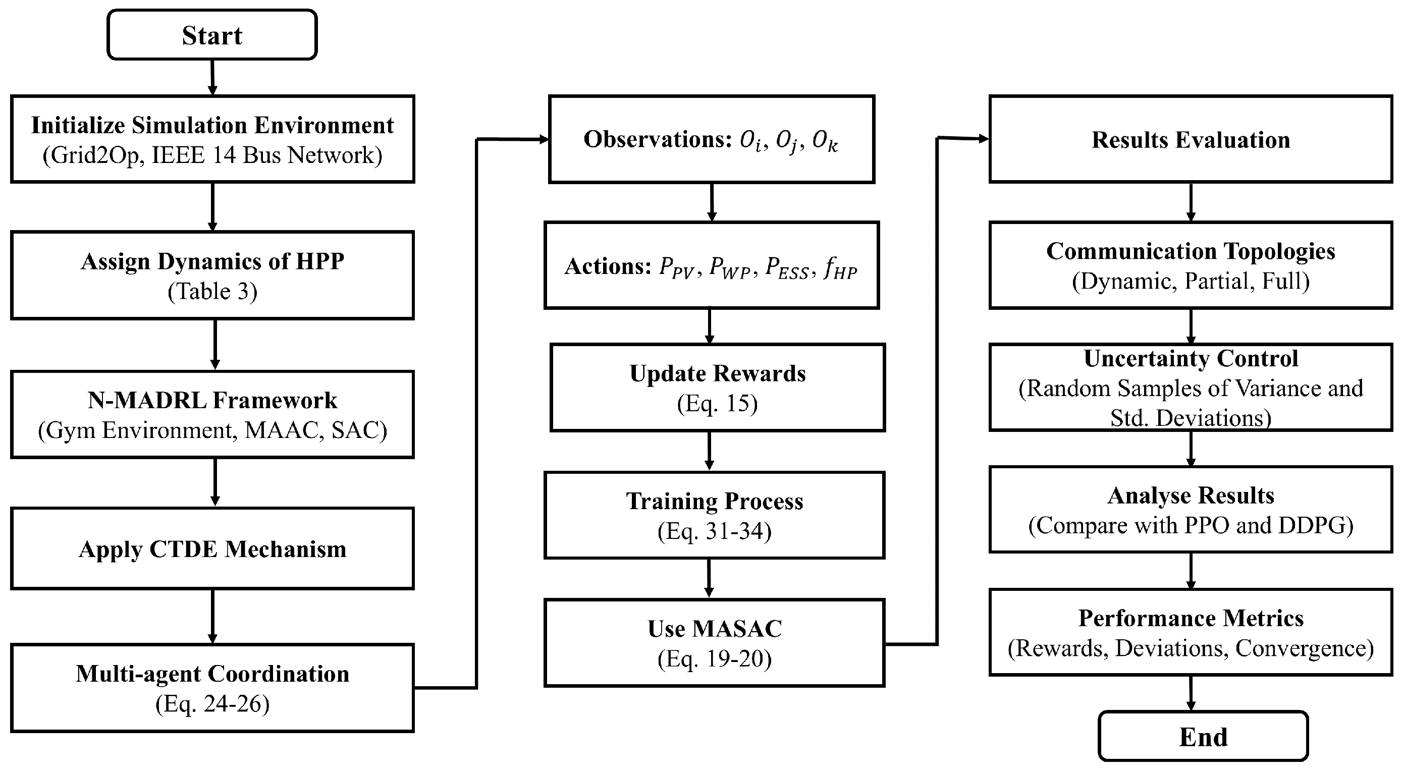
3.5. N—MADRL Implementation

The detailed illustration of the N—MADRL approach is presented in Figure 3. The current value network is a Q-value network in the training process, which minimises the difference between the predicted and target values of Q functions. Similarly, the target value network is the stabilised version of the current value network, which helps to mitigate training instability and divergence. As the HPP environment is nonstationary for PV, WP, and ESS assets, the control policy for each agent is dependent and requires optimal coordination. The N—MADRL scheme uses a centralised critic network and a decentralised actor network for optimal training of the HPP environment. It uses decentralised actors for the collective action and observation of PV, WP, and ESS assets ${\mathcal{C}}_k^{pv}=\{o_1^k\dots ,o_n^k,a_1^k\dots ,a_n^k\mid {\theta }_i^Q\}$, ${\mathcal{C}}_k^{wp}=\{o_1^k,\dots ,o_n^k,a_1^k,\dots ,a_n^k\}\mid {\theta }_j^Q\}$, and ${\mathcal{C}}_k^{ess}=\{o_1^k,\dots ,o_n^k,a_1^k,\dots ,a_n^k\mid {\theta }_k^Q\}\}$, respectively. Then, the critic network estimates Q-values $Q^{\pi }(s=f_{\mathrm{HP}},P_{\mathrm{HP}},a=P_{\mathrm{PV}},P_{\mathrm{WP}},P_{\mathrm{ESS}})$ using centralised training. For states $P_{\mathrm{PV}},P_{\mathrm{WP}},P_{\mathrm{ESS}}$, we access their actors for actions ${\mathcal{A}}_i^{*}=\mu (o_i^k\mid {\theta }_i^{\mu })$, ${\mathcal{A}}_j^{*}=\mu (o_j^k\mid {\theta }_j^{\mu })$, and ${\mathcal{A}}_k^{*}=\mu (o_k^k\mid {\theta }_k^{\mu })$ in decentralised fashion, which requires observation of each agent. The proposed Q-value and target value functions are formulated as follows:

$$L\left({\theta }_{i,j,k}^Q\right)={\mathbb{E}}_{(o^k,a^k,s^{k+1},r^k)\sim \mathcal{D}}\left[\left({(y_{\mathrm{pv}}^k-{\mathcal{C}}_k^{\mathrm{pv}})}^2+{(y_{\mathrm{wp}}^k-{\mathcal{C}}_k^{\mathrm{wp}})}^2+{(y_{\mathrm{ess}}^k-{\mathcal{C}}_k^{\mathrm{ess}})}^2\right)\right],$$

(31)

$$y_{i,j,k}^t=r_{hpp}^t+\gamma \left\{Q^{\pi }(s_{k+1},a_{k+1})+\alpha \mathcal{H}\left(\pi (·\mid s_{k+1})\right)\right\}.$$

(32)

Here, $L\left({\theta }_{i,j,k}^Q\right)$ is the loss function, ${\mathcal{C}}_{i,j,k}$ are the parameters for the Q functions, and $y_{i,j,k}^t$ are the target values of the HPP agents. Because the reward and inputs in critic networks differ in the HPP environment, the control policy in the learning and training process is customised for the PV, WP, and ESS agents. Therefore, we compared the proposed algorithm with the on-policy PPO algorithm and off-policy DDPG algorithm for learning the optimal policy, maximising the reward, and improving the policy. The proposed policy gradient is formulated as follows:

$${\nabla }_{{\theta }_{i,j,k}^{\mu }}\mathcal{J}\approx {\mathbb{E}}_{o^k\sim \mathcal{D}}\left[\{{\nabla }_{a_i,a_j,a_k}{Q}^{\pi }(s_{k+1},a_{k+1})+\alpha \mathcal{H}\left(\pi (·\mid s_{k+1})\right)\}{\nabla }_{{\theta }_{i,j,k}^{\mu }}\mu (o_{i,j,k}\mid {\theta }_{i,j,k}^{\mu })\right].$$

(33)

For training stabilization, the target ${\theta }_{i,j,k}^{\prime }$ and expected ${\nabla }_{{\theta }_{i,j,k}^{\mu }}\mathcal{J}$ values are expressed as

$${\theta }_{i,j,k}^{\prime }\leftarrow {\theta }_{i,j,k}+\tau {\nabla }_{{\theta }_{i,j,k}^{\mu }}\mathcal{J}.$$

(34)

Soft updating of the target value network ${\theta }_{i,j,k}^{\prime }$ uses expected value network ${\nabla }_{{\theta }_{i,j,k}^{\mu }}\mathcal{J}$, with $\tau$ indicating the learning rate. This gradually updates the target network to prevent instability in the learning process. The N—MADRL scheme is explained in Algorithm 1; for actors of PV, WP, ESS agents, the actions are ${\mathcal{A}}_i^k$, ${\mathcal{A}}_j^k$, ${\mathcal{A}}_k^k$, respectively. Observations $o_i^k$, $o_j^k$, and $o_k^k$ are retrieved in accordance with state information $s_i^k$, $s_j^k$, and $s_k^k$ using the current policy $\pi (·\mid {\theta }_{i,j,k}^{\mu })$ for cumulative rewards $r_{hpp}^t$ and the next state observations $o_i^{k+1}$, $o_j^{k+1}$, and $o_k^{k+1}$ stored in the replay buffer $\mathcal{D}$. To accelerate the training process, samples from the PV, WP, and ESS agents are segmented in mini-batches $\mathcal{B}\left(\mathcal{D}\right)$ in the replay buffer. The training process in the N—MADRL approach has $\mathcal{M}$ episodes and $\mathcal{T}$ steps. The training process continues until the PV, WP, and ESS agents in the HPP environment converge for optimal dispatch, reserve maximisation, and frequency control.

Algorithm 1 Proposed N—MADRL Scheme

1: Initialize environment and agent parameters.   2: for each agent $\mathcal{N}=\{1,2,\dots ,n\}$ do   3:     Initialise parameters for the current critic-actor and target actor-critic networks.   4:     Initialize control actions ${\theta }_{i,j,k}^{\mu }$ of agent $i,j,k$.   5:     Initialize control actions in PV, WP, and ESS zones: ${\theta }_i^{\mu }$, ${\theta }_j^{\mu }$, and ${\theta }_k^{\mu }$.   6: end for   7: for each episode $m=1$ to $\mathcal{M}$ do   8:     Initialize CTDE for exploration of HPP environment.   9:     Receive initial observations ${\mathcal{O}}_i^t$, ${\mathcal{O}}_j^t$, ${\mathcal{O}}_k^t$ for PV, WP, and ESS zones. 10:     Store observations in replay buffer $\mathcal{D}$. 11:     for each time step $t=1$ to $\mathcal{T}$ do 12:         Select actions: ${\mathcal{A}}_i^{*}=\mu (o_i^t\mid {\theta }_i^{\mu })$, ${\mathcal{A}}_j^{*}=\mu (o_j^t\mid {\theta }_j^{\mu })$, ${\mathcal{A}}_k^{*}=\mu (o_k^t\mid {\theta }_k^{\mu })$. 13:         Execute observations and actions: ${\mathcal{C}}_k^{pv}$, ${\mathcal{C}}_k^{wp}$, ${\mathcal{C}}_k^{ess}$ for PV, WP, and ESS agents. 14:         for each agent $i,j,k=1$ to ${\mathcal{N}}_{\mathrm{PV}},{\mathcal{N}}_{\mathrm{WP}},{\mathcal{N}}_{\mathrm{ESS}}$ do 15:            Store tuples in replay buffer $\mathcal{D}$: ${\mathcal{S}}_i^t,{\mathcal{S}}_j^t,{\mathcal{S}}_k^t$ (states), ${\mathcal{A}}_i^t,{\mathcal{A}}_j^t,{\mathcal{A}}_k^t$ (actions), $r_{hpp}^t$ (reward), ${\mathcal{S}}_i^{t+1},{\mathcal{S}}_j^{t+1},{\mathcal{S}}_k^{t+1}$ (new states). 16:         end for 17:         if $\mathcal{D}$ is full then 18:            for each agent $i,j,k=1$ to ${\mathcal{N}}_{\mathrm{PV}},{\mathcal{N}}_{\mathrm{WP}},{\mathcal{N}}_{\mathrm{ESS}}$ do 19:                Store tuples in replay buffer $\mathcal{D}$ again. 20:                Update actor weights in current value network: $L\left({\theta }_{i,j,k}^Q\right)$. 21:                Update critic weights in current value network: $L\left({\theta }_{i,j,k}^Q\right)$. 22:                Update actor weights in target value network: $y_{i,j,k}^t$. 23:                Update critic weights in target value network: $y_{i,j,k}^t$. 24:                Update policy gradient: ${\nabla }_{{\theta }_{i,j,k}^{\mu }}\mathcal{J}$. 25:            end for 26:            Update target value network for PV, WP, and ESS agents: ${\theta }_{i,j,k}^{\prime }\leftarrow {\theta }_{i,j,k}+\tau {\nabla }_{{\theta }_{i,j,k}^{\mu }}\mathcal{J}$. 27:         end if 28:     end for 29: end for 30: Repeat until convergence.

The detailed flowchart of the proposed N—MADRL framework is presented in Figure 4. The N—MADRL framework initiates agents in the Grid2Op environment of the HPP power system. Each HPP source is modelled as an independent agent in three zones of the IEEE 14 bus network. Multi-agent interaction is initiated using episodic steps by observing the HPP environment using time steps. The optimal actions for dispatch and frequency control are executed to obtain episodic rewards and HPP environment global rewards. Reward maximisation is conducted using the continuous action state and the experience samples stored in the replay buffer. For optimal memory management, the buffer is segmented into mini-batches and checked for the convergence of proposed learning policies. When the replay buffer is full, the convergence of N—MADRL policies for optimal dispatch and frequency control is evaluated. Otherwise, the process is initiated again to update the actor-critic network of MASAC until convergence occurs. Meanwhile, the updated target values network is consistently associated with the convergence parameter. This looping process is continuous until the experience samples are collected and stored in the replay buffer and fully associate the target network with the value network for learning the control policies for optimal dispatch and frequency control. This process occurs in a centralised fashion among the three zones of the HPP environment during the training process. In the execution stage, the decentralised control policies are tested and exercised in order to assess optimal dispatch, reserve management, power imbalance, and active power sharing.

4. Numerical Simulations

In this section, the proposed N—MADRL environment is explained through the Grid2Op dynamic simulation environment and its control parameters. The results of training and learning control policies are evaluated and compared with DRL algorithms. The optimal dispatch analysis is presented for dynamically changing, partially-connected, and fully-connected communication topologies.

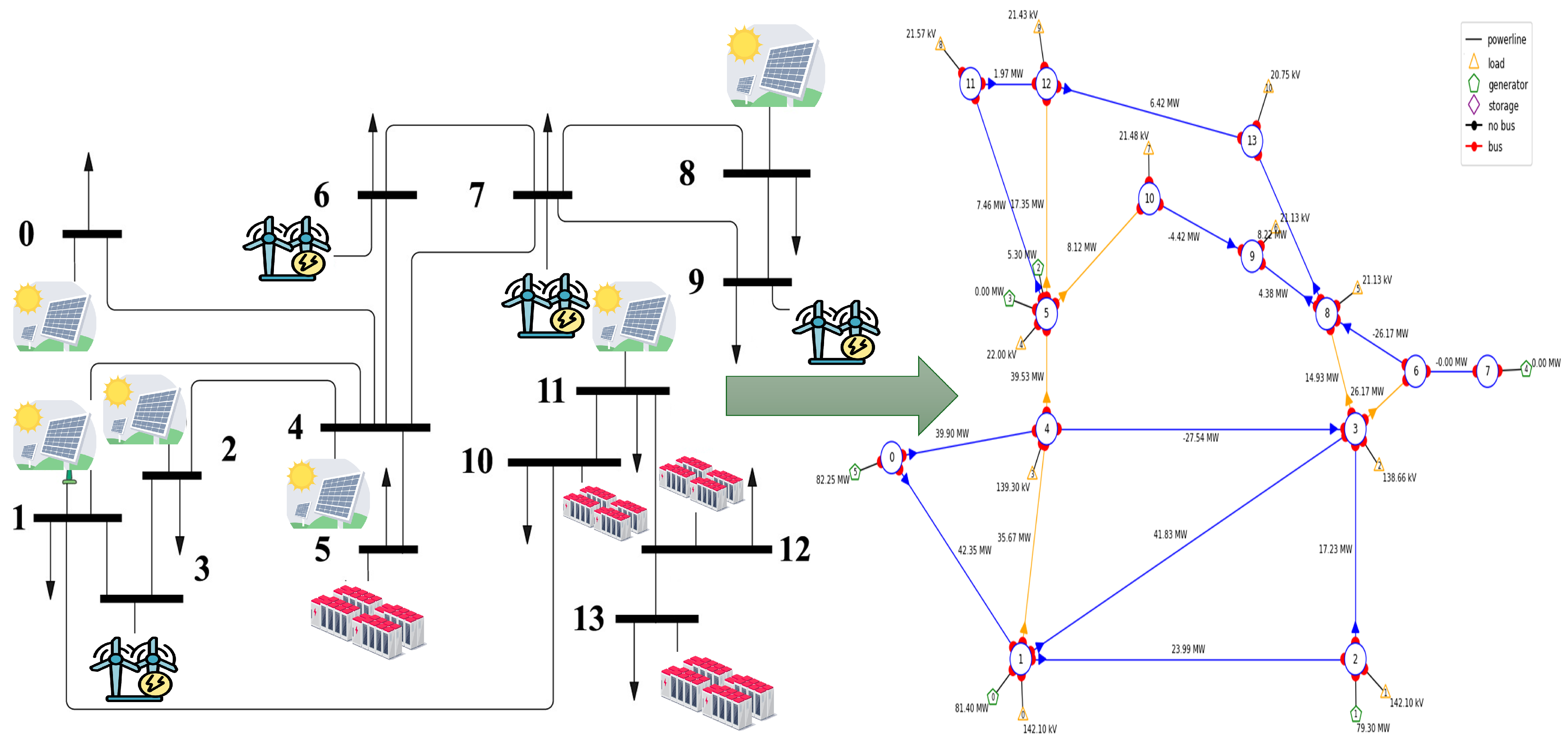
4.1. N—MADRL Environment

Simulations of the N—MADRL model were conducted on a computer with 64-bit Windows 10 OS, Core i7 station, 2.50 GHz processor, and 16 GB RAM. The N—MADRL model was developed in Python framework using a gymnasium environment and implementing numerous DRL algorithms such as MAAC and SAC. The simulations of HPP power systems were executed in the Grid2Op dynamic simulation environment [55].

Table 2. Parameter settings for DRL algorithms.

Algorithms	Parameters	Values
N—MADRL	Actors hidden units	{128, 256}
	Actors hidden layers	{2, 5}
	Critic hidden units	{128, 256}
	Critic hidden layers	{2, 5}
	Learning rate	0.0003
	${\alpha }^{\mathrm{pv}},{\alpha }^{\mathrm{wp}},{\alpha }^{\mathrm{ess}}$	0.60
PPO & DDPG	Actors hidden units	256
	Critic hidden units	256
	Optimizer	Adam
	Activation function	ReLU
Shared	Learning rate	0.0003
	Mini-batch size $\mathcal{M}$	64
	Reply buffer $\mathcal{D}$	${10}^6$
	Discount factor ${\gamma }^t$	0.97
	Total iterations k	${10}^6$
	Soft update $\tau$	0.10

shows the parameter selection of the N—MADRL, PPO, and DDPG algorithms.

The flowchart for the numerical simulations of the N—MADRL framework is illustrated in Figure 5 for training, validation, and evaluation of the HPP environment. The initialisation of the HPP model in the Grid2Op environment was started using the IEEE 14 bus system. The Grid2Op environment was associated with the N—MADRL framework by using the CDTE mechanism for agent interactions and exchanging control inputs. Decentralised coordination among the PV, WP, and ESS plants was initiated by observing the respective states and taking the appropriate actions for optimal dispatch and frequency deviation control. This process continued until maximising the N—MADRL shared reward functions for the HPP environment. To stabilise the learning and control policies, the MASAC approach was implemented in the training process to observe the attention and entropy regularisation of the N—MADRL environment. The results were evaluated for dynamic, partially-connected, and fully-connected communication topologies to asses the training stability. In addition, random samples were initiated in the training samples to observe uncertainty control by assessing variance and standard deviations. The results of the proposed N—MADRL framework were compared with those of the PPO and DDPG DRL algorithms for optimal dispatch and frequency control. In addition, the performance metrics were evaluated for N—MADRL, PPO, and DDPG to observe the cumulative rewards, frequency deviations, and convergence rates in the HPP environment.

As the objective and constraints are not formulated in a static optimisation case, it was integrated with the Grid2Op dynamic simulation environment using the N—MADRL control scheme. In this scenario, the multi-agent controllers interact with dynamically changing frequency due to the imbalances of the HPP environment resources. The process of learning policies of the N—MADRL framework captures nonlinear frequency from Grid2Op to provide realistic grid conditions. The Grid2Op dynamic simulation environment supports time domain system states, action-based multi-agent interactions, and communication contingencies. For the Grid2Op dynamic simulation environment, the proposed N—MADRL approach implemented centralised training and decentralised execution using integrated MAAC and SAC algorithms for the optimal dispatch of multi-agent controllers. The nonlinearity of frequency in the Grid2Op environment is demonstrated by considering physical constraints of the HPP environment, Grid2Op simulation network effects, and nonlinear mapping decisions of optimal dispatch actions.

Figure 6 depicts IEEE 14 bus HPP systems with the distribution of PV, WP, and ESS plants, 19 transmission lines, and 14 generation sources.

Table 3. The dynamics of the PV, WP, and ESS plants in the HPP environment.

g-id	Bus	Asset	${\mathit{U}}_{\mathbf{ij}}^{\mathbf{pv}}$	${\mathit{U}}_{\mathbf{ij}}^{\mathbf{wp}}$	${\mathit{U}}_{\mathbf{ij}}^{\mathbf{ess}}$	${\mathit{P}}_{\mathbf{PV}}^{\mathit{c}}$	${\mathit{P}}_{\mathbf{WP}}^{\mathit{c}}$	${\mathit{P}}_{\mathbf{ESS}}^{\mathit{c}}$	${\mathit{R}}_{\mathbf{PV}}$	${\mathit{R}}_{\mathbf{WP}}$	${\mathit{R}}_{\mathbf{ESS}}$
0	1	pv	0.039	0	0	11.7	0	0	2.34	0	0
1	5	ess	0	0	0.032	0	0	21.8	0	0	4.36
2	3	wind	0	0.026	0	0	26.7	0	0	5.34	0
3	12	ess	0	0	0.030	0	0	25.75	0	0	5.15
4	2	pv	0.036	0	0	14.8	0	0	2.96	0	0
5	6	wind	0	0.023	0	0	41.4	0	0	8.28	0
6	4	pv	0.034	0	0	17.6	0	0	3.52	0	0
7	13	ess	0	0	0.029	0	0	18.6	0	0	3.72
8	9	wind	0	0.025	0	0	33.4	0	0	6.68	0
9	11	pv	0.037	0	0	10.4	0	0	2.08	0	0
10	7	wind	0	0.021	0	0	22.8	0	0	4.56	0
11	10	ess	0	0	0.031	0	0	22.7	0	0	4.54
12	8	pv	0.035	0	0	10.7	0	0	2.14	0	0
13	14	pv	0.038	0	0	12.2	0	0	2.44	0	0

refers to the dynamics of the $P_{\mathrm{PV}}$, $P_{\mathrm{WP}}$, $P_{\mathrm{ESS}}$ HPP environment in the Grid2Op simulations. In the Grid2Op simulations, the PV, WP, and ESS plants participate in optimal dispatch, reserve management, and frequency control services. Specifically, six PV plants with capacities of 11.7 MW, 14.8 MW, 17.6 MW, 10.4 MW, 10.7 MW, and 12.2 MW are connected on buses 1, 2, 4, 11, 8, and 14, respectively. In addition, four WP plants are connected to buses 3, 6, 9, and 7, with capacities of 26.7 MW, 41.4 MW, 33.4 MW, and 22.8 MW, respectively. Similarly, the four ESS plants have capacities of 21.8 MWh, 25.75 MWh, 18.6 MWh, and 22.7 MWh and are connected on buses 5, 12, 13, and 10, respectively. The $P_{\mathrm{PV}}$, $P_{\mathrm{WP}}$, $P_{\mathrm{ESS}}$ data were simulated on dynamic, partially-connected, and fully-connected communication topologies. The algorithm parameters were configured from the gymnasium environment and stable baseline3 DRL algorithms, while the $P_{\mathrm{PV}}$, $P_{\mathrm{WP}}$, $P_{\mathrm{ESS}}$ characteristics were programmed using the Grid2Op simulation platform with the reserve margins set to 20% according to the maximum capacities of the PV, WP, and ESS plants.

4.2. Results Validation

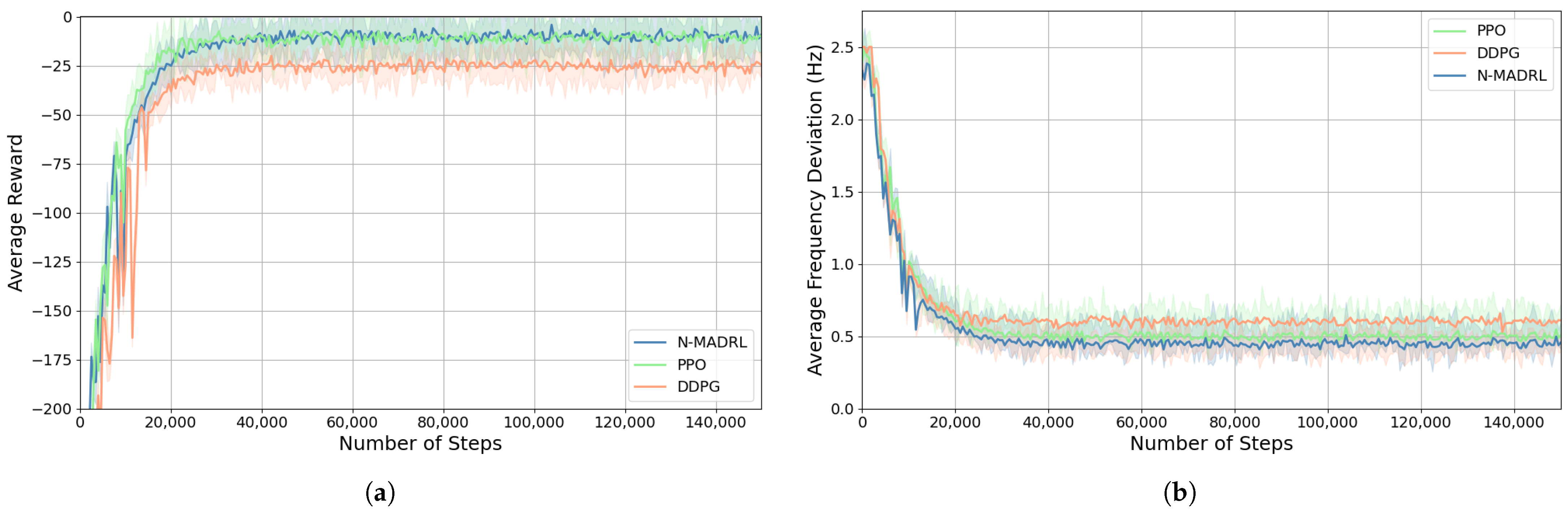
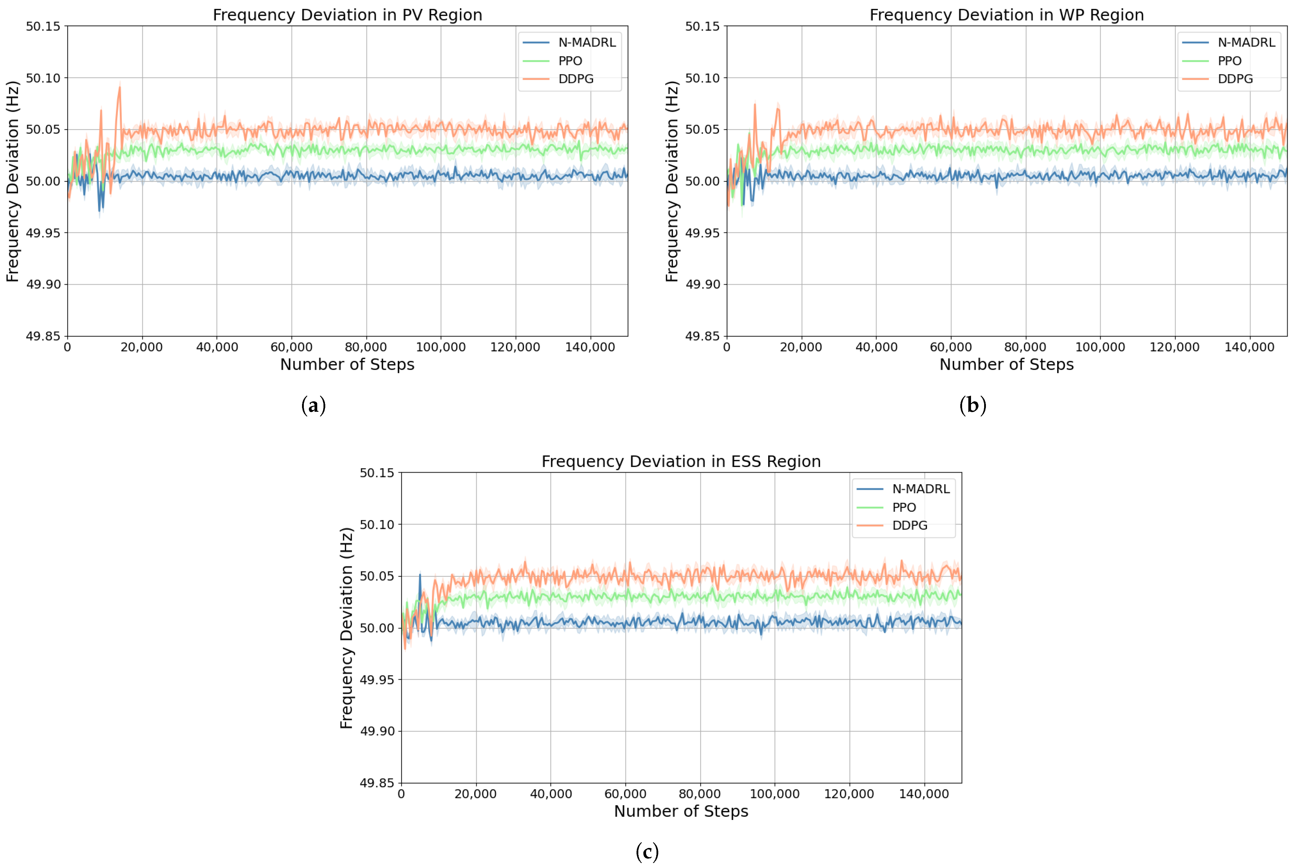
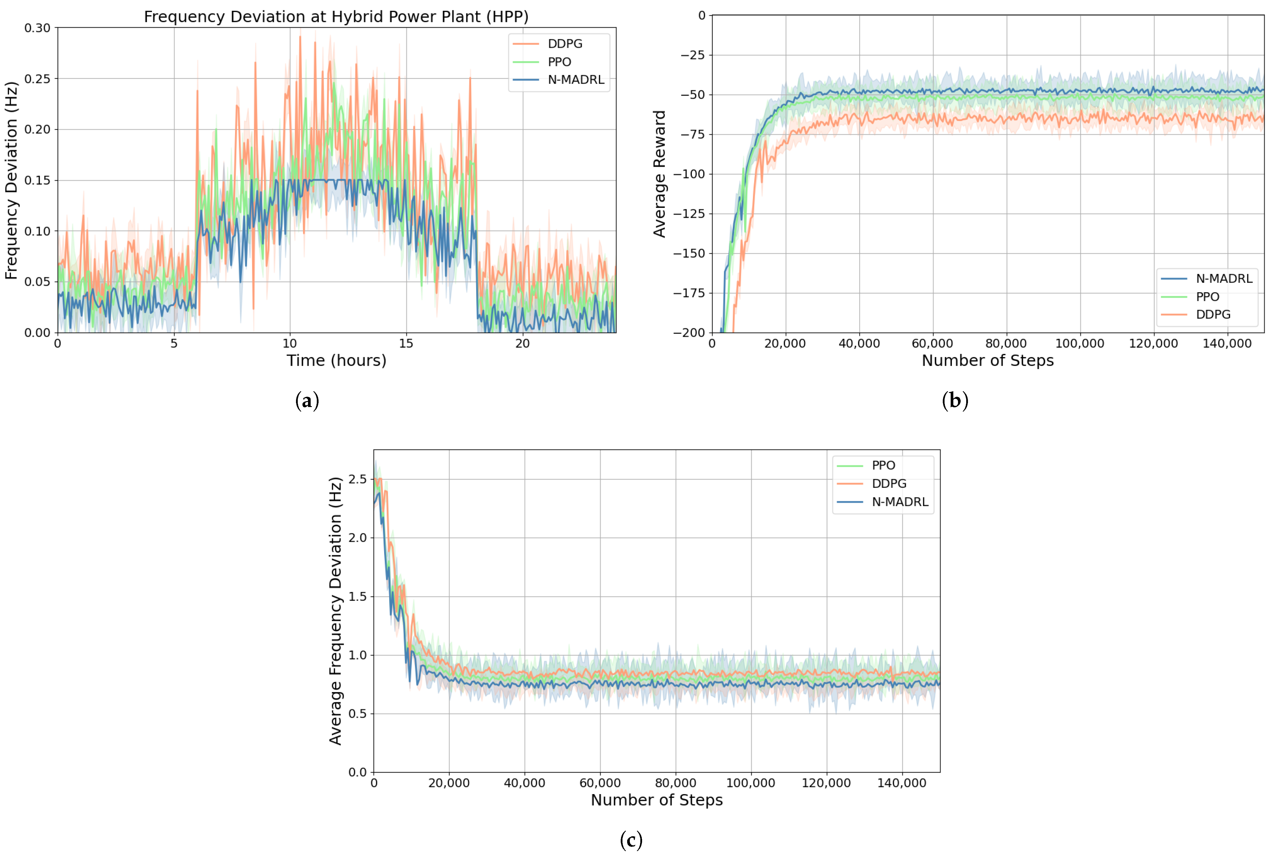
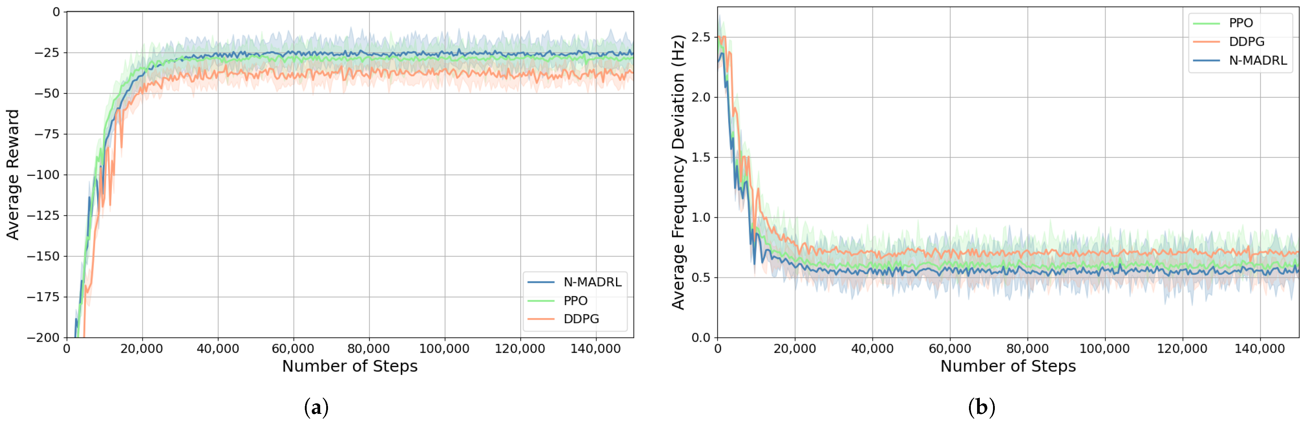
4.2.1. Training Process

For effective generalisation, the data were partitioned into 80% training, 10% validation, and 10% testing datasets. The training dataset was used to optimise the policy network, the validation dataset for tuning the hyperparameters, and the testing dataset for assessing the model’s ability to generalise. In addition, the robustness of the proposed model was evaluated by implementing random five-fold cross-validation, in which four folds were used for training and one fold for validation in each iteration.

The training process of the N—MADRL scheme was benchmarked with continuous action-space DRL algorithms such as DDPG and PPO. The DDPG offers off-policy actor-critic and deterministic policy gradients for handling continuous action-space data in the HPP environment, which helps to optimise active power dispatch for frequency control and complex decision-making. In contrast, PPO is an on-policy policy gradient algorithm that implements a method for balancing exploration and exploitation, making for a stable training process. In addition, PPO helps to minimise frequency deviations in a complex HPP environment. Moreover, both schemes use actor-critic frameworks, cooperative control, and uncertainty management to address such complex environments.

The performance of the DDPG and PPO algorithms compared to N—MADRL was evaluated using localised training and execution. In contrast, N—MADRL achieved optimal performance using centralised training and decentralised execution (CTDE) for optimal dispatch and frequency stability. Figure 7 shows the cumulative rewards and frequency deviations in the training processes of the N—MADRL, DDPG, and PPO algorithms. In Figure 7, the solid lines show the average values of random experiments and the error margins are represented with shaded lines.

Initially, the HPP agents did not stabilise the frequencies among HPP assets due to the unknown environment and limited agent interactions. The cumulative rewards were maximised and the frequency deviations reduced as the training progressed. The N—MADRL approach presented higher performance than DDPG and PPO, dispatching an average power of 0.22 MW with an average frequency deviation of 0.013 Hz. This superior performance is due to its partial observability, attention mechanism, and nonstationary behaviour. In contrast, PPO provided an average power dispatch of 0.38 MW with a frequency deviation of 0.041 Hz, while DDPG offered an average power dispatch of 0.57 MW with an average frequency deviation of 0.053 Hz. The variance in PPO’s convergence is due to its stochastic behaviour and limited exploration within the highly dynamic HPP environment. PPO offers clipping behaviour to avoid instabilities, but is not able to control large variances. The instabilities in the performance of PPO are due to Gaussian distribution samples in the highly dynamic POMG HPP environment. In addition, PPO utilises only new samples and does not use samples from experience, ultimately resulting in policy shifts. On the other hand, N—MADRL uses centralised critic and entropy regularisation, which enhances its performance, helping it to achieve 42.10% and 61.40% more efficiency in optimal dispatch than PPO and DDPG, respectively. In terms of frequency stability, N—MADRL is more stable than PPO and DDPG, achieving improvements of 68.30% and 74.48%, respectively.

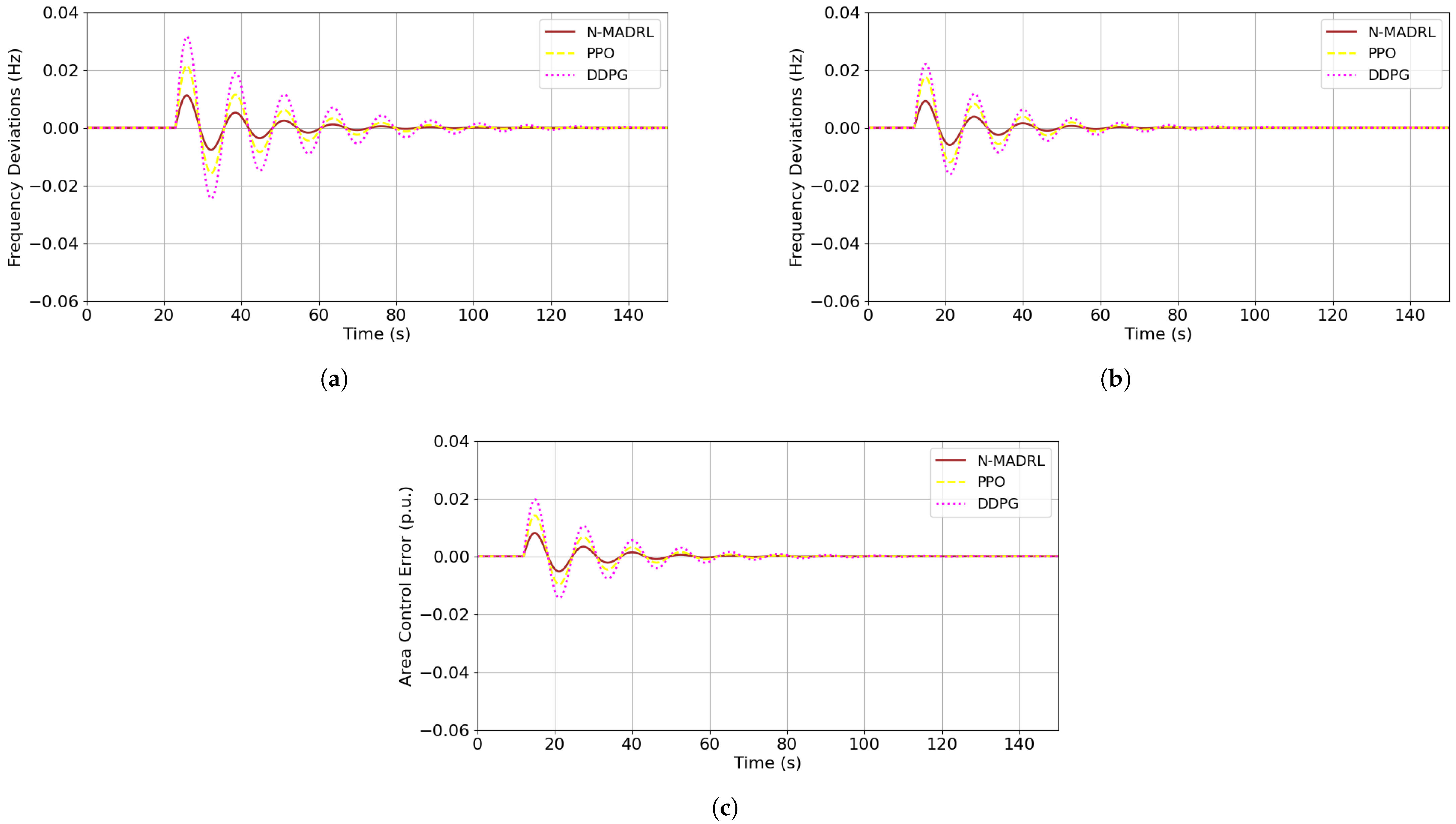
4.2.2. Comparison of DRL Algorithms

To validate the performance of the proposed N—MADRL scheme in comparison with other DRL schemes, a peak generation scenario was considered in which optimal dispatch and frequency deviation pose a challenging issue.

Table 4. Computational cost comparison of the N—MADRL, PPO, and DDPG algorithms.

Algorithms	Training (hr)	Validation (min)	Testing (min)
N—MADRL	6.50	25	13
PPO	8.25	40	21
DDPG	10.20	50	24

provides a computational cost comparison of the N—MADRL, PPO, and DDPG algorithms in terms of training, validation, and testing times. It shows that the computational cost of N—MADRL for training is lower than that of PPO and DDPG despite the complex architecture incorporating MAAC and SAC. In addition, the validation and testing results of N—MADRL are higher than those of PPO and DDPG, proving its robust convergence and computational efficiency. These results provide validation for and practical deployment of real-world HPP environments. The DDPG algorithm uses a replay buffer in centralised training in the actor–critic network to store $o_i^k$, $o_j^k$, $o_k^k$ for states $s_i^k$, $s_j^k$, $s_k^k$, using the current policy $\pi (·\mid {\theta }_{i,j,k}^{\mu })$ for rewards $r_{hpp}^t$ and the next state $s_i^{k+1}$, $s_j^{k+1}$, $s_k^{k+1}$ without using additional centralised training of the HPP environment. In contrast, N—MADRL performs execution solely on local states and operates independently for PV, WP, ESS assets based on $P_{\mathrm{PV}}$, $P_{\mathrm{WP}}$, $P_{\mathrm{ESS}}$ for $P_{\mathrm{HP}}$ and $f_{\mathrm{HP}}$, as shown in Figure 8a.

For the PPO scheme, the centralised training of agents is developed by using the agents’ collective data to update the proximal policy. DDPG and PPO do not use the additional centralised data of the HPP environment to optimise control performance. In addition, PPO executes stochastic policy $\pi (·\mid {\theta }_{i,j,k}^{\mu })$ using observations $o_i^k$, $o_j^k$, $o_k^k$ and states $s_i^k$, $s_j^k$, $s_k^k$ for HPP agents to estimate the accumulative reward $r_{hpp}^t$. as shown in Figure 8b.

In contrast, N—MADRL uses an MAAC scheme as an attention mechanism for the heterogeneous agents $P_{\mathrm{PV}}$, $P_{\mathrm{WP}}$, $P_{\mathrm{ESS}}$ to estimate global states $P_{\mathrm{HP}}$ and $f_{\mathrm{HP}}$. The N—MADRL scheme uses integrated SAC ${\mathcal{C}}_{i,j,k}$ parameters for Q-value and target functions $y_{i,j,k}^t$ to minimise the loss function $L\left({\theta }_{i,j,k}^Q\right)$ and maximise accumulative rewards. As the episodic reward and input of the critic network are different at the initial stage, the training process is not mature at the beginning. Exploration and entropy maximisation $\mathcal{H}\left(\pi (·\mid s_k)\right)$ using experience samples from the replay buffer helps to maximise the reward compared to PPO and DDPG algorithms, as shown in Figure 8c.

The frequency deviations are assessed with existing and proposed optimisation schemes under the dynamic simulation environment of Grid2Op, stochastic policies of the N—MADRL learning process, and control performance of the HPP environment. It is worth noting that small frequency deviations in PV, WP, and ESS regions are due to the absence of explicit modelling parameters, the dynamic simulation environment of Grid2Op, and the N—MADRL learning process. Moreover, the control performance indicates that our proposed framework provides superior stability compared to PPO and DDPG.

Table 5. Performance comparison of the N—MADRL, PPO, and DDPG algorithms.

Algorithms	Ave. Rewards	Ave. Deviation (Hz)	Ave. Power (MW)
N—MADRL	−9.93	0.013	0.22
PPO	−12.45	0.041	0.38
DDPG	−24.58	0.053	0.57

provides the performance comparison of the N—MADRL, PPO, and DDPG algorithms.

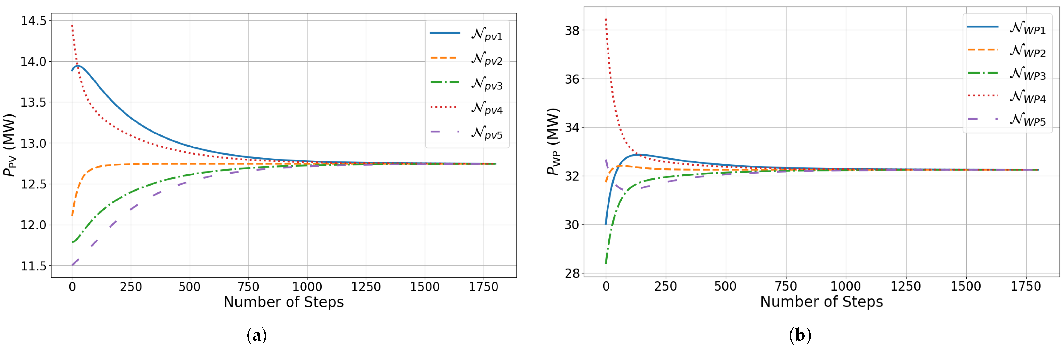
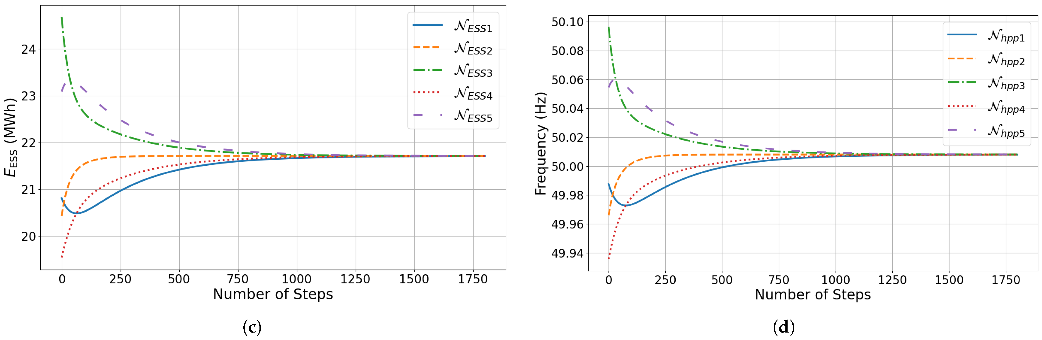
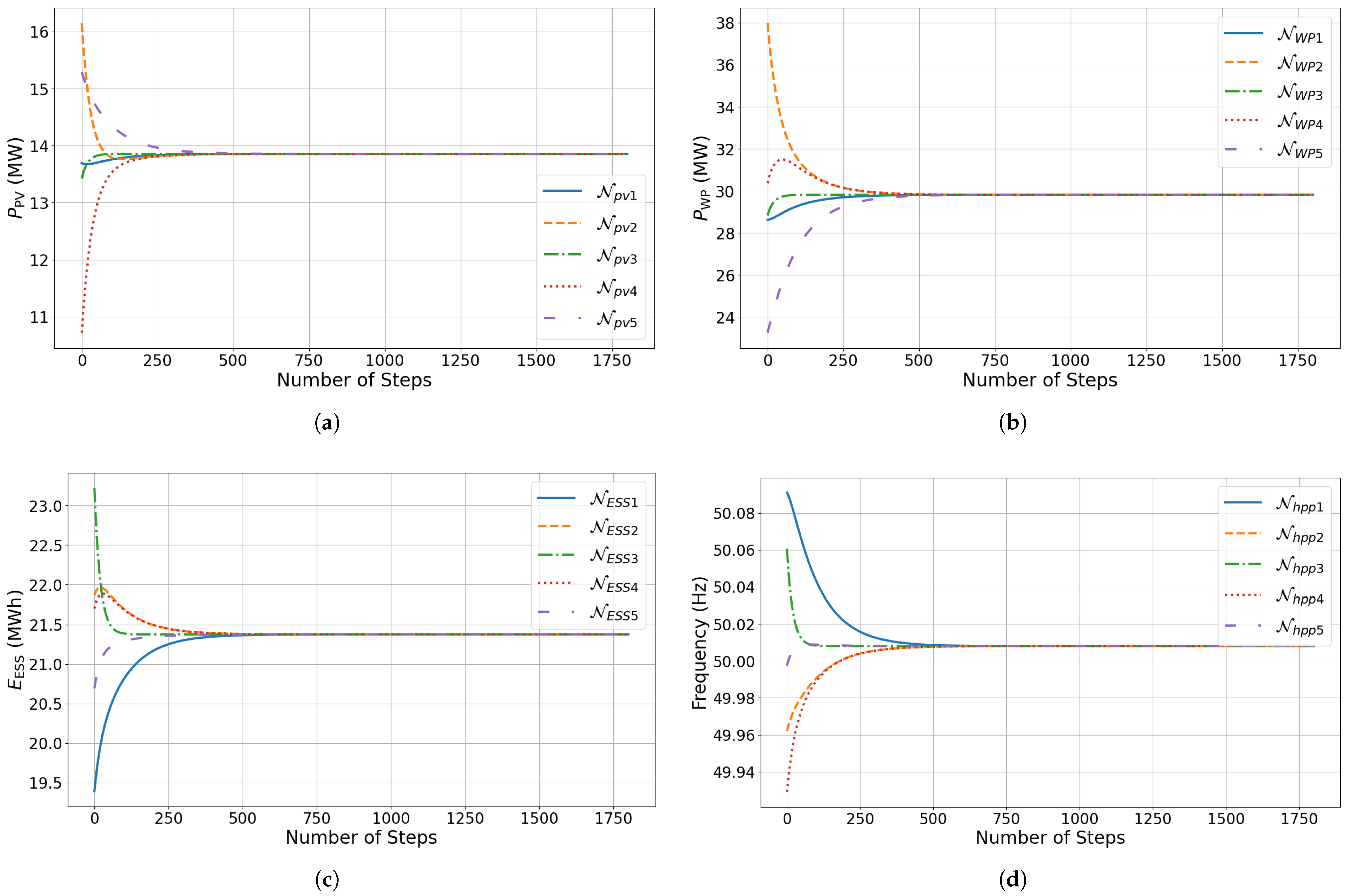
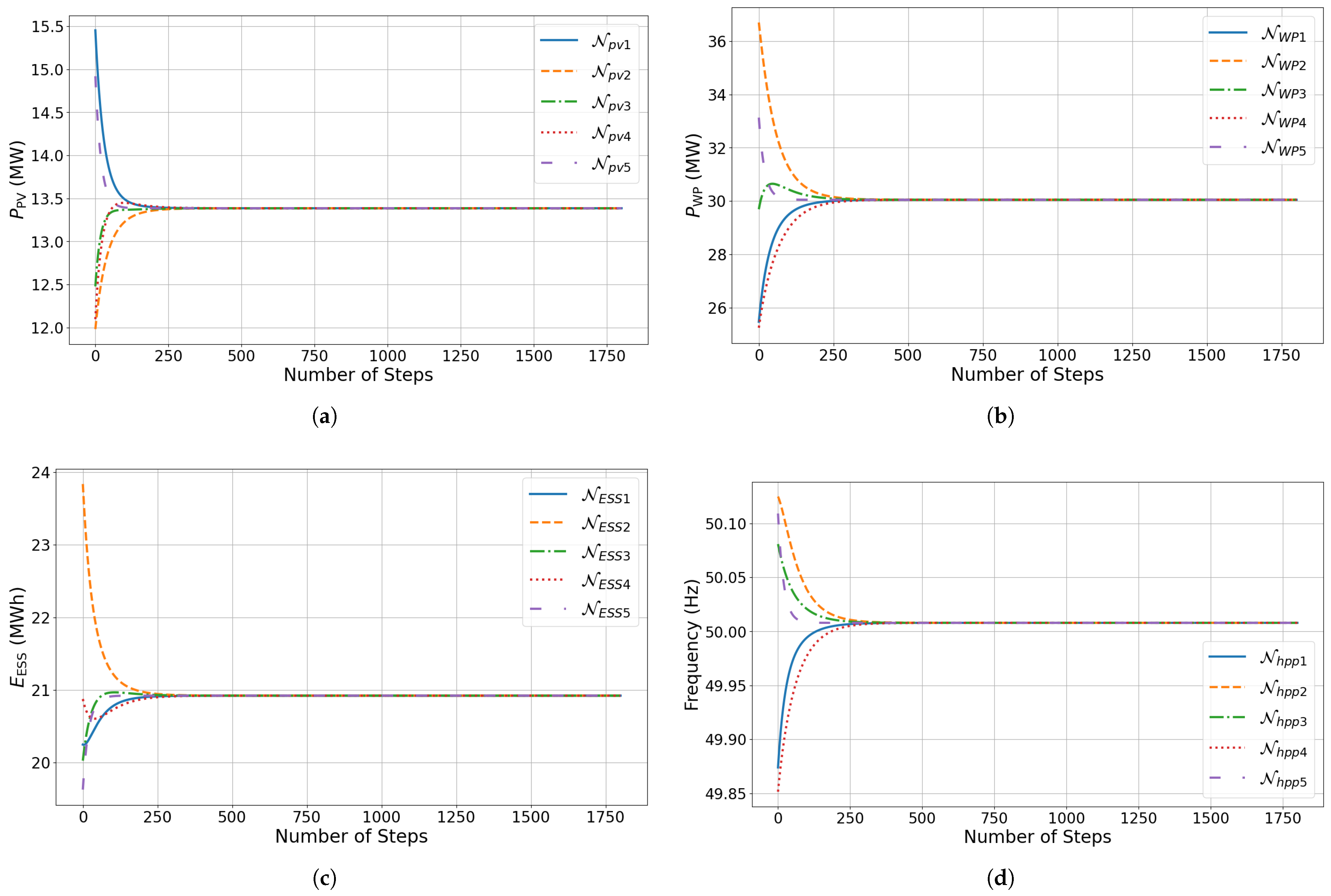
4.3. Optimal Dispatch Analysis

Referring to Equations (22)–(23), the optimal dispatch of the PV, WP, and ESS plants is evaluated considering dynamic, partially-connected, and fully-connected topologies to assess the resiliency of the proposed N—MADRL scheme. This analysis uses the dynamics of the HPP environment from Table 3 and the simulation environment in Figure 6. Figure 9 illustrates the optimal dispatch of HPP assets considering dynamic topologies, as mentioned in Equations (28)–(30).

Referring to Equations (24)–(26), partially-connected and fully-connected communication topologies were considered for optimal dispatch across PV, WP, and ESS zones to observe the influence of communication. Due to the external control inputs of $U_{\mathrm{ij}}^{\mathrm{pv}}$, $U_{\mathrm{ij}}^{\mathrm{wp}}$, and $U_{\mathrm{ij}}^{\mathrm{ess}}$ for policy update $\pi (·\mid {\theta }_{i,j,k}^{\mu })$, the PV, WP, and ESS agents converge rapidly for optimal dispatch after only a few iterations k, as shown in Figure 10 and Figure 11.

5. Discussion and Results Analysis

In this section, the results of the proposed N—MADRL framework are discussed and analysed. We evaluate the robustness of N—MADRL with uncertainty control and communication resiliency to assess the frequency deviation and optimal dispatch objectives. In addition, the results of the performance analysis of the HPP environment and PV, WP, and ESS zones are evaluated and assessed in detail.

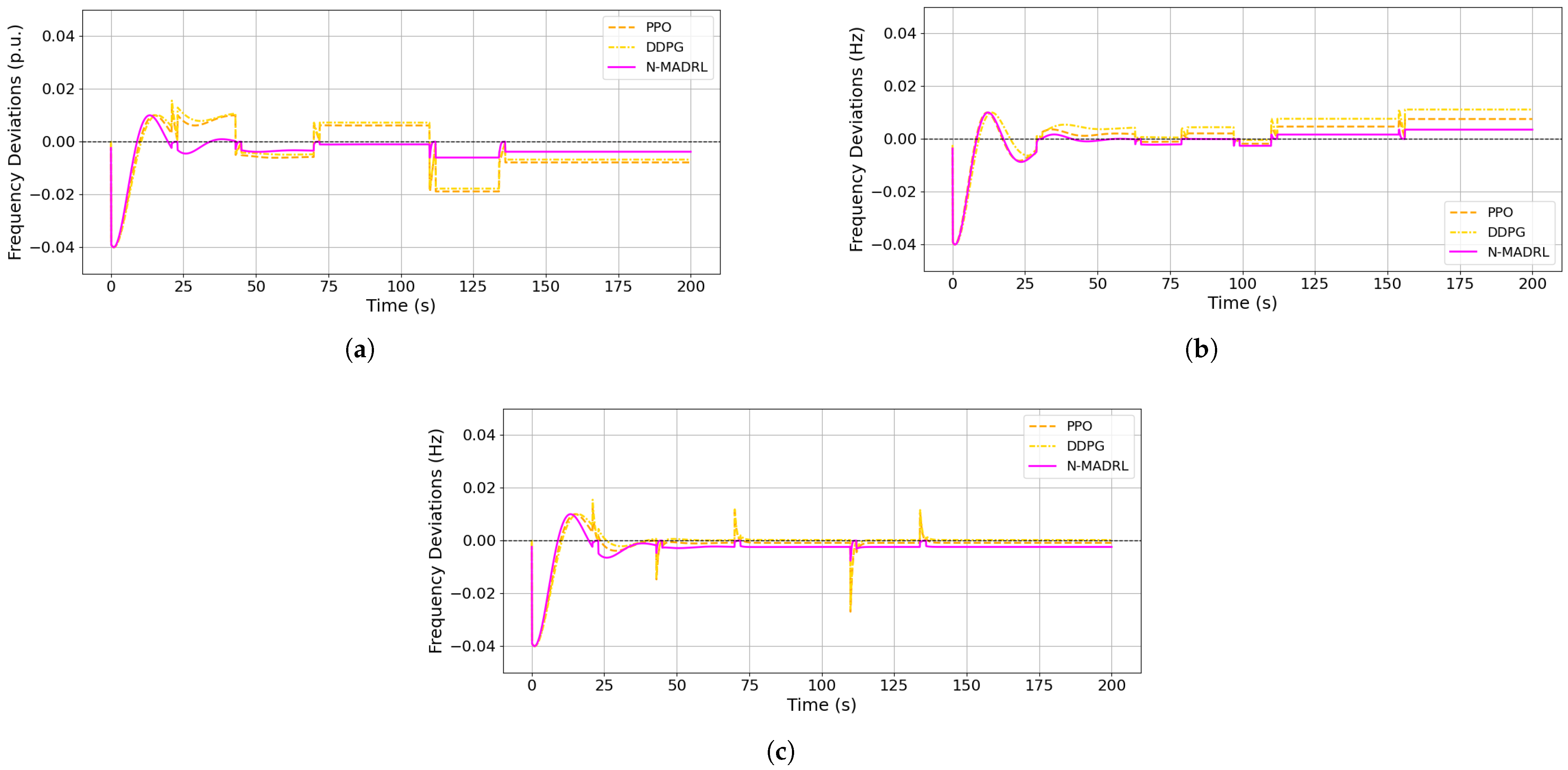
5.1. Robustness Analysis

The robustness of the proposed N—MADRL framework was analysed and evaluated with uncertainty control to assess the training resiliency with random samples. In addition, the communication resiliency was evaluated for partially-connected and fully-connected communication topologies in order to assess the stability of training and learning control policies.

5.1.1. Uncertainty Control

The uncertainty of the HPP environment was considered for PV and WP plants due to their intermittent nature, which is established by different scenarios. Standard deviations were introduced into the training of the PV, WP, and ESS plants, represented with $\{{\sigma }_{\mathrm{PV}},{\sigma }_{\mathrm{WP}},{\sigma }_{\mathrm{ESS}}\}$. As the PV, WP, and ESS assets contribute uniformly for optimal dispatch, we introduced random variation for building uncertainties such as $\{\mathrm{rand}\left({\sigma }_{\mathrm{PV}}\right),\mathrm{rand}\left({\sigma }_{\mathrm{WP}}\right),\mathrm{rand}\left({\sigma }_{\mathrm{ESS}}\right)\}$. In this way, the power generation $P_{\mathrm{PV}}$, $P_{\mathrm{WP}}$, $P_{\mathrm{ESS}}$ and optimal dispatch for $P_{\mathrm{HP}}$ and $f_{\mathrm{HP}}$ will be $\{P_{\mathrm{PV}}+\mathrm{rand}\left({\sigma }_{\mathrm{PV}}\right)\}$, $\{P_{\mathrm{WP}}+\mathrm{rand}\left({\sigma }_{\mathrm{WP}}\right)\}$, and $\{P_{\mathrm{ESS}}+\mathrm{rand}\left({\sigma }_{\mathrm{ESS}}\right)\}$.

Randomly generated training samples were chosen for the proposed N—MADRL model to validate this claim. Figure 12 shows the variations in inertial response, cumulative reward, and frequency deviation under uncertainty situations. The frequency deviation increases as the power generation peaks in the middle of the day. The variations in optimal dispatch of $P_{\mathrm{HP}}$ and frequency $f_{\mathrm{HP}}$ stabilise for N—MADRL due to execution of the optimal policy $\pi (·\mid {\theta }_{i,j,k}^{\mu })$ and maximisation of $\mathcal{H}\left(\pi (·\mid s_k)\right)$ entropy regularisation. In this experiment, the performance of the proposed N—MADRL model is again higher than that of PPO and DDPG. At the same time, the frequency deviations in the uncertainty situations remain within the limits for the HPP environment. In uncertain situations, the reward coefficients are balanced to control power imbalances, reserve management, active power sharing, and frequency deviations. Explicitly tuning the frequency deviation factor ${\beta }_2$ could sharpen frequency stability, but results in over-optimising the proposed model, consequently affecting the generalisability of the HPP environment. In addition, the proposed N—MADRL model considers weighted reward factors ${\beta }_1-{\beta }_4$ that closely associate active power balancing, reserve management, and improving frequency deviations.

5.1.2. Communication Resiliency

Communication resiliency is considered in the HPP environment by changing communication topologies among $P_{\mathrm{PV}}$, $P_{\mathrm{WP}}$, and $P_{\mathrm{ESS}}$ agents. The impact of changing communication topologies ultimately changes $r_{hpp}^t$ due to the updated policy $\pi (·\mid {\theta }_{i,j,k}^{\mu })$. The following scenarios involving changing communication topologies were considered:

• Scenario One (S 1): In this scenario, every agent $P_{\mathrm{PV}}$, $P_{\mathrm{WP}}$, $P_{\mathrm{ESS}}$ is fully connected in each zone during the training process of the DDPG, PPO, and N—MADRL algorithms.
• Scenario Two (S 2): In this scenario, every agent in $P_{\mathrm{PV}}$, $P_{\mathrm{WP}}$, $P_{\mathrm{ESS}}$ is partially connected in their respective zones during the training process for the DDPG, PPO, and N—MADRL algorithms.

The communication topologies were selected by dynamically assigning the convergence rate, such as ${\alpha }^{\mathrm{pv}},{\alpha }^{\mathrm{wp}},{\alpha }^{\mathrm{ess}}$. For fully connected communication topologies, the range was dynamically changing between 0.60 and 0.70, with every agent connected with neighbour agents in mesh topologies. For the partially-connected communication topologies, the rate of convergence of ${\alpha }^{\mathrm{pv}},{\alpha }^{\mathrm{wp}},{\alpha }^{\mathrm{ess}}$ was set to 0.35 to 0.45, with every agent connected with at least one neighbour agent to exchange control inputs $U_{\mathrm{ij}}^{\mathrm{pv}}$, $U_{\mathrm{ij}}^{\mathrm{wp}}$, $U_{\mathrm{ij}}^{\mathrm{ess}}$. For randomly-connected communication topologies, the convergence rate of ${\alpha }^{\mathrm{pv}},{\alpha }^{\mathrm{wp}},{\alpha }^{\mathrm{ess}}$ was set between 0.35 to 0.70, in which the number of connections was changed after every iteration when learning the control policies. Conversely, if the range of fully-connected communication topologies is considered, there are 60% to 70% connections are available to for the exchange of control inputs $U_{\mathrm{ij}}^{\mathrm{pv}}$, $U_{\mathrm{ij}}^{\mathrm{wp}}$, $U_{\mathrm{ij}}^{\mathrm{ess}}$. In addition, if the range of partially-connected communication topologies are considered, there are 35% to 45% connections available for the exchange of control inputs $U_{\mathrm{ij}}^{\mathrm{pv}}$, $U_{\mathrm{ij}}^{\mathrm{wp}}$, $U_{\mathrm{ij}}^{\mathrm{ess}}$. Moreover, the dynamically-connected communication topologies use 35% to 70% connections to share the control input $U_{\mathrm{ij}}^{\mathrm{pv}}$, $U_{\mathrm{ij}}^{\mathrm{wp}}$, $U_{\mathrm{ij}}^{\mathrm{ess}}$ within the HPP environment.

From Figure 13, fully-connected topologies are considered for each zone to observe the performance of DDPG, PPO, and N—MADRL schemes for the frequency stability. The disturbances are randomly initiated for PV, WP, and ESS zones to observe the frequency deviations. The highest-frequency deviations are observed for DDPG, which uses a single-agent replay buffer and contains local state information in the absence of external control inputs of $U_{\mathrm{ij}}^{\mathrm{pv}}$, $U_{\mathrm{ij}}^{\mathrm{wp}}$, $U_{\mathrm{ij}}^{\mathrm{ess}}$. Similarly, the PPO algorithm is an interacting environment for the policy update $\pi (·\mid {\theta }_{i,j,k}^{\mu })$, and is executed locally without considering the dynamics of the HPP environment. Our proposed N—MADRL provides robust performance due to its full coordination and control among HPP agents.

Referring to Figure 14, a partially-connected communication topology is considered and a disturbance is initiated at times $t=22$ s, $t=16$ s, and $t=12$ s to observe the frequency deviations in the PV, WP, and ESS zones. Initially, the results of the DDPG scheme show higher fluctuations and damping due to the overestimation of Q-values and insufficient coordination among HPP agents. In contrast, the performance of the PPO algorithm is satisfactory compared to DDPG due to its stochastic policy and stable training. The proposed N—MADRL model achieves the highest performance due to its independent training, shared reward maximisation, and ability to handle nonstationary behaviour on the part of HPP agents. Based on these results, N—MADRL provides optimal performance compared to DDPG and PPO in both scenarios.

The purpose of considering both partially- and fully-connected communication topologies is for a realistic communication approximation of delay-dependent systems. The quantification of delay attributes and latency models is not investigated for the N—MADRL approach. The proposed N—MADRL approach maintains optimal performance in both communication scenarios without affecting the learning policies or robustness.

Table 6. Control performance of DRL algorithms under partially-connected and full-connected communication topologies.

Scenarios	Algorithms	Rewards	Deviation (Hz)	Std. Deviation	Convergence Rate	Threshold	Steps
Scenario 1	N—MADRL	−25	0.085	4.37	0.61	61%	21,100
	PPO	−54	0.098	7.11	0.64	64%	28,400
	DDPG	−128	0.106	9.34	0.62	62%	–
Scenario 2	N—MADRL	−35	0.092	4.37	0.37	37%	33,200
	PPO	−70	0.103	6.48	0.41	41%	41,230
	DDPG	−135	0.160	7.15	0.39	39%	–

illustrates the control performance of the proposed algorithm in terms of optimal dispatch, minimised frequency deviation, and communication resiliency.

5.2. Performance Analysis

The results of the N—MADRL approach were experimented on using the Grid2Op power simulation environment of the IEEE 14 bus network with the participation of PV, WP, and ESS plants. The random communication scenario was considered, referring to Equations (24)–(30) to check the overall performance of communication influence. In the random topology, the control inputs of the PV, WP, and ESS agents $U_{\mathrm{ij}}^{\mathrm{pv}}$, $U_{\mathrm{ij}}^{\mathrm{wp}}$, and $U_{\mathrm{ij}}^{\mathrm{ess}}$ are coordinated with neighbour agents for estimation of the global status $P_{\mathrm{PV}}(k+1)$, $P_{\mathrm{WP}}(k+1)$, and $P_{\mathrm{ESS}}(k+1)$ respectively.

The factors ${\alpha }^{\mathrm{pv}},{\alpha }^{\mathrm{wp}},{\alpha }^{\mathrm{ess}}$ decide the speed of convergence and coordination for the frequency control, as shown in Figure 9. Referring to Equation (27), the optimal range of ${\alpha }^{\mathrm{pv}},{\alpha }^{\mathrm{wp}},{\alpha }^{\mathrm{ess}}$ is between 0.550 and 0.710 for connected topologies. For the dynamic topology, the control policy $\pi (·\mid {\theta }_{i,j,k}^{\mu })$ changes for the $P_{\mathrm{PV}}\left(k\right)$, $P_{\mathrm{WP}}\left(k\right)$, $P_{\mathrm{ESS}}\left(k\right)$ plants. Due to the adaptive nature and communication resiliency of the proposed N—MADRL approach, the cumulative rewards and frequency deviation control outperform those of DDPG and PPO algorithms, as shown in Figure 15.

Referring to Table 3, the performance of the PV, WP, and ESS zones is analysed along with its impact on the HPP environment for the optimal dispatch and control of frequency deviations.

Table 7. Performance of the PV plant in IEEE 14 bus systems.

g-id	Bus	${\mathit{\alpha }}^{\mathbf{pv}}$	${\mathit{U}}_{\mathbf{ij}}^{\mathbf{pv}}$	${\mathit{P}}_{\mathbf{PV}}^{\mathit{c}}$	${\mathit{R}}_{\mathbf{PV}}$
0	1	0.618	0.039	11.7	2.34
4	2	0.562	0.036	14.8	2.96
6	4	0.647	0.034	17.6	3.52
9	11	0.683	0.037	10.4	2.08
12	8	0.594	0.035	10.7	2.14
13	14	0.616	0.038	12.2	2.44

represents the control performance of the PV plant, which is examined under the dynamic communication topology for the control of frequency deviations. Due to the optimal reserve margin $R_{\mathrm{PV}}$ and convergence ${\alpha }^{\mathbf{pv}}$ factors, the frequency deviations for N—MADRL exhibit the lowest susceptibility as compared to PPO and DDPG, as shown in Figure 16a.

Similarly, the control performance of the WP plant was observed for the control of frequency deviations under the time-varying communication topologies, as shown in

Table 8. Performance of the WP plant in IEEE 14 bus systems.

g-id	Bus	${\mathit{\alpha }}^{\mathbf{wp}}$	${\mathit{U}}_{\mathbf{ij}}^{\mathbf{wp}}$	${\mathit{P}}_{\mathbf{WP}}^{\mathit{c}}$	${\mathit{R}}_{\mathbf{WP}}$
2	3	0.594	0.026	26.7	5.34
5	6	0.631	0.023	41.4	8.28
8	9	0.658	0.025	33.4	6.68
10	7	0.614	0.021	22.8	4.56

. Due to the optimal control inputs ${\mathit{U}}_{\mathbf{ij}}^{\mathbf{wp}}$ and converging factor ${\alpha }^{\mathbf{wp}}$, the control performance of the WP zone provides more stability for the N—MADRL approach as compared to PPO and DDPG, as shown in Figure 16b.

In addition, the control of frequency deviations in the ESS plant exhibits similar results under the random communication topologies, as shown in Figure 16c.

Table 9. Performance of the ESS plant in IEEE 14 bus systems.

g-id	Bus	${\mathit{\alpha }}^{\mathbf{ess}}$	${\mathit{U}}_{\mathbf{ij}}^{\mathbf{ess}}$	${\mathit{P}}_{\mathbf{ESS}}^{\mathit{c}}$	${\mathit{R}}_{\mathbf{ESS}}$
1	5	0.670	0.032	21.8	4.36
3	12	0.621	0.030	25.75	5.15
7	13	0.632	0.029	18.6	3.72
11	10	0.594	0.031	22.7	4.54

refers to the control inputs ${\mathit{U}}_{\mathbf{ij}}^{\mathbf{ess}}$, ${\alpha }^{\mathbf{ess}}$, ${\mathit{R}}_{\mathbf{ESS}}$, with the performance of the N—MADRL approach in the ESS zone demonstrating lower susceptibility to frequency deviations compared to the PPO and DDPG schemes.

Due to the heterogeneity and optimal coordination of the N—MADRL model, Figure 16 exhibits an adaptive and flexible approach for the HPP environment to provide fast-changing control inputs $U_{\mathrm{ij},\mathrm{t}}^{\mathrm{pv}}$, $U_{\mathrm{ij},\mathrm{t}}^{\mathrm{wp}}$, $U_{\mathrm{ij},\mathrm{t}}^{\mathrm{ess}}$, converging factors ${\alpha }^{\mathrm{pv}},{\alpha }^{\mathrm{wp}},{\alpha }^{\mathrm{ess}}$, and reserve margins $R_{\mathrm{PV}}$, $R_{\mathrm{WP}}$, $R_{\mathrm{ESS}}$ for the stability of frequency and optimal dispatch. Moreover, Table 7, Table 8 and Table 9 provide more insights into different scenarios of HPP zones for the stability of frequency control and performance improvement of the HPP environment under dynamic communication topologies. The individual assets of the PV, WP, and ESS plants are considered for frequency control using physical constraints, and the communication resiliency is assessed with numerous topologies and control inputs.

6. Conclusions

This paper presents the novel N—MADRL actor-critic architecture by developing a model-free environment to coordinate PV, WP, and ESS plants in the HPP environment. The proposed N—MADRL approach aims to maintain frequency stability by optimal dispatch of active power, thereby mitigating frequency deviations, optimising reserve management, and improving power sharing capabilities. The results indicate that 1 compared to the PPO and DDPG schemes, the proposed N—MADRL approach achieves 42.10% and 61.40% higher efficiency for optimal dispatch and 68.30% and 74.48% improvement in mitigation of frequency deviations, respectively; 2 due to the intermittent nature of PV and WP plants, the results for various control scenarios examined to assess the performance of the proposed approach indicate that its optimal dispatch and reserve management effectively minimise frequency deviations; 3 considering random, partial, and fully-connected communication topologies for the PV, WP, and ESS plants assessed at different timescales, our proposed scheme exhibits robust performance and higher communication resiliency than the PPO and DDPG schemes, demonstrating robustness to communication vulnerabilities in the HPP environment; 4 the dynamic performance and scalability of the HPP environment were evaluated for optimal power dispatch and energy reserve management to reduce frequency deviations, with the results indicating that N—MADRL demonstrates the lowest susceptibility to frequency deviations compared to the PPO and DDPG approaches. The proposed framework addresses optimal dispatch problems using a decentralised coordination mechanism to enhance the operational stability and frequency security of the HPP environment. Physical constraints such as active power sharing, energy reserve margins, and frequency deviations are considered when updating the policy network. The proposed N—MADRL agents rely solely on local control parameters within each HPP zone for frequency control and stability. Furthermore, a dynamic Grid2Op simulation environment was considered, with the results demonstrated on the IEEE 14 bus network to validate the effectiveness of the N—MADRL approach in handling uncertainty, system intermittency, and communication resiliency. The proposed N—MADRL approach is ready to deploy for transmission system operators for optimal dispatch and frequency control. It can provide grid support services in steady-state and emergency control by responding to power imbalances and system disturbances. In future work, this research could be extended to the provision of fast frequency control ancillary services by considering the influence of inverter dynamics, ESS cost-oriented rewards formulation, the control parameters, and the optimisation of frequency response. The electric power industry must enable fast frequency support ancillary services from IBR-enabled HPP to meet inertial requirements and rapid frequency regulations in modern power grids.

References

1. Čović, N.; Pavić, I.; Pandžić, H. Multi-energy balancing services provision from a hybrid power plant: PV, battery, and hydrogen technologies. Appl. Energy 2024, 374, 123966. [Google Scholar] [CrossRef]
2. Klyve, Ø.S.; Grab, R.; Olkkonen, V.; Marstein, E.S. Influence of high-resolution data on accurate curtailment loss estimation and optimal design of hybrid PV–wind power plants. Appl. Energy 2024, 372, 123784. [Google Scholar] [CrossRef]
3. Kim, Y.S.; Park, G.H.; Kim, S.W.; Kim, D. Incentive design for hybrid energy storage system investment to PV owners considering value of grid services. Appl. Energy 2024, 373, 123772. [Google Scholar] [CrossRef]
4. Zhang, T.; Xin, L.; Wang, S.; Guo, R.; Wang, W.; Cui, J.; Wang, P. A novel approach of energy and reserve scheduling for hybrid power systems: Frequency security constraints. Appl. Energy 2024, 361, 122926. [Google Scholar] [CrossRef]
5. Askarov, A.; Rudnik, V.; Ruban, N.; Radko, P.; Ilyushin, P.; Suvorov, A. Enhanced Virtual Synchronous Generator with Angular Frequency Deviation Feedforward and Energy Recovery Control for Energy Storage System. Mathematics 2024, 12, 2691. [Google Scholar] [CrossRef]
6. Leng, D.; Polmai, S. Virtual Synchronous Generator Based on Hybrid Energy Storage System for PV Power Fluctuation Mitigation. Appl. Sci. 2019, 9, 5099. [Google Scholar] [CrossRef]
7. Pourbeik, P.; Sanchez-Gasca, J.J.; Senthil, J.; Weber, J.; Zadkhast, P.; Ramasubramanian, D.; Rao, S.D.; Bloemink, J.; Majumder, R.; Zhu, S.; et al. A Generic Model for Inertia-Based Fast Frequency Response of Wind Turbines and Other Positive-Sequence Dynamic Models for Renewable Energy Systems. IEEE Trans. Energy Convers. 2024, 39, 425–434. [Google Scholar] [CrossRef]
8. Long, Q.; Das, K.; Pombo, D.V.; Sørensen, P.E. Hierarchical control architecture of co-located hybrid power plants. Int. J. Electr. Power Energy Syst. 2022, 143, 108407. [Google Scholar] [CrossRef]
9. Ekomwenrenren, E.; Simpson-Porco, J.W.; Farantatos, E.; Patel, M.; Haddadi, A.; Zhu, L. Data-Driven Fast Frequency Control Using Inverter-Based Resources. IEEE Trans. Power Syst. 2024, 39, 5755–5768. [Google Scholar] [CrossRef]
10. Jendoubi, I.; Bouffard, F. Multi-agent hierarchical reinforcement learning for energy management. Appl. Energy 2023, 332, 120500. [Google Scholar] [CrossRef]
11. Guruwacharya, N.; Chakraborty, S.; Saraswat, G.; Bryce, R.; Hansen, T.M.; Tonkoski, R. Data-Driven Modeling of Grid-Forming Inverter Dynamics Using Power Hardware-in-the-Loop Experimentation. IEEE Access 2024, 12, 52267–52281. [Google Scholar] [CrossRef]
12. Zhu, D.; Yang, B.; Liu, Y.; Wang, Z.; Ma, K.; Guan, X. Energy management based on multi-agent deep reinforcement learning for a multi-energy industrial park. Appl. Energy 2022, 311, 118636. [Google Scholar] [CrossRef]
13. Li, Y.; Hou, J.; Yan, G. Exploration-enhanced multi-agent reinforcement learning for distributed PV-ESS scheduling with incomplete data. Appl. Energy 2024, 359, 122744. [Google Scholar] [CrossRef]
14. Ochoa, T.; Gil, E.; Angulo, A.; Valle, C. Multi-agent deep reinforcement learning for efficient multi-timescale bidding of a hybrid power plant in day-ahead and real-time markets. Appl. Energy 2022, 317, 119067. [Google Scholar] [CrossRef]
15. Jin, R.; Zhou, Y.; Lu, C.; Song, J. Deep reinforcement learning-based strategy for charging station participating in demand response. Appl. Energy 2022, 328, 120140. [Google Scholar] [CrossRef]
16. Vázquez-Canteli, J.R.; Nagy, Z. Reinforcement learning for demand response: A review of algorithms and modeling techniques. Appl. Energy 2019, 235, 1072–1089. [Google Scholar] [CrossRef]
17. Xia, Q.; Wang, Y.; Zou, Y.; Yan, Z.; Zhou, N.; Chi, Y.; Wang, Q. Regional-privacy-preserving operation of networked microgrids: Edge-cloud cooperative learning with differentiated policies. Appl. Energy 2024, 370, 123611. [Google Scholar] [CrossRef]
18. Sun, X.; Xie, H.; Qiu, D.; Xiao, Y.; Bie, Z.; Strbac, G. Decentralized frequency regulation service provision for virtual power plants: A best response potential game approach. Appl. Energy 2023, 352, 121987. [Google Scholar] [CrossRef]
19. Kofinas, P.; Dounis, A.I.; Vouros, G.A. Fuzzy Q-Learning for multi-agent decentralized energy management in microgrids. Appl. Energy 2018, 219, 53–67. [Google Scholar] [CrossRef]
20. May, R.; Huang, P. A multi-agent reinforcement learning approach for investigating and optimising peer-to-peer prosumer energy markets. Appl. Energy 2023, 334, 120705. [Google Scholar] [CrossRef]
21. Zhang, B.; Hu, W.; Ghias, A.M.; Xu, X.; Chen, Z. Two-timescale autonomous energy management strategy based on multi-agent deep reinforcement learning approach for residential multicarrier energy system. Appl. Energy 2023, 351, 121777. [Google Scholar] [CrossRef]
22. Xu, X.; Xu, K.; Zeng, Z.; Tang, J.; He, Y.; Shi, G.; Zhang, T. Collaborative optimization of multi-energy multi-microgrid system: A hierarchical trust-region multi-agent reinforcement learning approach. Appl. Energy 2024, 375, 123923. [Google Scholar] [CrossRef]
23. Lv, C.; Liang, R.; Zhang, G.; Zhang, X.; Jin, W. Energy accommodation-oriented interaction of active distribution network and central energy station considering soft open points. Energy 2023, 268, 126574. [Google Scholar] [CrossRef]
24. Wang, Y.; Cui, Y.; Li, Y.; Xu, Y. Collaborative optimization of multi-microgrids system with shared energy storage based on multi-agent stochastic game and reinforcement learning. Energy 2023, 280, 128182. [Google Scholar] [CrossRef]
25. Bui, V.H.; Su, W. Real-time operation of distribution network: A deep reinforcement learning-based reconfiguration approach. Sustain. Energy Technol. Assess. 2022, 50, 101841. [Google Scholar] [CrossRef]
26. Li, H.; He, H. Optimal Operation of Networked Microgrids With Distributed Multi-Agent Reinforcement Learning. In Proceedings of the 2024 IEEE Power & Energy Society General Meeting (PESGM), Seattle, WA, USA, 21–25 July 2024; pp. 1–5. [Google Scholar]
27. Fang, X.; Wang, J.; Song, G.; Han, Y.; Zhao, Q.; Cao, Z. Multi-agent reinforcement learning approach for residential microgrid energy scheduling. Energies 2019, 13, 123. [Google Scholar] [CrossRef]
28. Anjaiah, K.; Dash, P.; Bisoi, R.; Dhar, S.; Mishra, S. A new approach for active and reactive power management in renewable based hybrid microgrid considering storage devices. Appl. Energy 2024, 367, 123429. [Google Scholar] [CrossRef]
29. Wu, H.; Qiu, D.; Zhang, L.; Sun, M. Adaptive multi-agent reinforcement learning for flexible resource management in a virtual power plant with dynamic participating multi-energy buildings. Appl. Energy 2024, 374, 123998. [Google Scholar] [CrossRef]
30. Zhao, H.; Wang, B.; Liu, H.; Sun, H.; Pan, Z.; Guo, Q. Exploiting the flexibility inside park-level commercial buildings considering heat transfer time delay: A memory-augmented deep reinforcement learning approach. IEEE Trans. Sustain. Energy 2021, 13, 207–219. [Google Scholar] [CrossRef]
31. Ebrie, A.S.; Kim, Y.J. Reinforcement Learning-Based Multi-Objective Optimization for Generation Scheduling in Power Systems. Systems 2024, 12, 106. [Google Scholar] [CrossRef]
32. Qiu, D.; Wang, Y.; Zhang, T.; Sun, M.; Strbac, G. Hybrid Multiagent Reinforcement Learning for Electric Vehicle Resilience Control Towards a Low-Carbon Transition. IEEE Trans. Ind. Inform. 2022, 18, 8258–8269. [Google Scholar] [CrossRef]
33. Wang, Y.; Qiu, D.; Strbac, G.; Gao, Z. Coordinated Electric Vehicle Active and Reactive Power Control for Active Distribution Networks. IEEE Trans. Ind. Inform. 2023, 19, 1611–1622. [Google Scholar] [CrossRef]
34. Singh, V.P.; Kishor, N.; Samuel, P. Distributed Multi-Agent System-Based Load Frequency Control for Multi-Area Power System in Smart Grid. IEEE Trans. Ind. Electron. 2017, 64, 5151–5160. [Google Scholar] [CrossRef]
35. Yu, T.; Wang, H.Z.; Zhou, B.; Chan, K.W.; Tang, J. Multi-Agent Correlated Equilibrium Q(λ) Learning for Coordinated Smart Generation Control of Interconnected Power Grids. IEEE Trans. Power Syst. 2015, 30, 1669–1679. [Google Scholar] [CrossRef]
36. Shen, R.; Zhong, S.; Wen, X.; An, Q.; Zheng, R.; Li, Y.; Zhao, J. Multi-agent deep reinforcement learning optimization framework for building energy system with renewable energy. Appl. Energy 2022, 312, 118724. [Google Scholar] [CrossRef]
37. Lu, R.; Li, Y.C.; Li, Y.; Jiang, J.; Ding, Y. Multi-agent deep reinforcement learning based demand response for discrete manufacturing systems energy management. Appl. Energy 2020, 276, 115473. [Google Scholar] [CrossRef]
38. Wu, J.; He, H.; Peng, J.; Li, Y.; Li, Z. Continuous reinforcement learning of energy management with deep Q network for a power split hybrid electric bus. Appl. Energy 2018, 222, 799–811. [Google Scholar] [CrossRef]
39. Ajagekar, A.; Decardi-Nelson, B.; You, F. Energy management for demand response in networked greenhouses with multi-agent deep reinforcement learning. Appl. Energy 2024, 355, 122349. [Google Scholar] [CrossRef]
40. Wang, Y.; Qiu, D.; Strbac, G. Multi-agent deep reinforcement learning for resilience-driven routing and scheduling of mobile energy storage systems. Appl. Energy 2022, 310, 118575. [Google Scholar] [CrossRef]
41. Zhang, J.; Sang, L.; Xu, Y.; Sun, H. Networked Multiagent-Based Safe Reinforcement Learning for Low-Carbon Demand Management in Distribution Networks. IEEE Trans. Sustain. Energy 2024, 15, 1528–1545. [Google Scholar] [CrossRef]
42. Tavakol Aghaei, V.; Ağababaoğlu, A.; Bawo, B.; Naseradinmousavi, P.; Yıldırım, S.; Yeşilyurt, S.; Onat, A. Energy optimization of wind turbines via a neural control policy based on reinforcement learning Markov chain Monte Carlo algorithm. Appl. Energy 2023, 341, 121108. [Google Scholar] [CrossRef]
43. Li, J.; Yu, T.; Zhang, X. Coordinated load frequency control of multi-area integrated energy system using multi-agent deep reinforcement learning. Appl. Energy 2022, 306, 117900. [Google Scholar] [CrossRef]
44. Dong, L.; Lin, H.; Qiao, J.; Zhang, T.; Zhang, S.; Pu, T. A coordinated active and reactive power optimization approach for multi-microgrids connected to distribution networks with multi-actor-attention-critic deep reinforcement learning. Appl. Energy 2024, 373, 123870. [Google Scholar] [CrossRef]
45. Deptula, P.; Bell, Z.I.; Doucette, E.A.; Curtis, J.W.; Dixon, W.E. Data-based reinforcement learning approximate optimal control for an uncertain nonlinear system with control effectiveness faults. Automatica 2020, 116, 108922. [Google Scholar] [CrossRef]
46. Zhang, B.; Cao, D.; Hu, W.; Ghias, A.M.; Chen, Z. Physics-Informed Multi-Agent deep reinforcement learning enabled distributed voltage control for active distribution network using PV inverters. Int. J. Electr. Power Energy Syst. 2024, 155, 109641. [Google Scholar] [CrossRef]
47. Li, S.; Hu, W.; Cao, D.; Chen, Z.; Huang, Q.; Blaabjerg, F.; Liao, K. Physics-model-free heat-electricity energy management of multiple microgrids based on surrogate model-enabled multi-agent deep reinforcement learning. Appl. Energy 2023, 346, 121359. [Google Scholar] [CrossRef]
48. Abid, M.S.; Apon, H.J.; Hossain, S.; Ahmed, A.; Ahshan, R.; Lipu, M.H. A novel multi-objective optimization based multi-agent deep reinforcement learning approach for microgrid resources planning. Appl. Energy 2024, 353, 122029. [Google Scholar] [CrossRef]
49. Hua, M.; Zhang, C.; Zhang, F.; Li, Z.; Yu, X.; Xu, H.; Zhou, Q. Energy management of multi-mode plug-in hybrid electric vehicle using multi-agent deep reinforcement learning. Appl. Energy 2023, 348, 121526. [Google Scholar] [CrossRef]
50. Xie, J.; Ajagekar, A.; You, F. Multi-Agent attention-based deep reinforcement learning for demand response in grid-responsive buildings. Appl. Energy 2023, 342, 121162. [Google Scholar] [CrossRef]
51. Xiang, Y.; Lu, Y.; Liu, J. Deep reinforcement learning based topology-aware voltage regulation of distribution networks with distributed energy storage. Appl. Energy 2023, 332, 120510. [Google Scholar] [CrossRef]
52. Guo, G.; Zhang, M.; Gong, Y.; Xu, Q. Safe multi-agent deep reinforcement learning for real-time decentralized control of inverter based renewable energy resources considering communication delay. Appl. Energy 2023, 349, 121648. [Google Scholar] [CrossRef]
53. Si, R.; Chen, S.; Zhang, J.; Xu, J.; Zhang, L. A multi-agent reinforcement learning method for distribution system restoration considering dynamic network reconfiguration. Appl. Energy 2024, 372, 123625. [Google Scholar] [CrossRef]
54. Tzani, D.; Stavrakas, V.; Santini, M.; Thomas, S.; Rosenow, J.; Flamos, A. Pioneering a performance-based future for energy efficiency: Lessons learnt from a comparative review analysis of pay-for-performance programmes. Renew. Sustain. Energy Rev. 2022, 158, 112162. [Google Scholar] [CrossRef]
55. Donnot, B. *Grid2Op: A Testbed Platform to Model Sequential Decision Making in Power Systems*. Available online: https://github.com/Grid2op/grid2op (accessed on 31 March 2025).
Figure 1. Illustration of coordination control of a hybrid power plant. The solid line flow denotes bidirectional cyber-physical communication. The dotted lines show the PV, WP, and ESS asset exchange variables at different control levels.
Energies 18 02666 g001
Figure 2. Illustration of heterogeneous HPP agents in the N—MADRL framework. Global state information is used for centralised training and local state information is used for decentralised execution by the PV, WP, and ESS agents.
Energies 18 02666 g002
Figure 3. Illustration of the proposed N—MADRL framework. The samples of HPP agents are trained in the current value network and estimate the Q-value function. The target value network is used as feedback to improve the training stability and sample efficiency.
Energies 18 02666 g003
Figure 4. Flowchart of the proposed N—MADRL framework for optimal dispatch and frequency control observing training stability and model efficiency.
Energies 18 02666 g004
Figure 5. Flowchart of numerical simulations of the proposed N—MADRL framework for optimal dispatch and frequency control.
Energies 18 02666 g005
Figure 6. Grid2Op HPP environment of IEEE 14−bus system for PV, WP, and ESS plants.
Energies 18 02666 g006
Figure 7. Training results in the HPP environment: (a) cumulative rewards of the PPO, DDPG, and N—MADRL algorithms and (b) frequency deviation of the PPO, DDPG, and N—MADRL algorithms.
Energies 18 02666 g007
Figure 8. Frequency deviations in the HPP environment: (a) frequency deviation in the PV zone using the PPO, DDPG, and N—MADRL algorithms; (b) frequency deviation in the WP zone using the PPO, DDPG, and N—MADRL algorithms; (c) frequency deviation in the ESS zone using the PPO, DDPG, and N—MADRL algorithms.
Energies 18 02666 g008
Figure 9. Optimal dispatch under dynamic communications: (a) optimal dispatch PV agents; (b) optimal dispatch WP agents; (c) optimal dispatch of ESS agents; (d) frequency regulation of HPP environment.
Energies 18 02666 g009aEnergies 18 02666 g009b
Figure 10. Optimal dispatch under partial communication: (a) optimal dispatch of P PV agents for f HP ; (b) optimal dispatch of P WP agents for f HP ; (c) optimal dispatch of P ESS agents for f HP ; (d) frequency regulation of HPP f HP by optimal dispatch of P PV , P WP , P ESS agents.
Energies 18 02666 g010
Figure 11. Optimal dispatch under full communication: (a) optimal dispatch of P PV agents for f HP ; (b) optimal dispatch of P WP agents for f HP ; (c) optimal dispatch of P ESS agents for f HP ; (d) frequency regulation of HPP f HP by optimal dispatch of P PV , P WP , P ESS agents.
Energies 18 02666 g011
Figure 12. Uncertainty control in the HPP environment: (a) inertial response of the HPP environment using the PPO, DDPG, and N—MADRL algorithms; (b) cumulative rewards of the HPP environment under uncertainty situations; (c) frequency deviation in the HPP environment under uncertainty situations.
Energies 18 02666 g012
Figure 13. Fully-connected communication topologies: (a) frequency deviations in the PV zone, (b) frequency deviations in the WP zone, and (c) frequency deviations in the ESS zone.
Energies 18 02666 g013
Figure 14. Partially-connected communication topologies: (a) frequency deviations in the PV zone, (b) frequency deviations in the WP zone, and (c) frequency deviations in the ESS zone.
Energies 18 02666 g014
Figure 15. Performance analysis of the HPP environment: (a) cumulative rewards under dynamic communication and (b) frequency deviations under dynamic communication.
Energies 18 02666 g015
Figure 16. Performance analysis of IEEE 14 bus HPP environment: (a) frequency deviation under dynamic communication in the PV zone, (b) frequency deviation under dynamic communication in the WP zone, and (c) frequency deviation under dynamic communication in the ESS zone.
Energies 18 02666 g016