Renewable Electricity Management Cloud System for Smart Communities Using Advanced Machine Learning

Abstract

Based on the renewable energy assessment in 2023, it was found that only 21% of total electricity is generated using renewable sources. As the global demand for electricity rises in the AI world, the need for electricity management will increase and must be optimized. Based on research, many companies are working on green AI electricity management, but few companies are working on predicting shortages. To identify the rising electricity demand, predict the shortage, and to bring attention to consumption, this study focuses on the optimization of solar electricity generation, tracking its consumption, and forecasting the electricity shortages well in advance. This system demonstrates a novel approach using advanced machine learning, deep learning, and reinforcement learning to maximize solar energy utilization. This paper proposes and develops a community-based model that manages and analyzes multiple buildings’ energy usage, allowing the model to perform both distributed and aggregated decision-making, achieving an accuracy of 98.2% using stacking results of models with reinforcement learning. Concerning the real-world problem, this paper provides a sustainable solution by combining data-driven models with reinforcement learning, contributing to the current market need.

1. Introduction

According to a PRNewswire report, the green energy market is expected to expand at an 8.9% compound annual growth rate (CAGR) between 2023 and 2032, from USD 1 trillion in 2022 to USD 2.4 trillion by 2032 [1]. Based on the current US market in 2023, there is 4000 terawatt/hours of electricity demand, and the numbers are only expected to increase. This increasing demand for electricity calls for an advanced management system of green AI services. Despite recent advancements, solar and wind energy are still sporadic and unpredictable, making it difficult to balance supply and demand and store energy. Traditional energy management systems have a propensity to employ rule-based strategies or static heuristics that are unable to adjust to dynamic and actual energy swings. This inadequate forecasting causes blackouts, ineffective energy trading, and resource waste in local communities. Thus, developing a system that manages green energy resources for electricity presents challenges like data storage, data collection, robust model development, and selecting appropriate parameters. To address these challenges, this paper focuses on solar energy, which contributes to 27% of the total generation of renewable resources. Using collected solar data, this paper develops models to predict the short-term electricity generation, consumption, and shortage.

Data from three different sources at intervals of 30 min for 3 years were collected and stored on the AWS cloud. The designed system uses various machine learning, deep learning, and reinforcement learning methods to design models that are robust in analyzing demand. Using existing methods, this research proposes a model called the Community-Based Model which has been developed through a combination of aggregated and distributed training. The important parameters for developing this model are weather parameters (temperature, humidity, snow, dew, sea level pressure, cloud cover, visibility, precipitation index), solar parameters (solar radiation, beam irradiance, diffuse irradiance, reflected irradiance, and historical solar data), and seasonal parameters (date and time). The system also takes into consideration the concept of the duck curve, which graphically represents electricity demand from the grid on days when solar energy production is high and demand is low. This curve illustrates the challenge of balancing electricity supply and demand when renewable energy sources like solar, which are intermittent and weather-dependent, have a significant impact on energy consumption [2].

To showcase the models’ results, a data-driven decision-making system was designed to analyze and monitor electricity trends, patterns, and demands. To support the Renewable Electricity Management Cloud System for shortage forecasting, this research uses a robust database to store input data and results generated by various models. This research focuses on the short-term to mid-term forecasting, and analyzes data at three different time intervals: hourly, daily, and weekly.

The system can be seamlessly integrated with any energy provider and expanded to mobile applications, providing users with dependable real-time forecasts and the ability to automate procedures related to shortage detection. In addition, the system is lightweight and portable, requiring less than 1 GB of source code, which makes it perfect for towns, colleges, and small enterprises looking to monitor energy use effectively. This paper is arranged as follows: Section 2 discusses previous AI and green energy cloud research with different solar components, paper contribution, and research gaps; Section 3 delves into the system design; Section 4 examines the system’s uses cases; Section 5 outlines the data engineering process of data collection and data pre-processing; Section 6 explains the model development process for forecasting consumption, generation, and shortage; Section 7 presents the system’s decision-making process of obtaining the final output; and Section 8 shows the model results. Lastly, Section 9 concludes the paper and suggests potential future research directions regarding a green energy AI cloud system.

2. Related Works

2.1. Literature Review

In light of the world’s move towards sustainability, there have been various research projects monitoring electricity consumption, electricity generation, and electricity shortages. A prime example is Tesla, which is leading the global transition to sustainable energy by utilizing electric vehicles, solar power, and integrated renewable energy solutions. One of Tesla’s most prominent solutions is its Powerwall, which lets users store surplus energy generated by solar panels and use it later. The Powerwall optimizes the user’s stored energy by using usage history, weather forecasts, and utility price estimates [3]. In order to determine what research is relevant and what is needed, this paper first studied the market’s key components, such as forecasting consumption/usage, electricity generation, and shortage analysis.

2.1.1. Electricity Consumption/Usage Forecasting

Electricity Consumption/Usage forecasting prediction is widely used in energy cloud management (ECM) systems for the efficient distribution of power, support operation, and planning process. The retail and dynamic pricing of energy are also based on the prediction of energy consumption. Researchers have conducted many studies in the field of load forecasting. Through the various experiments, they have obtained results for a variety of time horizons, machine learning models, and parameters that have helped improve model accuracy. The research uses a hybrid artificial neural network-based model for smart grids to calculate the next day’s load forecast. The model is tested on the datasets DAYTOWN (Dayton, OH, USA) and EKPC (Winchester, KY, USA) [4]. In the study, researchers used a supervised learning algorithm, MLP (a type of ANN), to predict hourly load for New York Independent System Operators. To predict load and maximize profit, they used smart grids and feature selection and extraction techniques [5]. The study uses machine learning and a LSTM-based neural network with various configurations to construct forecasting models for short-to-medium term load forecasting. It tested the model using France’s metropolitan electricity consumption as a dataset, showing increased accuracy for medium-to-long range forecasting for a wider metropolitan area [6]. The research proposes an optimal configuration of the LSTM model using metaheuristic-search-based algorithms to determine the optimal values for the hyperparameters. The model was applied to predict the short-term electricity load for metropolitan areas [7]. The research proposes a hybrid method based on time series image encoding techniques and a convolutional neural network (CNN) to predict the next 15 min of load using the previous 24 h of measured consumption [8]. Researchers used ARIMA-based modeling to predict the daily electricity consumption transmitted by the Internet of Things [9]. The research presents a precise deep neural network model (CNN) for energy load forecasting, using data from the USA District public consumption dataset and electric load dataset from 2016 provided by the Electric Reliability Council of Texas to test STLF (short-term load forecasting) [10]. Researchers utilized ARIMA modeling on Japanese university buildings to predict load consumption on an hourly basis [11]. Based on smart-meter data from a real-life distribution grid at the NIT Patna campus, the study proposes short-term and mid-term load forecasting for the next week and the following six months using SVR [12]. Combining the deep feature extraction module and the electricity load forecasting module was proposed for predicting electricity loads for cities in California, Los Angeles, New York, and Florida. The feature extraction modules assist in extracting a load of 24 h on an hourly basis along with using a hybrid ANN model [13]. The study presents a novel three-tier framework (pre-processing, learning process, model), proving that deep sequential models such as LSTM are dominant over mathematical modeling techniques. The model is tested on UCI’s 4 years of available smart meter data to predict load for future minutes, hours, days, and weeks [14]. The study proposes a new hybrid ANN model based on improved empirical mode decomposition (IEMD), autoregressive integrated moving average (ARIMA), and wavelet neural network (WNN) optimized by the fruit fly optimization algorithm (FOA), and tests the model to predict load for a few hours, one day, one week, and one month. The model is tested on the electricity load of Australian and New York markets [15]. In this research, the target problem includes predicting short-term electric consumption and contributing to the supply and demand of electricity. This will ultimately allow for proactive energy management and conservation to be carried out within these communities in order to optimize the use of energy. The model can also be used to suggest potential strategies for reducing energy consumption and increasing efficiency [16]. Table 1 presents research on the best model in consumption prediction, with parameters used by researchers indicated with Y (Yes) and N (No). A short-term follow-up ranges from hourly to daily frequency and a mid-term ranges from a week to four weeks.

Table 1. Electricity consumption existing work comparison.

Ref	Prediction Horizon	Best Model	RMSE	MAE	MSE	MAPE	Historical Data	Temp.	Humi-dity	Day Time	Cloud Cover	Wind Speed	Electricity Price
[4]	Short Term	ANN	-	-	-	1.23	Y	Y	N	Y	N	N	N
[5]	Short Term	ANN	146.07	109.3	320.07	45.41	N	Y	N	Y	N	N	N
[6]	Short to Medium	LSTM	0.56%	-	-	-	Y	N	N	Y	N	N	N
[7]	Short Term	LSTM	0.621	231.50	-	-	Y	N	N	N	N	N	N
[8]	Short Term	CNN	-	-	-	12	Y	Y	Y	N	N	Y	Y
[9]	Short Term	ARIMA	0.097%	-	-	-	Y	Y	Y	N	N	N	N
[10]	Short Term	CNN	11.66	-	-	9.77	Y	Y	Y	Y	Y	Y	Y
[11]	Short Term	ARIMA	413.1	299.9	-	18.4	Y	N	N	Y	N	N	N
[12]	Short-Term and Mid Term	SVR	-	-	-	3.60	N	Y	N	Y	N	N	N
[13]	Short Term	Hybrid ANN	-	-	-	2.6706	N	Y	Y	N	N	Y	N
[14]	Short Term	LSTM	0.4075	-	0.1661	-	Y	Y	Y	N	N	Y	Y
[15]	Short Term	Hybrid Model	-	38.61	-	0.6%	Y	Y	N	N	N	N	N
Proposed Model	Short Term	Distributed Model	1.12	8.57	-	-	Y	Y	Y	Y	Y	Y	Y
		Aggregated Model	14.72	12	-	-	Y	Y	Y	Y	Y	Y	Y

There are other models used by the existing research, where the results were lower than those in the table like ANN- CNN: [4,8,10,12,15]; SVM: [5,12]; GBM: [5]; LSTM: [6,7,13,14]; ARIMA: [9,11,12]. Based on the existing work, this paper selected the models CNN, SVM, and LSTM for this research along with RF and XGBoost. This paper compared the results in this paper’s Results Section.

2.1.2. Electricity Generation Forecasting

Renewable energy sources have the disadvantage of intermittent and uncontrollable power generation, which makes integrating them into the grid challenging. More precise forecasting is required to ensure the reliability of the energy system, thus helping reduce climate change and ensure universal access to energy. New technologies, such as artificial intelligence, need to be developed to accurately predict the PV solar energy generating capacity. Reports indicate that photovoltaic (PV) solar energy generating capacity has grown by 41 percent per year since 2009 [17]. The energy system projections show that there will be a nearly ten-fold increase in PV solar energy generating capacity by 2040 [18]. Solar power generation is a clean and renewable source of energy that helps reduce carbon emissions and combat climate change. Additionally, solar power can provide energy independence and resilience, as it is not dependent on fossil fuel imports. There was a study conducted on weather parameters leading to PV power prediction based on various deep learning algorithms and a comparative analysis was conducted using the various algorithms [19]. Using the LSTM algorithm built over the architecture of machine learning methodology, this paper proposes the use of a simple LSTM algorithm to forecast solar power generation one day in advance using the architecture of machine learning methodology [20]. The research proposes a machine learning and deep learning approach to solar energy prediction, assessing model relevance for short- and real-term forecasts. It shows how effectively important meteorological data may be identified using the Pearson correlation coefficient, and it evaluates four models to find the one that produces the most accurate predictions [21]. This paper proposes a hybrid deep learning approach to improve PV energy generation prediction by combining wireless sensor networks, CNNs, LSTMs, clustering algorithms, and attention processes. To identify relevant components and build a successful hybrid model, correlation analysis and self-organizing mapping are used during the clustering, training, and forecasting phases [22]. By combining linear and nonlinear machine learning models, this paper proposes a 10-day solar power forecasting method emphasizing solar power’s importance for electricity generation integration by providing originality in predicting solar power generation. This research demonstrates improved prediction accuracy through the combination of RNN, SVM, and ARX models, enhanced by the Adaboost algorithm [23]. This study used data from Jordan and Poland to predict seasonal solar generation with ARIMA models [24]. A new stacked ensemble algorithm, DSEXGB, was introduced in the paper to forecast solar energy using the combination of ANN and LSTM [25]. Researchers used ARIMA modeling to predict the electricity generation of a solar panel located in a Texas research facility [26]. With a time series analysis focus, the article highlights grid energy management and scheduling for PV power production forecast. Diverse techniques, such as deep learning and machine learning algorithms, are applied to promptly address equipment malfunctions [27]. The research aims to improve short-term PV forecast accuracy by applying a hybrid model that combines univariate data and a hybrid model. Using only historical PV data and no particular sensors or environmental data, a CNN-LSTM is created for PV forecasting that is straightforward and accurate [28]. By analyzing how they affect trading strategies and estimates for power prices, the study also assesses the financial benefits of enhanced fundamental forecasts [29]. A model is developed in the document to predict electricity consumption based on different weather, power, and seasonal parameters in order to improve energy efficiency [30]. Table 2 presents research on the best model in generation prediction, with parameters used by researchers indicated with Y (Yes) and N (No). A short-term follow-up ranges from hourly to daily frequency and a mid-term ranges from a week to four weeks.

Table 2. Solar generation existing work comparison.

Ref	Prediction Horizon	Best Model	RMSE	MAE	MSE	MAPE	Weather	Solar PV.	Historical Data	Solar Position Time	Consumption
[19]	Short-Term	LSTM	-	0.1492	-	−1.4027	Y	Y	Y	N	N
[20]	Short-Term and Long-Term	LSTM	0.512	-	-	-	Y	Y	N	N	N
[21]	Short-Term	LR	0.002	0.0013	-	-	Y	Y	N	N	N
[22]	Short-Term	CNN-ALSTM	1.30	0.70	-	-	Y	Y	N	N	N
[23]	Medium-Term	Hybrid Adaboost	-	-	-	8.88	Y	Y	Y	N	N
[24]	Medium-Term	ARIMA	381.09	19.52	16.59%	Y	Y	Y	Y	Y	N
[26]	Short-Term	ARIMA	-	-	-	17.70	Y	Y	Y	Y	Y
[25]	Short-Term	Bagging	-	-	-	0.9	Y	Y	Y	N	N
[27]	Short-Term	LSTM	5.90	5.55	-	6.70	Y	N	Y	N	N
[28]	Short-Term	CNN-LSTM	9.09	6.97	-	-	Y	Y	N	Y	N
[29]	Short-Term	TSO	1.077	0.74	-	-	Y	N	N	N	N
[30]	Short-Term	LSTM	0.032	0.026	0.001	-	Y	N	N	N	N
Proposed Model	Short-Term	Distributed Model	53.15	26.32	-	-	Y	Y	Y	Y	Y
Proposed Model	Short-Term	Aggregated Model	75.45	33.12	-	-	Y	Y	Y	Y	Y

There are other models used by the existing research, wherein the results were lower than those in the table, such as Linear Regression: [19,21]; Polynomial Regression: [19]; Decision Tree Regression: [19]; Support Vector Machine: [19,21,23]; Random Forest: [19,21]; Long Short-Term Memory: [19,20,22,25,27,29]; Multi-Layer Perceptron: [19,25]; Neural Networks: [21,23,25,27]; Adaboost: [23]; Autoregressive with Exogenous Variables: [23]; Bagging: [25]; Deep Stacking Ensemble-XGBoost: [25]; ARIMA: [26,30]. Based on the existing work, this paper selected the models CNN, SVM, and LSTM for this research along with RF and XGBoost and also compared the results in this paper’s Results Section.

2.1.3. Shortage Analysis

Finally, this study aims to suggest an action for the user to perform based on the forecast of the energy shortage (buy/sell/hold). In addition to promoting efficient energy usage, this understanding will also enhance economic viability by enabling these communities to maximize surplus energy production [31]. The development of AI plays a significant role in meeting changing demands of balancing markets, and with higher renewable integration, the applications of AI will only continue to increase [32]. This study uses various models in order to understand the recurrent energy crises in Pakistan via short, medium, and long-term forecasting. It proposes a comprehensive electricity generation plan to combat this crisis, and determines that the GCS scenario is the best step forward, with potential for Pakistan to generate 50% of its electricity from green energy sources [33]. The researchers highlight the importance of enhancing MASCEM (Multi-Agent System for Competitive Electricity Markets) to accurately simulate various market models and players, with the goal of balancing markets to address shortage issues [34]. This research utilizes a Dynamic Day-Ahead Dimensioning Model with the goal of balancing procurement, and tests the model on the Austrian delta control area, finding that it led to lower balancing costs with the same level of security [35]. The researchers use 5 years of data to provide an analysis of regulated prices and volumes for the market over an extended period. Combining their long-term forecasting statistical model with this analysis, short-term scenarios of the market can be generated. These models are then tested on electricity market data from Southern Norway [36]. This study develops a multivariate LSTM model that estimates the income from trading and creates optimal bidding strategies. The inputs of this model are the Day-Ahead market price and “sign” of the system based on the deficit or surplus energy, which are obtained from ENTSO-E, OPCOM, and a univariate LSTM model [37]. This study applies ARIMA modeling in the Northwest electricity grid of China, which clustering techniques to segment load profiles based on similar consumption patterns, and predicts future electricity demand within each cluster [38]. Model results are compared in this paper’s Results Section. Table 3 presents the existing research on shortage analysis with various parameters.

Table 3. Shortage analysis existing work comparison.

Ref	Prediction Horizon	Models	Model Performance	Load Consumption	Solar Generation	Electricity Price
[33]	Short, Medium, Long Term	ANN	MAPE: 2.34% RMSE: 4.18	Y	Y	N
[34]	Short Term	Dynamic Day-Ahead Dimensioning Model	lower balancing costs	Y	Y	Y
[35]	Short and Long Term	Statistical Model	increased accuracy	Y	Y	N
[36]	Short Term	Multi-variate LSTM	improved: MAE by 14.63%, RMSE by 20.45%, MAPE by 9.5%	Y	Y	N
[37]	Short Term	Encoder–decoder, robust bi-model optimization	94.1% accuracy		Y	Y
[38]	Short Term	ARIMA	MAPE: 3.28% RMSE: 6.67	Y	Y	Y
Proposed Model	Short Term	Campus model, with aggregated and distributed training	98.2% accuracy	Y	Y	Y

In all these studies, the models used past shortage values as a parameter to make predictions. While this research also focuses on the problems of balancing load consumption and solar generation through analyzing shortages, in this paper, a novel community-based model has been developed to forecast shortage. This research has not only used various traditional machine learning algorithms for forecasting energy shortage, but also used a novel mathematical approach and reinforcement learning to enhance model accuracy. Instead of using past shortage values, the developed model uses past consumption and generation values in a mathematical approach to make predictions. The data used in paper are nonlinear and, as this paper aims to develop a generalized model that is independent of location and seasonality, models like ARIMA and Exponential Smoothing, which often fail to capture complex patterns, are therefore not used in this research. However, to compare results using a time-series approach, this research experimented with LSTM, but the results were not satisfactory.

2.2. Technology Survey

Table 4 contains all the solar energy generators, alongside providers of green energy management services. Artificial intelligence (AI) and cloud intelligence integration are critical to solving the industry’s problems with power output, consumption, and shortage forecasts in the rapidly expanding field of green energy. Some of the most prominent solar energy companies include Tesla, NextEra Energy, and SolarEdge Technologies. There is a significant amount of focus on consumption and prediction; however, many companies do not manage shortage forecasting. Shortage forecasting is essential for green energy because it helps to balance supply and demand, ensuring that there is always enough power available to meet consumer needs. Accurate forecasting can prevent blackouts and reduce the reliance on non-renewable energy sources during periods of low production. Additionally, it enables better planning and investment in storage solutions and backup systems. Considering the current market gap, a Renewable Electricity Management Cloud System is crucial and makes it more distinctive. As society moves towards green energy sources, this technology helps to create a more resilient energy infrastructure by improving energy distribution and offering real-time data. This will ultimately lead to a more sustainable future.

Table 4. Major players in solar generation.

Sr. No	Company Name	Electricity Consumption	Electricity Generation	Shortage Prediction
1	Tesla	Y	Y	Y
2	Sunrun	Y	Y	Y
3	NextEra Energy	Y	Y	Y
4	Enphase Energy	Y	Y	Y
5	Vivint Solar	Y	Y	N
6	First Solar	Y	Y	Y
7	SunPower	Y	Y	Y
8	Canadian Solar	Y	Y	Y
9	JinkoSolar	Y	Y	Y
10	Hanwha Q Cells	Y	Y	Y
11	Trina Solar	Y	Y	N
12	REC Group	Y	Y	N
13	SunEdison	Y	Y	N
14	SMA Solar Technology	Y	Y	N
15	SolarEdge Technologies	Y	Y	Y
16	LG Solar	Y	Y	N
17	Yingli Solar	Y	Y	N
18	GCL-Poly Energy	Y	Y	N
19	Sharp Solar	Y	Y	N
20	Panasonic Solar	Y	Y	N

2.3. Research Gap and Contributions

Advanced forecasting models are becoming even more necessary as a result of the rising demand for electricity and the unpredictability of renewable energy sources like solar and wind. Even though predicting power demand, solar generation prediction, and electricity shortage have all been studied in the past, there are still a number of important research gaps. One of the major challenges with prediction and working with natural energy demand is that it is unpredictable due to global warming, and data can produce misleading results based on the location and seasonality [2,19,29,39,40]. The second major challenge associated with EMS is delayed responses in predictive and issues related to electricity shortages. Many models rely on static heuristics or rule-based approaches, and in the case of electricity, models cannot be generalized. The data are filled out with blackouts or peaks and load failures [4,6,7,14,41]. The third problem is the lack of a centralization database system and real-time visualization tools, leading to inaccurate decisions. It is crucial that operators learn to use a specific system to interpret the data, or use traditional Excel sheets or dig into the wide databases to find a result and compare. Even if visualization systems are present, they only address a single source of renewable electricity [14,42]. Overall, this paper focuses on, addresses, and provides the solutions to the above challenges that are presented and described in various papers by researchers. The machine learning models and green energy management system developed in this paper are significant as one of the key solutions in response to the current demands of the market. This system uses advanced technologies like AI and cloud computing which make it a faster, secure, easily migratable, and efficient decision-making system. This section describes the research’s contributions and draws attention to these gaps.

2.3.1. Identified Research Gaps

• Models for forecasting shortages have limited accuracy:
  Traditional machine learning techniques or static rule-based approaches are the mainstays of existing models, which fall short in capturing intricate patterns of energy output and consumption. High-precision shortfall prediction mechanisms are lacking in research experiments that concentrate on load forecasting. Furthermore, the use of reinforcement learning to improve decision-making in shortage forecasting has not been extensively used.
• Absence of a Community-Based, Generalized Model: The majority of current research creates energy forecasting models for small-scale or single-building configurations. These models frequently do not generalize to other places, times of year, or populations. Their practicality is limited by the lack of a community-based, scalable forecasting mechanism.
• Inadequate Hybrid AI Technique Utilization: The benefits of hybrid models are not utilized by traditional forecasting techniques, which mostly rely on either machine learning (e.g., SVM, Random Forest) or deep learning (e.g., CNN, LSTM). When maximizing forecasting accuracy and decision-making, studies hardly ever combine reinforcement learning with AI techniques.
• Inadequate Real-Time Energy Trading Decision Support: Although many models forecast energy production and consumption, they do not provide useful information about when to purchase, sell, or store electricity. This restricts their usefulness in real-world energy markets.
• Lack of Distributed and Aggregated Decision Models: The majority of current research assesses centralized energy management systems, which are not flexible enough for multi-building or multi-meter settings. Distributed training models that support both localized and aggregated decision-making are required.

2.3.2. Contributions of This Research

To address these gaps, this study proposes an advanced Renewable Electricity Management Cloud System with the following key contributions:

• Development of a High-Accuracy Model for Forecasting Shortages: This research presents a unique framework for shortage prediction that combines AI models with reinforcement learning (Q-learning and SARSA), which outperforms conventional machine learning models by achieving a 98.2% accuracy rate in shortage predicting.
• Community-Based Energy Forecasting System: This model is generalized and scalable, making it suitable for a range of geographic areas and seasonal fluctuations. Our method allows for forecasting over numerous buildings in a neighborhood, in contrast to current single-building models.
• Using Hybrid AI to Enhance Prediction: To maximize performance, our model combines the output of CNN, LSTM, SVM, and XGBoost with reinforcement learning. This model’s results ultimately show a 20% improvement in accuracy over stand-alone machine learning or deep learning models.
• Energy Trading Decision Support in Real Time: Based on forecasts of energy shortages, it offers practical advice on when to purchase, sell, or store energy. This increases the effectiveness of energy management while lowering dependency on non-renewable resources.
• Using Aggregated and Distributed Decision Models: This model structure creates a distributed training methodology in which separate buildings generate forecasts on their own. This ultimately establishes a structure of collective decision-making that offers a comprehensive perspective on community energy management.

Table 5 presents a summary of this paper’s contributions.

Table 5. Summary of research gaps and contributions.

Research Gap	Existing Limitations	Contribution of This Study
Shortage Forecasting	No reinforcement learning and poor accuracy	A new RL-enhanced model with an accuracy of 98.2%
Community-Based Model	Single-building models and their inability to scale	Multi-building generalized forecasting model
AI Techniques	Focus on either ML or DL	Combining ML, DL, and RL in a hybrid AI model
Real-Time Energy Trading	No actionable buy/sell/store insights	A decision-support tool for trading power
Aggregated-Distributed Models	Centralized models lack adaptability	Framework for distributed and aggregated decision-making

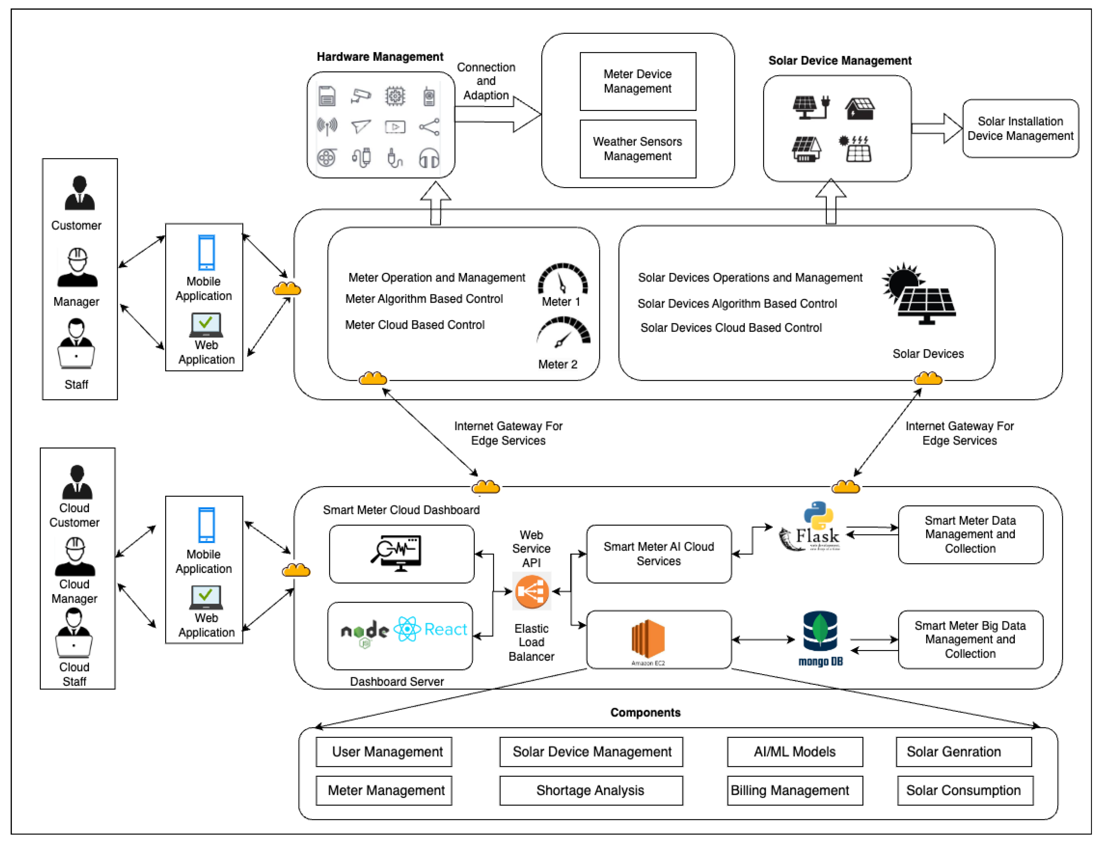
3. Electricity Management System Design

After model development, researchers also developed a system on AWS cloud, initiated deployment process, and developed a web interface to visualize the data. This system was divided into several components: server maintenance, supporting frameworks, hardware management, database management, model development, and user interface.

3.1. System Architecture

Figure 1 illustrates the system architecture, which comprises major components from both hardware and the cloud user. The major components of the system architecture include hardware elements, such as servers and storage devices, which form the infrastructure for data processing and storage. Additionally, the cloud component of the system architecture provides scalability, flexibility, and accessibility for the data-driven green energy model. It allows for the seamless integration of diverse models and facilitates system deployment across multiple locations.

Figure 1. System architecture.

Hardware management focuses on smart meter configuration and solar device management. Cloud-based management of hardware devices helps manage operations and configurations. Hardware devices are connected to the cloud using edge internet services. Edge internet services enable remote access to the data and allow for remote monitoring and system analytics. Additionally, edge internet services provide a secure connection to hardware devices.

The two components, meters and solar devices, are monitored using dashboards deployed on the cloud. Users can access various components of the system, such as admin-based control of solar devices, meters, and AI models for predicting short-term shortages, consumption, and power generation.

3.2. Cloud AI

Cloud AI services provide users with data analysis and visualization capabilities. This allows them to make informed decisions about power usage and generation. Users can also access the system’s customer portal to view their energy usage and manage their bills. The developed models were deployed and used on the server. The staff level has access to the system’s data to monitor and analyze customer energy usage, identify potential issues, and make recommendations for improvements. The AI models help the staff and users to automate processes and optimize energy usage.

3.3. Front End

Frontend services provide an intuitive, user-friendly interface, making it easier for staff to access and use the system. The AI models detect and respond to any abnormalities in the data, providing further insight into the customer’s energy usage. The resultant predictive data are used to develop a user interface using the Flask framework on the frontend. The interface is made accessible to end-users, allowing them to look through the dashboard and make well-informed decisions based on the analysis of predicted generation, consumption trends, and energy shortage projections. The interface also allows customers to set custom alerts and notifications based on their preferred energy usage settings. The interface is regularly updated with the latest data and trends, ensuring that users are always informed and up-to-date.

Figure 2 refers to the user consumption dashboards for meters.

Figure 2. User interface showing meter usage for past 30 days.

A comparison of the meters’ actual and predicted solar generation is shown in Figure 3. The date range can be customized to be able to check the prediction at different levels according to the measurements. The deployed models were used to make the predictions.

Figure 3. User Interface for Meter Solar Generation.

Users can examine the average electricity generation for certain devices in Figure 4, and a comparison of actual and anticipated generation is shown in Figure 5. These visualizations facilitate improved evaluation of solar meter performance by offering a thorough summary in addition to aiding in the monitoring of generation patterns.

Figure 4. User interface for meter solar generation.

Figure 5. User interface for meter solar generation.

Figure 6 shows how to setup the configuration and check the devices’ status using the meter device management page.

Figure 6. User interface for meter management.

Figure 7 illustrates the shortage forecast in which users are informed on whether they should buy, sell, or hold the generated electricity, based on what the model’s shortage prediction tells us. The shortage forecast is based on the current demand, expected demand, and available electricity. The forecast is also adjusted to take into account any changes in weather or other factors that could influence the demand for electricity. Finally, the forecast is updated regularly to ensure that it accurately reflects the situation.

Figure 7. User interface for shortage prediction.

3.4. Database

MongoDB was used in conjunction with Flask to process and display data pertaining to solar generation, energy consumption, and meter statuses as well as handling and displaying other data. It was a perfect fit for this project because of its advanced querying and indexing features, which were vital in managing the large volumes of regularly updated data. Important parameters such as timestamps, energy consumption expressed as kWh, estimated load values, and detailed meteorological information, such as temperature, relative humidity, dew point, cloud cover, and wind speed have all been included in the analysis. In the same way that energy output, anticipated generation, and environmental considerations were examined, solar generating data were also thoroughly analyzed. Using this comprehensive dataset, a detailed data analysis was performed to aid in decision-making. For instance, by correlating energy consumption with meteorological data, it became easier to accurately predict future energy needs and adjust generation strategies accordingly. In Romania, every meter had a unique number, such as “ABR-SG-001” for the solar meter at “Campus Building ABR-SG”. Information about the cloud status, working status, and active status of the meter were included in this report. It provided insight into the environmental conditions that can affect solar energy production by providing information about cloud status. Solar panels can produce less energy when cloud cover reduces the sunlight reaching them. Thus, to maintain optimal performance, energy consumption and generation strategies were adjusted based on cloud status. To facilitate real-time analytics, it kept separate collections for solar generation, meter performance, and consumption. If any abnormalities or discrepancies in the data are identified, the system provides alerts and notifications. By taking prompt action, the operators can avoid any potential losses. Figure 8, Figure 9 and Figure 10 are the samples of the dataset stored in each record.

Figure 8. Solar generation data sample.

Figure 9. Consumption meter data sample.

Figure 10. Shortage prediction after model implementation.

4. System Use Cases

4.1. Use Case 1: Making Data-Driven Decisions

By integrating AI into the cloud, the system can be used to handle emergency situations such as natural disasters, power outage, and blackouts by making data-driven decisions.

The system uses historical disaster records and weather data in order to make data-driven decisions to effectively handle emergencies such as natural disasters, power outages, etc. The shortage model can help the user effectively manage their energy during these emergencies. In the shortage analysis page, the user can use the application to display the predicted shortage produced from the reinforcement model, as well as the actual shortage. The page also shows a graph of predicted shortage versus time; for each hour, the user is able to analyze the predicted shortage values, allowing them to make well-informed decisions to balance generation and consumption. The data from the shortage model give real-time insights into how well the user is storing their energy, making it invaluable for handling emergencies. This leads to the development of a resilient community which can be prepared for emergencies that lead to a severe energy shortage.

4.2. Use Case 2: Managing System Hardware

Staff are able to add/delete meter information in the system, which will be updated in real time in the MongoDB, allowing the system to have a real-time analysis of current meter data. They are able to input different information to each individual meter such as device name, location, deployment date, etc. There is also an option to delete the meter from the system if needed. This system allows for the meter information to stay updated at all times, and for users to continue receiving accurate and live information from the system.

4.3. Use Case 3: Consolidated Dashboard for Generation, Consumption, and Shortage Analysis

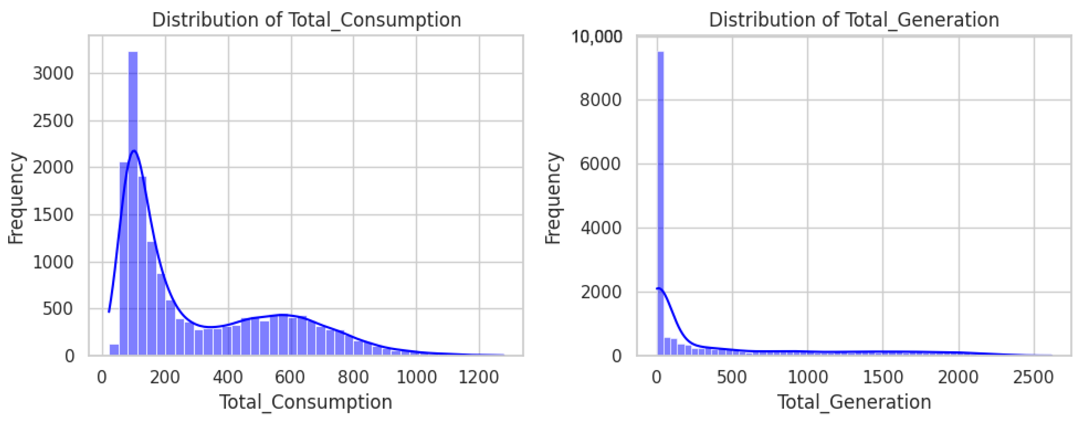
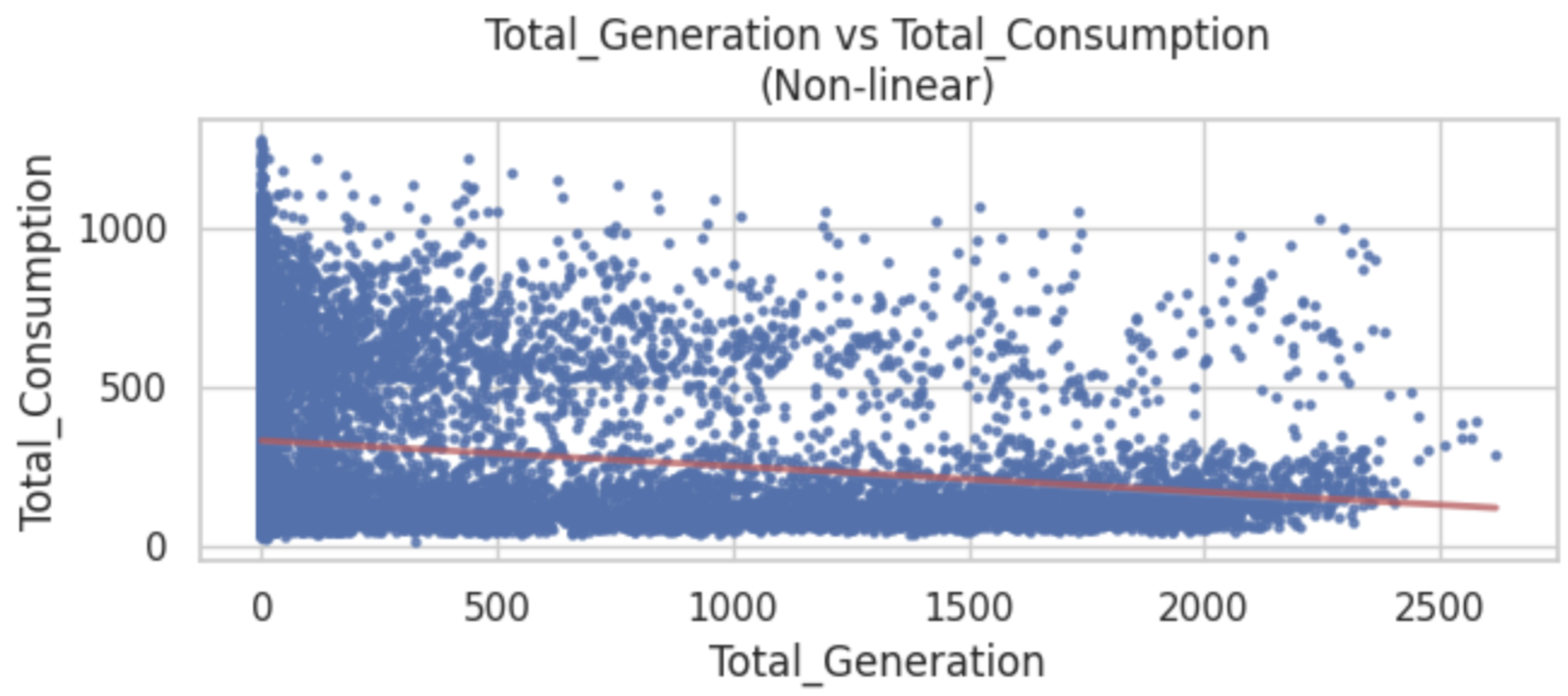
The home page shows the user details of the electric meter and solar meter, as well as IoT. It tells the user how many working meters there are, as well as the max usage for each meter in the last 30 days. Additionally, a visualization of the load consumption and solar generation are displayed, with a separate line for each meter. There is also a map of the location of the meters; in this paper’s scenario, the meters are located in Romania. Thus, users can view the consumption and generation data of the campus meters, status of meters, location of meters, etc., all on the same dashboard, giving them a clear overview of the meter usage for the past 30 days. The system allows users to view all relevant meter data through an appealing and coherent dashboard.

Users are also able to analyze their actual and predicted values of load consumption and solar generation for their desired meters on the same page. Once they input the date ranges and meters they want to analyze, the system shows the user two graphs: one depicting the actual values of the solar generation for each meter over time, and another comparing the actual and predicted aggregated values of the solar generation over time. Clicking on each point on the graph gives the numerical values of the consumption/generation, allowing for the user to perform a deeper analysis if needed. The shortage analysis page also allows users to analyze their actual and predicted electricity shortage.

By showing real-time visualizations and detailed data analysis on a consolidated dashboard, users are presented with a centralized overview of critical energy data. Having all these key metrics on a dashboard can help users make faster and well-informed decisions. It also simplifies data access, saving time and reducing the risk of errors from switching between multiple systems.

5. Data Engineering

5.1. Data Collection

The main challenge was choosing the intervals for data collection, and the second challenge was to connect the data to the cloud with APIs to obtain real-time data. The models used data collected from the E-LAND CO2 reduction in the Valahia University of Targoviste (UVTgv) [43], Photovoltaic Geographical Information System (PVGIS) [44], and Open-Meteo [45]. Since the area has heavy rain, winds, and substantial seasonal temperature changes, it is an ideal choice for this research because of the availability of multiple weather and solar radiation factors. There were a total of three solar panels installed at different buildings of the UVTgv green campus, namely Romania, ICSTM, C and ABM buildings, and data were extracted every 60 min. The collected data were stored in Google Cloud Platform (GPC). The data files were housed in a specialized bucket created within Google Cloud Storage (GCS). This bucket was established within the US-Central (Iowa) region, primarily chosen for its accessibility and cost-efficiency.

5.2. Data Pre-Processing

Data cleaning was an important part of data preparation since the data were coming from three different sources and had to be consolidated to be analyzed. After consolidating the data, data sanitization steps such as checking for duplicates, outliers, null values, and aligning the data were performed. The consolidated CSV shows time, generation readings, consumption readings, weather data, and solar parameters. Table 6 shows the time, generation readings, and consumption readings after cleaning from three buildings. Generation readings of “0” indicate it is night time and there is no solar energy generated.

Table 6. Sample data columns 1–10.

Time	Day	Month	Hour	Con1	Con2	Con3	Gen1	Gen2	Gen3
1/1/19 0:30	1	1	0	263.93	119.97	100.38	0	0	0
1/1/19 1:30	1	1	1	261.38	128.87	98.78	0	0	0
1/1/19 2:30	1	1	2	289.59	130.39	129.99	0	0	0
1/1/19 3:30	1	1	3	340.86	143.53	129.51	0	0	0
1/1/19 4:30	1	1	4	399.54	174.59	150.48	0	0	0
1/1/19 5:30	1	1	5	359.57	251.32	135.99	0	0	0
1/1/19 6:30	1	1	6	352.05	247.05	147.60	0	0	0
1/1/19 7:30	1	1	7	344.88	239.04	147.82	0	0	0
1/1/19 8:30	1	1	8	329.57	237.91	135.97	14.36	254.63	17.34
1/1/19 9:30	1	1	9	314.84	230.92	129.75	70.62	644.55	85.29

Table 7 shows weather data, and the solar parameters were the following:

Table 7. Sample data columns 11–20.

G(k)	G(d)	G(t)	Temp (°C)	Humidity (%)	Dew Point (°C)	Precip (mm)	Cloud Cover (%)	Cloud Class	Wind Speed (m/s)	Total Gen
0	0	0	0.31	87	−1.7	0	94	Overcast	7.2	486.9927752
0	0	0	0.24	88	−1.6	0	94	Overcast	5.6	830.8305377
0	0	0	0.21	88	−1.5	0	94	Overcast	5.8	533.8596574
0	0	0	0.32	88	−1.5	0	94	Overcast	5.6	818.1938571
0	10.29	0.56	0.56	91	−2.5	0	91	Overcast	5.5	744.5520956
0	19.37	1.44	0.05	91	−2.1	0	67	Mostly Cloudy	5.1	746.8227593
0	75.57	2.86	−0.15	91	−1.9	0	94	Overcast	4.2	828.5234751
0	79.57	3.85	0.42	91	−1.9	0	94	Overcast	4.2	697.6937879
0	77.69	2.92	2.32	77	2.23	0	94	Overcast	4.6	606.5127888

• Gb(i): Beam irradiance on the inclined plane (plane of the array) (${\mathrm{W/m}}^2$).
• Gd(i): Diffuse irradiance on the inclined plane (plane of the array) (${\mathrm{W/m}}^2$).
• Gr(i): Reflected irradiance on the inclined plane (plane of the array) (${\mathrm{W/m}}^2$).

For predictive modeling using historical data, it was important to have the same date format for modeling purposes, which made data standardization an important step. The date and interval column in the dataset were used to create a date timestamp column which replaces both those columns. Moreover, the extraction of details like the day of the week, month, or year from the date is essential; hence, a feature engineering process was conducted. This procedure facilitates the development of new features, enhancing the robustness of the analysis and modeling process by adding a layer of valuable information like day of week, month, and hour of day, which is extracted from the new date timestamp column. Having successfully formatted the data, the distribution of target variables was checked—“Total Consumption” and “Total Generation”—as well as their relationship presented in Figure 11 and Figure 12. In the figures, frequency refers to the amount of times that numerical consumption and generation values appeared in the datasets. In Figure 11, the histogram is smoothed to make the data’s underlying distribution easier to visualize. Kernel Density Estimation (KDE) curves appear in blue in the histograms.

Figure 11. Target variables’ data distribution.

Figure 12. Target.

In Figure 12, an overall correlation between Total_Generation (on the x-axis) and Total_Consumption (on the y-axis) is illustrated by a red line in the graph that illustrates a non-linear regression trendline. With an increase in Total_Generation, Total_Consumption tends to decrease slightly, but there is considerable variability.

5.3. Training Data Preparation

Data analysis was conducted on 17,520 rows and 22 columns after pre-processing and cleaning two years’ worth of data. The dataset was split 80:10:10 into training, testing, and validation, respectively, during the model development process. Using the validation data, the hyperparameters of the models developed were finetuned using the training data.

Table 8 shows the summary of the size of the dataset after every stage in the data engineering process.

Table 8. Size of dataset after every stage in data engineering process.

Stage	Action Performed	Rows × Columns
Pre-Raw Data Collection	Extraction of Solar power data for 2019 and 2020	17,520 × 11
	Extraction of Radiation data for 2019 and 2020	17,520 × 8
	Extraction of Weather data for 2019 and 2020	17,520 × 23
Pre-Processing	Compiling solar power, radiation, weather data, removing unwanted columns, date formatting, feature extraction, and checking for null values and outliers.	17,520 × 20
Transformation	Converted the cloud cover column from numerical values to categorical values.	17,520 × 20
Data Preparation	Training dataset	13,104 × 20
	Test dataset	2208 × 19
	Validation dataset	2208 × 19

6. Model Development

The system forecasts consumption, generation, and shortage using three different approaches. The first approach uses various traditional and novel ML model approaches to predict electricity consumption, generation, and shortage values. As a second approach, this research aggregated data from all three buildings to forecast the total energy consumption and generation for the entire campus. As a third approach, a distributed training approach was employed, in which the best models found from Approach 1 are used to train the distributed data coming from each source. This research aims to develop a robust decision-making model for the campus that combines the results from energy generation machine learning, consumption machine learning, and shortage decision-making models so that users can make well-informed decisions to balance energy usage. Working with the various models described above required the use of a computer that has sufficient hardware to handle the processing needs of training and testing these models. Specifically, a local desktop/laptop with 16 GB RAM, multi-core processor, 29 graphic card of 1 GB, and SSD storage for the dataset was used. This project implementation also required Google Cloud Platform to keep the data in the cloud and for the execution, and it required a laptop/desktop with a multi-core processor with at least 8 or 16 GB RAM to speed up the training execution. For the data analysis preparation, a local Python Jupyter Notebook: v3.11 was used and in the Google Cloud Platform, and Big Query was used. It required Pandas, NumPy, matplotlib SciKit-learn, and seaborn libraries to perform data analysis and data visualization. In addition to this, the implementation of the deep learning models required the Tensor Flow, Keras, and PyTorch libraries.

Figure 13 shows the detail flow and overview of the model’s operation.

Figure 13. Overview of campus-oriented hierarchical model.

6.1. Approach 1: Traditional Models

6.1.1. Long Short-Term Memory (LSTM)

LSTM is highly suitable for the green energy project due to its proficiency in handling time-series data, such as energy consumption patterns and solar production. LSTM’s ability to learn from historical data enables accurate forecasting of energy demand and supply. The architecture of the LSTM model consists of 50 units with a ReLU function, followed by a Dense layer with one unit for regression. Training the LSTM model involved 50 epochs, a batch size of 32, and parameter tuning using validation data. The model was monitored for improvement using the validation loss, with early stopping activated after 10 patience epochs to prevent overfitting. After training was completed, predictions were generated for the test set, and the model’s performance was evaluated. LSTM was used for short-term consumption forecasting and short-term generation forecasting on an hourly basis in this study based on the existing research by [6,7,30] to forecast electricity consumption and [19,20,22,25,27,28,30] to forecast solar generation. However, in this study, it was found that LSTM performed poorly with consumption and generation predictions, with MAEs of 22.20 and 82.17 for consumption and generation predictions, respectively. This poor performance could be attributed to the complex and nonlinear nature of the data, which LSTM may struggle to model accurately.

6.1.2. Convolutional Neural Network (CNN)

CNNs are specifically designed for processing and analyzing structured grid-like data as well as sequential data, making them applicable to energy consumption analysis. The key operations within a CNN include convolution, activation, pooling, and fully connected layers. The convolution layer applies filters (kernels) to the input data. After each convolutional operation, an activation function is applied to introduce nonlinearity to the model. This is followed by applying a pooling layer to reduce the spatial dimensions of the data. The network ends with one or more fully connected layers, making predictions based on learned features. In the context of time series data, the architecture can be adapted to 1D or 2D structures to process the sequential data effectively. CNNs automatically extract relevant features from the sequential energy data and identify complex patterns and relationships between various factors impacting energy consumption, such as time, weather conditions, community events, and historical usage patterns. It also excels at recognizing localized patterns within the data, which could represent specific trends or events influencing energy usage within the campus. A CNN was used in this study as a similar technique to LSTM for predicting short-term consumption and short-term generation based on existing research by [8,10] to forecast load consumption and [22,28] to forecast solar generation. Surprisingly, the results were worse than LSTM when predicting both short-term consumption and short-term generation. The MAE for consumption was 24.76, and the MAE for generation was 94.97.

6.1.3. Support Vector Regressor (SVR)

After experimenting with popular deep learning models, SVR was tested. Support vector regression is a form of support vector machines, and applies the principles of SVM, a machine learning method used for classification and regression, to predict continuous outcomes. Electric consumption data often exhibit nonlinear patterns due to various factors like weather, time of day, and economic activities. Thus, SVR is good for this task due to its ability to handle nonlinear data. To predict the continuous values, it aims to find the best fitting line. SVR is distinguished using an epsilon margin of tolerance, and it works especially well with nonlinear data due to the work of kernel functions. By attempting to be as flat as feasible and minimizing error within this margin, the method strikes a balance between the model’s predicted accuracy and complexity. Emphasizing the optimization of hyperparameters, a grid search was conducted to explore the ‘C’ (regularization parameter) and ‘epsilon’ (insensitivity parameter) space. The grid search process revealed the best hyperparameters for SVR to be ‘C’: 10, ‘epsilon’: 0.1. Existing research by [12] used SVR to forecast load consumption and [19,21] used SVR to forecast solar generation. Aligning to the existing research, this research also used SVR to forecast short-term consumption and generation. As compared to LSTM and CNN, the MAE of SVR for consumption was worse than 29.39, whereas the MAE for generation was improved to 52.84.

6.1.4. Random Forest Regressor (RFR)

RFR was also experimented with in this research. The Random Forest Regressor operates within the domain of ensemble models, integrating the outcomes of numerous decision trees, thereby enhancing the overall accuracy of predictions. Each decision tree is constructed using a random subset of the training data and a bootstrapped subset of features. This diversification diminishes the correlation between individual trees and decreases the variance in predictions, resulting in higher accuracy and mitigating the risks of overfitting. In the pursuit of optimizing the Random Forest model for short-term energy consumption prediction, an exhaustive hyperparameter tuning process was conducted. The grid search spanned various combinations of ‘n_estimators’ (number of trees in the forest) and ‘max_depth’ (maximum depth of each tree). The best-performing hyperparameters, as determined by the negative mean squared error on a 5-fold cross-validation, were found to be ‘max_depth’: 10 and ‘n_estimators’: 150.

Existing research by [19,21] used RFR to forecast solar generation. But this research used RFR to forecast both short-term consumption and generation. It was found that, with the help of RFR, the performance of the models was significantly improved, and the models were able to achieve an MAE of 14.33 for consumption and 39.54 for generation after using RFR. This improvement can be attributed to the Random Forest Regressor’s ability to handle nonlinear relationships and interactions between variables more effectively.

6.1.5. Extreme Gradient Boosting (XGBOOST)

This paper also experiments with XGBoost based on existing research by [25] to forecast solar generation. With XGBoost, it is possible to capture generation patterns of solar panels due to its ability to handle complex nonlinear relationships and interactions between features. By combining multiple weak models into a strong predictive model, boosting is an ensemble learning technique. As a result, XGBoost is able to capture intricate patterns and dependencies in the data, thereby allowing it to accurately predict the solar panel generation and the load consumption as a result. In the same way as SVR and RFR, XGBOOST was used to forecast short-term consumption, and generation.As compared to all the models in all the sections, the model in this section performed the best. The MAE was 11.67 for consumption and 39.12 for generation, which is close to Random Forest. XGBoost performed the best in this experiment due to its robust handling of nonlinear relationships and interactions between features, which are critical in accurately modeling solar panel generation and load consumption. Its ability to effectively minimize overfitting while maintaining high predictive accuracy contributed to its superior performance. Additionally, its efficient computational speed allowed for quicker model training and evaluation. A hyperparameter tuning process was conducted using a predefined grid for ‘n_estimators’ (number of trees), ‘max_depth’ (maximum depth of each tree), and ‘learning_rate’ (step size shrinkage). Following a comprehensive grid search, the optimal hyperparameters for XGBoost were identified as ‘learning_rate’: 0.05, ‘max_depth’: 5, ‘n_estimators’: 100.

6.1.6. Shortage Forecasting Model Development

The campus model is developed for communities from various sectors and locations. The shortage forecasting model, or campus model, helps users make the decision to buy/sell or hold the electricity based on an analysis from consumption and generation forecast. This research experiments with three methods: prediction, classification, and a novel mathematical approach. The background models used are SVR, RFR, CNN, and XGBOOST.

To predict shortages, this research used the SVR, XGBoost, and Random Forest models. The prediction model forecasts future shortage values based on using historical shortage values to train the model.

To classify shortages, the models consist of Neural Networks, SVM, and Random Forest based on the features of the data. The classification model uses historical shortage values to predict the severity of the future shortages (i.e., low severity, high severity).

Using the novel mathematical approach to predict the value of shortage units, the predicted solar generation is subtracted from the solar consumption for each sequential hour as presented in Equation (1).

$$M=\sum _{i=1}^n(S{G}_i-S{C}_i)$$

(1)

where n represents the number of hours, $SG$ represents solar generation value, and $SC$ represents solar consumption value.

By subtracting the most accurate predicted generation values from the most accurate predicted consumption values, the model is expected to predict the most accurate shortage value.

Reinforcement learning was used to enhance the models via Q-learning and state-action-reward-state-action (SARSA). Q-learning involves estimating the value of taking specific actions in given states, and updating these values using the action that maximizes future rewards, while SARSA directly evaluates the actions the agent takes, and the subsequent actions it takes. At each time step, the agent observes the current state, which corresponds to a specific data point in the dataset, and selects an action that predicts the shortage value for that data point. The action is chosen based on the agent’s policy, which is learned through Q-learning. The predicted generation value is obtained from the XGBoost model trained on the dataset. The environment provides feedback to the agent in the form of rewards, which are based on the accuracy of the predicted generation values compared to the true values. The agent’s objective is to maximize cumulative rewards over time by learning an optimal policy that guides its actions towards accurate generation predictions. Through trial and error, the agent learns to improve its predictions by adjusting its policy based on the observed rewards and experiences in the environment.

6.2. Approach 2: Aggregated Training Learning Models

The primary focus of the project was to accurately predict energy consumption and generation for the entire green campus. Thus, by utilizing the robust XGBoost algorithm, which was selected for its superior performance, an aggregate model was first constructed. Utilizing the mathematical approach described above, this model synthesized data from the entire campus, encompassing all three buildings to forecast the total shortage, as seen in Equation (2).

$$TotalShortage=\sum _{i=1}^n\left(ShortageValue\right)$$

(2)

Table 9 shows a snippet of the predicted values based on hourly basis of consumption, generation, and shortage using the aggregated approach.

Table 9. Predicted values from aggregated approach.

Timestamp	Forecasted Consumption	Forecasted Generation	Predicted Shortage	Status	Action
2020-12-01 08:30:00	662.52	605.46	57.05	Shortage	Buy
2020-12-01 09:30:00	638.81	1103.60	−466.79	Abundance	Sell/Store
2020-12-01 10:30:00	638.08	1293.91	−655.10	Abundance	Sell/Store
2020-12-01 11:30:00	607.37	1248.24	−640.87	Abundance	Sell/Store
2020-12-01 12:30:00	595.18	1366.72	−771.54	Abundance	Sell/Store
2020-12-01 13:30:00	591.22	995.87	−404.64	Abundance	Sell/Store
2020-12-01 14:30:00	603.97	525.48	78.49	Shortage	Buy
2020-12-01 15:30:00	615.02	84.83	530.14	Shortage	Buy
2020-12-01 16:30:00	647.05	2.21	644.84	Shortage	Buy
2020-12-01 17:30:00	657.33	2.21	655.12	Shortage	Buy

6.3. Approach 3: Distributed Training Learning Models

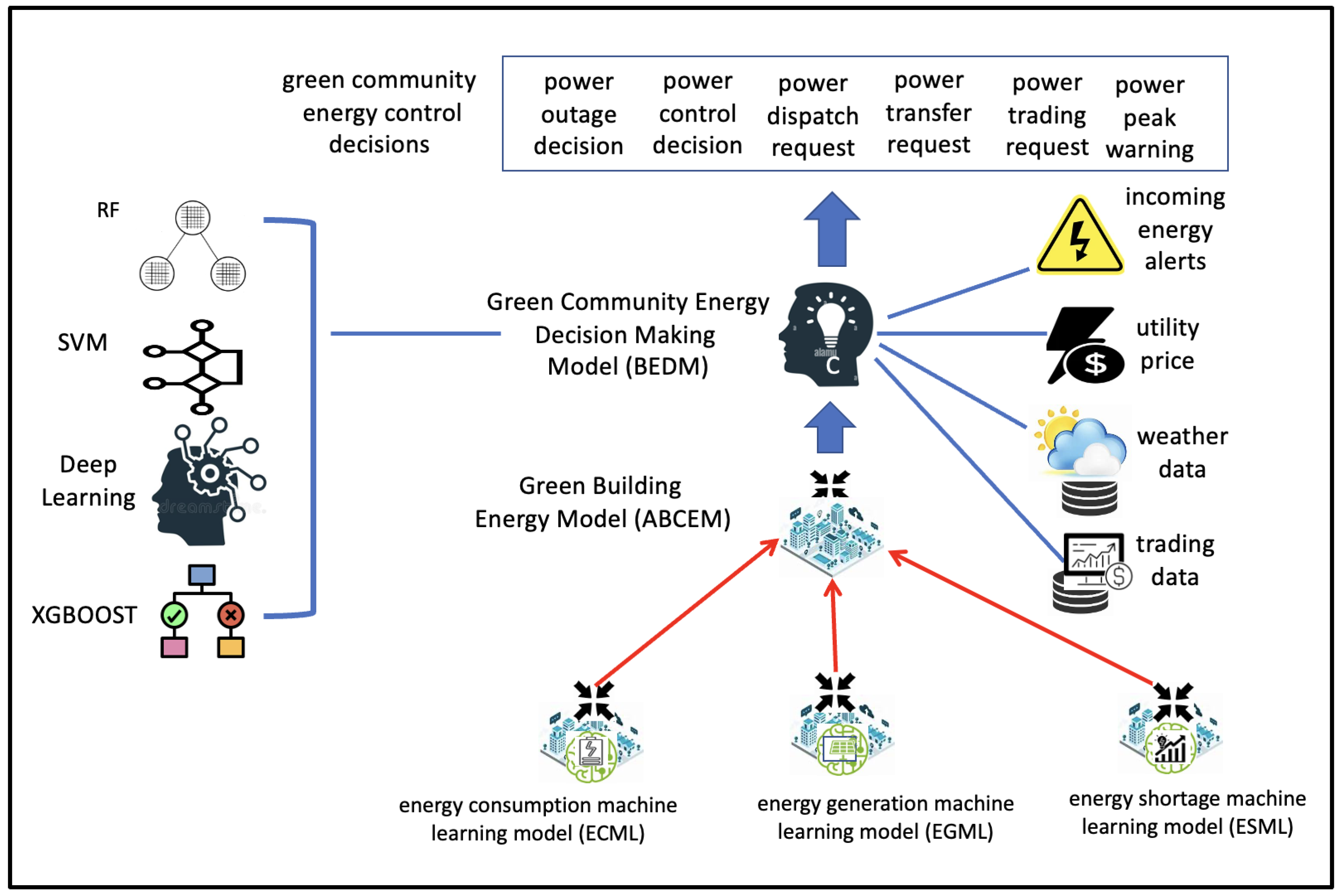
Following the creation of the aggregate model, individual predictive models for each building were developed to gain a more granular understanding of energy dynamics within the community. These models were tailored to account for the unique consumption and generation patterns of each building.

7. Decision-Making

Once accurate shortage prediction values were obtained, consolidated results were found using Equation (3) to form a decision on what the user should do.

$$D_1={\displaystyle \frac{S{B}_1}{S_{\mathrm{total}}}}{D}_2={\displaystyle \frac{S{B}_2}{S_{\mathrm{total}}}}{D}_3={\displaystyle \frac{S{B}_3}{S_{\mathrm{total}}}}$$

(3)

where $S{B}_1,S{B}_2,S{B}_3$ represent the predicted shortage of each building, $S_{\mathrm{total}}$ is the sum $S{B}_1+S{B}_2+S{B}_3$, and $D_1,D_2,D_3$ represent the fraction of the total campus shortage that Building 1, 2, and 3, contribute to, respectively. Using these fractions, the model outputs a cohesive decision (buy, sell, or hold). After obtaining decisions for each building, distributed and aggregated training were implemented to further enhance the community-based model in forming a final decision.

7.1. Distributed Decision-Making

The individual components of the distributed decision model system operate independently, but are part of a larger centralized system. Each of these local energy management systems (EMSs) processes data and produces outputs locally. Specifically, each meter used a machine learning model to forecast load consumption and solar generation for each meter based on historical data and various weather conditions. Then, each building produces a distinct decision based on the values of $D_1,D_2,D_3$, as calculated in Equation (3). Figure 14 gives a detailed flow of a working distributed model.

Figure 14. Distributed model for community-level decision-making.

7.2. Aggregated Decision-Making

In an aggregated decision model, data from multiple communities are consolidated into a unified system. The proposed campus model utilizes this, combining data from multiple meters, allowing users to view consolidated output data for multiple meters on campus. The aggregated model structure is useful to users when they want to look at the campus on a large scale and ensure overall campus energy stability. Figure 15 gives a detailed flow of a working aggregated model.

Figure 15. Aggregated model for community-level decision-making.

To obtain aggregated model results, the results of $D_1,D_2,D_3$ obtained from Equation (3) were added and divided by 3. Using the aggregated decision obtained from Equation (4), the system is able to come to a final decision for the whole campus.

$$AggregatedDecision={\displaystyle \frac{D_1+D_2+D_3}{3}}$$

(4)

8. Results

The system gave comparatively better results than most existing research. This paper’s unique mathematical approach for training the models, combined with reinforcement learning, improved results. For final decision-making, better results were gained from aggregated models.

Several metrics were used to assess the performance of the models when forecasting energy generation, consumption, and shortage values. These metrics included mean absolute error (MAE) and root mean square error (RMSE). MAE provides a straightforward measure of the average magnitude of errors in predictions, calculating the average of the absolute differences between predicted and actual values. RMSE also measures the differences between predicted and observed values, calculating the square root of the average of the squared differences between predicted and actual values. Together, these metrics offer a comprehensive evaluation of the model’s performance in accurately forecasting energy trends. In the following are consolidated results from all the phases of model development and system output. In most cases, the model outputted the best results from XGBOOST followed by RF. A common threshold used to decide whether the model is behaving well is an RMSE of under 50 and an MAE of under 25. The Table 10, Table 11 and Table 12 present consolidated results.

Table 10. Traditional model performance for various components (RMSE and MAE are reported in kilowatts).

Component	Models	RMSE	MAE
Generation	XGBoost	94.4	39.12
	RF	100.28	39.54
	SVM	116.44	52.84
	LSTM	158.58	82.17
Consumption	XGBoost	14.65	11.67
	RF	18.08	14.33
	SVM	43.77	29.39
	LSTM	31.67	22.2
	CNN	37.21	24.76
Shortage Prediction	XGBoost	79.08	45.88
	RF	86.47	48.97
	SVR	147.34	74.17

Table 11. Model performance for shortage classification.

Model	Accuracy	Correct Prediction	Incorrect Prediction
RF	91.44%	673	63
NN	89.40%	658	78
SVM	88%	652	84

Table 12. Model performance for distributed and aggregated training (RMSE and MAE are reported in kilowatts).

Component	Training Type	Models	RMSE	MAE
Generation	Distributed	Building 1	53.15	26.32
		Building 2	42.08	21.59
		Building 3	30.25	18.74
	Aggregated	Aggregated Model	75.45	33.12
Consumption	Distributed	Building 1	34.43	32.06
		Building 2	14.96	12.46
		Building 3	1.12	8.57
	Aggregated	Aggregated Model	14.72	12.00

The effectiveness of the classification model was calculated based on the percentage accuracy with which it could predict the severity of the shortage.

Because of the high margins of error in the original shortage model, reinforcement learning was incorporated into the shortage model in order to further improve it. This research calculated the accuracy of the model’s shortage analysis by dividing the total number of correct instances with the total number of instances. To do this, the number of rows with correctly identified positive values (actual shortage and predicted shortage both being positive), correctly identified negative values (actual shortage and predicted shortage both being negative), and mixed counts (actual shortage value and predicted shortage value having different signed values) were counted. This model achieved an accuracy of 98.2% using the following calculation presented in Figure 16.

Figure 16. Reinforcement learning results for shortage analysis with mathematical approach.

Runtime performance was also an important metric, as it is crucial for meeting system response time targets. Regarding consumption load prediction, the system had a runtime of 0.175 s; additionally, the integration timing for UI interaction, including data retrieval from MongoDB and display to the user, is approximately 4 s. Regarding solar generation prediction, the system had a runtime of 0.47 s; the integration timing for UI interaction took approximately 5 s. Finally, regarding shortage prediction, the system had a runtime of 0.5 s; the integration timing for UI interaction took 5 s. Analyzing these runtime factors helps in optimizing system responsiveness and user experience. According to the results, the developed system is robust and takes into account various important parameters and aspects of training. Additionally, this research has implemented advanced techniques for managing emergency situations such as shortages at the community level. It is worth noting that, 98.2% of the time, the campus model is effective at predicting shortages, resulting in higher accuracy. Additionally, any industry working on shortage forecasting can easily use this system.

9. Conclusions

From various aspects, this research has implemented a system that is highly conducive to sustainable development. With this system, it is possible to accurately forecast the three major elements of green AI services: energy consumption, energy generation, and energy shortages. Using this system, a community can efficiently manage its electricity needs. This satisfies the ultimate goal of this system: to improve energy sustainability among smart communities through the use of sophisticated, data-driven insights.

The research used data from three different sources to design the system, and data were fed into machine learning, deep learning, and embedded models for experiments. Two advanced methods (distributed, aggregated) were used to train the data in this system, which produced better results. These aggregated and distributed models were ultimately applied in the system. For developing the models and managing the data, this system used Python v3.11, Flask v3.1.0, and MongoDB v5.3. The system’s frontend was developed using NodeJs and React framework for displaying real-time graphs such as electricity load graphs, metered data, solar generation graphs, and shortage predictions graphs. The system’s backend was primarily developed using Javascript v2.11.0 in Visual Studio Code v1.92. The system was then tested for accuracy and performance. Regarding electricity generation modeling, XGBoost produced an RMSE of 94.4 kW and an MAE of 39.12 kW, which was significantly lower than the other models. Regarding electricity consumption modeling, XGBoost produced an RMSE of 14.65 kW and an MAE of 11.67 kW, which was more accurate than other models. Finally, regarding shortage, XGBoost had an RMSE of 79.08 kW and an MAE of 45.88 kW. However, even with XGBoost, the models had high margins of error; thus, reinforcement learning was implemented into the models. This greatly improved accuracy, and the shortage model improved to an accuracy of 98.2 %. Additionally, the quick runtime, with all models running in less than 5 s, suggests that the system is extremely applicable in real-time applications. The important components of the system like frontend, backend, and models were neatly designed and implemented with reliable technologies. The results were satisfactory and the system is now ready for deployment.

In conclusion, the system’s performance, accuracy, and integration capabilities make it a promising project and a reliable choice for users.

Future Works

Price Prediction Component: In the future, real-time analysis and additional data can be gathered for price prediction. To enhance the accuracy of price-prediction models, the integration of machine learning algorithms that analyze historical price data and market trends should be considered. Additionally, incorporating external factors such as economic indicators, news sentiment analysis, and competitor pricing can provide more comprehensive insights. Regularly updating and validating the models with new data will also help maintain their accuracy over time.

Cyber Green energy System Infrastructure: A stronger and secure cloud-based infrastructure is needed to support big data. In order to manage trading data, it is imperative to collect, monitor, drive, and analyze it. Data on energy consumption and production should be collected, managed, and analyzed using cloud infrastructure. The cloud-connecting infrastructure allows users to connect multiple cloud-based infrastructures. For green AI to be more effective and secure, cloud-based infrastructure must be developed. In this way, green system management will also become more affordable.

Incorporate Real-Time Data: To improve accuracy and responsiveness to changing weather conditions and their effects on solar energy output, enhance the project by integrating real-time data capabilities.

Frequent Model Updates: To keep prediction models current and accurate using the most recent data, it is crucial to establish a mechanism for regular updates and retraining.

References

1. Allied Market Research. Green Energy Market to Reach $2.4 Trillion, Globally, by 2032 at 8.9% CAGR: Allied Market Research. Cision PR Newswire, 11 December 2023. Available online: https://www.prnewswire.com/news-releases/green-energy-market-to-reach-2-4-trillion-globally-by-2032-at-8-9-cagr-allied-market-research-302011705.html (accessed on 11 December 2023).
2. Calero, I.; Cañizares, C.A.; Bhattacharya, K.; Baldick, R. Duck-Curve Mitigation in Power Grids With High Penetration of PV Generation. IEEE Trans. Smart Grid 2022, 13, 314–329. [Google Scholar] [CrossRef]
3. Powerwall. Tesla. (n.d.). Available online: https://www.tesla.com/powerwall (accessed on 13 June 2024).
4. Ahmad, A.; Javaid, N.; Mateen, A.; Awais, M.; Khan, Z.A. Short-term load forecasting in smart grids: An intelligent modular approach. Energies 2019, 12, 164. [Google Scholar] [CrossRef]
5. Bano, H.; Tahir, A.; Ali, I.; Khan, R.J.U.H.; Haseeb, A.; Javaid, N. Electricity load and price forecasting using enhanced machine learning techniques. In Innovative Mobile and Internet Services in Ubiquitous Computing; Springer International Publishing: Berlin/Heidelberg, Germany, 2020; pp. 255–267. [Google Scholar]
6. Bouktif, S.; Fiaz, A.; Ouni, A.; Serhani, M. Optimal deep learning LSTM model for electric load forecasting using feature selection and genetic algorithm: Comparison with machine learning approaches. Energies 2018, 11, 1636. [Google Scholar] [CrossRef]
7. Bouktif, S.; Fiaz, A.; Ouni, A.; Serhani, M.A. Multi-sequence LSTM-RNN deep learning and metaheuristics for electric load forecasting. Energies 2020, 13, 391. [Google Scholar] [CrossRef]
8. Estebsari, A.; Rajabi, R. Single residential load forecasting using deep learning and image encoding techniques. Electronics 2020, 9, 68. [Google Scholar] [CrossRef]
9. Guo, N.; Chen, W.; Wang, M.; Tian, Z.; Jin, H. Appling an improved method based on ARIMA model to predict the short-term electricity consumption transmitted by the Internet of Things (IoT). Wirel. Commun. Mob. Comput. 2021, 2021, 6610273. [Google Scholar] [CrossRef]
10. Kuo, P.-H.; Huang, C.-J. A high precision artificial neural networks model for short-term energy load forecasting. Energies 2018, 11, 213. [Google Scholar] [CrossRef]
11. Nepal, B.; Yamaha, M.; Yokoe, A.; Yamaji, T. Electricity load forecasting using clustering and ARIMA model for energy management in buildings. Jpn. Archit. Rev. 2020, 3, 62–76. [Google Scholar] [CrossRef]
12. Rai, S.; De, M. Analysis of classical and machine learning based short-term and mid-term load forecasting for smart grid. Int. J. Sustain. Energy 2021, 40, 821–839. [Google Scholar] [CrossRef]
13. Tong, C.; Li, J.; Lang, C.; Kong, F.; Niu, J.; Rodrigues, J.J.P.C. An efficient deep model for day-ahead electricity load forecasting with stacked denoising auto-encoders. J. Parallel Distrib. Comput. 2018, 117, 267–273. [Google Scholar] [CrossRef]
14. Ullah, F.U.M.; Khan, N.; Hussain, T.; Lee, M.Y.; Baik, S.W. Diving deep into short-term electricity load forecasting: Comparative analysis and a novel framework. Mathematics 2021, 9, 611. [Google Scholar] [CrossRef]
15. Zhang, J.; Wei, Y.-M.; Li, D.; Tan, Z.; Zhou, J. Short term electricity load forecasting using a hybrid model. Energy 2018, 158, 774–781. [Google Scholar] [CrossRef]
16. Mehta, Y.; Xu, R.; Lim, B.; Wu, J.; Gao, J. A Review for Green Energy Machine Learning and AI Services. Energies 2023, 16, 5718. [Google Scholar] [CrossRef]
17. BP Statistical Review of World Energy 2018. BP Statistical Review of World Energy 2018: Two Steps Forward, One Step Back,” bp Global. [Online]. Available online: https://www.bp.com/en/global/corporate/news-and-insights/press-releases/bp-statistical-review-of-world-energy-2018.html (accessed on 17 July 2024).
18. World Energy Outlook 2018. (n.d.). IEA. Paris, France, 2018. Available online: https://www.iea.org/reports/world-energy-outlook-2018 (accessed on 17 July 2024).
19. Mahmud, K.; Azam, S.; Karim, A.; Zobaed, S.; Shanmugam, B.; Mathur, D. Machine Learning Based PV Power Generation Forecasting in Alice Springs. IEEE Access 2021, 9, 46117–46128. [Google Scholar] [CrossRef]
20. Liu, C.-H.; Gu, J.-C.; Yang, M.-T. A Simplified LSTM Neural Networks for One Day-Ahead Solar Power Forecasting. IEEE Access 2021, 9, 17174–17195. [Google Scholar] [CrossRef]
21. Jebli, I.; Belouadha, F.-Z.; Kabbaj, M.I.; Tilioua, A. Prediction of Solar Energy Guided by Pearson Correlation Using Machine Learning. Energy 2021, 224, 120109. [Google Scholar] [CrossRef]
22. Zhou, H.; Liu, Q.; Yan, K.; Du, Y. Deep Learning Enhanced Solar Energy Forecasting with AI-Driven IoT. Wirel. Commun. Mob. Comput. 2021, 2021, 9249387. [Google Scholar] [CrossRef]
23. Babbar, S.M.; Lau, C.Y.; Thang, K.F. Long Term Solar Power Generation Prediction Using Adaboost as a Hybrid of Linear and Non-Linear Machine Learning Model. Int. J. Adv. Comput. Sci. Appl. 2021, 12, 536–546. [Google Scholar] [CrossRef]
24. Chodakowska, E.; Nazarko, J.; Nazarko, Ł.; Rabayah, H.S.; Abendeh, R.M.; Alawneh, R. ARIMA models in solar radiation forecasting in different geographic locations. Energies 2023, 16, 5029. [Google Scholar] [CrossRef]
25. Khan, W.; Walker, S.; Zeiler, W. Improved solar photovoltaic energy generation forecast using deep learning-based ensemble stacking approach. Energy 2022, 240, 122812. [Google Scholar] [CrossRef]
26. Atique, S.; Noureen, S.; Roy, V.; Subburaj, V.; Bayne, S.; Macfie, J. Forecasting of total daily solar energy generation using ARIMA: A case study. In Proceedings of the 2019 IEEE 9th Annual Computing and Communication Workshop and Conference (CCWC), Las Vegas, NV, USA, 7–9 January 2019; pp. 0114–0119. [Google Scholar] [CrossRef]
27. Kim, E.; Akhtar, M.S.; Yang, O.-B. Designing solar power generation output forecasting methods using time series algorithms. Electr. Power Syst. Res. 2023, 216, 109073. [Google Scholar] [CrossRef]
28. Lim, S.-C.; Huh, J.-H.; Hong, S.-H.; Park, C.-Y.; Kim, J.-C. Solar power forecasting using CNN-LSTM hybrid model. Energies 2022, 15, 8233. [Google Scholar] [CrossRef]
29. Maciejowska, K.; Nitka, W.; Weron, T. Enhancing load, wind and solar generation for day-ahead forecasting of electricity prices. Energy Econ. 2021, 99, 105273. [Google Scholar] [CrossRef]
30. Pan, C.; Tan, J.; Feng, D. Prediction intervals estimation of solar generation based on gated recurrent unit and kernel density estimation. Neurocomputing 2021, 453, 552–562. [Google Scholar] [CrossRef]
31. Kim, S.-G.; Jung, J.-Y.; Sim, M.K. A Two-Step Approach to Solar Power Generation Prediction Based on Weather Data Using Machine Learning. Sustainability 2019, 11, 1501. [Google Scholar] [CrossRef]
32. Hameed, Z.; Hashemi, S.; Traholt, C. Applications of AI-based forecasts in renewable based electricity balancing markets. In Proceedings of the 2021 22nd IEEE International Conference on Industrial Technology (ICIT), Virtual, 10–12 March 2021; Volume 1, pp. 579–584. [Google Scholar]
33. Bâra, A.; Oprea, S.-V. Intelligent system to optimally trade at the interference of multiple crises. Appl. Intell. 2023, 53, 25581–25604. [Google Scholar] [CrossRef]
34. Bottieau, J.; Hubert, L.; De Greve, Z.; Vallee, F.; Toubeau, J.-F. Very-short-term probabilistic forecasting for a risk-aware participation in the single price imbalance settlement. IEEE Trans. Power Syst. Publ. Power Eng. Soc. 2020, 35, 1218–1230. [Google Scholar] [CrossRef]
35. Essl, A.; Ortner, A.; Haas, R.; Hettegger, P. Machine learning analysis for a flexibility energy approach towards renewable energy integration with dynamic forecasting of electricity balancing power. In Proceedings of the 2017 14th International Conference on the European Energy Market (EEM), Dresden, Germany, 6–9 June 2017; pp. 1–6. [Google Scholar]
36. Jaehnert, S.; Farahmand, H.; Doorman, G.L. Modelling of prices using the volume in the Norwegian regulating power market. In Proceedings of the 2009 IEEE Bucharest PowerTech, Bucharest, Romania, 28 June–2 July 2009; pp. 1–7. [Google Scholar]
37. Santos, G.; Pinto, T.; Vale, Z.; Morais, H.; Praca, I. Balancing market integration in MASCEM electricity market simulator. In Proceedings of the 2012 IEEE Power and Energy Society General Meeting, San Diego, CA, USA, 22–26 July 2012; pp. 1–8. [Google Scholar]
38. Wang, Y.; Wang, J.; Zhao, G.; Dong, Y. Application of residual modification approach in seasonal ARIMA for electricity demand forecasting: A case study of China. Energy Policy 2012, 48, 284–294. [Google Scholar] [CrossRef]
39. Zhang, S.; Pandey, A.; Luo, X.; Powell, M.; Banerji, R.; Fan, L.; Parchure, A.; Luzcando, E. Practical adoption of cloud computing in power systems—drivers, challenges, guidance, and real-world use cases. IEEE Trans. Smart Grid 2022, 13, 2390–2411. [Google Scholar] [CrossRef]
40. Hong, T.; Pinson, P.; Wang, Y.; Weron, R.; Yang, D.; Zareipour, H. Energy Forecasting: A Review and Outlook. IEEE Open Access J. Power Energy 2020, 7, 376–388. [Google Scholar] [CrossRef]
41. Jaramillo, M.; Pavón, W.; Jaramillo, L. Adaptive Forecasting in Energy Consumption: A Bibliometric Analysis and Review. Data 2024, 9, 13. [Google Scholar] [CrossRef]
42. Diamantoulakis, P.D.; Kapinas, V.M.; Karagiannidis, G.K. Big data analytics for dynamic energy management in smart grids. Big Data Res. 2015, 2, 94–101. [Google Scholar] [CrossRef]
43. E-Land. CO2 Reduction at the Valahia University of Târgoviște. Available online: Https://Elandh2020.Eu/,2Apr.2020,elandh2020.eu/wp-content/uploads/2020/04/Dorin_CO2_reduction_at_UVTgv_v4.pdf (accessed on 29 July 2024).
44. Photovoltaic Geographical Information System (PVGIS). (n.d.). EU Science Hub. Available online: https://joint-research-centre.ec.europa.eu/photovoltaic-geographical-information-system-pvgis_en (accessed on 28 July 2024).
45. Historical Weather API. (n.d.). Open-meteo.com. Available online: https://open-meteo.com/en/docs/historical-weather-api (accessed on 28 July 2024).
Disclaimer/Publisher’s Note: The statements, opinions and data contained in all publications are solely those of the individual author(s) and contributor(s) and not of MDPI and/or the editor(s). MDPI and/or the editor(s) disclaim responsibility for any injury to people or property resulting from any ideas, methods, instructions or products referred to in the content.
Article Metrics
Citations
Article Access Statistics
Multiple requests from the same IP address are counted as one view.