Abstract
This paper addresses the critical need for detailed electricity and peak power demand maps for urban public transportation vehicles. Current approaches often rely on overly general assumptions, leading to considerable errors in specific applications or, conversely, overly specific measurements that limit generalisability. We aim to present a comprehensive data-driven methodology for analysing energy consumption within a large urban agglomeration. The method leverages a unique and extensive set of real-world performance data, collected over two years from onboard recorders on all public bus lines in the Capital City of Warsaw. This large dataset enables a robust probabilistic analysis, ensuring high accuracy of the results. For this study, three representative bus lines were selected. The approach involves isolating inter-stop trips, for which instantaneous power waveforms and energy consumption are determined using classical mathematical models of vehicle drive systems. The extracted data for these sections is then characterised using probability distributions. This methodology provides accurate calculation results for specific operating conditions and allows for generalisation with additional factors like air conditioning or heating. The direct result of this paper is a detailed urban map of energy demand and peak power for public transport vehicles. Such a map is invaluable for planning new traffic routes, verifying existing ones regarding energy consumption, and providing a reliable input source for strategic charger deployment analysis along the route.
1. Introduction
Electric vehicles are one of the leading developments in modern transport [1,2]. This applies to both individual and collective means of mobility with so-called zero local emissions [3,4,5,6]. Electric passenger vehicles are an everyday occurrence on the streets of European cities. The development of electric transport means is also supported at the government level by applying relevant normative acts [7,8]. One of the objectives of Poland’s electric road transport revolution was to reach 1 million electric vehicles in 2025. However, reality verified these expectations. According to data from the Polish Automotive Industry Association, the number of registered electric vehicles in the country is just over 80,000 [9]. Even including hybrid vehicles, the achieved figure of 140,000 is far from the optimistic plans of 10 years ago. Given the ever-increasing prices for electricity, the gradual expiry of preferential government programmes for electric vehicles without announced further support, as well as other technological problems (limited battery capacity and life [10], disposal problems [11], etc.), it can be concluded that the development of electric passenger vehicles will deviate from optimistic assumptions.
The case is different for electric vehicles in public transport. Here, local zero-emission vehicles are a priority for development, especially for large metropolitan areas [12,13,14]. The problem of air pollution in the centre of large cities can be solved, at least partially, by switching from diesel to an electric fleet [15]. First and foremost, the issue concerns the bus fleet. The transition to electric vehicles in bus transport is gradually taking place. Due to the high price of new vehicles, the one-off conversion of the entire municipal fleet to electric buses is a virtually unattainable challenge for the budgets of even the capital’s municipalities [16,17]. Therefore, the electrification of individual public transport routes is gradually taking place as funds are raised. The result is a situation where the same transport line is served by a mixed fleet [18].
Introducing electric buses to serve on public transport routes requires the solution of certain organisational tasks. One of the most important aspects is to equip the route with chargers to replenish the energy spent during the trip [19,20,21]. Several factors need to be taken into account, such as vehicle battery type and capacity, energy consumption depending on the route profile, the intensity of vehicle operation and charging management strategies (stopping times, queues, priorities), and ultimately weather and road conditions (traffic jams, roadworks, detours, etc.) [22,23].
Last but not least, it is important to ensure the correct running of services so that the introduction of electric buses does not result in significant changes to timetables due to, e.g., the bus battery taking longer to recharge while at a stop, premature discharge due to high traffic, batteries discharging more quickly in cold weather, etc. [24,25].
Unlike private electric vehicles, public buses operate on fixed routes with high daily mileage and recurring schedules, making their energy demand profiles critical for infrastructure planning. However, existing methods for estimating bus energy consumption and peak power needs often rely on standardised driving cycles or limited experimental data, resulting in overly generalised or excessively narrow solutions that fail to capture real-world variability.
A growing body of the literature has examined electric vehicle (EV) energy use in real driving conditions. Weiss et al. report average certified and real-world consumption of 19 ± 4 and 21 ± 4 kWh/100 km for passenger EVs, highlighting correlations with vehicle mass, frontal area, and battery capacity [26]. Lee et al. demonstrate a strong impact of ambient temperature on EV efficiency, with −15 °C increasing energy use by 35.4% compared with 24 °C [27]. Zhang et al. analysed taxi EV data in Beijing to identify vehicle, environmental, and driver factors affecting consumption [28]. Jonas et al. show that road type significantly influences BEV efficiency, with variable speed local roads and high-speed interstates yielding different consumption patterns [29]. Ou et al. compare life-cycle energy use and GHG emissions of alternative-fuel buses in China, underscoring the importance of well-to-wheel analysis for policy [30]. Skrúcaný et al. investigated the impact of electric mobility implementation on greenhouse gas emissions across Central European countries, demonstrating that the local energy generation mix is critical in determining the net environmental benefits of bus fleet electrification [31]. Borghetti et al. demonstrate that multi-criteria decision methods can effectively evaluate alternative fuels for bus fleets, highlighting the need to balance cost, service requirements, and sustainability considerations [32].
Despite these advances, several gaps remain as follows:
- No study to date has produced probabilistic section-level maps of both energy consumption and 30 s peak power demand for an entire urban bus network; existing analyses instead aggregate data over whole routes or rely on standardised driving cycles;
- Analyses often use average values, neglecting the probabilistic nature of urban driving;
- Few works offer spatially resolved energy demand maps at the inter-stop level;
- There is limited integration of such maps with charger deployment and route planning.
We propose a data-driven probabilistic methodology to address these gaps to develop detailed maps of energy consumption and 30 s peak power demand for electric buses. Our main contributions are as follows:
- Leveraging a unique dataset of two years of real-world operational data from onboard recorders on all bus lines in Warsaw, enabling unprecedented scale and granularity;
- Applying classical kinematic models and vehicle drive system loss maps to compute instantaneous power waveforms, energy use, and probabilistic distributions at the inter-stop section level;
- Producing intuitive energy and peak power demand maps that serve as practical tools for urban planners, transport operators, and energy providers to optimise route design, charger placement, and vehicle specification;
- Demonstrating the method’s scalability and generalisability, and outlining how it can be adapted to other cities by recalibrating with local data and extending to future scenarios such as new vehicle technologies and evolving traffic patterns.
The remainder of this paper is structured as follows. Section 2 describes the data sources, processing system, and the extraction of inter-stop sections; and presents the theoretical trip model, probabilistic analysis framework, and illustrative results. Section 3 reports aggregated results across all sections, including energy and peak power distributions. Section 4 discusses the practical implications, generalisability, and directions for future research. Finally, Section 5 concludes this paper.
2. Materials and Methods
2.1. Materials
The data source for the analysis was the bus traffic data for the Capital City of Warsaw (Poland). The transport lines are served by several transport operators. Each vehicle carrying out a transport service is equipped with a recording device. The recorder measures the vehicle’s location every 10 s. It then transmits the measurement data package online to the transport operator’s server. The data collected on the transport operator’s server is available to the public via an API [33]. Each query to the API returns the number of the line served, the vehicle’s current position, the vehicle’s local time, the brigade number, and other descriptive data. The data frame format is shown in Table 1.

Table 1.
Data frame format related to a single vehicle (fragment).
An own IT system was built to collect and analyse historical data. It takes regular readings of vehicle data and formally verifies it. Verification consists of removing all files in which at least one formal error has been identified from the dataset. Errors result from inaccurate measurement of the vehicle position and inadequate implementation of the driver’s procedures for operating the measuring device (e.g., switching it on too late) and transmitting data from the vehicle to the control centre. The most common types of errors are as follows:
- Mistaken random recording of latitude or longitude;
- Interruption in data transmission;
- Vehicle time recording error (clock not turned on or faulty);
- Change in the transmission time step;
- No record of the timing of the stop.
Data from vehicles that have passed pre-verification is stored in a data warehouse in a private cloud owned by the research institution. The flow of source data for analysis is shown in Figure 1.
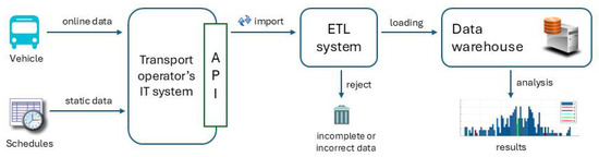
Figure 1.
Data collection scheme.
Accurate determination of bus routes requires the availability of public transport timetable data. The data source was the official timetables of the Public Transport Authority of the Capital City of Warsaw, available at [34]. Data is recorded in the general transit feed specification format [35]. It was used to obtain the following items for further analysis:
- The routes of the individual lines;
- The timetables of the individual lines;
- The coordinates of the stops for each line;
- The length and location of the inter-stop sections.
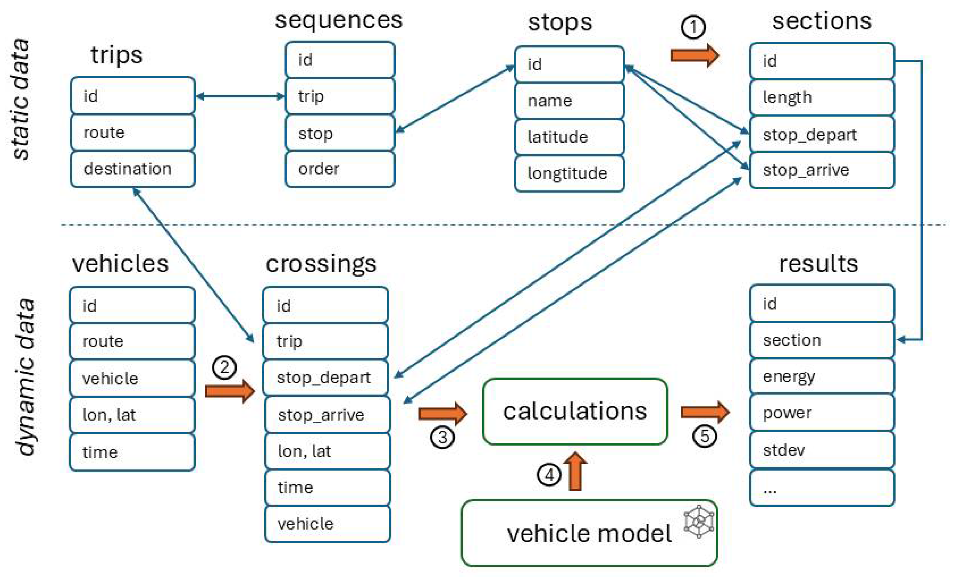
The following objects are stored in the data warehouse: each line’s public transport line trips, stops, and stop sequences. This is static data from timetables. A set of sections was created from these, with each element storing information about the line, the section length, and the start and end stops. The dynamic vehicle data is used for mathematical calculations utilising the vehicle model (Figure 2).
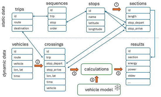
Figure 2.
Structures and data processing.
The analysis used bus trip data for Warsaw public transport from 2024. Three lines with different characteristics were selected to build the energy map (Table 2). The number of stops and the route length are given for both travel directions. The values before the slash refer to trips in one direction (“there”), and the values after the slash refer to trips in the opposite direction (“back”).
Table 2.
Summary of analysed routes.
2.2. Methods
Let be the set of all stops. Trip is the directed graph with vertices constituting a non-empty subset of stops , , connected using a set of directed edges . Edges represent possible connections between adjacent stops. Each edge in the graph that allows for making a trip from stop to will be called an inter-stop section (hereinafter: section). A section may be shared by multiple transport lines.
The extraction of sections is based on the data contained in the trips, sequences, and stops sets (Figure 2). A set of stops belonging to a set of trips is selected for each trip. It is then sorted cumulatively by order, based on the sequence of stops. The inter-stop sections are all pairs of stops to which equation applies. The extracted sections are saved to a set of sections (Figure 2, Step 1).
All trips relating to the route under analysis are selected from the set of vehicles. They are then subdivided into trips made by individual vehicles identified by registration number (vehicle column) and sorted by time (time column). This allows for obtaining all the trips a particular bus makes over the entire study period. Then, the acquired trips are linked to individual trips belonging to the line. Continuous trips along the route are then divided into so-called half-courses. The half-course starts at one of the trip’s end stops and ends at the other.
Figure 3 shows an example of a graph demonstrating a single bus’s progression of reaching stops per day for line number 112. The graph line indicates the order in which the bus stops are reached. Stops are numbered in order of location along the route from the start loop to the end loop. As can be seen, the bus makes a full or shortened trip.
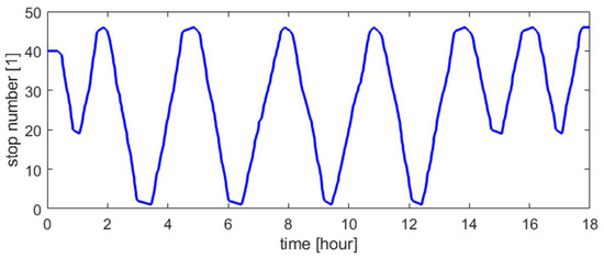
Figure 3.
Course of a single vehicle’s service trip per day.
The final step in acquiring service trips is to divide the half-course into individual sections. This yields a set of service trips for each section (Figure 2, Step 2). The operations are repeated for each communication line analysed (route column).
For clarity and ease of reference, all symbols used in the mathematical model are defined with their units in Table 3.
Table 3.
Definition of symbols.
The section trip is recorded as instantaneous measurements of the vehicle’s geographical location coordinates. The incremental increase in road between two measurements is calculated using the haversine formula, while speed is calculated as follows:
For building a vehicle model, we can use a variety of probabilistic, analytical, and empirical methods, computer simulations, machine learning methods, etc. [36,37,38,39]. Analytical methods focus on computer simulations or theoretical trips. Simulation methods analyse driving dynamics based on mathematical models expressed in differential equations. The calculations result in the achieved speed schedules. In contrast with the simulation approach, the theoretical trip involves solving a kinematic problem, i.e., determining traction forces from the required speed schedules [40].
The computational method presented in this paper refers to the theoretical trip method. According to the theoretical trip’s mathematical model
where is the traction force at the wheels, is the substitute vehicle weight taking into account the battery pack weight, is the speed waveform, and is the motion resistance force function approximated by a second-degree polynomial.
The incremental increase in the vehicle’s traction energy is calculated based on the power waveform, as:
where is the instantaneous traction power waveform, understood as the product of the mechanical drive force and the vehicle speed.
The mean power value in the given time is as follows:
Special cases of mean power are continuous power, calculated over the entire period under consideration, and 30 s power (calculated over time windows of 30 s). These powers are – 30 s peak power and – mean (continuous) power.
We will assume that the drive system consists of a mechanical reduction gear, an electrical machine, and an inverter. In modern converter drive systems, the electrical machine allows for bidirectional operation as a motor or generator. Electrical power can be expressed as:
where ia the power supply (electric) power, is the traction (mechanical at the wheels) power, is the power loss in the reduction gear, is the electric power loss in the machine inverter assembly, and is the machine operation type mark, where “+” is the engine operation and “−” is the generator operation.
The power loss in a reduction gear is usually described by a constant efficiency value:
where is the reduction gear’s energy efficiency (fixed parameter).
In contrast, the power loss in the traction machine inverter assembly depends on the operating point and the power for which the system is dimensioned:
where is the function of the traction machine power loss map as a function of the operating point, where is the torque and is the angular velocity. Index is the machine’s rated power.
Power losses are calculated using a universal model for describing the losses in the machine inverter assembly expressed in relative units, developed based on the actual power losses of 12 m bus drive systems [40]:
where is the polynomial fit weight, , .
The designated weights are shown in Table 4.
Table 4.
Loss function fit weights for the chosen system.
The formulae presented show that the machine’s power rating is of significant service importance as it contributes to electrical losses. In a properly serviced machine, it is related to the operating conditions, which is represented by the following relationship:
where is the maximum 30 s peak power, is the mean (continuous) power, and is the maximum allowable electrical machine overload factor.
3. Results
3.1. Results of the Analysis of Selected Route’s Section
Figure 4 shows the speed profile between the stops numbered 108510 (Bródno Underground 10) and 115002 (Suwalska Street 02). For convenience, unique internal stop identification numbers (stop IDs) from the public transport operator’s system are used for representation.
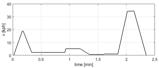
Figure 4.
Example of speed waveform for a selected section.
The speed probability distribution chart for all trips (4978) made on this section is shown in Figure 5. Speed classification was performed with a step of 5 kmph.
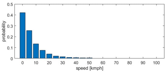
Figure 5.
Speed probability distribution for a selected section.
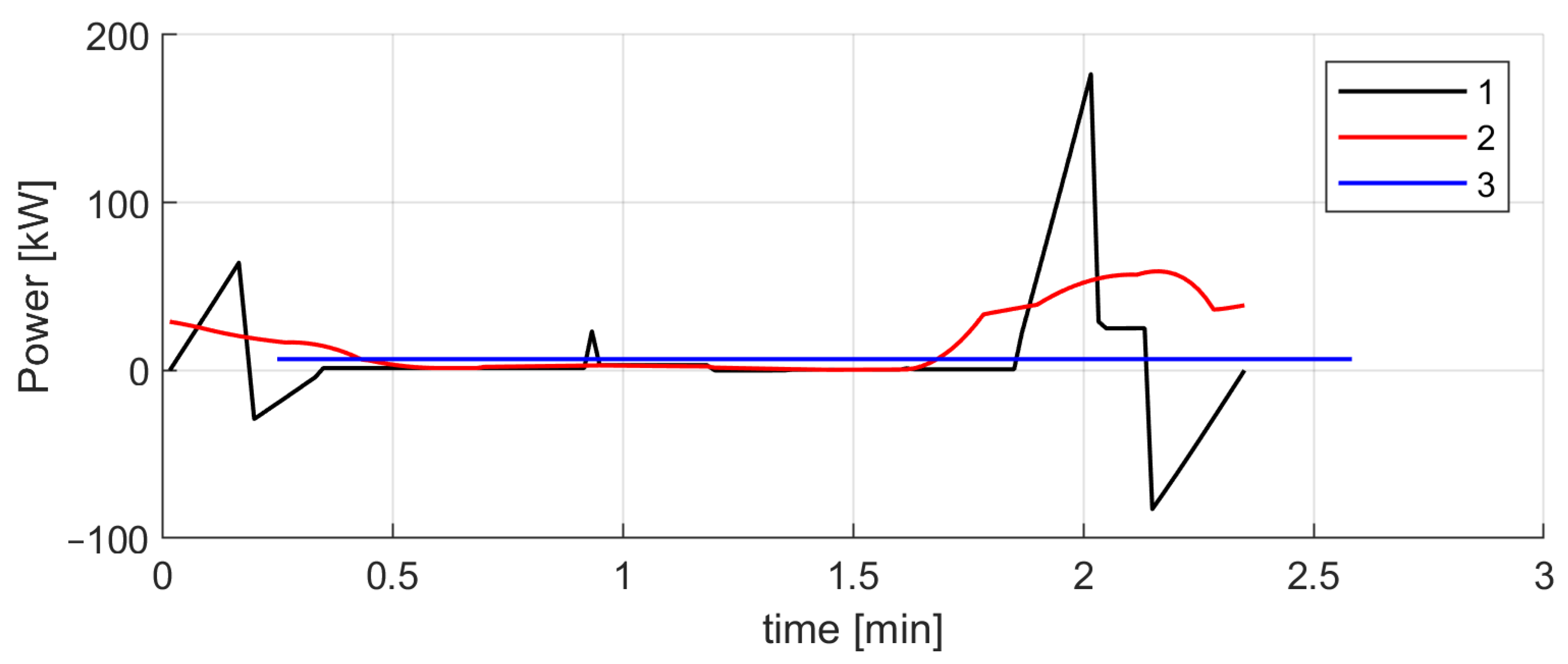
Figure 6 presents the following waveforms: instantaneous power , 30 s peak power , and mean power for the selected section. A high variability of the parameters characterising the power waveform can be observed. The maximum instantaneous power is 176 kW, the maximum 30 s peak power is 60 kW, and the mean power is equal to 10 kW.
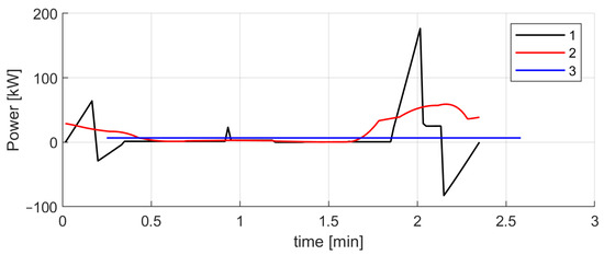
Figure 6.
Waveforms of instantaneous power (1), 30 s peak power (2), and mean power (3) for the selected section.
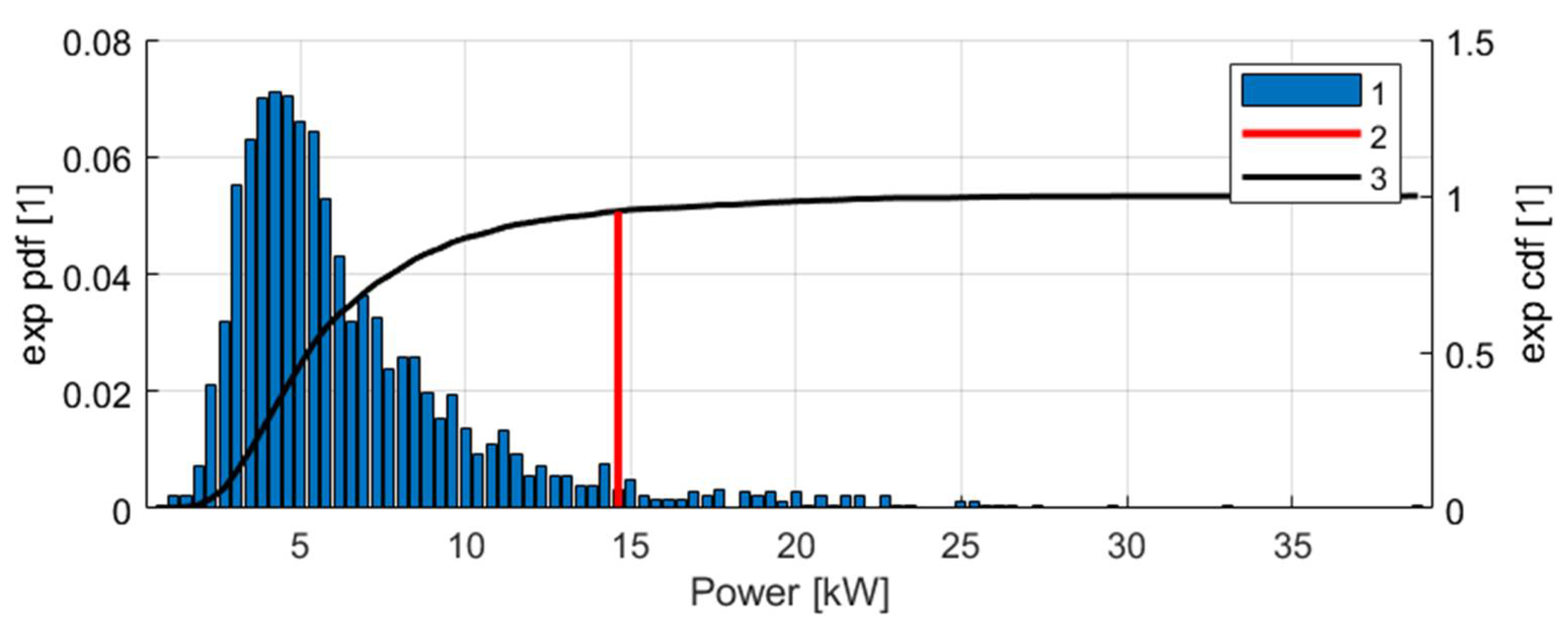
A new aspect of the research is the probabilistic evaluation of speed, energy, and power performance parameters using simple statistical methods such as classification, probability distribution, distribution function, and quantile. A chart of the probability distribution of the continuous drive power required to make the trips on the selected section is shown in Figure 7. The 95% quantile of continuous power is 15 kW.

Figure 7.
Experimental probability density function for the drive system’s continuous power on the selected section and its experimental cumulative distribution functions. The following components were designated: (1) density function, (2) distribution function, and (3) 95% quantile.
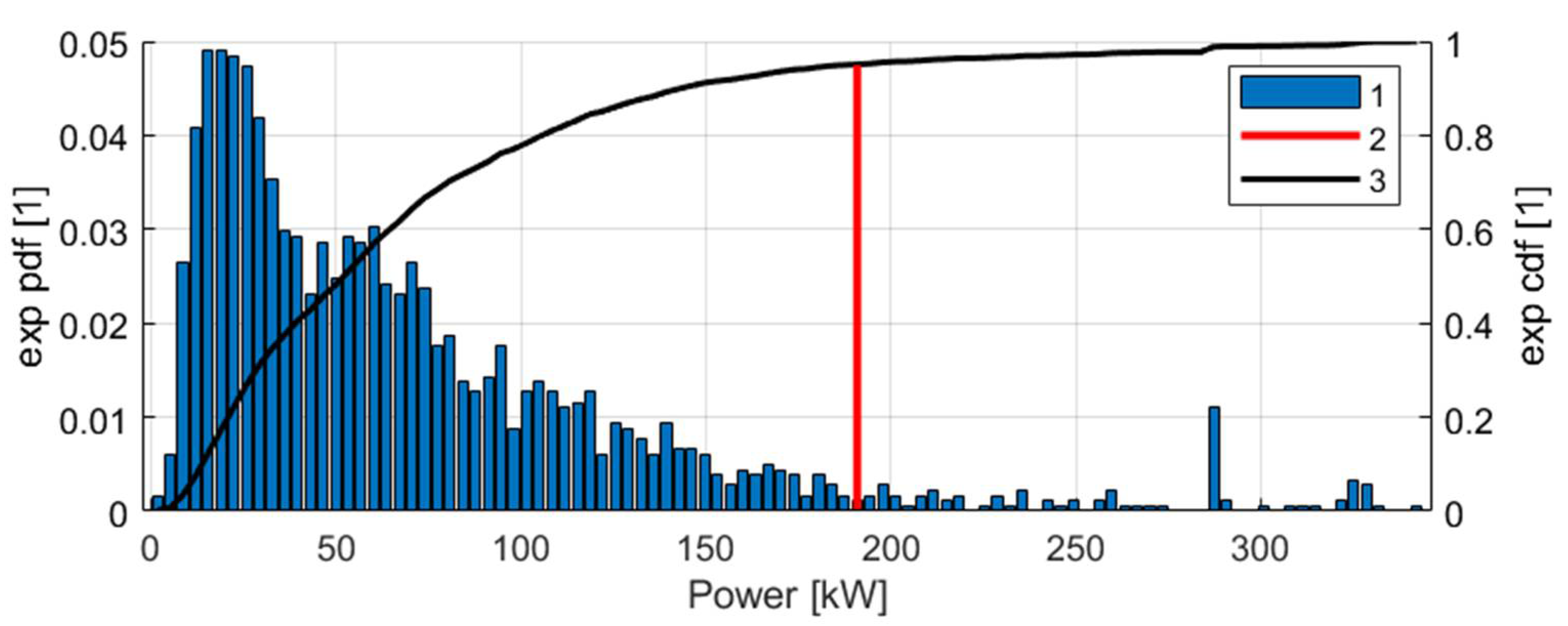
A chart of the probability distribution of the peak drive power required to make the trips on the selected section is shown in Figure 8. The 95% quantile of peak power is 191 kW.

Figure 8.
Experimental probability density function for the drive system’s peak power on the selected section and its experimental cumulative distribution functions. The following components were designated: (1) density function, (2) distribution function, and (3) 95% quantile.
It should be noted that the required continuous power is significantly smaller than the required peak power. The peak to continuous power ratio needed in this case is 190/15 = 12.6 kW. This wide variation in power is due to significant differences in how trips are made at different times of the day. During peak periods, pauses and stops during trips are long, resulting in low traffic speeds and power. At other times outside peak traffic, the instantaneous speeds and accelerations achieved may be higher, thus increasing the power demand.
3.2. Results of the Analysis of Service Trips
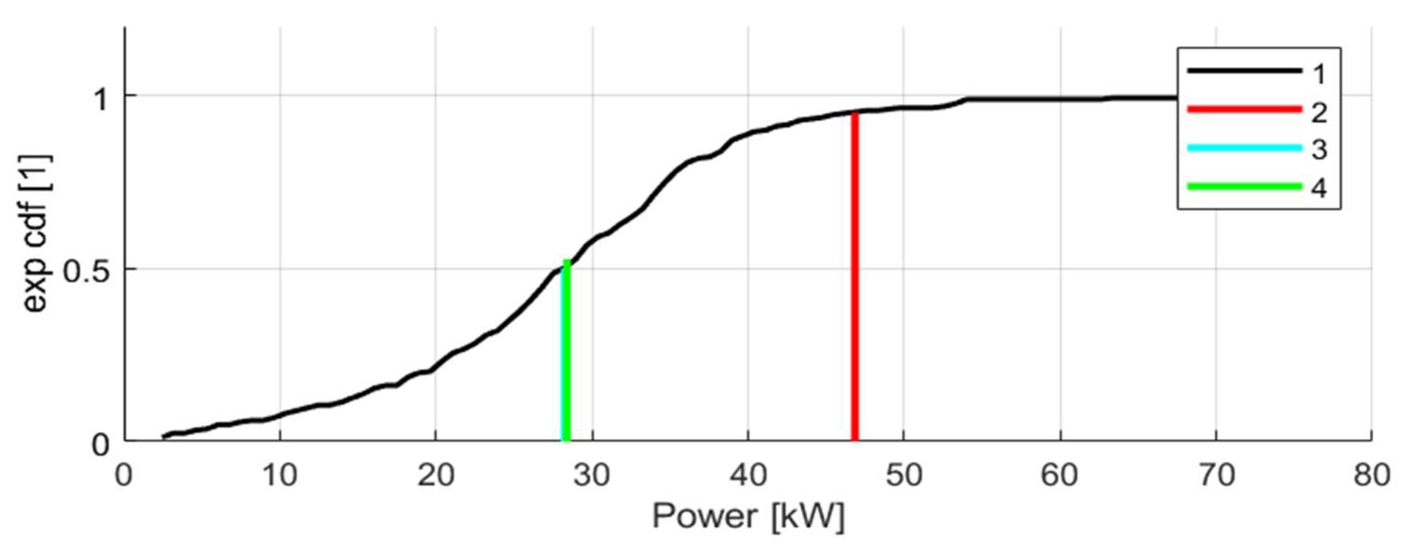
The analysis used 247 sections of the 3 bus routes: 112, 180, and 523. The total number of trips meeting the calculation conditions was 833,391. A chart of the probability distribution of the continuous power required on all sections is shown in Figure 9.
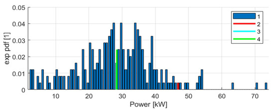
Figure 9.
Continuous power characteristics: distribution (1), 95% quantile (2), 50% quantile—median (3), mean value (4). The values are: 95% quantile—47 kW, median—28 kW, mean value—28 kW.
A chart of the continuous power distribution for all sections is shown in Figure 10.
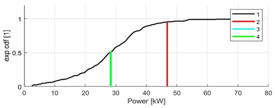
Figure 10.
Continuous power distribution for all sections.
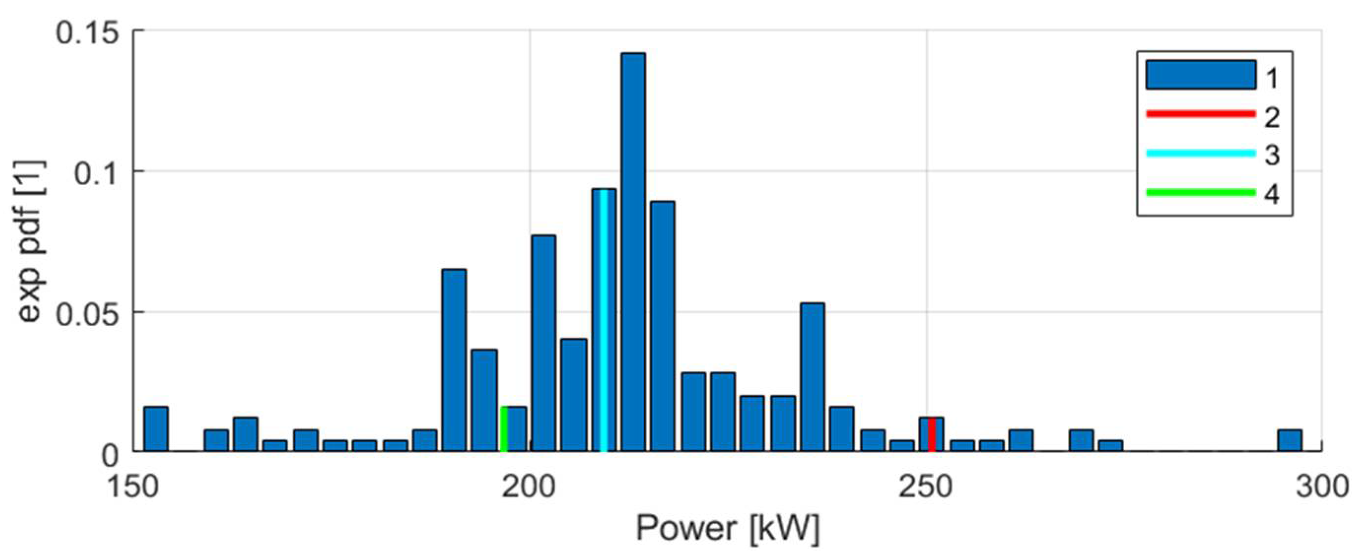
A chart of the probability distribution of the 30 s peak power is shown in Figure 11.
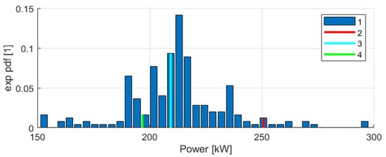
Figure 11.
Probability distribution of the 30 s peak power: distribution (1), 95% quantile (2), 50% quantile—median (3), mean value (4). The values are: 95% quantile—250 kW, median—209 kW, mean value—196 kW.
A chart of the peak power distribution is shown in Figure 12.

Figure 12.
Peak power distribution. The chart shows distribution (1), 95% quantile (2), 50% quantile—median (3), mean value (4). The values are the same as above.
Based on the analysis of all trips from all sections, the conclusions are as follows: The required 30 s peak power is 250 kW, while the continuous power is 47 kW. Peak power is approx. 5 times greater than the continuous power.
3.3. Estimated Incremental Increase in Electricity
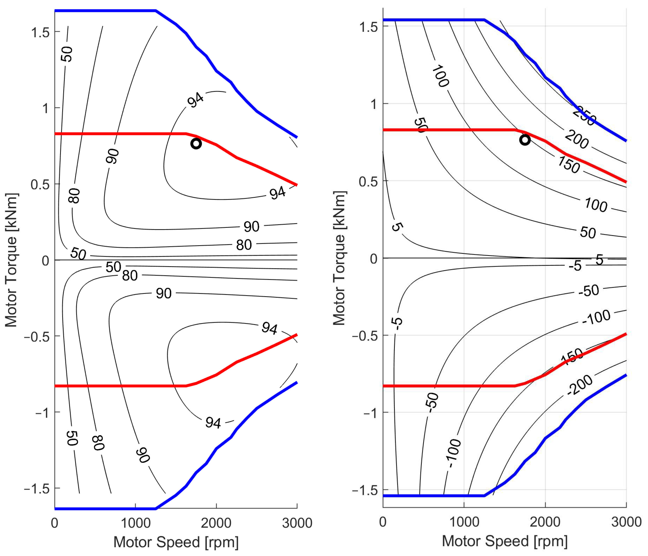
The analysis results of the operating power waveforms are characterised by the 95% quantiles of the continuous and peak power’s probability distribution, which amount to 50 and 250 kW, respectively. In practice, due to the design limitation of the electrical machines’ overload capacity, these requirements will be met by traction machines whose maximum 30 s power is not less than the service peak power of 250 kW, and whose rated continuous power exceeds 140 kW.
Figure 13 shows the efficiency and power maps of the drive system (machine inverter) obtained with these parameters using the loss model shown above.
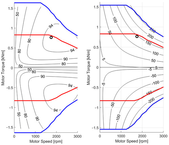
Figure 13.
The drive system’s efficiency map (left) and power map (right).
The method used to analyse the service traffic conditions and the method used to select the drive system show that a system with the designated parameters can operate correctly under traffic conditions covering 95% of the conditions observed in service to date. However, due to the design limitation of the electrical machines’ overload factor, the machine’s 140 kW rated power far exceeds the 50 kW of the 95% quantile of mean power. This means the drive system will be loaded under most operating conditions with less than the rated power. Under these conditions, the drive system’s power conversion efficiencies can be significantly lower than the nominal values.
3.4. Energy Demand Map
The calculations of the energy consumption of the electric vehicle’s battery required to cover the different sections of the selected routes were recorded in a table. An extract of this data is presented in Table 5.
Table 5.
Result of energy distribution calculations for all sections (extract).
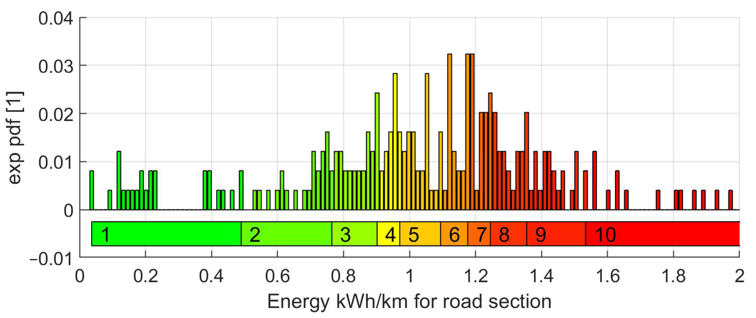
The probability distribution of the electricity’s incremental increase (converted per 100 km) required to cover a road section is shown in Figure 14.
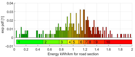
Figure 14.
Probability distribution of the energy incremental increase per section. The colour palette is presented in Table 6.
The energy distribution was divided into 10 classes of equal probability. Class boundaries are quantiles of the order of . This division ensures the number of sections in the class sets is equal. The class boundaries are summarised in Table 6.
Table 6.
The class boundaries for energy (EE, kWh/km) and peak power (P, kW).
The probability distribution of the 30 s peak power demand required to cover the road sections is shown in Figure 15. As with the energy distribution, the power distribution was divided into 10 disjoint classes according to the principle of equal probability.
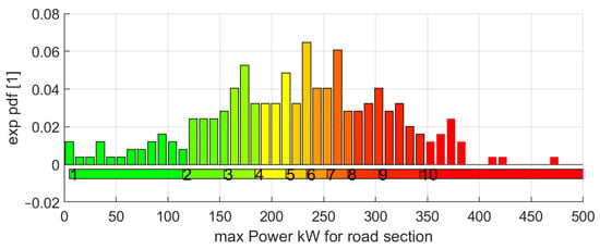
Figure 15.
Probability distribution of the 30 s peak power on the section. The colour palette is presented in Table 6.
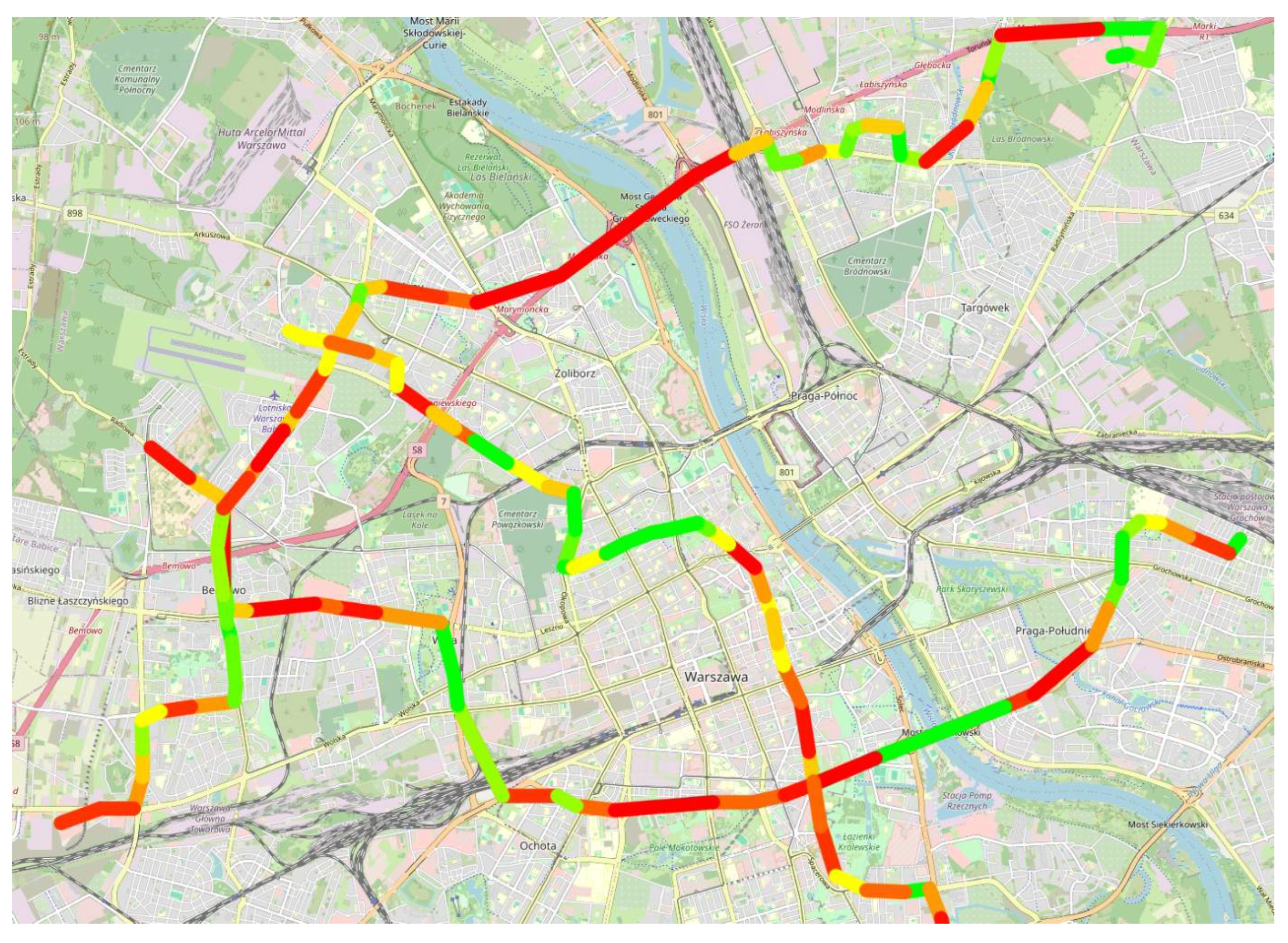
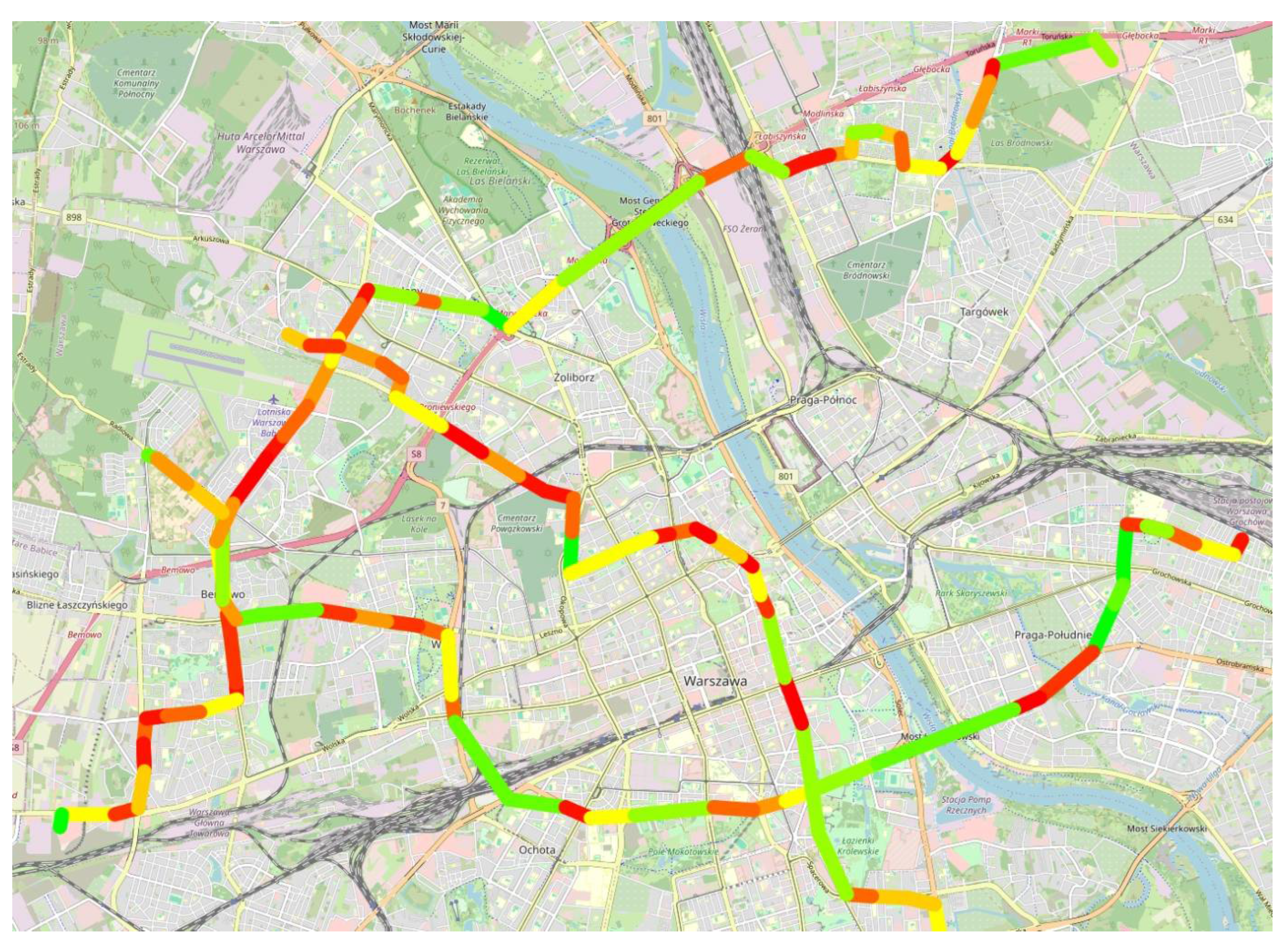
The OpenStreetMap platform was used to visualise the results of the calculations in the form of a map [41]. Each record in Table 4 represents a route section between two stops. A polyline connected the adjacent stops. The colour of the line connecting the sections is a gradient from green (minimum values) to red (maximum values). The map generation script was written in Python 3.12 using the Folium library, which provides support for OpenStreetMap.
Figure 16 shows a map illustrating the incremental increase in energy consumption for trips “there”, while Figure 17 shows the incremental increase for trips “back”. Separate maps for trips “there” and “back” have been created to increase the maps’ readability.
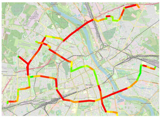
Figure 16.
Energy map for “there” trips. The colour palette is presented in Table 6.
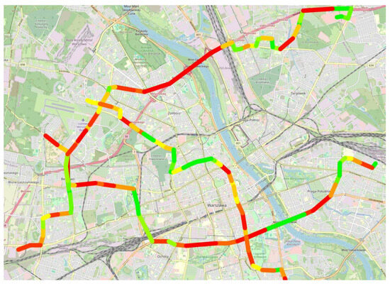
Figure 17.
Energy map for “back” trips. The colour palette is presented in Table 6.
Figure 18 shows a map illustrating the 30 s peak power for trips “there”, while Figure 19 shows the peak power for trips “back”.

Figure 18.
The 30 s peak power map for “there” trips. The colour palette is presented in Table 6.
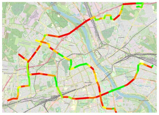
Figure 19.
The 30 s peak power map for “back” trips. The colour palette is presented in Table 6.
4. Discussion
To our knowledge, the representation of energy consumption and peak power demand on detailed maps of road sections has not been encountered in the literature so far.
While classical “theoretical trip” models and kinematic equations have long been used to approximate vehicle energy requirements, our work combines these models with two years of real-world measurement data from all Warsaw bus lines. This fusion of empirical data and established theory allows us to capture the real variability of urban operations.
A key finding is the large gap between continuous power demand and 30 s peak power; the 95th percentile of peak power is roughly five times greater than that of continuous demand. This discrepancy reflects the frequent intense acceleration events that transiently overload the drive system, especially in stop-and-go traffic. Electric motors can sustain short-term overloads. Designing motors for these peaks forces the selection of larger continuous-rated motors. When operating under insufficient load, they operate with less energy efficiency.
Also, the energy maps become decision-support tools. Operators can tailor service in several ways by highlighting “hot spots” with consistently high energy or peak power demands. Timetable adjustments or driver training can mitigate energy-intensive driving behaviours. Targeted infrastructure upgrades, such as dedicated bus lanes or optimised traffic signals, can smooth traffic flow. And planners designing new or modified routes can choose lower-demand route segments to minimise total energy use and ensure compatibility with available vehicle specifications.
In our modelling, we account for passenger load by assuming a representative operating mass of 16,600 kg (12,000 kg empty plus 4000 kg payload at ~50 passengers), applying a 1.05 rotational mass coefficient. This figure aligns with real-world electric bus specifications (e.g., Solaris Urbino 12 Electric: 10,900 kg unladen, 18,000 kg GVW). In electric buses, the heavy battery pack dominates total mass, so variations in passenger count have a proportionally smaller effect on acceleration energy than in diesel buses.
Although our results derive from only three representative lines in Warsaw, the methodology is fully scalable and generalisable. Extending this approach to other cities requires access to similarly detailed operator data, vehicle and loss-map parameter recalibration, and calculation power for processing large datasets. Under these conditions, probabilistic independence assumptions (e.g., via Kruskal–Wallis tests) ensure that significant differences between sections can be properly identified.
Future work will build on this foundation in several directions: optimising charging station siting and power ratings under budgetary constraints; integrating probabilistic energy profiles with battery aging and life-cycle cost models; enriching our maps with meteorological variables (temperature, precipitation) to produce weather-sensitive demand profiles; and exploring how network design choices (route length, stop frequency, service intervals) influence energy use. We also plan to leverage the same dataset for service reliability studies using clustering and machine-learning techniques (e.g., LSTM networks) to predict arrival delays and enhance timetable robustness.
Finally, by aggregating analogous maps from multiple urban areas, we envision a “city-type profiling” approach, i.e., clustering cities into categories (large metropolises, mid-sized cities, smaller towns) based on their characteristic energy demand distributions. With temporal segmentation (day of week, time of day) and weather factors, such profiles would enable rapid energy requirement assessments in unmapped cities with similar operational characteristics.
In sum, this paper demonstrates a flexible data-driven approach that advances the theoretical modelling of electric bus energy demand and delivers usable energy maps for strategic planning in sustainable urban mobility.
5. Conclusions
In this paper, we have presented a data-driven probabilistic methodology for mapping electric buses’ energy consumption and 30 s peak power demand on a section-by-section basis. The method rests on the following three core assumptions:
- Availability of two years of high-resolution operational data from onboard bus recorders, accessed via the transport operator’s IT system;
- Use of classical “theoretical trip” models (kinematic equations) to derive instantaneous traction forces and power waveforms from recorded speed profiles;
- Application of detailed inverter motor loss maps to convert mechanical traction power into electrical energy demand.
Key findings include the following:
- A large discrepancy between continuous and peak power demands, with the 95th percentile of peak power exceeding that of continuous power by a factor of approximately five;
- High variability of energy use and power requirements across different route sections, underscoring the importance of section-level analysis rather than aggregated averages.
Our work offers a set of urban energy and peak power demand maps that can immediately support the following:
- Strategic charger placement and sizing along routes, by identifying “hot spots” of high energy or power demand;
- Rational dimensioning of battery capacity and traction motor power, ensuring reliable operation under real-world conditions;
- Route planning and verification, by providing pre-computed energy estimates for existing and newly configured routes.
As future research directions, we recommend the following:
- Integration of our maps with charger location models to optimise both siting and power ratings under budgetary and operational constraints (charger network optimisation);
- Combine our probabilistic energy profiles with battery ageing models to predict life-cycle costs and replacement schedules (advanced battery analysis);
- Incorporation of ambient temperature, precipitation (rain/snow), and other weather variables to enrich our profiling, enabling energy demand maps that vary by weather conditions (integration of meteorological data);
- Exploration of how network parameters (route length, stop frequency, service intervals) impact energy use, in collaboration with established bus network design heuristics (network design implications);
- Leveraging the same dataset to build statistical and machine-learning models (e.g., Kruskal–Wallis clustering, post hoc tests, and future LSTM networks) that predict bus arrival delays and inform timetable resilience (delay prediction and punctuality).
While the methodology is fully portable to any city with comparable operational data, the specific maps presented here are tailored to Warsaw’s flat topography, traffic patterns, and service characteristics. Extending these maps to other cities requires the following:
- Access to similarly detailed operator data;
- Recalibration of vehicle and loss model parameters to match local bus specifications and driving conditions;
- Management of massive datasets (tens to hundreds of millions of records), which, while uncountable in practice, lend themselves to probabilistic independence assumptions—almost any section-level difference will be statistically significant under tests like Kruskal–Wallis with post hoc analysis.
We propose clustering and city-type profiling as a probabilistic method to solve this problem. By aggregating similarly derived maps from multiple cities, we envision creating city-type profiles classifying urban areas into clusters (e.g., large metropolises, mid-sized cities, smaller towns) based on their characteristic energy demand distributions. Such profiles, combined with temporal segmentation (day of week, time of day, weather), would support rapid assessment of energy requirements in unmapped cities that share known profiles.
In summary, this work is a case study demonstrating the power and flexibility of a data-driven probabilistic framework for electric bus energy mapping. We invite further research to expand, adapt, and integrate these maps into comprehensive planning and operational systems for sustainable urban mobility.
Author Contributions
Conceptualisation, A.C. and M.K.; methodology, M.K.; software, A.C.; validation, M.K.; formal analysis, A.C. and M.K.; investigation, M.K.; resources, A.C.; data curation, A.C.; writing—original draft preparation, A.C. and M.K.; writing—review and editing, A.C.; visualisation, M.K.; supervision, M.K.; project administration, A.C.; funding acquisition, A.C. All authors have read and agreed to the published version of the manuscript.
Funding
This paper was co-financed under the research grant of the Warsaw University of Technology supporting the scientific activity in the discipline of Civil Engineering, Geodesy, and Transport, grant number 1/ILGiT/2024.
Data Availability Statement
The raw data supporting the conclusions of this article will be made available by the authors on request.
Conflicts of Interest
The authors declare no conflicts of interest.
References
- Indumathi, R. Electric Vehicles and Environmental Sustainability. ANWESH Int. J. Manag. Inf. Technol. 2020, 5, 5. [Google Scholar]
- Mo, T.; Li, Y.; Lau, K.; Poon, C.K.; Wu, Y.; Luo, Y. Trends and Emerging Technologies for the Development of Electric Vehicles. Energies 2022, 15, 6271. [Google Scholar] [CrossRef]
- Majumder, S.; De, K.; Kumar, P. Zero Emission Transportation System. In Proceedings of the 2016 IEEE International Conference on Power Electronics, Drives and Energy Systems (PEDES), Trivandrum, India, 14–17 December 2016; IEEE: Piscataway, NJ, USA, 2016; pp. 1–6. [Google Scholar]
- Brdulak, A.; Chaberek, G.; Jagodziński, J. Development Forecasts for the Zero-Emission Bus Fleet in Servicing Public Transport in Chosen EU Member Countries. Energies 2020, 13, 4239. [Google Scholar] [CrossRef]
- Stec, S. Assessment of the Economic Efficiency of the Operation of Low-Emission and Zero-Emission Vehicles in Public Transport in the Countries of the Visegrad Group. Energies 2021, 14, 7706. [Google Scholar] [CrossRef]
- Rizza, V.; Torre, M.; Tratzi, P.; Fazzini, P.; Tomassetti, L.; Cozza, V.; Naso, F.; Marcozzi, D.; Petracchini, F. Effects of Deployment of Electric Vehicles on Air Quality in the Urban Area of Turin (Italy). J. Environ. Manag. 2021, 297, 113416. [Google Scholar] [CrossRef]
- Marotta, A.; Lodi, C.; Julea, A.; Gómez Vilchez, J.J. European Governments’ Electromobility Plans: An Assessment with a Focus on Infrastructure Targets and Vehicle Estimates until 2030. Energy Effic. 2023, 16, 92. [Google Scholar] [CrossRef]
- Electromobility and Alternative Fuels Act. Available online: https://sip.lex.pl/akty-prawne/dzu-dziennik-ustaw/elektromobilnosc-i-paliwa-alternatywne-18683445 (accessed on 13 April 2024).
- Polish Automotive Industry Association 2024 Year of Stagnation in Electric Car Market, Infrastructure on the Upside. Available online: https://www.pzpm.org.pl/pl/Elektromobilnosc/Licznik-Elektromobilnosci/Rok-2024/Grudzien-2024 (accessed on 15 April 2025).
- Zeng, Z.; Wang, S.; Qu, X. On the Role of Battery Degradation in En-Route Charge Scheduling for an Electric Bus System. Transp. Res. Part E Logist. Transp. Rev. 2022, 161, 102727. [Google Scholar] [CrossRef]
- Tepe, B.; Jablonski, S.; Hesse, H.; Jossen, A. Lithium-Ion Battery Utilization in Various Modes of e-Transportation. eTransportation 2023, 18, 100274. [Google Scholar] [CrossRef]
- Perumal, S.S.G.; Lusby, R.M.; Larsen, J. Electric Bus Planning & Scheduling: A Review of Related Problems and Methodologies. Eur. J. Oper. Res. 2022, 301, 395–413. [Google Scholar] [CrossRef]
- Avenali, A.; Catalano, G.; Giagnorio, M.; Matteucci, G. Factors Influencing the Adoption of Zero-Emission Buses: A Review-Based Framework. Renew. Sustain. Energy Rev. 2024, 197, 114388. [Google Scholar] [CrossRef]
- Brozovsky, J.; Gustavsen, A.; Gaitani, N. Zero Emission Neighbourhoods and Positive Energy Districts—A State-of-the-Art Review. Sustain. Cities Soc. 2021, 72, 103013. [Google Scholar] [CrossRef]
- Tsoi, K.H.; Loo, B.P.Y.; Li, X.; Zhang, K. The Co-Benefits of Electric Mobility in Reducing Traffic Noise and Chemical Air Pollution: Insights from a Transit-Oriented City. Environ. Int. 2023, 178, 108116. [Google Scholar] [CrossRef] [PubMed]
- Zhang, J.; Zhao, A.; Tang, C. Integrated Optimization of Mixed Bus Fleet Replacement and Scheduling with Emission and Budget Constraints. Preprint 2025. [Google Scholar]
- Gairola, P.; Nezamuddin, N. Determining Battery and Fast Charger Configurations to Maximize E-Mileage of Electric Buses under Budget. J. Transp. Eng. Part A Syst. 2022, 148, 04022100. [Google Scholar] [CrossRef]
- Wenz, K.-P.; Serrano-Guerrero, X.; Barragán-Escandón, A.; González, L.G.; Clairand, J.-M. Route Prioritization of Urban Public Transportation from Conventional to Electric Buses: A New Methodology and a Study of Case in an Intermediate City of Ecuador. Renew. Sustain. Energy Rev. 2021, 148, 111215. [Google Scholar] [CrossRef]
- Czerepicki, A.; Choromański, W.; Kozłowski, M.; Kazinski, A. Analysis of the Problem of Electric Buses Charging in Urban Transport. Sci. Tech. 2020, 19, 349–355. [Google Scholar] [CrossRef]
- Zhou, Y.; Meng, Q.; Ong, G.P. Electric Bus Charging Scheduling for a Single Public Transport Route Considering Nonlinear Charging Profile and Battery Degradation Effect. Transp. Res. Part B Methodol. 2022, 159, 49–75. [Google Scholar] [CrossRef]
- Olsen, N.; Kliewer, N. Location Planning of Charging Stations for Electric Buses in Public Transport Considering Vehicle Scheduling: A Variable Neighborhood Search Based Approach. Appl. Sci. 2022, 12, 3855. [Google Scholar] [CrossRef]
- Szilassy, P.Á.; Földes, D. Consumption Estimation Method for Battery-Electric Buses Using General Line Characteristics and Temperature. Energy 2022, 261, 125080. [Google Scholar] [CrossRef]
- Zhang, X.; Nie, S.; He, M.; Wang, J. Charging System Analysis, Energy Consumption, and Carbon Dioxide Emissions of Battery Electric Buses in Beijing. Case Stud. Therm. Eng. 2021, 26, 101197. [Google Scholar] [CrossRef]
- Li, P.; Jiang, M.; Zhang, Y.; Zhang, Y. Cooperative Optimization of Bus Service and Charging Schedules for a Fast-Charging Battery Electric Bus Network. IEEE Trans. Intell. Transp. Syst. 2023, 24, 5362–5375. [Google Scholar] [CrossRef]
- Behnia, F.; Schuelke-Leech, B.-A.; Mirhassani, M. Optimizing Sustainable Urban Mobility: A Comprehensive Review of Electric Bus Scheduling Strategies and Future Directions. Sustain. Cities Soc. 2024, 108, 105497. [Google Scholar] [CrossRef]
- Weiss, M.; Winbush, T.; Newman, A.; Helmers, E. Energy Consumption of Electric Vehicles in Europe. Sustainability 2024, 16, 7529. [Google Scholar] [CrossRef]
- Lee, G.; Song, J.; Lim, Y.; Park, S. Energy Consumption Evaluation of Passenger Electric Vehicle Based on Ambient Temperature under Real-World Driving Conditions. Energy Convers. Manag. 2024, 306, 118289. [Google Scholar] [CrossRef]
- Zhang, J.; Wang, Z.; Liu, P.; Zhang, Z. Energy Consumption Analysis and Prediction of Electric Vehicles Based on Real-World Driving Data. Appl. Energy 2020, 275, 115408. [Google Scholar] [CrossRef]
- Jonas, T.; Wilde, T.; Hunter, C.D.; Macht, G.A. The Impact of Road Types on the Energy Consumption of Electric Vehicles. J. Adv. Transp. 2022, 2022, 1436385. [Google Scholar] [CrossRef]
- Ou, X.; Zhang, X.; Chang, S. Alternative Fuel Buses Currently in Use in China: Life-Cycle Fossil Energy Use, GHG Emissions and Policy Recommendations. Energy Policy 2010, 38, 406–418. [Google Scholar] [CrossRef]
- Skrúcaný, T.; Kendra, M.; Stopka, O.; Milojević, S.; Figlus, T.; Csiszár, C. Impact of the Electric Mobility Implementation on the Greenhouse Gases Production in Central European Countries. Sustainability 2019, 11, 4948. [Google Scholar] [CrossRef]
- Borghetti, F.; Carra, M.; Besson, C.; Matarrese, E.; Maja, R.; Barabino, B. Evaluating Alternative Fuels for a Bus Fleet: An Italian Case. Transp. Policy 2024, 154, 1–15. [Google Scholar] [CrossRef]
- Warsaw City Administration. Open Data. Available online: https://api.um.warszawa.pl/# (accessed on 13 April 2024).
- Warsaw Public Transport Timetables. Available online: https://www.ztm.waw.pl/pliki-do-pobrania/dane-rozkladowe/ (accessed on 16 April 2025).
- General Transit Feed Specification. Available online: https://gtfs.org/documentation/overview/ (accessed on 16 April 2025).
- Basma, H.; Mansour, C.; Haddad, M.; Nemer, M.; Stabat, P. Energy Consumption and Battery Sizing for Different Types of Electric Bus Service. Energy 2022, 239, 122454. [Google Scholar] [CrossRef]
- Chen, Y.; Zhang, Y.; Sun, R. Data-Driven Estimation of Energy Consumption for Electric Bus under Real-World Driving Conditions. Transp. Res. Part D Transp. Environ. 2021, 98, 102969. [Google Scholar] [CrossRef]
- Lim, L.K.; Muis, Z.A.; Ho, W.S.; Hashim, H.; Bong, C.P.C. Review of the Energy Forecasting and Scheduling Model for Electric Buses. Energy 2023, 263, 125773. [Google Scholar] [CrossRef]
- Fiori, C.; Montanino, M.; Nielsen, S.; Seredynski, M.; Viti, F. Microscopic Energy Consumption Modelling of Electric Buses: Model Development, Calibration, and Validation. Transp. Res. Part D Transp. Environ. 2021, 98, 102978. [Google Scholar] [CrossRef]
- Kozłowski, M.; Czerepicki, A. Quick Electrical Drive Selection Method for Bus Retrofitting. Sustainability 2023, 15, 10484. [Google Scholar] [CrossRef]
- OpenStreet Map. Available online: https://www.openstreetmap.org/ (accessed on 10 June 2024).


Disclaimer/Publisher’s Note: The statements, opinions and data contained in all publications are solely those of the individual author(s) and contributor(s) and not of MDPI and/or the editor(s). MDPI and/or the editor(s) disclaim responsibility for any injury to people or property resulting from any ideas, methods, instructions or products referred to in the content. |
© 2025 by the authors. Licensee MDPI, Basel, Switzerland. This article is an open access article distributed under the terms and conditions of the Creative Commons Attribution (CC BY) license (https://creativecommons.org/licenses/by/4.0/).