Optimal Allocation of Shared Energy Storage in Low-Carbon Parks Taking into Account the Uncertainty of Photovoltaic Output and Electric Vehicle Charging

Abstract

The growing integration of renewable energy and electric vehicle loads in parks has intensified the intermittency of photovoltaic (PV) output and demand-side uncertainty, complicating energy storage system design and operation. Meanwhile, under carbon neutrality goals, the energy system must balance economic efficiency with emission reductions, raising the bar for storage planning. To address these challenges, this study proposes a two-stage robust optimization method for shared energy storage configuration in a park-level integrated PV–storage–charging system (PV-SESS-CS). The method considers the uncertainties of PV and electric vehicle (EV) loads and incorporates carbon emission reduction benefits. First, a configuration model for shared energy storage that accounts for carbon emission reduction is established. Then, a two-stage robust optimization model is developed to characterize the uncertainties of PV output and EV charging demand. Typical PV output scenarios are generated using Latin Hypercube Sampling, and representative PV profiles are extracted via K-means clustering. For EV charging loads, uncertainty scenarios are generated using Monte Carlo Sampling. Finally, simulations are conducted based on real-world industrial park data. The results demonstrate that the proposed method can effectively mitigate the negative impact of source-load fluctuations, significantly reduce operating costs, and enhance carbon emission reductions. This study provides strong methodological support for optimal energy storage planning and low-carbon operation in park-level PV-SESS-CS.

1. Introduction

With the continuous growth of the global economy, the demand for electricity in industrial parks is rising, and the wide application of electric vehicles (EVs) has further aggravated the demand for charging energy in industrial parks [1]. In this context, the construction of the charging station (CS) integrated with a photovoltaic and shared energy storage system (PV-SESS-CS) in the park has become an efficient solution. By integrating stable industrial loads into PV-SESS-CS, a deeply coupled and integrated operation pattern of ‘generation–load–storage–charging’ can be established. Given that most industrial parks in China adopt a unified electricity account and centralized settlement mechanism, all users typically share a common grid connection point and a single electricity account, with all electricity transactions settled collectively by the park operator. As a result, the shared energy storage system (SESS) generally lacks the metering, access rights, and pricing mechanisms required to participate in electricity markets and is primarily used for internal load balancing and photovoltaic (PV) output optimization within the park. In the planning and construction of SESS, how to rationally allocate energy storage capacity has become a key issue. Reasonable energy storage capacity configuration can not only optimize the operating efficiency of the power system but also provide necessary power support when the photovoltaic output is insufficient or the charging demand of electric vehicles is at its peak [2]. In addition, carbon emission reduction has become an important factor in the development of industrial parks. Considering carbon reduction benefits in the energy storage configuration process not only helps reduce greenhouse gas emissions but also brings policy support and economic incentives to the park, thereby enhancing its capacity for sustainable development [3].

In terms of energy optimization in the park, the current research mainly focuses on the planning and design of multi-energy and multi-network integration. Reference [4] proposed an energy system integration model for industrial parks considering multi-network integration and introduced a step-by-step carbon trading mechanism into the model to reduce carbon emissions and optimize the scheduling of carbon trading models. Aiming at the problems of a low-energy utilization rate, unreasonable energy structure and large peak-valley power differences in industrial parks, reference [5] proposed a regional integrated energy system management strategy based on energy cascade utilization, which realized the high efficiency and stability of the system. The integration of PV and buildings provides a flexible form of energy use for the park. Reference [6] summarizes the technology of combining the energy storage system with building-integrated photovoltaics (BIPVs); analyzes the current situation, research, development, application, obstacles and challenges of BIPV with the energy storage system; and proposes that the integration of BIPV and energy storage can improve the reliability of energy utilization in the park. The above literature provides useful help for the energy application of the park, but it is difficult to cope with the increasing demand for EV charging, and it is difficult to ensure the low-carbon energy consumption of the park.

At the same time, the energy demand and timing of the park, including PV, energy storage and EV charging piles, are complex. At present, most of the research is on the integrated CS or energy hub including PV and energy storage. Reference [7] proposed a two-stage robust planning operation collaborative optimization method considering renewable energy uncertainty and multi-load demand and studied the scale determination problem and accurate economic model of energy storage system, but the study lacked consideration of carbon emission reductions. A unified planning model of distributed generation and EV CSs considering multiple uncertainties and battery degradation is established. Reference [8] proposed a unified planning model of distributed generation and EV CSs considering multiple uncertainties and battery degradation and used the Latin Hypercube Sampling (LHS) method to generate multiple scenarios to describe the uncertainty of renewable energy and load demand. In reference [9], a new energy collaboration framework integrating community energy storage and a PV CS cluster is proposed, which aims to balance grid load, improve energy utilization, enhance power system stability, and provide guidance for the planning of PV-SESS-CS in the park. However, the above research rarely covered the coordinated scheduling of PV-SESS-CS in the park. The configuration method of shared energy storage considering the fluctuations in PV and charging in the park needs to be further studied.

The optimal allocation of shared energy storage in low-carbon parks considering the uncertainty of PV output and EV charging involves the randomness of PV and charging, which adds a new burden to the planning of shared energy storage in parks, and it is necessary to study effective solution algorithms. In reference [10], a multi-objective robust optimization strategy is proposed to deal with the uncertainties caused by distributed generation, the diversity of demand response and the flexibility of topology. By constructing an uncertainty set for predicting the maximum output of PV power generation, the optimization results under different uncertainty sets are obtained. Reference [11] investigates the lifecycle coordinated planning of Multi-Energy Ship Microgrids and proposes a two-stage robust optimization framework that accounts for thermal inertia and ship navigation uncertainties, such as wave and wind disturbances, thereby enhancing system safety and economic efficiency during maritime operations. Reference [12] addresses the planning of Networked Hydrogen-Electrical Microgrids and highlights the importance of the demand-inducing effect, where hydrogen refueling demand is influenced by infrastructure investment. To capture this endogeneity, a trilevel stochastic-robust optimization model is developed using decision-dependent uncertainty, providing a flexible and rigorous framework for modeling such interdependencies. Specifically, the aforementioned studies focus on planning problems involving various complex energy resources and operational characteristics, such as diesel generators, gas turbines, hydrogen storage systems, hydrogen refueling stations, wind/PV renewable generation, propulsion loads, and the thermal inertia of ships. Their primary objectives are often long-term investment and operation planning under multi-source coupling or maritime energy supply scenarios.

Based on the historical data-driven search algorithm, reference [13] proposed a PV and energy storage capacity allocation method for the integrated PV and energy storage CS and obtained the configuration capacity of energy storage with the goal of maximizing economic benefits. However, the existing research is still insufficient in considering the multi-energy coupling characteristics and complex load fluctuation in the industrial park, especially in the flexibility and economic guarantee of energy storage configuration.

In summary, in view of the shortcomings of existing research on the optimal allocation of shared energy storage capacity in park-level PV-SESS-CS systems, this study proposes an optimal allocation method for shared energy storage in low-carbon parks, considering the uncertainties of PV output and EV charging. The main contributions of this study are summarized as follows:

(1)

A shared energy storage configuration model is developed that incorporates carbon emission reduction benefits via the China Certified Emission Reduction (CCER) market mechanism, offering a policy-aligned pathway for low-carbon park operations.

(2)

A two-stage robust optimization model is proposed to address the dual uncertainties of PV output and EV charging demand and is solved using a column-and-constraint generation (C&CG) algorithm to ensure solution feasibility and robustness.

(3)

LHS and K-means clustering are employed to generate representative PV output scenarios, while an EV charging model combined with Monte Carlo Sampling (MCS) is used to construct load demand scenarios, ensuring the accurate and efficient characterization of system uncertainties.

(4)

Simulation studies based on a typical industrial park are carried out to verify the effectiveness of the proposed method in improving economic performance and carbon reduction, demonstrating its practical applicability in shared energy storage planning under park-level PV-SESS-CS systems.

The structure of this paper is as follows: Section 2 introduces the park architecture with optical storage and the configuration model of SESS. Section 3 establishes a two-stage robust optimal configuration model and solution method considering the uncertainty of PV output and EV charging load. Section 4 introduces the method of generating PV output and EV charging load data. Section 5 presents the example analysis. The economics and effectiveness of the proposed method are verified via a scenario comparison. Section 6 summarizes this study and gives the future development direction.

2. The Shared Energy Storage Configuration Model of the Park with SESS

2.1. Park Architecture with SESS

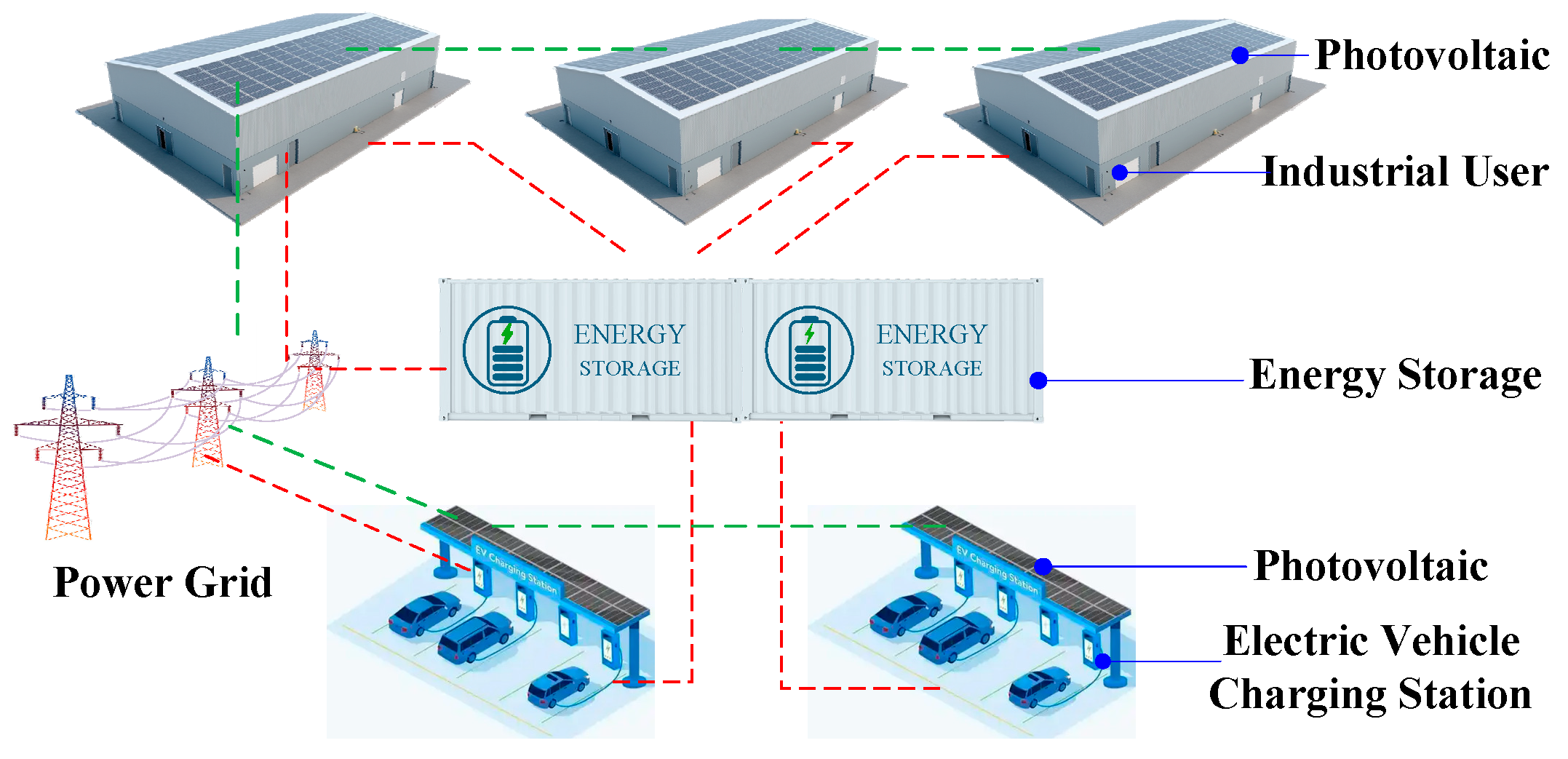
This study takes the PV-SESS-CS project constructed in a park as an example to discuss. Combined with the actual user needs of the industrial park, the optimal allocation of the energy storage capacity of the park’s PV-SESS-CS integration scheme is carried out. A schematic diagram of the park model is shown in Figure 1, including industrial users (IUs), CSs, and self-built PVs. In addition, the park users jointly invest in the construction of a SESS. Among them, users can supply power from the power grid or from SESS, and the use’s self-built PV output is preferentially supplied to its own load. When the user cannot consume, the PV will supply power to SESS or sell power to the power grid.

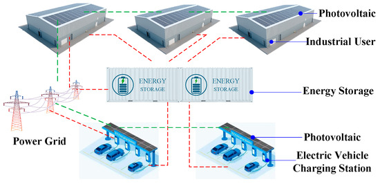
Figure 1. Schematic diagram of park model with PV-SESS-CS.

In this study, all energy users within the park are assumed to share a unified electricity account. Electricity purchases and sales are centrally managed and settled by the park operator. As a result, internal electricity transfers only consider line losses, without involving pricing between users. In addition, to avoid excessive capacity allocation caused by unrestricted peak–valley arbitrage, SESS is assumed not to sell electricity to the grid. This is because, under the current centralized settlement structure, SESS lacks the independent metering and market access required for grid electricity trading.

2.2. Construction of Shared Energy Storage Configuration Model in Park

2.2.1. Objective Function

In this study, the minimum daily operating cost of the park is taken as the goal, and the energy storage configuration model is constructed. The objective function is shown in Equation (1).

$$F=\min (C_1+C_2-C_3+C_4+C_5-C_6)$$

(1)

where $C_1$ is the initial investment cost of shared energy storage; $C_2$ is the operation and maintenance cost of shared energy storage; $C_3$ is the recycling income of shared energy storage; $C_4$ is the cost of purchasing electricity in the park; $C_5$ is the depreciation cost of energy storage battery life; $C_6$ is the carbon emission reduction benefit of the optical storage and charging system.

1.

Initial investment costs

The initial investment cost of SESS mainly includes battery cost, battery supporting equipment cost and construction cost. The initial investment cost is related to the rated power and capacity of energy storage [14], as shown below:

$$C_1={\displaystyle \frac{c_p{P}_m+c_e{E}_m}{N{D}_P}}$$

(2)

where $c_p$ and $c_e$ are the cost coefficients of unit power and unit capacity of energy storage equipment; $P_m$ is the rated power of energy storage; $E_m$ is the capacity of energy storage. According to the factory setting of the energy storage equipment, $P_m=\beta E_m$ can be obtained, where β is the maximum charge/discharge rate of the battery, representing the maximum power output per unit of energy [15]. It is used to constrain the system’s charging and discharging power. N is the service life of SESS; $D_p$ is the annual operating days of PV-SESS-CS.

2.

Operation and maintenance costs

The operation and maintenance costs of SESS mainly include labor cost, maintenance cost and replacement cost of some energy storage devices. The operation and maintenance costs are related to the rated power of the energy storage:

$$C_2={\displaystyle \frac{{{\displaystyle \sum _{n=1}^N{c}_o{P}_m\left(\frac{1+t_r}{1+d_r}\right)}}^n}{N{D}_p}}$$

(3)

where $c_o$ is the annual operation and maintenance cost coefficient of unit charging and discharging power of shared energy storage equipment; $t_r$ is the inflation rate; $d_r$ is the discount rate.

3.

Recycling income

The battery capacity of energy storage will decay with an increase in the number of cycles. When the capacity of the battery decays to a certain extent, some benefits can be obtained through echelon utilization or recycling. The recycling value of energy storage equipment is related to the initial installation cost, which is expressed as follows:

$$C_3=\gamma C_1$$

(4)

where $\gamma$ is the recycling income coefficient.

4.

Power purchase cost

The cost of purchasing electricity in the park includes the cost of IUs purchasing electricity from the grid, the cost of SESS purchasing electricity from the grid, and the profit of PV selling electricity to the grid. The specific expressions are as follows:

$$C_4=C_{\mathrm{G}rid-User}+C_{\mathrm{G}rid-ESS}-C_{PV-Grid}$$

(5)

$$C_{\mathrm{G}rid-User}={\omega }_{1,t}{\displaystyle \sum _{i=1}^5{\displaystyle \sum _{t=1}^{24}{P}_{i,t}^{\mathrm{G}rid-User}}}$$

(6)

$$C_{Grid-ESS}={\omega }_{1,t}{\displaystyle \sum _{t=1}^{24}{P}_t^{Grid-ESS}}$$

(7)

$$C_{PV-Grid}={\omega }_{2,t}{\displaystyle \sum _{i=1}^5{\displaystyle \sum _{t=1}^{24}{P}_{i,t}^{PV-Grid}}}$$

(8)

where $C_{\mathrm{G}rid-User}$ is the cost for users to purchase electricity from the power grid; $C_{\mathrm{G}rid-ESS}$ is the cost of SESS purchasing power from the grid; $C_{PV-Grid}$ is the income of PV power sales to the grid; ${\omega }_{1,t}$ is the price of electricity purchased from the grid by users and SESS at t time, and the value of t in this study is 1–24; $P_{i,t}^{\mathrm{G}rid-User}$ is the power purchased from the grid by the power user i at t time, and the values of i in this study are 1, 2, 3, 4, 5; $P_t^{Grid-ESS}$ is SESS to purchase power from the power grid at t time; ${\omega }_{2,t}$ is the electricity price of PV selling electricity to the grid at t time; $P_{i,t}^{PV-Grid}$ is the power sold to the grid by PV i at t time.

5.

Depreciation cost of energy storage life

Based on the exchange power-based energy storage life depreciation cost modeling method, the general characteristics of the depreciation process are approximated, and the fixed energy storage life depreciation cost coefficient is used for modeling and calculation. The life depreciation cost of the energy storage is [16]:

$$C_5={\displaystyle \sum _t^{24}{c}_d(P_t^{dis}+P_t^{ch})\mathsf{\Delta }t}$$

(9)

where $c_d$ is the loss cost coefficient corresponding to the unit charge and discharge amount, and the calculation method is shown in Equation (10). $P_t^{dis}$ and $P_t^{ch}$ are the discharge power and charging power of the energy storage at t time, respectively.

$$c_d={\displaystyle \frac{(C_1+C_2-C_3)N{D}_p}{L_E}}$$

(10)

In Equation (10), $L_E$ is the total charge and discharge amount in the whole lifecycle of the shared energy storage, and the calculation formula is shown in Equation (11). $N_{cyc}$ is the total number of cycles that the energy storage can cycle with $SO{C}_{\max }$ and $SO{C}_{\min }$ as the boundary.

$$L_E=(SO{C}_{\max }-SO{C}_{\min })\times E_m\times 2N_{cyc}$$

(11)

6.

Carbon emission reduction benefits

PV-SESS-CS not only significantly improves energy utilization efficiency and reduces operational costs but also offers substantial carbon reduction potential. Under China’s carbon market framework, regulated entities can offset their carbon emission quotas on a 1:1 basis using CCERs. The CCER program was officially relaunched in January 2024, and its market mechanisms are well defined; the primary market is managed by national authorities, who are responsible for the validation, registration, and issuance of CCERs for qualified projects, such as renewable energy installations, while the secondary market provides a spot trading platform where regulated enterprises can freely buy or sell CCERs to meet their compliance obligations.

Against this backdrop, PV-SESS-CS systems can reduce reliance on electricity from the conventional grid and generate verified emission reductions that qualify as CCERs, which can then be sold in the secondary market to generate revenue. The carbon emission reduction benefits of SESS in the carbon market through the CCER mechanism are shown in Equation (12). The carbon emission reduction benefits of SESS are closely related to its carbon emission reduction. The calculation method of the carbon emission reduction in SESS is shown in Equation (13):

$$C_6={\displaystyle \sum _{t=1}^{24}{K}_c{c}_c{Q}_t}$$

(12)

$$Q_t={\varphi }_c{P}_t\mathsf{\Delta }t$$

(13)

$$P_t=P_{i,t}^{PV-Grid}+P_{i,t}^{PV-User}+{\eta }^2{P}_{i,t}^{PV-ESS}$$

(14)

where $K_c$ is an indicator that characterizes the historical performance of SESS in the national Certified Voluntary Emission Reductions trading market; $c_c$ is the price coefficient of carbon emission reduction per unit participating in CCER; $Q_t$ is the emission reduction in SESS at t time; ${\varphi }_c$ is the marginal emission factor of the power grid, meaning the carbon emission reduction generated by every 1000 kWh of electricity generated by SESS; $P_t$ is the predicted emission reduction power of SESS; $P_{i,t}^{PV-User}$ is the power transmitted by PV i to user i at t time; $\eta$ is the power transmission efficiency of the tie line, and the value is 0.95; $P_{i,t}^{PV-ESS}$ is the power transmitted by PV i to SESS at t time.

2.2.2. Constraints

1.

Energy storage power station

For SESS, the discharge power of each time period should be equal to the sum of the charging power of all users stored in the time period, and the charging power of each time period should be equal to the sum of all the electricity transmitted from PV and purchased from the power grid in the time period. At the same time, the charging/discharging power of SESS at any time cannot exceed the rated power of its configuration:

$$\left\{\begin{array}{l}{P}_t^{dis}={\displaystyle \sum _{i=1}^5{P}_{i,t}^{ESS-User}}\\ P_t^{ch}=P_t^{Grid-ESS}+{\displaystyle \sum _{i=1}^5{P}_{i,t}^{PV-ESS}}\end{array}\right.$$

(15)

$$\left\{\begin{array}{l}0\le P_t^{dis}\le U_t^{dis}{P}_{\mathrm{m}}\\ 0\le P_t^{ch}\le U_t^{ch}{P}_{\mathrm{m}}\end{array}\right.$$

(16)

where $P_{i,t}^{ESS-User}$ is the power transmitted by the energy storage to the user i at t time; $U_t^{dis}$ and $U_t^{ch}$ are Boolean variables, which represent the discharge and charging state of SESS at t time. When $U_t^{dis}$ is 1, the shared energy storage is in the discharge state. Similarly, when $U_t^{ch}$ is 1, the shared energy storage is in the charging state.

Any energy storage device cannot perform charging and discharging behavior at the same time. Therefore, Equation (17) is used to constrain the charging/discharging state of shared energy storage.

$$U_t^{dis}+U_t^{ch}\le 1$$

(17)

The SOC of the energy storage battery is the ratio of its remaining power to the rated power. In order to avoid the adverse effects of overcharge or over-discharge of the energy storage battery on the battery life, in a charge/discharge cycle, the SOC of the energy storage battery needs to be limited to a certain range:

$$S{\mathrm{OC}}_{\min }\le SO{C}_t\le SO{C}_{\max }$$

(18)

where $SO{C}_{\max }$ and $SO{C}_{\min }$ are the maximum and minimum values of the state of charge of SESS, respectively; $SO{C}_t$ is the state of charge of SESS at t time.

The capacity $E_t$ of SESS at t time is determined by the charging and discharging power of the capacity $E_{t-1}$ at t − 1 time and the charging and discharging power at time t. After a charging/discharging cycle, the capacity of SESS should be equal to the initial capacity $E_0$, and d is 0.4-times its rated capacity.

$$E_t=E_{t-1}+[P_t^{ch}\eta -{\displaystyle \frac{P_t^{dis}}{\eta }}]\mathsf{\Delta }t$$

(19)

$$E_0=E_{24}=0.4E_m$$

(20)

2.

PV output

The user’s PV system needs to meet the following constraints:

$$P_{i,t}^{PV}=P_{i,t}^{PV-ESS}+P_{i,t}^{PV-User}-P_{i,t}^{PV-Grid}$$

(21)

$$0\le P_{i,t}^{PV-ESS}\le P_{lin}^{\max }$$

(22)

$$0\le P_{i,t}^{PV-User}\le P_{lin}^{\max }$$

(23)

$$0\le P_{i,t}^{PV-Grid}\le P_{lin}^{\max }$$

(24)

where $P_{i,t}^{PV}$ is the output of PV i at t time; $P_{lin}^{\max }$ is the upper limit of tie-line power, with a value of 1500 kW.

3.

User load

Users need to meet the following constraints:

$$P_{i,t}^{User}=P_{i,t}^{PV-User}+P_{i,t}^{ESS-User}+P_{i,t}^{Grid-User}$$

(25)

$$0\le P_{i,t}^{PV-User}\le P_{lin}^{\max }$$

(26)

$$0\le P_{i,t}^{ESS-User}\le P_{lin}^{\max }$$

(27)

$$0\le P_{i,t}^{Grid-User}\le P_{lin}^{\max }$$

(28)

where $P_{i,t}^{User}$ is the electricity load of user i at t time.

3. Two-Stage Robust Optimization Model and Solution Method for Shared Energy Storage Configuration in Park

In order to effectively introduce and deal with the uncertainty of PV output and EV charging load, a two-stage robust optimization model is adopted in this study. The model uses a hierarchical decision-making framework. The first stage determines the optimal configuration of SESS, and the second stage dynamically adjusts the charging and discharging strategy according to the uncertainty in actual operation. This phased optimization method can not only effectively deal with the uncertainty of PV output and EV charging load but also provide robust engineering decision support in uncertain scenarios. Therefore, we choose to build an optimal allocation model of SESS in the park based on the two-stage robust optimization model.

3.1. A Two-Stage Robust Optimization Model for Shared Energy Storage Configuration in the Park

In this study, the minimum daily operating cost of the user is the objective function, as shown in Equation (1), and the constraints to be satisfied include Equations (15)–(28). When the uncertainties of PV output and EV charging load are not considered, a deterministic optimization model of the energy storage configuration problem can be constructed, and its compact form can be expressed as a mixed integer linear programming problem.

$$\left\{\begin{array}{ll}\underset{x,y}{\min }& c^{T}y\\ s.t.& Ay\ge a\\ & By=b\\ & Dx\ge d\\ & Fx+Gy\ge f\\ & L\stackrel{⏜}{u}+Hy=h\end{array}\right.$$

(29)

where c is the coefficient column vector of the objective function; x and y are the optimization variables, and the specific expression is shown in Equation (30);A, B, C, D, F, G, L and H are the corresponding coefficient matrices under the equality and inequality constraints, respectively; a, b, d, f and h are the constant column vectors corresponding to the constraint conditions; $\stackrel{⏜}{u}$ is the corresponding predicted value of PV output and CS load in each period of time in the deterministic optimization model, and the specific expression is shown in Equation (31). Among them, the first line of the constraint condition represents the inequality constraint related to y, the second line represents the equality constraint related to y, the third line represents the inequality constraint related to x, and the fourth line represents the inequality constraint related to x and y. Line 5 represents the equality constraints related to $\stackrel{⏜}{u}$ and y.

$$\left\{\begin{array}{l}x={[U_t^{ch},U_t^{dis}]}^T\\ y={[P_t^{ch},P_t^{dis},P_t^{Grid-ESS},P_{i,t}^{PV-ESS},P_{i,t}^{ESS-User},P_{i,t}^{PV-User},P_{i,t}^{Grid-User},P_{i,t}^{PV-Grid},E_m]}^T\end{array}\right.$$

(30)

$$\stackrel{⏜}{u}={[\stackrel{⏜}{P_{1,t}^{PV}},\stackrel{⏜}{P_{2,t}^{PV}},\stackrel{⏜}{P_{3,t}^{PV}},\stackrel{⏜}{P_{4,t}^{PV}},\stackrel{⏜}{P_{5,t}^{PV}},\stackrel{⏜}{P_{4,t}^{User}},\stackrel{⏜}{P_{5,t}^{User}}]}^T$$

(31)

where $\stackrel{⏜}{P_{1,t}^{PV}},\stackrel{⏜}{P_{2,t}^{PV}},\stackrel{⏜}{P_{3,t}^{PV}},\stackrel{⏜}{P_{4,t}^{PV}},\stackrel{⏜}{P_{5,t}^{PV}}$ are the predicted values of the PV output of PV 1–5 at t time; $\stackrel{⏜}{P_{4,t}^{User}},\stackrel{⏜}{P_{5,t}^{User}}$ are the load forecasting value of CS A and CS B at t time.

In order to accurately describe the uncertainty of PV output and EV charging load, it is necessary to reasonably select the uncertainty set. Although the uncertainty set of the ellipse and cone can provide a flexible modeling method, its nonlinear structure leads to high computational complexity, a time-consuming solution process and large resource consumption. In contrast, the box uncertainty set has a linear structure, which reduces the computational complexity and ensures the efficient solution of the model. Therefore, we choose the box uncertainty set to define the fluctuation range of the two. Specifically, the dynamic box uncertainty set U of the uncertain variable u is as follows:

$$U:\left\{\begin{array}{l}u={[u_{I,t}^{PV},u_{J,t}^{User}]}^T\\ u_{i,t}^{PV}\in [\stackrel{⏜}{P_{i,t}^{PV}}-\mathsf{\Delta }{P}_{i,t}^{PV,\max },\stackrel{⏜}{P_{i,t}(t)}+\mathsf{\Delta }{P}_{i,t}^{PV,\max }]\\ u_{j,t}^{User}\in [\stackrel{⏜}{P_{j,t}^{User}}-\mathsf{\Delta }{P}_{j,t}^{User,\max },\stackrel{⏜}{P_{j,t}^{User}}+\mathsf{\Delta }{P}_{j,t}^{User,\max }]\end{array}\right.$$

(32)

where $u_{I,t}^{PV}=[u_{1,t}^{PV},u_{2,t}^{PV},u_{3,t}^{PV},u_{4,t}^{PV},u_{5,t}^{PV}]$ is the output uncertainty variable of PV 1–5 after considering uncertainty; $u_{J,t}^{User}=[u_{4,t}^{User},u_{5,t}^{User}]$ is the uncertain variable of the CS A and CS B load after considering the uncertainty; $\mathsf{\Delta }{P}_{i,t}^{PV,\max }$ is the maximum fluctuation deviation of the predicted value of PV output of PV i at t time; $\mathsf{\Delta }{P}_{j,t}^{User,\max }$ is the maximum fluctuation deviation of the load forecast value of the user j at t time.

The goal of the two-stage robust optimization model constructed in this study is to find the most economical situation of SESS capacity configuration when the uncertain variable u takes the value of the worst case in the uncertain set U, that is, to calculate the minimum cost in the worst case, as shown in Equation (33).

$$\left\{\begin{array}{ll}\underset{x}{\min }& \left\{\underset{u\in U}{\max }\underset{y\in \Omega (x,u)}{\min c^{T}y}\right\}\\ s.t.& x=(x_1,x_2,\dots \dots ,x_{2\times 24})\\ & x_n\in \left\{0,1\right\},\forall n\in (1,2,\dots \dots ,2\times 24)\end{array}\right.$$

(33)

where the first stage problem is the outer-layer min problem, and the optimized variable is x; the two-stage problem is the max–min problem of the inner layer, and the optimization variables are u and y. Among them, the minimization problem is consistent with the objective function of Equation (29), that is, to minimize the daily cost of users. Given a set of $\left(x,u\right)$, the specific value interval of the optimization variable y is $\Omega \left(x,u\right)$, as shown in Equation (34).

$$\Omega (x,u):\left\{\begin{array}{l}Ay\ge a\\ By=b\\ Dx\ge d\\ Fx+Gy\ge f\\ Lu+Hy=h\end{array}\right.$$

(34)

Therefore, when the uncertain variable u is known, Equation (33) can be simplified to the deterministic optimization model in Equation (29). The task of the second-stage max structure is to identify which of all possible scenarios will lead to the highest running cost, that is, to find the cost in the worst case.

3.2. The Solution Method of Shared Energy Storage Configuration in the Park

For the above two-stage robust optimization model, this study uses C&CG to solve it. The C&CG algorithm obtains the optimal solution of the original problem by decomposing the original problem into the main problem (MP) and the sub-problem (SP) [17]. In the process of solving the MP, the variables and constraints related to the SP are continuously introduced, which avoids the one-time processing of all constraints, thus significantly reducing the computational complexity and obtaining a more compact lower bound of the original objective function value, thus effectively reducing the number of iterations and improving the solution efficiency.

By decomposing Equation (33), the MP form obtained is:

$$\left\{\begin{array}{ll}\underset{x}{\min }& \alpha \\ s.t.& \alpha \ge c^T{y}_l\\ & A{y}_l\ge a\\ & B{y}_l=b\\ & Dx\ge d\\ & Fx+G{y}_l\ge f\\ & L{u_l}^{\ast }+H{y}_l=h\\ & \forall l\le k\end{array}\right.$$

(35)

where k is the current number of iterations; $y_l$ is the solution of the SP after the lth iteration; ${u_l}^{\ast }$ is the value of the uncertain variable u in the worst scenario found after the lth iteration.

The SP after decoupling is as follows:

$$\underset{u\in U}{\max }\underset{y\in \Omega (x,u)}{\min }{c}^{T}y$$

(36)

Although the max–min structure in the SP is complex, the minimization problem of the inner layer can be transformed into an equivalent maximization problem through dual transformation. This transformation enables the inner problem to be combined with the outer max problem. The value range of the decision variable y is given above. Now, we restate Equation (34) as follows:

$$\Omega (x,u):=\left\{\begin{array}{ll}y|& \\ Ay\ge a,& \to \gamma \\ By=b,& \to \lambda \\ Dx\ge d,& \to \nu \\ Fx+Gy\ge f,& \to \pi \\ Lu+Hy=h.& \to \beta \end{array}\right\}$$

(37)

where $\gamma$, $\lambda$, $\nu$, $\pi$, $\beta$ are the dual variables corresponding to each constraint in the minimization problem of the second stage.

After the dual transformation, the SP is transformed into a dual problem, as shown in Equation (38).

$$\left\{\begin{array}{l}\underset{u\in U,\gamma ,\lambda ,\nu ,\pi ,\beta }{\max }{a}^T\gamma +b^T\lambda +{(d-Dx)}^T\nu +{(f-Fx)}^T\pi +{(h-Lu)}^T\beta \\ s.t.A^T\gamma +B^T\lambda +G^T\pi +H^T\beta \le c^T\\ \gamma \ge 0,\lambda \in ℝ,\nu \ge 0,\pi \ge 0,\beta \in ℝ\end{array}\right.$$

(38)

The uncertain variable a corresponding to the optimal solution of the dual problem is a pole of the uncertain set U. When Equation (38) takes the maximum value, the value of the uncertain variable u should be located at the boundary of the interval described by Equation (32). In other words, if the output of the PV is set to be minimum and the load of the CS is set to be maximum, the daily cost of the user will reach the highest level, which is the so-called ‘worst scenario’. Therefore, the fluctuation range defined in Equation (32) can be rewritten as Equation (39).

$$U:\left\{\begin{array}{l}u={[u_{I,t}^{PV},u_{J,t}^{User}]}^T\\ u_{i,t}^{PV}=[\stackrel{⏜}{P_{i,t}^{PV}}-B_{i,t}^{PV}\mathsf{\Delta }{P}_{i,t}^{PV,\max }]\\ {\displaystyle \sum _{t=1}^{24}{B}_{i,t}^{PV}}\le {\mathsf{\Gamma }}_i^{PV}\\ u_{j,t}^{User}=[\stackrel{⏜}{P_{j,t}^{User}}+B_{j,t}^{User}\mathsf{\Delta }{P}_{j,t}^{User,\max }]\\ {\displaystyle \sum _{t=1}^{24}{B}_{j,t}^{User}\le {\mathsf{\Gamma }}_j^{User}}\end{array}\right.$$

(39)

where $B={[B_{i,t}^{PV},B_{j,t}^{User}]}^T$ is a binary variable. When the value is 1, the uncertain variable takes the boundary value of the corresponding period in the interval. ${\mathsf{\Gamma }}_i^{PV}$ is the uncertainty value of PV output; ${\mathsf{\Gamma }}_j^{User}$ is the uncertainty value of CS load; ${\mathsf{\Gamma }}_i^{PV}$ and ${\mathsf{\Gamma }}_j^{User}$, respectively, represent the cumulative number of PV output and CS load power reaching the boundary of the fluctuation range defined by Equation (39), and their value range is all integers. The parameter is used to adjust the conservatism of the optimal solution. The greater the value of the parameter, the greater the conservatism of the proposed scheme, and, vice versa, the greater the risk. Bringing the above uncertainty into Equation (38), a complete SP can be obtained.

$$\left\{\begin{array}{l}\underset{B,\gamma ,\lambda ,\nu ,\pi ,\beta }{\max }{a}^T\gamma +b^T\lambda +{(d-Dx)}^T\nu +{(f-Fx)}^T\pi +{[h-L(\stackrel{⏜}{u}+\mathsf{\Delta }u)]}^T\beta \\ s.t.A^T\gamma +B^T\lambda +G^T\pi +H^T\beta \le c^T\\ {\displaystyle \sum _{t=1}^{24}{B}_{i,t}^{PV}\le {\mathsf{\Gamma }}_i^{PV}}\\ {\displaystyle \sum _{t=1}^{24}{B}_{j,t}^{User}\le {\mathsf{\Gamma }}_j^{User}}\end{array}\right.$$

(40)

In the formula, $\mathsf{\Delta }u=[\mathsf{\Delta }{P}_{i,t}^{PV,\max },\mathsf{\Delta }{P}_{j,t}^{User,\max }]$ is the fluctuation range of the uncertainty of PV output and CS load.

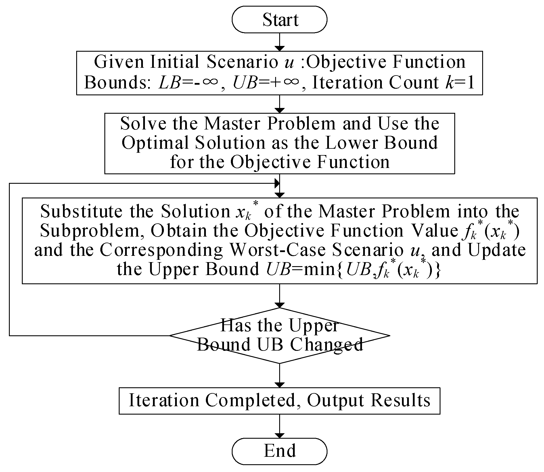
After the above derivation and transformation, the two-stage robust model is finally decomposed into the MP, as shown in Equation (35), and the SP, as shown in Equation (40), and the C&CG algorithm is used to solve the problem. The solution process of the two-stage robust optimization model is shown in Figure 2, and the specific steps are as follows.

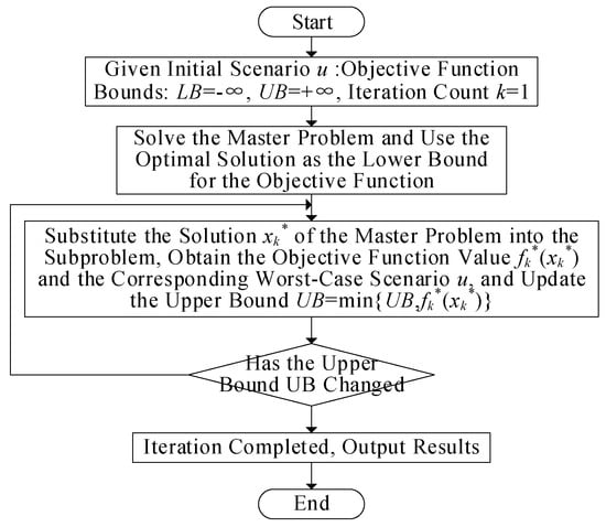
Figure 2. Solve the two-stage robust model flow chart.

(1)

The value of a set of uncertain variables u is given as the initial worst scenario, and the lower bound $LB=-\infty$, the upper bound $UB=+\infty$, and the number of iterations k = 1 corresponding to the final scheduling scheme are set.

(2)

The optimal solution $(x_k^{*},{\alpha }_k^{*},y^{1*},\cdots ,y^{k*})$ is obtained by solving the master problem in Equation (35) according to the worst scenario $u_1^{\ast }$, where the objective function value of the master problem is taken as a new lower bound $LB={\alpha }_k^{*}$;

(3)

Substitute the obtained solution $x_k^{\ast }$ of the MP into the Equation (40), solve the SP, obtain the objective function value $f_k^{*}(x_k^{*})$ of the SP and the corresponding value $u_{k+1}^{*}$ of the uncertain variable u in the worst scenario, and update the upper bound $UB=\min \left\{\left.UB,f_k^{*}(x_k^{*})\right\}\right.$;

(4)

Given that the convergence threshold of the algorithm is $\epsilon$, if $UB-LB\le \epsilon$, the iteration is stopped and the optimal solutions, $x_k^{\ast }$ and $y_k^{\ast }$, are returned. Otherwise, increase the variable $y^{k+1}$ and the following constraints:

$$\left\{\begin{array}{l}\alpha \ge c^T{y}^{k+1}\\ A{y}^{k+1}\ge a\\ B{y}^{k+1}=b\\ Dx\ge d\\ Fx+G{y}^{k+1}\ge f\\ L{u}_{k+1}^{*}+H{y}^{k+1}=h\end{array}\right.$$

(41)

4. Generation of Uncertain Scenarios of EV Charging Load and PV Output

4.1. EV Charging Load Scenario Generation

4.1.1. Charging Uncertainty Scene Generation Method

The charging behavior of a single EV owner is random and disorderly, but on the whole, the charging law will be affected by the working hours and travel rules of employees in the industrial park. Based on the statistical results of household car travel in a country for one year, this study makes a certain degree of adjustment based on the difference between daily travel and work to make it more in line with the actual situation of employees in industrial parks [18]. After adjustment, the probability density function of the owner’s arrival time in the industrial park is:

$$f_t\left(x\right)=\left\{\begin{array}{ll}{\displaystyle \frac{1}{{\sigma }_t\sqrt{2\pi }}}\exp \left(-{\displaystyle \frac{{\left(x-{\mu }_t\right)}^2}{2{{\sigma }_t}^2}}\right)& {\mu }_t-12<x<24\\ {\displaystyle \frac{1}{{\sigma }_t\sqrt{2\pi }}}\exp \left(-{\displaystyle \frac{{\left(x+24-{\mu }_t\right)}^2}{2{{\sigma }_t}^2}}\right)& 0<x<{\mu }_t-12\end{array}\right.$$

(42)

where x is the time when the owner arrives at the industrial park; ${\mu }_t$ expected value = 12.0; standard deviation ${\sigma }_t$ = 6.0. Suppose that the owner arrives at the industrial park and starts charging; the working time can be regarded as the time when the EV starts charging.

The probability density function of the daily mileage of EVs is:

$$f_s\left(x\right)={\displaystyle \frac{1}{x}}{\displaystyle \frac{1}{{\sigma }_s\sqrt{2\pi }}}\exp \left(-{\displaystyle \frac{{(\ln x-{\mu }_s)}^2}{2{{\sigma }_s}^2}}\right)$$

(43)

where d is the daily mileage of EVs; expected value ${\mu }_s$ = 3.5; standard deviation ${\sigma }_s$ = 0.88.

The battery capacity of EVs in circulation on the market presents a certain diversity. According to the collected statistical information, the battery capacity of EVs is mainly concentrated in the range of 15 kWh to 60 kWh. In order to facilitate the subsequent calculation and processing, this study selects the uniform probability distribution model in the range of 15 kWh to 60 kWh to simulate the battery capacity differences in different EVs. The probability density function is shown in Equation (44).

$$f_c(x)=\left\{\begin{array}{ll}{\displaystyle \frac{1}{45}}& 15\le x\le 60\\ 0& otherranges\end{array}\right.$$

(44)

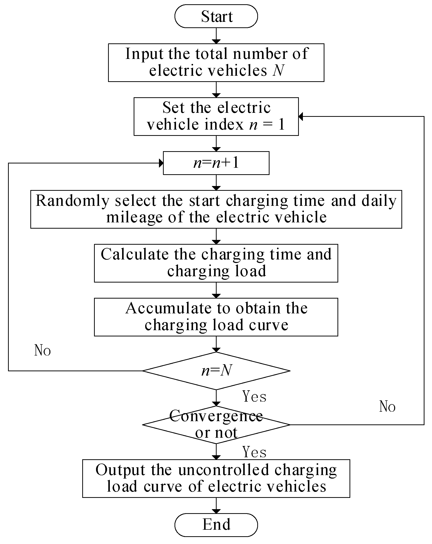
In this study, MCS is used to simulate the disorderly charging behavior of park owners. Suppose that the EV is charged once a day until it is full. In the company’s work charging scenario, EVs usually adopt a slow charging method with a more stable charging process and less impact on battery life. Therefore, the whole charging process of EVs can be approximated as constant power charging. The simulation process of the disordered charging load of EVs is shown in Figure 3, and the specific steps are as follows.

Figure 3. Flow chart of electric vehicle charging load calculation based on MCS.

(1)

Input the maximum number of simulations and the total number of electric vehicles, and initialize them.

(2)

According to the probability model mentioned above, the charging start time and daily mileage of the owner are randomly generated.

(3)

The charging power is calculated by combining the relevant parameters of the electric vehicle, and the charging load is accumulated.

(4)

After the calculation of the charging load of all electric vehicles is completed, the next simulation is carried out. After the number of simulations reaches the maximum value, the average value is taken to output the disordered charging load curve of electric vehicles.

4.1.2. Charging Load Fluctuation Curve of EV

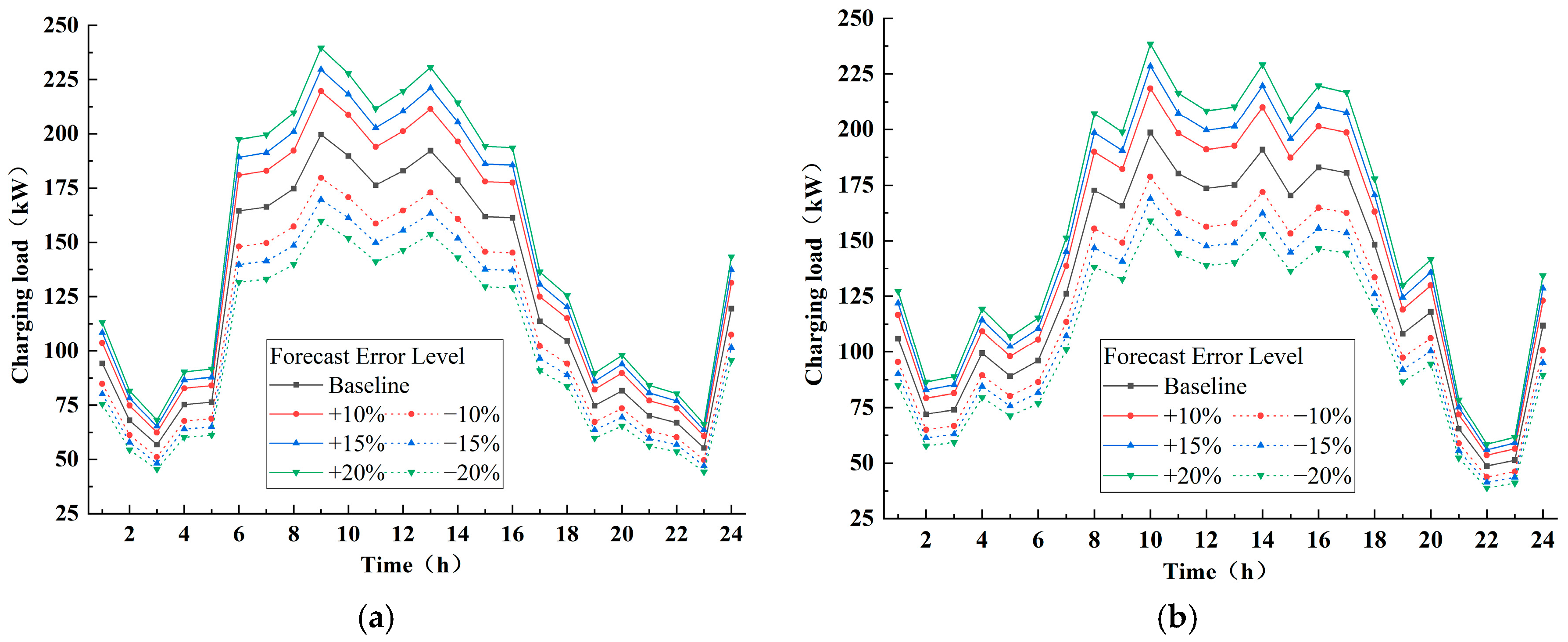
This study takes an industrial park as an example. It is assumed that there are 800 EVs in the park; two CSs, CS A and CS B, are responsible for meeting the charging needs of half of the EVs in the park. By investigating most of the EVs, we can establish that the unit power consumption of EVs is about 14 kWh/100 km, that is, 7.1 km per kilowatt-hour. Within 24 h, the charging load curves of the park CS A and CS B shown in Figure 4 can be obtained by using the method in Section 4.1.1.

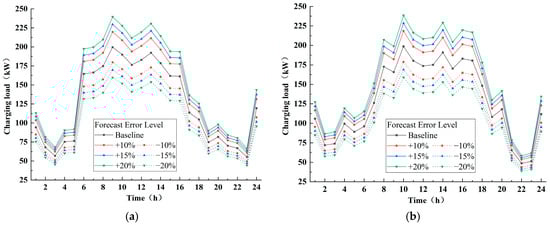
Figure 4. Predicted charging load curves of CS A and CS B under different forecast errors. (a) CS A; (b) CS B.

It can be seen from Figure 4 that the daily charging load of the CS shows a significant peak–valley characteristic: the CS will experience the highest load during the period from 8:00 to 16:00 during the day, and the charging demand reaches the peak. During the period from 19:00 p.m. to 5:00 the next day, the charging demand drops to the bottom, and the number of charging vehicles is small at this time, which is consistent with the behavior pattern of people’s daytime work.

Based on the analysis of the charging station’s operational data, it is observed that the load forecast error ${\delta }_J^{User}$ typically ranges from 5% to 15%. Therefore, in Figure 3, deviation curves of charging load forecasts are plotted for different values of ${\delta }_J^{User}$. To better reflect the fluctuations in actual operation and capture the system behavior under adverse scenarios, the values of a are set to 10%, 15%, and 20% for the simulation analysis in Section 4. For example, when ${\delta }_J^{User}=15\%$, it indicates that the actual load of the charging station fluctuates within ±15% of the forecasted value, bounded by the corresponding upper- and lower-deviation curves.

4.2. Generation of PV Output Scene in Park

4.2.1. Random Scene Generation Method of PV Output in Park

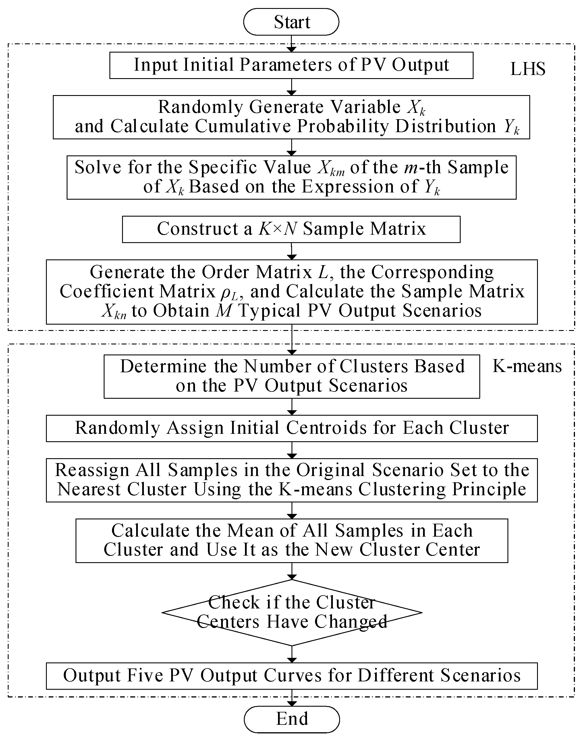
In this study, the LHS function is used to generate PV output scene samples, and the K-means algorithm is used for clustering and reduction to generate PV output data that are more in line with the actual operation needs of the park, so as to provide more accurate and targeted solutions in the scene generation of the optical storage and charging system in industrial parks [19]. The simulation process of PV output scenario generation is shown in Figure 5, and the specific steps are as follows.

Figure 5. Flow chart of PV output generated by LHS and K-means clustering.

(1)

The initial parameters of the PV system are input, and the sample values of the key variables are generated by LHS. The specific values are calculated using the cumulative probability distribution function, and the sample matrix of K*N is constructed. The initial PV output scene is generated by combining the order matrix and the coefficient matrix.

(2)

Set the number of clusters, randomly assign the initial centroid, and assign each scene to the nearest initial centroid corresponding cluster.

(3)

Calculate the mean value of the scene in each cluster as the new centroid, reassign all scenes to the cluster corresponding to the new centroid, and repeat the iteration until the centroid position is stable.

(4)

Select the scene corresponding to the final centroid of each cluster, and output the representative PV output curve for the optimization analysis of SESS.

4.2.2. PV Output Random Fluctuation Curve

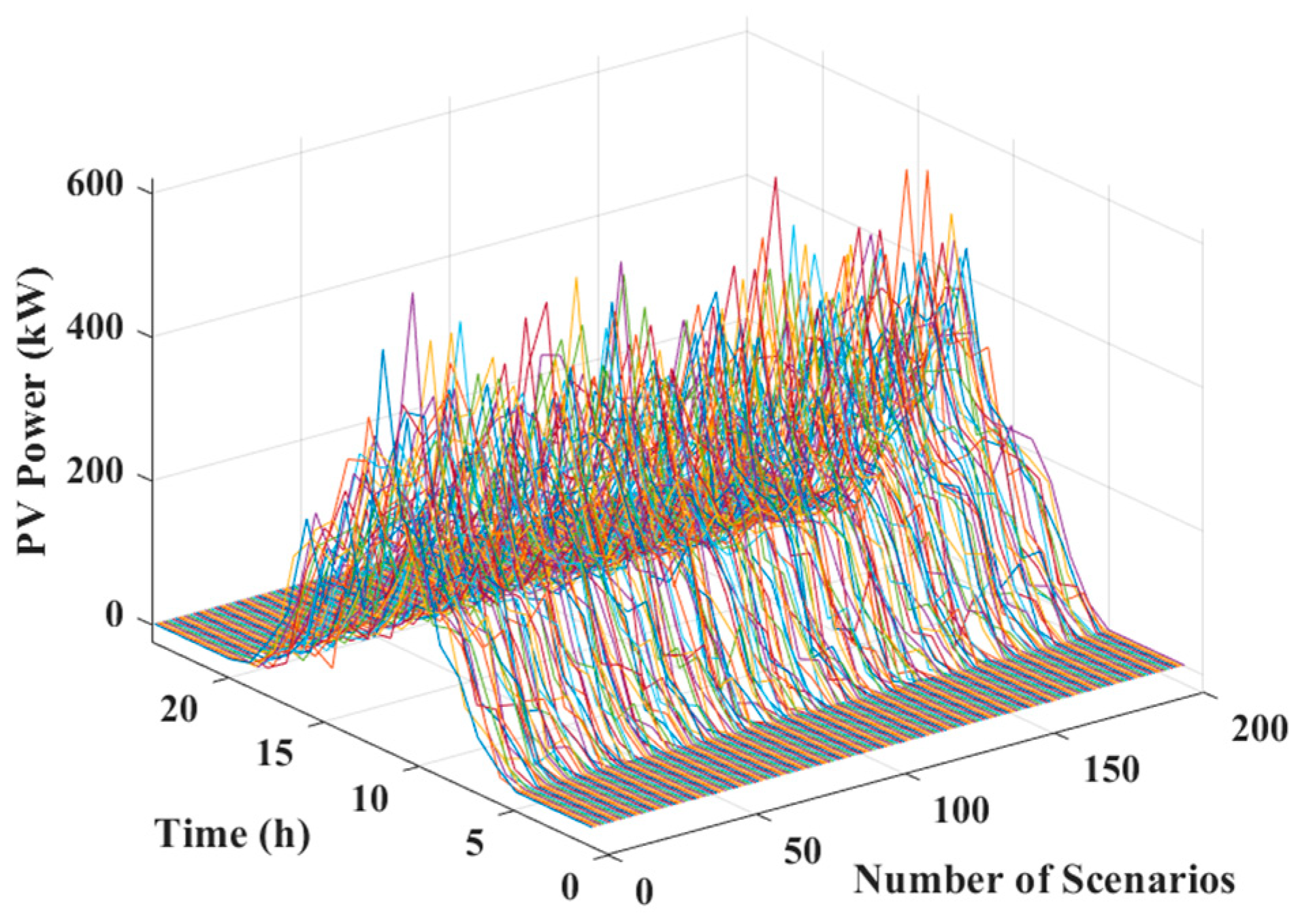
The PV output is significantly influenced by solar irradiance, and different weather conditions can lead to considerable variations in PV generation. Due to the complex and dynamic nature of daily weather changes, it is difficult to accurately classify PV output levels solely based on weather types. Therefore, this study uses the typical daily PV output curve from a real industrial park as reference data. A total of 200 PV output scenarios are generated using LHS, as shown in Figure 6.

Figure 6. PV output curves of 200 scenarios generated by LHS sampling.

For the generated large number of PV scenarios, in order to reduce the calculation time and reduce the computational complexity, the K-means clustering algorithm is selected to reduce the scenarios. The number of clustering scenarios is set to 5, and the typical daily output curves of PVs built by IU 1, IU 2, IU 3 and CS A and CS B are obtained, as shown in Figure 6. The reduced scene is similar to the original scene set, which can well characterize the change trend of PV output, and the number of reduced scenes is reduced, which reduces the computational complexity in the subsequent optimization research.

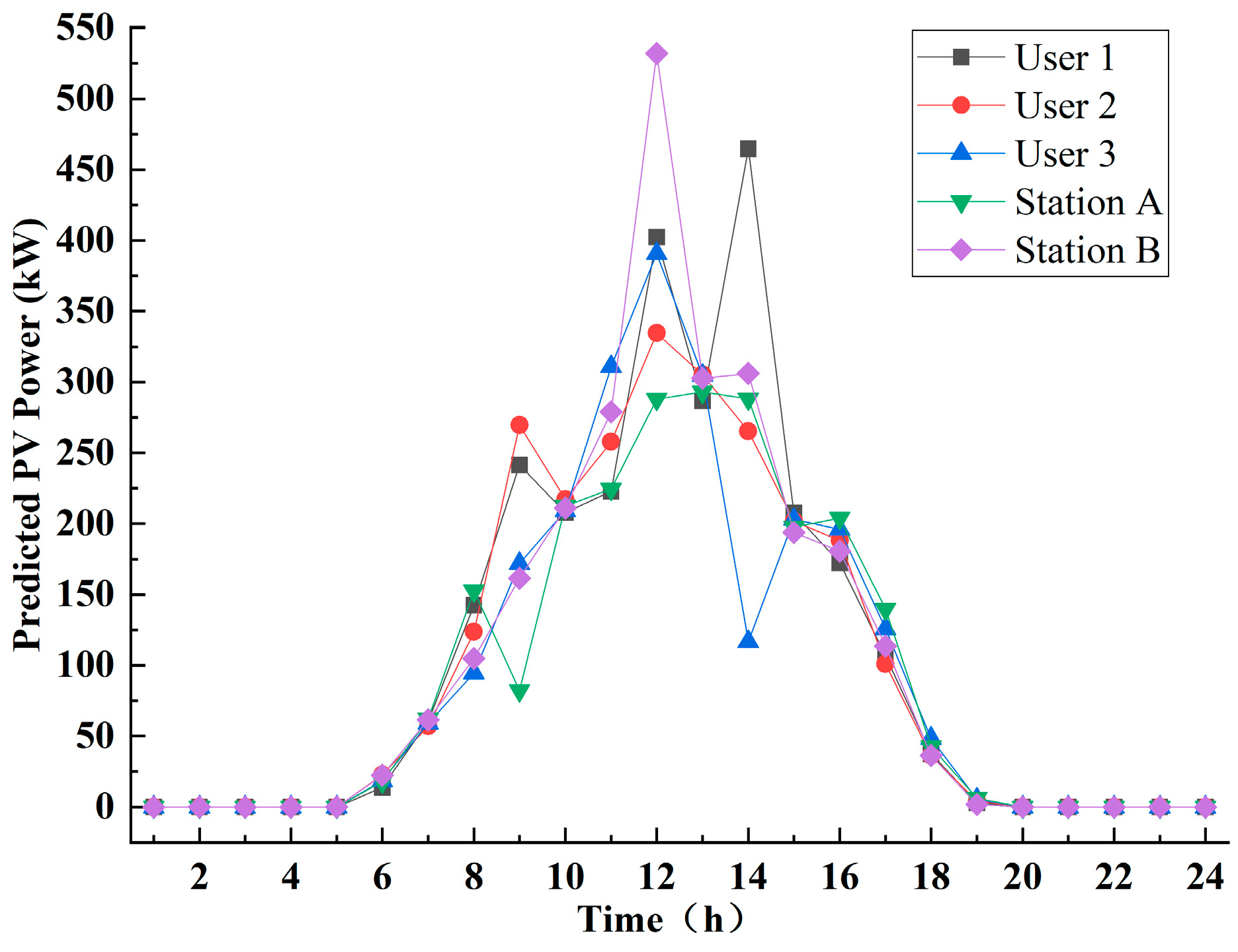
To reduce computational complexity and improve solution efficiency, this study applies the K-means clustering algorithm to perform scenario reduction on the large number of generated PV output scenarios. The number of clusters is set to five, corresponding to the number of users—three IUs (User 1, User 2, and User 3) and two CSs (Station A and Station B). The clustering results are illustrated in Figure 7.

Figure 7. Predicted PV output profiles of three IUs and two CSs.

Each cluster corresponds to the predicted PV output profile of one user, resulting in five typical PV generation curves for the three IUs and two CSs. The reduced set of representative scenarios effectively captures the variation patterns of the original dataset while significantly reducing the computational burden in the subsequent optimization model.

As shown in Figure 7, PV output is strongly correlated with solar irradiance and exhibits a clear diurnal pattern. The output remains at zero during nighttime hours when there is no sunlight and reaches its maximum around midday (12:00–14:00), when solar irradiance is strongest. The five users show similar output profiles, indicating that their PV systems follow comparable generation patterns driven by solar conditions. Meanwhile, the slight differences among the curves reflect possible variations in installation orientation, shading, or system efficiency. These results confirm that the reduced scenarios not only preserve the key temporal features of solar generation but also maintain user-specific characteristics, ensuring both representativeness and diversity for modeling purposes.

Based on the analysis of operational data from photovoltaic power stations, it is found that the PV output forecast error ${\delta }_I^{PV}$ typically ranges between 10% and 20%. To better capture the fluctuations observed in actual operation and to reflect the system’s performance under adverse conditions, this study sets the value of ${\delta }_I^{PV}$ to 15%, 20%, and 25% for the simulation analysis in Section 4. Similar to the load profiles shown in Figure 4, different values of ${\delta }_I^{PV}$ represent the fluctuation range of actual PV output under the corresponding prediction errors.

5. Case Analysis

In this study, the industrial park power grid shown in Figure 1 is taken as the research example. There are three IUs, two CSs, five self-built PV systems in the park, and one SESS is proposed to be configured. The validity of the shared energy storage configuration model and solution algorithm for low-carbon operation of the park considering the uncertainty of PV output and EV charging proposed in this study is verified by setting the original parameters.

5.1. Parameter Settings

In this study, three IUs and two CSs are selected for example analysis. The typical daily load curves of the three IUs are known, as shown in Figure 8. In addition, the forecasted load curves for the two CSs were generated in Section 4.1.2, as shown in Figure 4. The predicted PV output curves for the three IUs and two CSs were generated in Section 4.2.2, as illustrated in Figure 7. The optimization model is solved using the Gurobi solver from MATLAB R2023b.

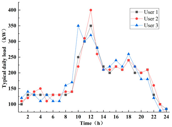
Figure 8. Typical daily load curves of IU 1, IU 2 and IU 3.

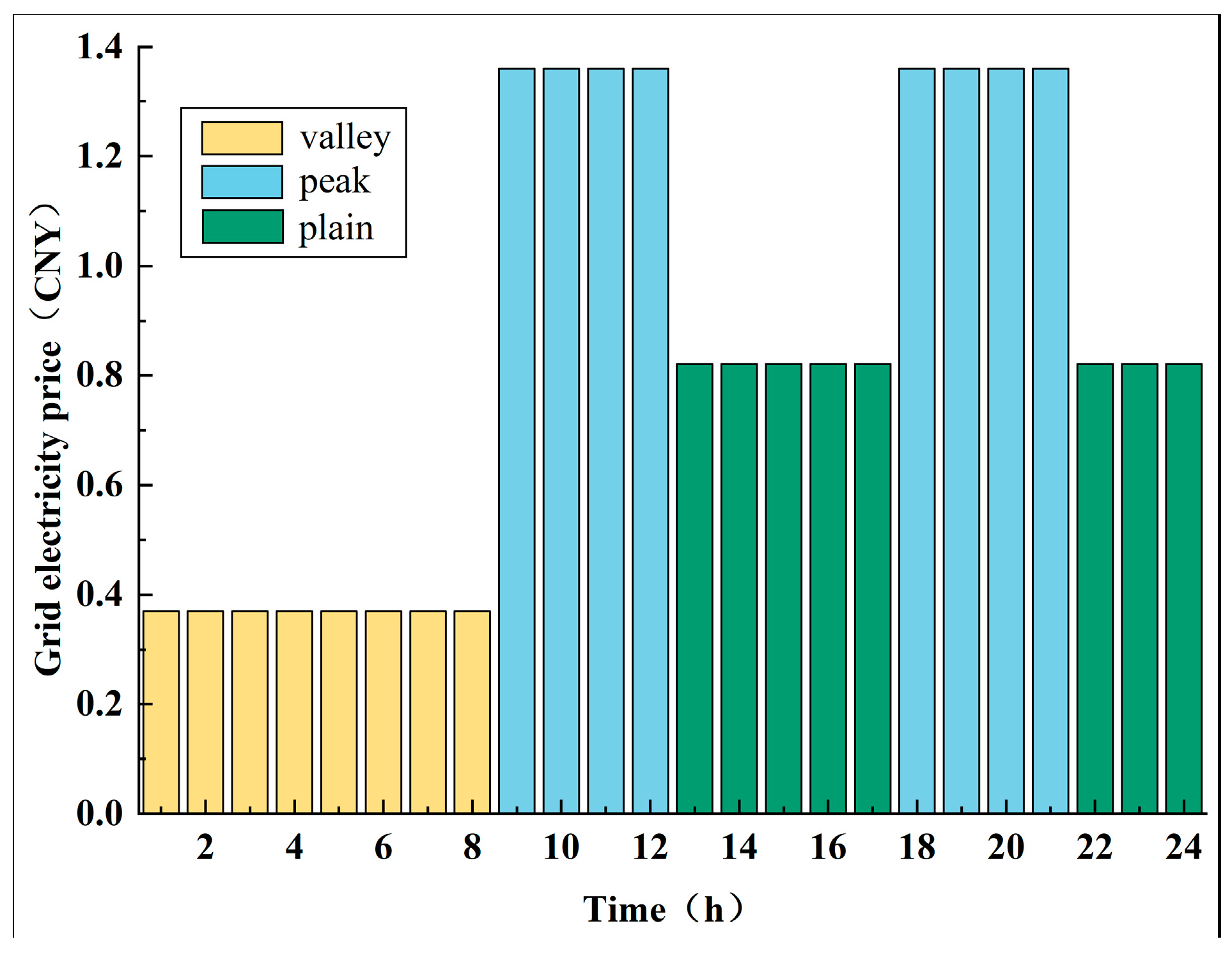
The specific parameters [20] are listed in Table 1. The grid marginal emission factor ${\varphi }_c$ is set to $7.568\times {10}^{-4}$ t CO₂/kWh, based on the average marginal emission factor of China’s national power grid in a given year (refer to the Research on the Calculation Method of Baseline and Marginal Emission Factors for Regional Power Grids in China, China Electricity Council, or relevant statistical reports). The carbon price parameter $c_c$ is based on the average daily transaction price of the first batch of CCERs following the resumption of registration in the national voluntary greenhouse gas emissions trading market. A relatively conservative low-end value of 80.5 CNY/t CO₂ is adopted [21]. The time-of-use electricity price of IUs, CSs and SESS in the park to purchase electricity from the power grid is shown in Figure 9, and the selling price of PV to the power grid is set to 0.4 CNY/kWh.

Table 1. Values of each parameter.

Parameter	Values and Units	Parameter	Values and Units
cp	60 CNY/kW	tr	0.7%
ce	1100 CNY/kWh	dr	8%
c0	87 CNY/kW	γ	0.3
SOCmax	0.9	$\beta$	0.5
SOCmin	0.1	cd	0.02 CNY/kW
N	10 years	${\varphi }_c$	7.568 × 10−4 t CO2/kWh
Dp	350 days	$c_c$	80.45 CNY/t CO2

Figure 9. Time-of-use price diagram of purchasing electricity from power grid.

5.2. Analysis of Results

Based on the previous analysis and research on the operation data of PV power stations and CSs, the PV prediction error a is set to be 15% and the load prediction error a is set to be 10%, so as to accurately reflect the uncertainty in actual operation and evaluate the robustness of the system. In addition, in order to further highlight the improvement in the energy efficiency of the park due to carbon emission reductions, this study sets up two comparative scenarios as follows:

Scenario 1: Optimal configuration model of energy storage system considering source-load uncertainty;

Scenario 2: Optimal configuration model of energy storage system considering source-load uncertainty and carbon emission reduction benefits.

The energy storage module needs to be configured in a gradient manner in practical applications, and 50 kWh is a common standard module capacity in the current energy storage market, which is in line with the standardized design of most energy storage systems. Therefore, the subsequent energy storage capacity is designed under step optimization; that is, the energy storage capacity with different uncertain values is 50 kWh as the capacity unit of each gradient.

The uncertainties in PV output and EV charging load impact both the daily operating cost and the storage capacity configuration of the park. Under the condition where the parameter is set as $\mathsf{\Gamma }={\mathsf{\Gamma }}_J^{User}=2{\mathsf{\Gamma }}_I^{PV}$, four simulation cases are constructed for Scenario 1 and Scenario 2 [22], respectively, and the results are shown in Table 2.

Table 2. Daily user cost and energy storage capacity under different uncertainty values.

Uncertainty Value	Scenario 1			Scenario 2
	F/CNY	Em/kWh	C6/CNY	F/CNY	Em/kWh	C6/CNY
${\mathsf{\Gamma }}_I^{PV}=0,{\mathsf{\Gamma }}_J^{User}=0$	6495.8	4050	/	5880.4	4050	656.49
${\mathsf{\Gamma }}_I^{PV}=3,{\mathsf{\Gamma }}_J^{User}=6$	7000.3	4050	/	6393.3	4050	637.36
${\mathsf{\Gamma }}_I^{PV}=6,{\mathsf{\Gamma }}_J^{User}=12$	7433.1	4100	/	6830.7	4100	632.83
${\mathsf{\Gamma }}_I^{PV}=12,{\mathsf{\Gamma }}_J^{User}=24$	7966.0	4200	/	7389.9	4200	602.40

When the uncertainty parameter is equal to 0, the two-stage robust optimization model is equivalent to deterministic optimization. It can be seen from Table 2 that with an increase in PV and load uncertainty, the daily cost and energy storage capacity configuration of users are also improved accordingly. In particular, in Scenario 1 and Scenario 2, when the uncertainty value changes from ${\mathsf{\Gamma }}_I^{PV}=0,{\mathsf{\Gamma }}_J^{User}=0$ to ${\mathsf{\Gamma }}_I^{PV}=3,{\mathsf{\Gamma }}_J^{User}=6$, the user’s daily cost increases, but the energy storage capacity configuration results are consistent, because this study considers the energy storage gradient configuration problem. If this problem is ignored, the energy storage capacity configuration will also increase. Therefore, when the park formulates its day-ahead scheduling plan, the more uncertain factors included, the more conservative the plan is, resulting in increased costs; on the contrary, if the consideration of uncertainty is reduced, although the cost can be reduced, the risk of the scheme will increase. By comparing Scenario 1 and Scenario 2, it can be seen that when ${\mathsf{\Gamma }}_I^{PV}$ and ${\mathsf{\Gamma }}_J^{User}$ take different values, although the energy storage capacity configuration results are the same, the daily operating cost of Scenario 2 is always lower than the daily operating cost of Scenario 1, which is related to Scenario 2. After considering carbon emission reduction, it affects the daily operation strategy of SCs and obtains additional carbon emission reduction benefits.

The larger the $\mathsf{\Gamma }$ value is, the more time periods the PV output takes to the minimum value of the prediction interval and the CS load takes to the maximum value of the prediction interval. Therefore, the power shortage of the power users in the park increases accordingly, and the power surplus decreases accordingly, resulting in a continuous increase in electricity purchase and a continuous decrease in electricity sales. The changes in electricity purchase and sales of power users in the park with $\mathsf{\Gamma }$ value are shown in Table 3.

Table 3. User’s electricity purchase and sales and PV electricity sales under different uncertainty values.

Scenario	1				2
Uncertainty Value	${\mathit{E}}_{\mathit{U}\mathit{s}\mathit{e}\mathit{r}-\mathit{G}\mathit{r}\mathit{i}\mathit{d}}$/kWh	${\mathit{E}}_{\mathit{P}\mathit{V}-\mathit{G}\mathit{r}\mathit{i}\mathit{d}}$/kWh	${\mathit{E}}_{\mathit{P}\mathit{V}-\mathit{E}\mathit{S}\mathit{S}}$/kWh	${\mathit{E}}_{\mathit{P}\mathit{V}-\mathit{U}\mathit{s}\mathit{e}\mathit{r}}$/kWh	${\mathit{E}}_{\mathit{U}\mathit{s}\mathit{e}\mathit{r}-\mathit{G}\mathit{r}\mathit{i}\mathit{d}}$/kWh	${\mathit{E}}_{\mathit{P}\mathit{V}-\mathit{G}\mathit{r}\mathit{i}\mathit{d}}$/kWh	${\mathit{E}}_{\mathit{P}\mathit{V}-\mathit{E}\mathit{S}\mathit{S}}$/kWh	${\mathit{E}}_{\mathit{P}\mathit{V}-\mathit{U}\mathit{s}\mathit{e}\mathit{r}}$/kWh
${\mathsf{\Gamma }}_I^{PV}=0,{\mathsf{\Gamma }}_J^{User}=0$	6763.6	2406.9	584.2	8936.8	5763.2	1054.3	934.9	9938.7
${\mathsf{\Gamma }}_I^{PV}=3,{\mathsf{\Gamma }}_J^{User}=6$	6983.9	1655.6	667.5	8843.0	5881.2	641.3	579.1	9945.7
${\mathsf{\Gamma }}_I^{PV}=6,{\mathsf{\Gamma }}_J^{User}=12$	7228.6	1209.3	827.3	8627.7	6160.8	195.0	773.7	9695.6
${\mathsf{\Gamma }}_I^{PV}=12,{\mathsf{\Gamma }}_J^{User}=24$	7725.3	1069.6	894.2	8192.5	6662.6	193.1	708.0	9255.2

Where $E_{User-Grid}$ is the amount of electricity purchased by users from the grid; $E_{PV-Grid}$ is the amount of electricity sold by PV to the grid; $E_{PV-ESS}$ is the power supply of PV to energy storage; $E_{PV-User}$ is the power of PV to IUs and CSs.

It can be seen from Table 3 that with an increase in the uncertainty value, the amount of electricity purchased by users from the power grid is increasing, and the amount of electricity directly supplied by PV output to IUs and CSs is decreasing, which leads to an increase in user cost. This is because as the $\mathsf{\Gamma }$ value increases, the PV output decreases, the CS load increases, the power gap increases, and the worst-case scenario becomes worse. The PV output gradually fails to meet the user’s needs, and the user’s electricity sales continue to decrease. External purchases continue to rise, resulting in rising costs. Comparing Scenario 1 and Scenario 2, it can be seen that when ${\mathsf{\Gamma }}_I^{PV}$ and ${\mathsf{\Gamma }}_J^{User}$ take different values, Scenario 2 significantly reduces the amount of electricity purchased from the grid and sold to the grid compared with Scenario 1, and the PV output directly supplies users and CSs. The amount of electricity increased significantly, and the park gave priority to the use of PV output to supply itself, achieving local consumption of PV output and reducing the impact on grid stability.

In addition to the uncertainty value, the error of power prediction will also have a certain impact on the economy. At ${\mathsf{\Gamma }}_I^{PV}=6$ and ${\mathsf{\Gamma }}_J^{User}=12$, the impact of different prediction errors on costs is shown in Table 4.

Table 4. User daily cost and energy storage capacity configuration under different prediction errors.

Scenario	1			2
Prediction Error	F/CNY	Em/kWh	C6/CNY	F/CNY	Em/kWh	C6/CNY
${\delta }_I^{PV}=15\%,{\delta }_J^{User}=10\%$	7433.1	4100	/	6830.7	4100	632.83
${\delta }_I^{PV}=20\%,{\delta }_J^{User}=15\%$	7957.1	4100	/	7376.1	4100	611.39
${\delta }_I^{PV}=25\%,{\delta }_J^{User}=20\%$	8480.1	4100	/	7931.7	4100	578.83

From Table 4, it can be seen that with an increase in prediction error, the daily cost of users continues to increase, but the energy storage capacity configuration remains unchanged. This is not only because this study considers the energy storage gradient configuration problem but also because the prediction error is too large, resulting in a large power shortage. Therefore, the park tends to increase external power purchase rather than excessive configuration of energy storage capacity. When formulating its day-ahead scheduling plan in the park, the greater the prediction error considered, the more conservative the plan is, resulting in increased costs; on the contrary, if the consideration of prediction error is reduced, although the cost can be reduced, the risk of the scheme will also increase. Comparing Scenario 1 and Scenario 2, it can be seen that when ${\delta }_I^{PV}$ and ${\delta }_J^{User}$ take different values, the daily operating cost of Scenario 2 is greatly increased compared with Scenario 1. This is related to the fact that Scenario 2 considers carbon emission reduction, which affects the daily operation strategy of CSs and obtains additional carbon emission reduction benefits.

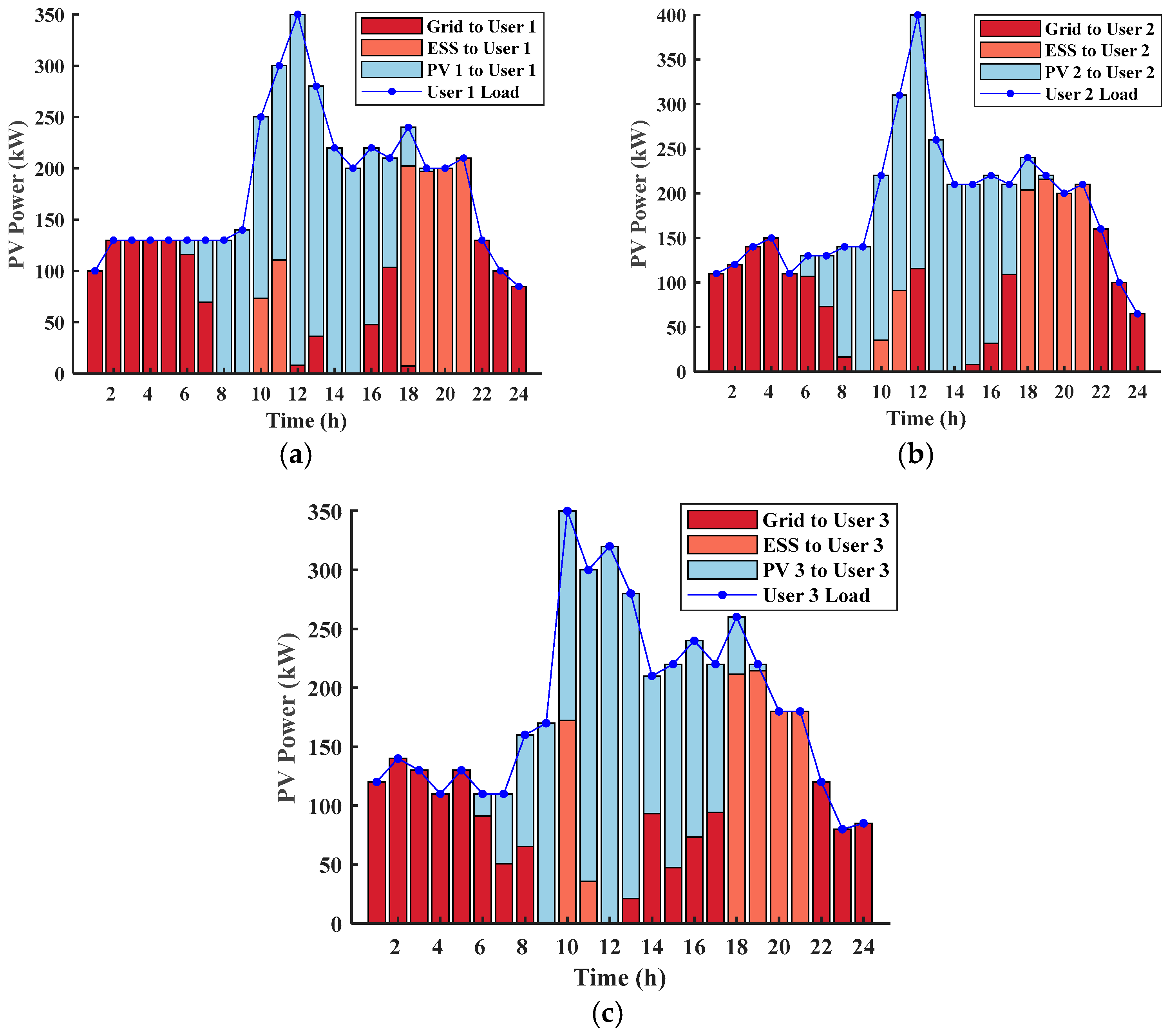
Taking ${\mathsf{\Gamma }}_I^{PV}=6,{\mathsf{\Gamma }}_J^{User}=12$, ${\delta }_I^{PV}=15\%,{\delta }_J^{User}=10\%$ as an example, after the model is solved, the load of the CS is adjusted to the maximum value of the load prediction range, and the power generation of the PV system is set to the minimum value in the predicted value, so that the power shortage becomes the largest, that is, the worst scenario. At this time, the power balance of IU 1, IU 2, and IU 3 is shown in Figure 10, and the power balance of CS A and CS B is shown in Figure 11.

Figure 10. Power balance diagrams of IU 1, IU 2 and IU 3. (a) IU 1; (b) IU 2; (c) IU 3.

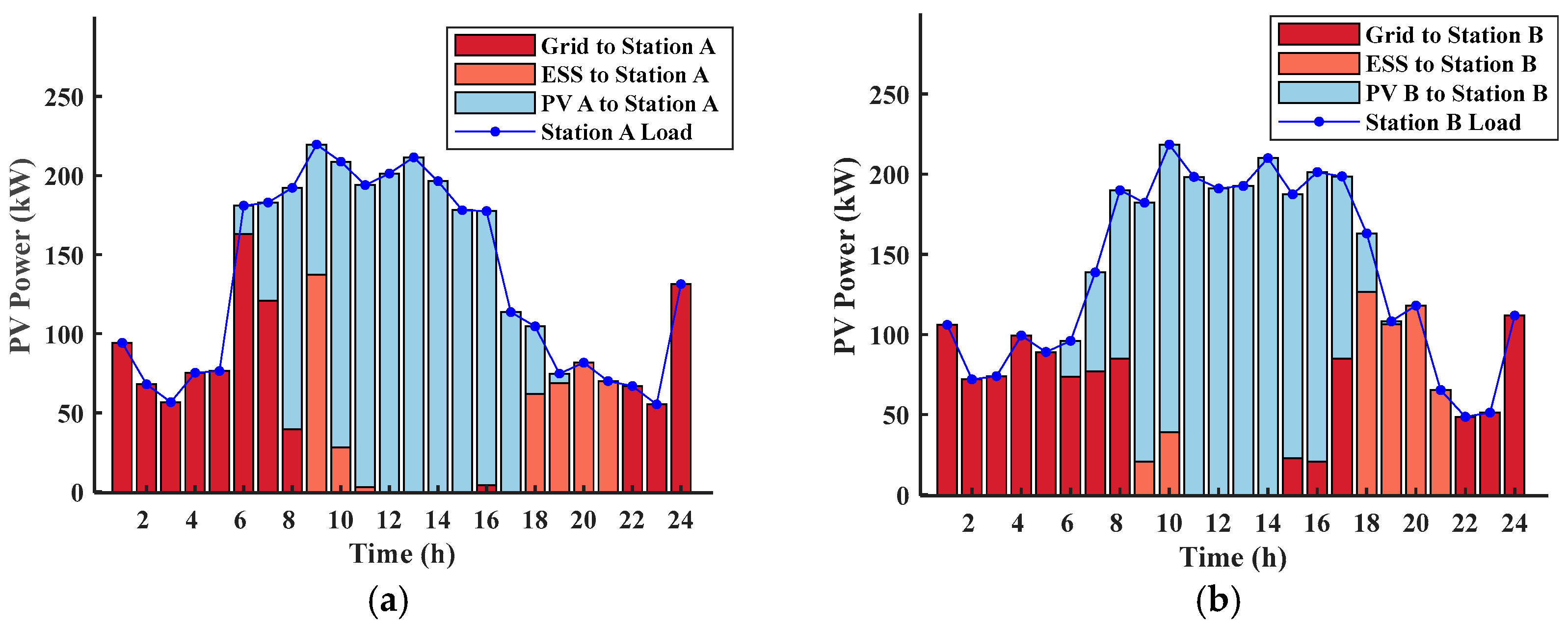
Figure 11. Power balance diagrams of CS A and CS B. (a) CS A; (b) CS B.

It can be seen from Figure 10 that in order to achieve better cost-effectiveness, each user preferentially uses its own PV power supply. Particularly at noon, the PV output can basically cover the power load of IU 1, IU 2 and IU 3. After meeting the industrial users’ demand, the surplus PV generation is used either to charge the SESS or to be sold to the grid. At 10 h, 11 h and 18–21 h, the PV output is insufficient. Due to the high electricity price from the power grid, IU 1, IU 2 and IU 3 tend to use the power of SESS. This practice is also consistent with the user’s electricity consumption habits.

Figure 11 shows a power balance diagram of the two CSs. At noon, the PV output power is greater than the power load of the CS. After the PV meets the load of the CS, the excess power will be delivered to the energy storage station or sold to the grid. When 18 h–21 h is the evening peak of electricity consumption, the electricity purchase price from the power grid is higher, and the CS preferentially uses the power of SESS to realize the cyclic scheduling of energy. When SESS is exhausted or the electricity price is reduced, the power grid is used for power supply. From the above analysis, it can be seen that the use of SESS in the peak load period of the power grid is helpful to reduce the pressure on the power grid and optimize the operation of the whole power system.

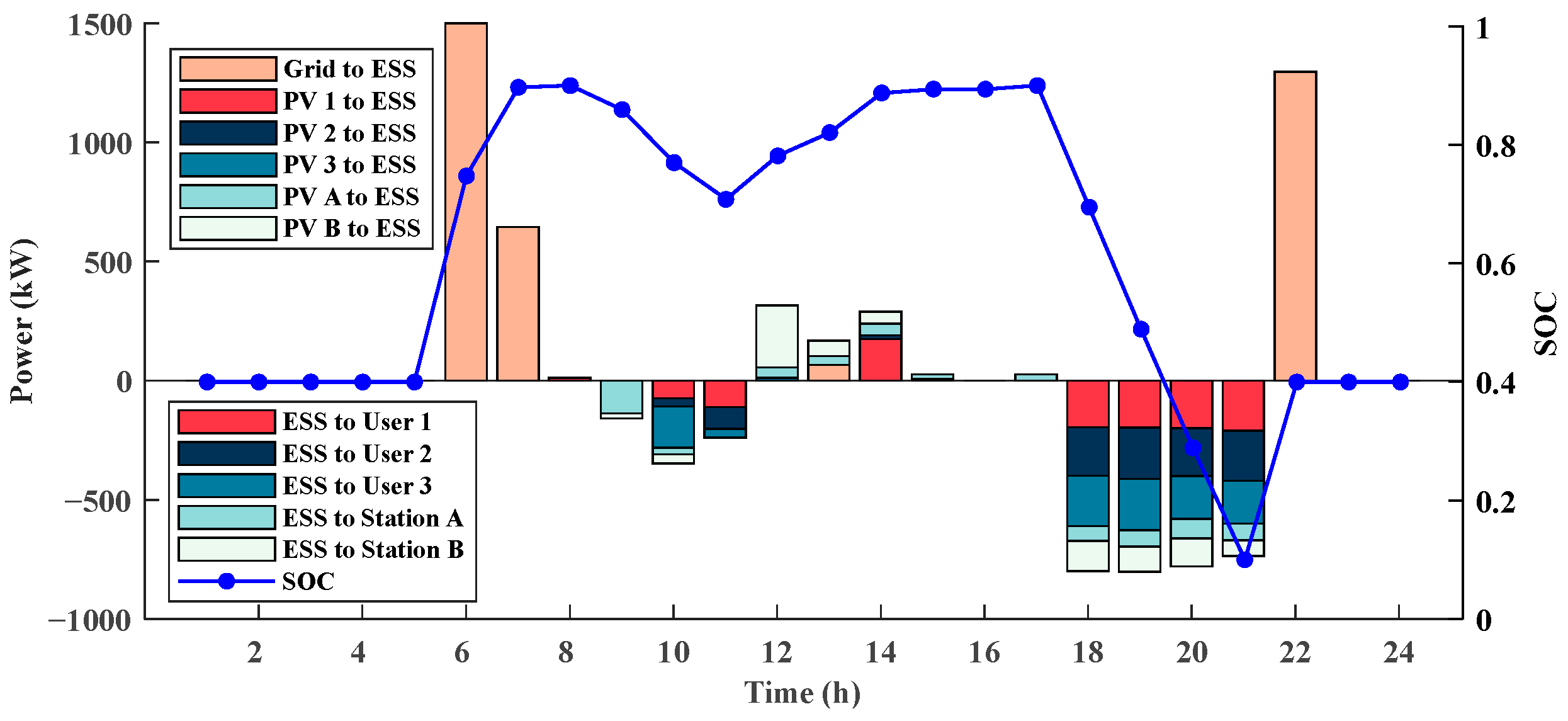
Figure 12 shows a charging and discharging power accumulation diagram of SESS and the state of the charge curve of SESS. When SESS is charged, the power value is positive and negative when discharged.

Figure 12. Charging and discharging power and state of charge curve of SESS.

It can be seen from Figure 12 that under the time-of-use electricity price mechanism, SESS purchases a large amount of electricity from the power grid at 6 h, 7 h, and 22 h, and discharges at 9–11 h and 18–21 h, thereby storing the electricity during the valley electricity price period and selling it during the peak electricity price period, effectively reducing the cost of purchasing electricity. Because the load peak period of power users (10:00–18:00) and the load peak period of CSs (6:00–17:00) match the peak period of PV output (10:00–15:00) in time, the power supply of the PV system to SESS is not significant. However, it can also collect a small amount of surplus power during the peak period of PV output and release this power during the peak period of CS load, which improves the energy utilization efficiency, cuts the peak and fills the valley, improves the economic benefit and enhances the stability of the power grid.

To evaluate the impact of storage cost variations on system performance, a sensitivity analysis was conducted under different values of the unit capacity cost coefficient $c_e$. Since the initial investment of the storage system is mainly influenced by the price of battery cells, which is directly reflected in the parameter $c_e$, 1100 CNY/kWh was taken as the baseline, with a step size of 100 CNY/kWh in the range of 900 to 1200 CNY/kWh. The effects on users’ daily operating costs and the configuration of storage capacity are shown in Table 5.

Table 5. Daily operating cost and storage capacity configuration under different unit capacity costs.

${\mathit{c}}_{\mathit{e}}$ CNY/kWh	Scenario 1		Scenario 2
	F/CNY	Em/kWh	F/CNY	Em/kWh
900	7128.5	4100	6526.1	4100
1000	7281.0	4100	6678.6	4100
1100	7433.1	4100	6830.7	4100
1200	7585.6	4100	6983.2	4100

As shown in Table 5, with an increase in the unit cost of storage capacity $c_e$, the park’s daily operating cost steadily rises, while the configured storage capacity remains fixed at 4100 kWh. This outcome is primarily due to the stepwise storage configuration adopted in this study, where capacity adjustments follow a 50 kWh increment, and the current cost range does not trigger a change in the optimal sizing threshold. In addition, further reducing the storage size to lower investment costs would significantly compromise the system’s flexibility and increase reliance on grid electricity, thereby diminishing overall economic performance. This result indicates that, within a certain cost range, the configured storage capacity remains stable and robust.

Table 6 shows the benefits of Scenario 1 and Scenario 2 in terms of electric energy and carbon trading. The economic and environmental benefits of the two shared energy storage configuration scenarios are compared and analyzed, and the optimization effect of carbon emission reduction benefits on the operation strategy and energy storage configuration of the park’s SESS is clarified.

Table 6. Income comparison between Scenario 1 and Scenario 2.

Scenario	$\mathit{c}\mathit{o}\mathit{s}{\mathit{t}}_{\mathit{b}\mathit{u}\mathit{y}}$/CNY	${\mathit{W}}_{\mathit{C}\mathit{E}\mathit{R}}$/t	${\mathit{W}}_{\mathit{S}\mathit{C}\mathit{R}}$/t	C6/CNY	C5/CNY	F/CNY
1	5195.7	7.09	3.00	/	162.85	7433.1
2	5226.1	7.87	3.33	632.83	162.85	6830.7

where $\cos t_{buy}$ is the purchase cost of users and energy storage from the grid; $W_{CER}$ is the carbon emission reduction; $W_{SCR}$ is the solar energy instead of standard coal quantity.

From Table 6, it can be seen that the daily operation cost of SESS under Scenario 1 is CNY 7433.1, and the daily operation cost under Scenario 2 is CNY 6830.7, which is 8.10% lower than that of Scenario 1. Among them, the power grid purchase cost increased by CNY 30.4, but the carbon emission reduction benefit of SESS in the carbon market was CNY 632.83. It can be seen that in the case of Scenario 1, the SESS can save a total of CNY 602.4 per day. Within the 10-year service life of energy storage, each user can save about CNY 2.1084 million. In addition, the carbon emission reduction in SESS under Scenario 2 is 11.00% higher than that under Scenario 1. The daily operation can reduce 0.68 t of carbon emissions and save 0.33 t of standard coal (assuming that the mass of 1000 kWh PV output replacing standard coal is 0.32 t).

In summary, Scenario 2 is significantly better than Scenario 1. By incorporating carbon emission reduction benefits into the optimization objectives, not only can the economic benefits of photovoltaic charging stations be effectively improved but, also, the operation strategy of energy storage systems can be effectively optimized without relying on mandatory emission constraints, achieving a synergistic improvement in environmental and economic benefits. This market-based emission reduction pathway not only validates the guiding role of carbon price signals in the construction of low-carbon power systems but also provides practical examples for promoting the consumption of renewable energy and reducing carbon emissions through economic incentives. It has important reference value for promoting the green and low-carbon transformation of the power industry.

6. Conclusions

Aiming at the uncertainty of photovoltaic output and charging station load, a low-carbon park shared energy storage optimization configuration method considering the uncertainty of photovoltaic output and electric vehicle charging is proposed. By analyzing the collaborative operation characteristics of industrial users in the park, self-built photovoltaic and shared energy storage power stations in electric vehicle charging stations, and constructing industrial park operation scenarios, the optimization configuration of energy storage capacity is achieved. The proposed model takes into account the uncertainty of photovoltaic output and charging station load. By solving the two-stage robust optimization model, the park can achieve the energy storage configuration with the minimum system operating cost in the worst-case scenario. By adjusting uncertain parameters and predicting error values, the conservatism of configuration schemes can be flexibly adjusted, which is beneficial for industrial parks to make reasonable choices between operating costs and risks. The calculation results show that the construction of shared energy storage is significantly better than the scheme without energy storage configuration. Shared energy storage can not only significantly reduce operating costs but also effectively suppress the adverse effects of source load fluctuations, increase the operating efficiency and reliability of photovoltaic systems, and reduce energy waste. By incorporating carbon emission reduction benefits into optimization objectives, this study’s scheme can effectively reduce carbon dioxide emissions, improve carbon emission reduction levels, guide energy storage systems to optimize their operational strategies, reduce operating costs, and achieve a synergistic improvement in environmental and economic benefits.

References

- Sarda, J.; Patel, N.; Patel, H.; Vaghela, R.; Brahma, B.; Bhoi, A.K.; Barsocchi, P. A Review of the Electric Vehicle Charging Technology, Impact on Grid Integration, Policy Consequences, Challenges and Future Trends. Energy Rep. 2024, 12, 5671–5692. [Google Scholar] [CrossRef]
- Yao, M.; Da, D.; Lu, X.; Wang, Y. A Review of Capacity Allocation and Control Strategies for Electric Vehicle Charging Stations with Integrated Photovoltaic and Energy Storage Systems. World Electr. Veh. J. 2024, 15, 101. [Google Scholar] [CrossRef]
- Yang, M.; Zhang, L.; Zhao, Z.; Wang, L. Comprehensive Benefits Analysis of Electric Vehicle Charging Station Integrated Photovoltaic and Energy Storage. J. Clean. Prod. 2021, 302, 126967. [Google Scholar] [CrossRef]
- Luo, J.; Fan, F.; Tai, N.; Chen, Z.; Pu, C.; Zhang, X. Low-Carbon Economic Optimization for Park Integrated Energy System Considering Multi-Network Integration. In Proceedings of the 2023 IEEE/IAS Industrial and Commercial Power System Asia (I&CPS Asia), Chongqing, China, 7–9 July 2023; pp. 2160–2165. [Google Scholar]
- Zhu, X.; Yang, J.; Pan, X.; Li, G.; Rao, Y. Regional Integrated Energy System Energy Management in an Industrial Park Considering Energy Stepped Utilization. Energy 2020, 201, 117589. [Google Scholar] [CrossRef]
- Alshareef, R.S.; Maghrabie, H.M. Building-Integrated Photovoltaics with Energy Storage Systems—A Comprehensive Review. J. Energy Storage 2025, 116, 115916. [Google Scholar] [CrossRef]
- Chen, C.; Sun, H.; Shen, X.; Guo, Y.; Guo, Q.; Xia, T. Two-Stage Robust Planning-Operation Co-Optimization of Energy Hub Considering Precise Energy Storage Economic Model. Appl. Energy 2019, 252, 113372. [Google Scholar] [CrossRef]
- Zhou, S.; Han, Y.; Mahmoud, K.; Darwish, M.M.F.; Lehtonen, M.; Yang, P.; Zalhaf, A.S. A Novel Unified Planning Model for Distributed Generation and Electric Vehicle Charging Station Considering Multi-Uncertainties and Battery Degradation. Appl. Energy 2023, 348, 121566. [Google Scholar] [CrossRef]
- Liu, Z.; Wu, J.; Cui, S.; Zhu, R. An Energy Collaboration Framework Considering Community Energy Storage and Photovoltaic Charging Station Clusters. J. Energy Storage 2025, 116, 115976. [Google Scholar] [CrossRef]
- Xu, T.; Ren, Y.; Guo, L.; Wang, X.; Liang, L.; Wu, Y. Multi-Objective Robust Optimization of Active Distribution Networks Considering Uncertainties of Photovoltaic. Int. J. Electr. Power Energy Syst. 2021, 133, 107197. [Google Scholar] [CrossRef]
- Yang, N.; Xu, G.; Fei, Z.; Li, Z.; Du, L.; Guerrero, J.M.; Huang, Y.; Yan, J.; Xing, C.; Li, Z. Two-Stage Coordinated Robust Planning of Multi-Energy Ship Microgrids Considering Thermal Inertia and Ship Navigation. IEEE Trans. Smart Grid 2025, 16, 1100–1111. [Google Scholar] [CrossRef]
- Sun, X.; Cao, X.; Zeng, B.; Zhai, Q.; Başar, T.; Guan, X. Stochastic-Robust Planning of Networked Hydrogen-Electrical Microgrids: A Study on Induced Refueling Demand. IEEE Trans. Smart Grid 2025, 16, 115–130. [Google Scholar] [CrossRef]
- Pan, X.; Liu, K.; Wang, J.; Hu, Y.; Zhao, J. Capacity Allocation Method Based on Historical Data-Driven Search Algorithm for Integrated PV and Energy Storage Charging Station. Sustainability 2023, 15, 5480. [Google Scholar] [CrossRef]
- Li, L.; Cao, X.; Zhang, S. Shared Energy Storage System for Prosumers in a Community: Investment Decision, Economic Operation, and Benefits Allocation under a Cost-Effective Way. J. Energy Storage 2022, 50, 104710. [Google Scholar] [CrossRef]
- Tasneem, O.; Tasneem, H.; Xian, X. Lithium-Ion Battery Technologies for Grid-Scale Renewable Energy Storage. Next Res. 2025, 2, 100297. [Google Scholar] [CrossRef]
- Dong, X.-J.; Shen, J.-N.; Liu, C.-W.; Ma, Z.-F.; He, Y.-J. Simultaneous Capacity Configuration and Scheduling Optimization of an Integrated Electrical Vehicle Charging Station with Photovoltaic and Battery Energy Storage System. Energy 2024, 289, 129991. [Google Scholar] [CrossRef]
- Ma, Y.; Xu, W.; Yang, H.; Zhang, D. Two-Stage Stochastic Robust Optimization Model of Microgrid Day-Ahead Dispatching Considering Controllable Air Conditioning Load. Int. J. Electr. Power Energy Syst. 2022, 141, 108174. [Google Scholar] [CrossRef]
- Zhang, M.; Yan, Q.; Guan, Y.; Ni, D.; Agundis Tinajero, G.D. Joint Planning of Residential Electric Vehicle Charging Station Integrated with Photovoltaic and Energy Storage Considering Demand Response and Uncertainties. Energy 2024, 298, 131370. [Google Scholar] [CrossRef]
- Zhao, G.; Yu, C.; Huang, H.; Yu, Y.; Zou, L.; Mo, L. Optimization Scheduling of Hydro–Wind–Solar Multi-Energy Complementary Systems Based on an Improved Enterprise Development Algorithm. Sustainability 2025, 17, 2691. [Google Scholar] [CrossRef]
- Li, J.; Liu, D.; Jiang, S.; Wu, L. Optimal Configuration of Shared Energy Storage System in Microgrid Cluster: Economic Analysis and Planning for Hybrid Self-Built and Leased Modes. J. Energy Storage 2024, 104, 114624. [Google Scholar] [CrossRef]
- National Greenhouse Gas Voluntary Emission Reduction Trading System. Available online: https://www.ccer.com.cn/ (accessed on 10 June 2025).
- Xiao, H.; Long, F.; Zeng, L.; Zhao, W.; Wang, J.; Li, Y. Optimal Scheduling of Regional Integrated Energy System Considering Multiple Uncertainties and Integrated Demand Response. Electr. Power Syst. Res. 2023, 217, 109169. [Google Scholar] [CrossRef]
Disclaimer/Publisher’s Note: The statements, opinions and data contained in all publications are solely those of the individual author(s) and contributor(s) and not of MDPI and/or the editor(s). MDPI and/or the editor(s) disclaim responsibility for any injury to people or property resulting from any ideas, methods, instructions or products referred to in the content. |
© 2025 by the authors. Licensee MDPI, Basel, Switzerland. This article is an open access article distributed under the terms and conditions of the Creative Commons Attribution (CC BY) license (https://creativecommons.org/licenses/by/4.0/).