Large Scale, Mid Term Wind Farms Power Generation Prediction

Abstract

Renewable energy sources, such as wind turbines, have become much more prevalent in recent years, and thus a popular form of energy generation. This is in part due to the ‘Fit for 55’ EU initiative, and in part, to rising fossil fuel prices, as well as the perceived requirement for nations to have power independence, and due to the influence of renewable energy sources we can see a marked increase in large wind farms in particular. However, wind farms by their very nature are highly inconsistent regarding power generation and are weather-dependent, thus presenting several challenges for transmission system operators. One of the options to overcome these issues is a system being able to forecast the generated power in a wide-ranging period—ranging from 15 min up to 36 h, and with an adequate resolution. Such a system would better help manage the power grid and allow for greater utilization of the green energy produced. In this document, we present a process of development for such a system, along with a comparison of the various steps of the process, including data preparation, feature importance analysis, and the impact of various data sources on the forecast horizon. Lastly, we also compare multiple machine learning models and their influence on the system quality and execution time. Additionally, we propose an ensemble that concatenates predictions over the forecast horizon. The conducted experiments have been evaluated on seven wind farms located in Central Europe. Out of the experiments conducted, the most efficient solution with the lowest error rate and required computational resources has been obtained for random forest regression, and two independent models; one for the short-term horizon, and the other, for the mid- to long-term horizon, which was combined into one forecasting system.

1. Introduction

The role of renewable energy sources (RES) has increased significantly. The progress in its development can be observed globally, but in the EU it plays a far more crucial role due to the Fit for 55 regulations. In Poland, for example, there are more than a thousand onshore wind farms, and the installed power of these farms exceeds 7.5 GW [1], with a year-to-year progress rate of 112%.

Thus, the importance of energy generated from wind-based renewable sources will increase dramatically, influencing domestic transmission networks and the energy market. A key issue is the fact that these sources have limited regulation abilities, and often, other more conventional methods of power generation are required to control the system and meet demand, as well as demand side response (DSR) actions that need to be carried out. Therefore, in order to stabilize the system, a tool for the prediction of wind farm energy output, which will allow forecasting for the power generation within 36 h, will be considered a necessity. For example, on 31 January 2022, during hurricane Nadia, wind farm generation reached one-third of the whole daily domestic electricity demand [2], and in Germany, at the beginning of November 2022, RES delivered over 60% of the demand. Therefore, the more accurate the prediction, the more stable the national energy system will be as well as energy market will be more predictable.

Maintaining energy system stability is a serious task because of the growing share of RES sources’ influence which affects transmission networks in terms of generation, frequency, and development. RES sources are uncontrollable, thus on a level of TSO (Transmission System Operator), it raises issues with the proper steer of other sources. Therefore, the better forecast of the RES generation the operator has, the easier it is to arrange the work of the conventional sources because they require time to ramp up their output power. Rapid changes in RES generation might lead to frequency problems. On a local level, it is particularly important to balance RES production with local demand. Development of the transmission network must also deal with technical limitations of the existing and planned grid lines and new, industrial RES sources.

In this article, we present a process of the development of such a system, one which would be adjusted to the weather conditions that frequently occur in Central Europe. Our aim is a fast and robust approach for balancing forecast quality together with scalability. This second issue is especially important, and the constructed system should be designed in order to be applicable on a national scale, allowing for efficiently estimated power generation from all major wind farms with a 15-min time resolution. As a result, the constructed system tries to minimize prediction errors for a single wind farm, whilst considering execution time constraints, and usability on a domestic scale—one prediction model per wind farm, with the ability to retrain the prediction models once a week.

In this paper, we evaluate the construction of such a system that is based on two sources of input data, namely the SCADA system, and numerical weather forecast data. These data sources have specific properties that require additional preprocessing to construct the final dataset that can be used to train the prediction model. These include feature generation and weather forecast upscaling, as their resolution is too low to meet the desired resolution of the power generation forecast.

Out of these two sources, we have constructed three types of datasets, where each data source is used to construct an independent dataset, and the third type is constructed by concatenating both data sources into a single dataset. Next, each of the constructed types of datasets is evaluated in order to assess its properties and usability. Furthermore, we have also compared four standard machine learning models such as neural networks, random forests, gradient-boosted trees, and nearest neighbor regressors. Here, two indicators are taken into account, prediction errors and execution time. The execution time consists of two factors, the model training and prediction time. Both of these time factors are of particular importance because it is assumed that a single prediction model will be constructed for each farm, and all of the models must be periodically retrained. Therefore, for a large number of farms (say, over a thousand), this would result in a huge amount of computational resources required to perform training and prediction. Finally, based on the obtained results, we propose to construct a soft ensemble that combines the benefits of the dataset types in order to achieve the lowest prediction error over the prediction period. The methodology and processing scheme are evaluated on real data, covering one year of operation across seven wind farms.

The document is organized into 5 sections. Section 1 is the current introduction section. In Section 2 we made the usual overview of the relevant work in the wind generation forecasting area. The focus was placed on the application of different AI/ML methods, having in mind the overall goal of the analysis, which is to create a high-quality and scalable prediction system. In Section 3, we provide a detailed description of our methodology. Therefore, it contains descriptions of the input data streams, preprocessing, and feature generation steps as well as an overview of the full experiment workflow. Obtained results were shown in Section 4. There we present the model selection procedure, a discussion of the learning curve analysis, the feature selection process, and finally the comparison of the chosen prediction systems. That final comparison form the final output of our analysis. In Section 5, we summarizes the work carried out as well as points out some thoughts and hints learned during the analysis.

2. Related Work

Importance of the renewable energy sources, including wind farms, imposes the need for reliable forecasting methods. The choice of a given forecasting method depends on a number of factors. Those factors include desired forecast horizon, sample resolution, and system size (single wind farm or a whole energy system). Consequently, there is no golden standard model, or method, for wind power prediction. A review of the current predictive methods and their classification was shown by Hanifi [3], Tascikaroglu [4] and Yousuf [5].

Regarding the predictive horizon, one may divide forecasting methods into four main categories:

• Very short-term, a few minutes up to 30 min;
• Short-term, 30 min up to 6 h;
• Medium-term, from 6 h to 1 day;
• Long-term, longer than one day.

Very short-term predictions are applied to real-time grid operations and hardware control, and are out of the scope of our work. Our approach is a hybrid, spanning three categories: from short-term to long-term prediction. As we reduce the predictive horizon to 36 h we may reclassify the proposed approach as a short to mid-term horizon forecasting method.

The second typology concentrates on an applied methodology. Therefore, the wind power predictive model might be categorized as:

• Persistence methods where we assume that nothing would change in a near future and are typically used as a reference method;
• Physical methods utilizing the detailed physical characteristics of a wind turbine and/or farm(s); its usage may require a detailed description of the neighborhood area, and downscaling Numerical Weather Prediction (NWP) data;
• A statistical method, which relies on using historical time-series data; for those models the use of NWP is optional;
• General AI/machine learning models, aiming to find the relation between the predicted value and historical NWP data;
• A hybrid approach, which usually combines different forecasting models for the purpose of improving overall accuracy.

Statistical methods are mostly based on using time series for building models, NWP data usage is optional. These methods and models are generally based on ARMA (AutoRegressive Moving Average) principle and are mostly applicable to a very short or short-term predictive horizon. Recently, statistical models are often replaced by neural networks, especially recurrent neural networks, such as the LSTM. The accuracy of these types of models might swiftly degrade over time, although the speed of degradation depends on the geographical area.

AI/ML methods utilized for wind power prediction are the most common and are heavily dependent on the quality of NWP data [6]. The variety of applied models is large and includes ANN (Artificial Neural Networks), SVM (Support Vector Machines) [7], fuzzy logic, Kalman filters models, Bayesian networks, random forests [8,9], distance-based methods and others [4,5,10]. Currently, neural networks and their variations are one of the most frequently applied [11,12,13,14].

The wide application of neural networks in power generation forecasting results from its dynamic development where new approaches emerged. The most universally known deep neural networks are convolutional neural networks (CNN). They were originally developed for image classification but were later adapted to time series classification, for example by the use of recurrence plots [15] or relative position matrix [16]. They were also applied to wind turbine power generation forecasting as discussed by [17]. Here, the authors used GWF Matrix to represent a wind field. Another popular neural network family is recurrent neural networks such as LSTM networks [18]. By their nature, they were developed for sequence processing, therefore they are naturally applied for time series forecasting; for example, in power systems, they were applied for short-term load forecasting [19], as well as in the application for short-term forecasting of wind turbine power generation using SCADA recorded data [20].

However, all neural network-based methods share one disadvantage, which is high computation complexity. This property heavily influences the training process, which can be very time-consuming, especially when a high number of the complex layer are applied. Modern neural networks can also have long prediction times resulting from the processing of many layers. There are two approaches to overcome these weaknesses—by simplifying the network structure, resulting in the final fully connected layers such as in MLP neural network [21], or by replacing neural networks with other predictors.

As already stated, one of the standard predictors used as an alternative to neural networks is support vector machine (SVM) [22]. This type of model has great predictive power, but can also suffer from computational complexity issues. Standard SVM models with RBF kernels usually scale with $O\left(n^2\right)$, up to $O\left(n^3\right)$, where n is the number of samples [23], so for large datasets their application is limited. The methods that scale well in terms of the number of samples, and are also fast in terms of prediction time, are tree-based methods such as random forest [24]. The tree construction process has $nlog\left(n\right)$ computational complexity and scales linearly with the number of features. As a consequence, they are often used in building ensembles where multiple trees vote together to take the final decision. These methods are also prone to over-fitting by randomizing the tree construction process using only a subset of features, a subset of samples, or both approaches. In the random forest, the tree construction process is independent of other trees, therefore can be easily parallelized and applied to very massive datasets. These methods have also been successfully applied to energy systems. Recently, Dudek published an article indicating the advantages of random forest for short-term load forecasting [25] in power systems. Random forests have been also successfully applied to wind turbines, for example, in [26] where the authors were forecasting the noise generated by the wings using SCADA data. In [8], the authors outlined the advantages of using the random forest for power generation in forecasting.

Another approach for building ensembles is through the technique of boosted trees, where new trees are added in order to minimize the error. These methods include old fashion methods such as AdaBoost [27], but also more recent approaches with well-defined cost functions such as gradient-boosted trees (GBT), including XGBoost [28] or [29]. These methods have also been applied to short-term wind power forecasting as in [30] or [31]. The GBT also has one disadvantage which is the fact that the trees must be constructed incrementally so parallelization is limited and the execution time, especially the time of the training process, becomes too lengthy when compared to random forest. Another disadvantage is that GBT is prone to over-fitting.

In the document, we focus on the scalability and prediction performance issues, therefore from the wide range of application methods available, we have chosen to focus on those that by their very definition can be applicable to the large-scale system, as well as those which can be easily parallelized. In order to reduce the computational complexity, we focus on the hybrid method where the wind speed, as well as the wind direction, is obtained independently from the weather forecast. Therefore, these values do not need to be estimated from the historical data, only the short-term forecast needs to be estimated using SCADA data but with a low resolution (15 min), which allows simplifying the short-term model by the use of simple but fast methods.

3. Experiments

The goal of the conducted research was to develop a prediction model able to deliver a forecast of power generated by wind farms with a 15 min resolution (0:15, 0:30, 0:45, 1:00, 1:15, …) for a 36 h horizon. The forecast should start (forecast start time) every quarter of an hour (the resolution of the data-gathering process is 15 min). In other words, for every 15 min, the system should deliver $4\left(\mathrm{times}\mathrm{per}\mathrm{hour}\right)·36\left(\mathrm{hours}\right)=144$ forecasted samples. The scheme of the forecast is shown in Figure 1.

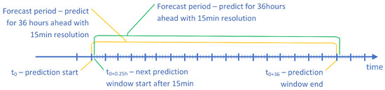
Figure 1. The scheme of the power generation system.

Additionally, the developed model should scale well such that it can be applied to a country-level to cover all wind farms.

In order to develop such a predictive model, we used two data sources. The first one was historical electric power generation recorded by the SCADA system installed on the power plant. The second component of the data was weather forecast data obtained from an institution delivering commercial weather forecasts. A detailed description of the weather forecast data is given in the following section.

The usage of two separate input data streams may result in synchronization problems. SCADA measurement data stream is received with a 15 min resolution, while numerical weather forecasts are provided four times a day through a public API. Therefore, to solve synchronization issues, we are building predictions every 15 min. Such an approach allows working on the latest available data chunks from both input streams.

3.1. Weather Forecast Data

The weather forecast is recalculated four times a day, every 6 h, and covers 42 h ahead with hourly resolution. It consists of two independent components: the wind field and the so-called “climate field”. All weather parameters are calculated on the grid with a 4 km bin, although the wind field and the climate field are shifted (as shown in Figure 2). In the wind-field forecast, each node of the grid consists of two components describing the wind speed: the N-S wind speed component and the E-W wind speed component, forecasted on the level of 100 m above the ground with hourly resolution. The climate-field consists of features such as pressure, relative humidity, temperature, etc., recorded 2 m above the ground.

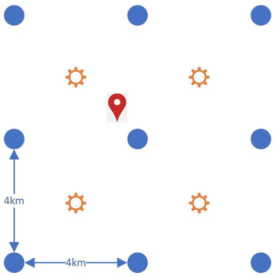
Figure 2. Weather forecast grid. Circles indicate wind-field nodes, suns indicate climate-field nodes, pin indicates wind farm location.

In order to reduce costs and speed-up calculations, only selected nodes were used from both of these fields. It is worth noting that the wind farms are usually distributed specially and their official geographical coordinates correspond to the service management facility, and not to the wind turbines. For example, the farms can spread along the hills—see Figure 3. Therefore, we gathered a wind field forecast for a 3 × 3 grid, centered on the node closest to the location of the power plant. The climate field is shifted, and the climate-graph nodes are centered in the middle of the square of the four wind field nodes as shown in Figure 2. Initially, we decided that for each wind farm, a 2 × 2 grid of the closest climate-field nodes will be considered. These parameters were identified as important, affecting the efficiency of the wind turbine, as discussed for example in [32,33]. Although our initial experiments indicated that these parameters do not influence the accuracy.

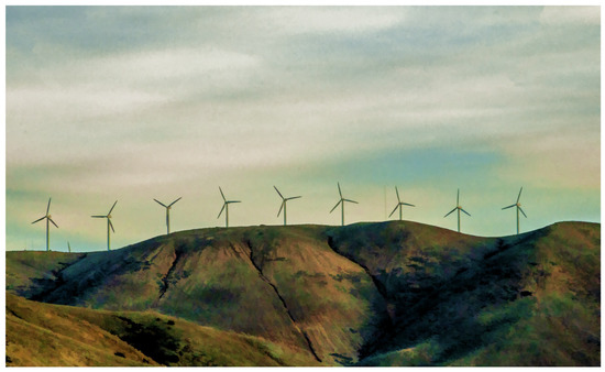
Figure 3. View on one of the wind farms. Source [34].

3.2. SCADA Data

Previously, we indicated that the second source of the data was SCADA. The obtained data covers real power generation from the wind farms together with the timestamp. The values of the generated power were recorded with a 15 min resolution. It is worth noting that the data used in the experiments did not include information on the number of operating turbines, only the total power generated power was available.

3.3. Dataset Description and Feature Generation

In the experiments, we used machine learning models for predicting power generation. They require the data to be formed as a $\{\mathbf{x},y\}$ pairs where $\mathbf{x}\in {\Re }^m$ is the input sample, or vector, consisting of m features, and $y\in \Re$ is the response feature that represents the desired output of the model. The goal of our predictive system was to forecast the power generation for 36 h ahead, with a 15 min resolution, and an update time of 15 min. In order to adapt the data obtained from the data sources described above to meet the requirements of the prediction model, every forecasted value was represented by a single sample. Therefore, for a single forecast start time, the model needs $4\left(\mathrm{times}\mathrm{per}\mathrm{hour}\right)·36\left(\mathrm{hours}\right)=144$ independent samples, one sample for every 15 min. Below, the experiments were conducted for a 1-year period, therefore the dataset consisted of $n=365\left(\mathrm{days}/\mathrm{year}\right)·24\left(\mathrm{hours}/\mathrm{day}\right)·4\left(\mathrm{times}/\mathrm{hour}\right)·144\left(\mathrm{number}\mathrm{of}\mathrm{samples}\mathrm{for}\mathrm{each}\mathrm{forecast}\right)\approx$ 5,000,000 samples.

As already indicated, the feature space of the input vector consists of two data sources, labeled data types, which were used to define the feature space of variables of $\mathbf{x}$. These were:

Type I

Based on the weather forecast (NWP—numerical weather predictions);

Type II

Autoregressive features describing the change of the power generation within the last 6 h before the forecast start;

Type III

Combined Type I and Type II.

The key attributes within Type I are the weather forecast data. Unfortunately, the resolution of these data was too low as they were recorded with hourly resolution and we needed to perform prediction with 15 min resolution. Therefore, the resolution of the wind speed features was increased by performing a spline-based interpolation.

Next, the two wind speed coordinates (N-S, and E-W) which are orthogonal were transformed into the wind speed and wind direction. Wind speed is directly related to power generation, so both wind speed and wind angle (direction) were added to the input data set. Additionally, the basic wind speed features were extended with the change of the wind speed and the change of the angle within two hours period before and two hours after the forecasted value. Here we could use the future wind change (two hours after the forecast) because we used the numerical weather forecast. Therefore, we can easily calculate not only the past changes in wind speed and wind direction but also the future changes in the wind. In fact, these features represent the gradients of the speed and gradients of the angle (the change calculated as $windSpeed\left(t\right)-windSpeed(t-2h)$ and $windSpeed(t+2h)-windSpeed\left(t\right)$).

Finally, the resultant wind speed and wind direction were calculated for every node of the wind field; similarly, we calculated wind speed and direction changes. This feature set was combined with the climate features which resulted in a wide range of features. Consequently, we considered a reduction of the feature space in order to simplify the model. To validate this assumption, we constructed 5 subsets of features that were evaluated in order to assess their prediction performance. These were

• Base features (CB)—a set that contains wind speed and wind direction taken from the closest NWP node;
• Base features with aggregates (CBAg)—besides (CB) it also includes mean temperature, relative humidity, and mean sea level pressure taken from the closest 4 “climate nodes”;
• Extended features with aggregates (RCBAg)—contains CBAg and also complete wind field from the surrounding 9 wind nodes, for both wind speed and wind direction;
• Extended features with aggregates plus (RCBAgP)—an extension of RCBAg; gradients were added for wind speed and wind direction, for 9 wind nodes, for two hours before and two hours after as described above;
• Extended features with aggregates plus spline interpolation (RCBAgPS)—all RCBAgP features plus new features being an approximation of the wind speed and wind direction into 15 min resolution.

Type II features were used similarly to the standard statistical autoregression models. Here, we used only the data describing historical power generation. The last recorded power generation historical data were transformed into a feature vector containing 8 values ${\mathbf{x}}_{\mathbf{G}}=\left[{\mathbf{x}}_{{\mathbf{G}}_{-}\mathbf{120}},{\mathbf{x}}_{{\mathbf{G}}_{-}\mathbf{105}},{\mathbf{x}}_{{\mathbf{G}}_{-}\mathbf{90}},{\mathbf{x}}_{{\mathbf{G}}_{-}\mathbf{75}},{\mathbf{x}}_{{\mathbf{G}}_{-}\mathbf{60}},{\mathbf{x}}_{{\mathbf{G}}_{-}\mathbf{45}},{\mathbf{x}}_{{\mathbf{G}}_{-}\mathbf{30}},{\mathbf{x}}_{{\mathbf{G}}_{-}\mathbf{15}}\right]$ where G indicates power generation and the lower index indicates time lag (in minutes). Next, the dataset was equipped with an additional feature representing the time passed from the forecast start time (the moment from which we start the calculations) until the forecast time (denoted as $x_R$), which is the time for which we want to obtain the forecast. This additional feature is important, because, as the $x_R$ increases, the ${\mathbf{x}}_{\mathbf{G}}$ degrades.

Type III features are a concatenation of Type I and Type II features, so that not only the wind forecast is available but also the autoregression data.

3.4. Experiment Setup

The experiment setup is presented in Figure 4. It starts by loading the raw data, this data set is then delivered to the feature generation operator, which returns a fully applicable dataset. Next, the dataset was delivered to the time series cross-validation procedure, which is based on linear sampling. We decided to use such a validation technique, and not a typical sliding window because power generation from windmills depends only on the weather conditions, therefore there is no chance for information leak. Moreover, from the training set, we removed a group of samples that share the same weather forecast (weather forecast is delivered every 6 h) within the training and testing set, so that each testing set has its own independent weather forecast.

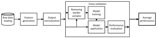
Figure 4. The scheme of the model evaluation process.

The procedure for the presented data was used to compare the performances of various machine learning prediction models including random forest [24], GBT [35], kNN [36], and fully connected neural network [37]. For each prediction model, we optimized its hyperparameters (see Table 1) using the internal cross-validation procedure. The internal cross-validation procedure, also called nested cross-validation, is an additional processing step to avoid overestimating the obtained model performance. As indicated by the authors of [38]: “In order to overcome the bias in performance evaluation, model selection should be viewed as an integral part of the model fitting procedure, and should be conducted independently in each trial in order to prevent selection bias and because it reflects best practice in operational use”, we also followed this procedure in order to assure the highest quality of the obtained results.

Table 1. The hyperparameters used for prediction model optimization.

Model	Param	Values
Random Forest	Trees	{50, 100, 300, 500}
	Depth	{2,5,7}
GBT	Trees	{50, 100, 200}
	Learning rate	{0.05, 0.1, 0.2}
MLP	Layers	{(10),(100),(100,10)}
	Iterations	{200,500}
kNN	k	{1,5,10,20,50,100}
	Weights	{uniform, distance}

Additionally, we analyzed soft ensemble models, where the model trained on type I data was combined with the model trained on type II dataset, and the model trained on type III dataset. The ensemble models were constructed in order to take advantage of the properties of the individual models, where each of the models has a different range of expertise. For example, the autoregression model (trained on type 2 dataset) has very good properties in the first several hours, while the model trained on the type 1 dataset has good properties for long-term prediction. These properties will be discussed in detail in the following section. In total, five prediction systems were constructed:

• Wind—Model trained on type I dataset;
• Autoreg.—Model trained on type II dataset;
• (Autoreg+Wind)—Model trained on type III dataset;
• Ens(Autoreg, (Autoreg+Wind)—Ensemble of two models, one trained on type 2 dataset and the other trained on type III dataset. Here, the Autoreg. model operated within the forecast range between 15 min and 3 h, while the (Autoreg Wind) model operated in the range of 2 h and 36 h forecast horizon, so in the range between 2 and 3 h these two models operated simultaneously. The final prediction was obtained by averaging the two results;
• Ensemble(all)—Ensemble of three models, these are Autoreg. model, (Autoreg + Wind) model and Wind model. Here, the Autoreg. model operated within the forecast range between 15 min and 3 h, the (Autoreg Wind) model operated in the range of 2 h and 18 h forecast, and the Wind model operated in range 8 until 36 h forecast; so the models often overlap in the range between 2 and 3 h and 8 until 18 h.

To evaluate the performance of the prediction models we used 3 indicators, that are Root Mean Square Error (RMSE), Mean Absolute Error (MAE), and Pearsons correlation R. In order to preserve the anonymity of the farms we used relative values, so the power generation variables were initially standardized to keep $mean=0$ and $std=1$. Therefore RMSE values equal 1 indicate a performance comparable to the naive model which always returns mean value of the training set, and $RMSE<1$ indicates improvement of the proposed prediction model.

After the initial model selection, we analyzed the learning curve for the selected model. This was particularly important because it allowed us to identify how much training data we would need to properly train the prediction models—as was previously mentioned the training set size was relatively large consisting of over $5·{10}^6$ samples. These experiments were evaluated for $n^{\prime }$ = [10,000, 20,000, 30,000, 40,000, 50,000, 60,000, 70,000, 100,000, 200,000, 500,000] samples taken randomly from the entire training set. Note that the constructed model should allow for easy retraining, and operation on a large of various wind farms.

Following this, we also evaluated the feature space, analyzing the influence of the feature group defined for Type I dataset. Here we evaluated the increasing subset of features so that we started from the simplest one containing only CB features, and evaluated more complex feature space up to RCBAgPS. All of the experiments were evaluated using the already mentioned cross-validation procedure.

3.5. Environment and Setup—Hardware and Software

The provided library is written in Python language, at least version 3.9. It requires a standard Python “numpy/scipy” stack as well as pandas library to be installed in a dedicated, separated environment (using “libenv” or any other tool to create isolated Python environments). For the ML models (random forest, kNN, GBT, NN, SVM) we used “scikit-learn” library. Our experiments were run on a server machine having 128 GB of RAM and 48 cores. Hardware requirements are set by the hyperparameters tuning and training procedures. For a single farm, training might be carried out in less than half an hour, while optimization time depends on the size of the hyperparameter grid search space. Prediction is preformed in a matter of seconds. The actual performance depends heavily on the final performance tuning phase which might be carried out in a future production phase.

4. Results

4.1. Model Selection

The first group of experiments was focused on the selection of the prediction model. For this issue, due to the computational complexity (each dataset consisted of over 5 million samples), we performed our analysis only on two wind farms, and on a single dataset type—the type 3 dataset. As indicated in the section describing the experiments, we compared 4 models: kNN, neural network, random forest, and GBT algorithm. Each of the models was optimized within each fold of the cross-validation procedure independently, using a grid search approach. In the evaluation, we limited the training set size to 50,000 samples (note that only the training set size was reduced, while the test size remained unchanged), which allowed us to make the evaluation process tractable. The obtained performances are shown in Table 2, which represent average performance over a 10-fold cross-validation test, and the reported execution time is the average training and prediction time over a single fold. Note that the training time includes model optimization time.

Table 2. Comparison of three different model performances on a single wind farm.

		RMSE	MAE	R	Training Time [s]	Prediction Time [s]
Farm A	Random Forest	0.575	0.414	0.755	1.891	0.287
	GBT	0.577	0.421	0.749	17.285	0.194
	kNN	0.594	0.440	0.735	0.007	58.031
	NeuralNet	0.576	0.419	0.750	50.688	0.172
Farm B	Random Forest	0.589	0.402	0.719	2.513	0.369
	GBT	0.597	0.415	0.711	13.908	0.064
	kNN	0.624	0.431	0.691	0.058	3.942
	NeuralNet	0.599	0.420	0.715	29.787	0.084

The obtained results indicate that the highest performance was obtained by the random forest prediction model. The results of random forest are comparable to the results obtained by the MLP neural network, although the training time of the neural network is significantly higher. In terms of prediction time, the neural network is comparable to the random forest, which is somewhat slower (note that the provided prediction time covers predicting of around 4.5 · 10⁶ samples). Similarly, there is a small difference in terms of error rate between random forest and GBT, although training time for GBT is significantly higher. This stems from the issue of parallelization, as in GBT, the trees are constructed sequentially so that the next tree can be constructed only when the previous tree is finished. The worst results were obtained by the kNN model. This model is also not applicable in terms of prediction time, which is very high. In view of the obtained results, the random forest is the preferred solution, which we kept for further evaluation. It has an additional advantage in easy parallelization, as well as feature importance analysis that avoids the black-box problem that appears in neural networks.

4.2. Learning Curve Analysis

Training time is one of the key issues facing our problem, where it is assumed that the prediction model will be retrained for each wind-farm after each week. It is required because the number of wind turbines is unknown during the execution of the model; therefore the addition or removal of any turbines may result in inaccurate results, although retraining helps to avoid this problem.

In light of this problem, the so-called learning curve was evaluated. The learning-curve displays the influence of the training set size on the prediction model performance. It allows limiting the training set size when the prediction performance stops increasing when enlarging the training set size. Similarly to the model selection, the results for only two farms are presented in Figure 5a,b.

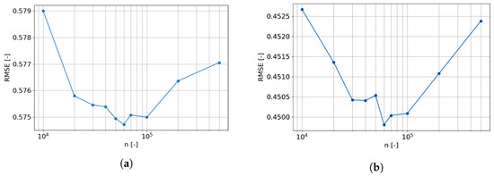
Figure 5. Learning curve. (a) Farm A. (b) Farm B.

The obtained results are surprising, as we observe that at the beginning the prediction error decreases, but at around $n^{\prime }$ = 50,000 samples, the error starts increasing. In other words, increasing the training set size result in reduced prediction performance. The analysis of the obtained decision trees within the random forest indicated, that the source of this phenomenon is the reduction of the diversity between the trees within the ensemble. In other words, for very large datasets, we observed that the decision trees started to converge to almost identical trees, therefore the prediction error started to increase. Finally, in the following calculations, we always sampled the training set and randomly selected $n^{\prime }$ = 50,000 samples.

4.3. Type I Features Set Analysis

As already mentioned, within this experiment five feature subsets (CB), (CBAg), (RCBAg), (RCBAgP) and (RCBAgPS) were evaluated. Those feature sets were ordered according to their increasing complexity—from the base ones (CB) up to the most complex (RCBAgPS), which require much higher computational cost to prepare. Therefore, we performed a ranking-based feature selection to find a compromise between computational costs and prediction performance by iteratively turning on an additional feature subset. These experiments were again only conducted on two example wind farms, and the obtained results are presented in Figure 6.

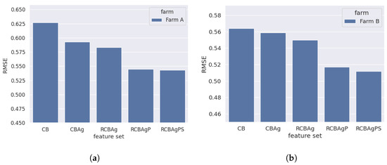
Figure 6. Feature selection algorithm results for both wind farms. For both farms, the biggest accuracy gain is obtained after including gradients of wind speed and direction into the feature set—RCBAgP. For both cases, we used the RMSE metric. (a) Farm A—feature selection procedure results. (b) Farm B—feature selection procedure results.

For both wind farms, the biggest increase in accuracy gain was observed for RCBAgP feature set—which contains wind speed and wind direction gradients. The results show, that climate variables and their aggregates, the CBAg feature set, do not improve prediction quality as much as might have been expected.

This phenomenon may result from the fact that the forecast of the climate variables (relative humidity, pressure, temperature) is given on the level of 2 m above the ground, which is only partially correlated with the values influencing wind turbines which are 90, or 120 m tall.

The remaining feature sets that were tested also did not lead to any significant lowering of the prediction error. Most notably, switching to the 15 min data resolution through the spline interpolation, as in the RCBAgPS feature set, did not increase accuracy significantly in comparison to the data in hourly resolution (RCBAgP set) while its computational cost was high. Thus, we have picked the RCBAgP feature set as a default one for further analysis.

4.4. Comparison of the Five Prediction Systems

The final experiments were focused on the analysis of the five prediction systems described in Section 3.4. Note, that these systems use the same type of prediction model, and differ in the feature space used for training the model as well as the construction of the ensemble for particular time ranges. A comparison of the obtained results for all of the evaluated wind farms is shown in Table 3.

Table 3. Obtained performances for each of the evaluated wind farms.

	Model	Autoreg	Wind	(Autoreg Wind)	Ens(Autoreg, (Autoreg Wind)	Ensemble(All)
Farm 1	RMSE	0.8538	0.6840	0.5883	0.5892	0.6384
	MAE	0.6424	0.4744	0.4008	0.4007	0.4376
	R	0.3700	0.6734	0.7189	0.7185	0.6978
Farm 2	RMSE	0.8521	0.6072	0.5746	0.5701	0.5821
	MAE	0.6947	0.4433	0.4140	0.4093	0.4218
	R	0.3996	0.7442	0.7550	0.7569	0.7557
Farm 3	RMSE	0.9048	0.5939	0.5526	0.5493	0.5698
	MAE	0.7151	0.4223	0.3914	0.3877	0.4034
	R	0.3868	0.7904	0.8150	0.8174	0.8036
Farm 4	RMSE	0.8916	0.5838	0.5817	0.5787	0.5801
	MAE	0.6891	0.3996	0.3965	0.3942	0.3954
	R	0.4016	0.7979	0.7978	0.7999	0.8003
Farm 5	RMSE	0.8776	0.4708	0.4714	0.4690	0.4686
	MAE	0.6830	0.3340	0.3336	0.3321	0.3315
	R	0.4060	0.8593	0.8581	0.8594	0.8596
Farm 6	RMSE	0.8714	0.4489	0.4495	0.4493	0.4478
	MAE	0.6836	0.3185	0.3189	0.3182	0.3168
	R	0.4265	0.8797	0.8791	0.8788	0.8799
Farm 7	RMSE	0.8493	0.5907	0.5713	0.5692	0.5768
	MAE	0.6660	0.4223	0.4032	0.4010	0.4090
	R	0.4067	0.7628	0.7616	0.7631	0.7661

These results indicate that on average the ensembles outperform the other systems; in particular, the best results were obtained by Ens(Autoreg, (Autoreg + Wind), which obtained the best results for 4 farms. The Ensemble(all) took the second place and obtained the best results for two farms but for those farms the difference between Ens(Autoreg, (Autoreg + Wind) is not significant, while for the Farm 2, Farm 3 and Farm 7 the Ens(Autoreg, (Autoreg + Wind) obtained significantly better results.

An extended analysis of the obtained performances is shown in Figure 7a,b. These plots show the relation between system performances in terms of the forecast period between 15 min and 36 h.

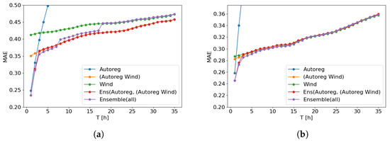
Figure 7. Model performance within the prediction range up to 36 h ahead. (a) Farm A. (b) Farm B.

These results indicate that within the first 2 h or 3 h, the lowest error rate is obtained by the models containing the autoregression features. As indicated by the Autoreg. system these type of features rapidly worsens, and after passing 3 h the system based on these-type of features becomes useless. For larger forecast horizons, except the ensembles, the combined autoregression and weather features embedded within (Autoreg + Wind) system start to obtain leading performance, which usually converges to the results obtained for the system based on the Wind features. Although, for Farm A we observe that the convergence is slow, while for Farm B it converges after 4 h. The ensemble systems allow to take benefit of individuals outperforming the basic systems, but only when the voting weights are appropriately tuned. Incorrectly tuned weights result in the system represented by the Ensemble(all) on Figure 7a, where the error rate jumps with a step-like function from the lower level to the upper level. In these particular experiments, we have tuned it manually, although it is possible to automatize this process; however, it is out of the scope of this article.

5. Conclusions

In this work, we studied a process of constituting and operationalizing a power generation prediction system from wind farms. Consequently, we analyzed data sources together with their processing and aggregation. We also compared various dataset construction types, where different data sources operated independently (type 1 and type 2) or together lead to type 3 dataset. On the obtained datasets various prediction models were compared by incorporating the construction of the ensembles where several models operate simultaneously in different forecast time ranges. Out of the conducted research and comparison, we can state that:

• Not always theoretically important features, which should affect power generation, are important in terms of forecasting mid-range values, this includes temperature, humidity and pressure;
• In short-term forecasting, the most influential is the autoregression data, which results from more consistent weather conditions; this level of error rate is unreachable using only the weather forecast data;
• When forecasting for more than a couple of hours, the weather forecast data starts to be more important, but usually, a model trained on combined autoregressive data and weather forecast works sufficiently;
• The best performance is obtained when several prediction models specializing in particular time ranges are combined together, leading to the ensemble model, although the aggregation process is very important and requires specific attention.

Out of the evaluated models, the most promising is the random forest, which achieved the highest performance; it has a reasonable training time and prediction time, as well as allowing for the analysis of all decisions taken.

References

- Biuletyn Miesieczny. Informacja statystyczna o enerrgii elektrycznej, Biuletyn miesięczny Nr 12 (336) Grudzień 2021. 2021. ISSN 1232-5457. Available online: https://www.are.waw.pl/component/phocadownload/category/19-informacja-statystyczna-o-energii-elektrycznej?download=143:informacja-statystyczna-o-energii-elektrycznej-nr-12-336-grudzien-2021 (accessed on 23 February 2022).
- GlobEnergia. Wiatraki-Rekord. 2021. Available online: https://globenergia.pl/wiatraki-wykrecily-rekord-produkcji-bezemisyjnej-energii-pomogla-nadia/ (accessed on 23 February 2022).
- Hanifi, S.; Liu, X.; Lin, Z.; Lotfian, S. A Critical Review of Wind Power Forecasting Methods—Past, Present and Future. Energies 2020, 13, 3764. [Google Scholar] [CrossRef]
- Tascikaraoglu, A.; Uzunoglu, M. A review of combined approaches for prediction of short-term wind speed and power. Renew. Sustain. Energy Rev. 2014, 34, 243–254. [Google Scholar] [CrossRef]
- Yousuf, M.U.; Al-Bahadly, I.; Avci, E. Current Perspective on the Accuracy of Deterministic Wind Speed and Power Forecasting. IEEE Access 2019, 7, 159547–159564. [Google Scholar] [CrossRef]
- Bochenek, B.; Jurasz, J.; Jaczewski, A.; Stachura, G.; Sekuła, P.; Strzyżewski, T.; Wdowikowski, M.; Figurski, M. Day-Ahead Wind Power Forecasting in Poland Based on Numerical Weather Prediction. Energies 2021, 14, 2164. [Google Scholar] [CrossRef]
- Yu, C.; Li, Y.; Bao, Y.; Tang, H.; Zhai, G. A novel framework for wind speed prediction based on recurrent neural networks and support vector machine. Energy Convers. Manag. 2018, 178, 137–145. [Google Scholar] [CrossRef]
- Shi, K.; Qiao, Y.; Zhao, W.; Wang, Q.; Wang, Q.; Liu, M.; Lu, Z. An improved random forest model of short-term wind-power forecasting to enhance accuracy, efficiency, and robustness. Wind Energy 2018, 21, 1383–1394. [Google Scholar] [CrossRef]
- Lahouar, A.; Slama, J.B.H. Hour-ahead wind power forecast based on random forests. Renew. Energy 2017, 109, 529–541. [Google Scholar] [CrossRef]
- Khosravi, A.; Machado, L.; Nunes, R. Time-series prediction of wind speed using machine learning algorithms: A case study Osorio wind farm, Brazil. Appl. Energy 2018, 224, 550–566. [Google Scholar] [CrossRef]
- Bilal, B.; Ndongo, M.; Adjallah, K.H.; Sava, A.; Kebe, C.M.; Ndiaye, P.A.; Sambou, V. Wind turbine power output prediction model design based on artificial neural networks and climatic spatiotemporal data. In Proceedings of the 2018 IEEE International Conference on Industrial Technology (ICIT), Lyon, France, 19–22 February 2018. [Google Scholar] [CrossRef]
- Zhang, J.; Yan, J.; Infield, D.; Liu, Y.; Lien, F.S. Short-term forecasting and uncertainty analysis of wind turbine power based on long short-term memory network and Gaussian mixture model. Appl. Energy 2019, 241, 229–244. [Google Scholar] [CrossRef]
- Wang, J.; Yang, W.; Du, P.; Niu, T. A novel hybrid forecasting system of wind speed based on a newly developed multi-objective sine cosine algorithm. Energy Convers. Manag. 2018, 163, 134–150. [Google Scholar] [CrossRef]
- Hong, Y.Y.; Rioflorido, C.L.P.P. A hybrid deep learning-based neural network for 24-h ahead wind power forecasting. Appl. Energy 2019, 250, 530–539. [Google Scholar] [CrossRef]
- Hatami, N.; Gavet, Y.; Debayle, J. Classification of time-series images using deep convolutional neural networks. In Proceedings of the Tenth International Conference on Machine Vision (ICMV 2017), Vienne, Austria, 13–15 November 2017; SPIE: Bellingham, WA, USA, 2018; Volume 10696, pp. 242–249. [Google Scholar]
- Chen, W.; Shi, K. A deep learning framework for time series classification using Relative Position Matrix and Convolutional Neural Network. Neurocomputing 2019, 359, 384–394. [Google Scholar] [CrossRef]
- Liu, T.; Huang, Z.; Tian, L.; Zhu, Y.; Wang, H.; Feng, S. Enhancing Wind Turbine Power Forecast via Convolutional Neural Network. Electronics 2021, 10, 261. [Google Scholar] [CrossRef]
- Yu, Y.; Si, X.; Hu, C.; Zhang, J. A review of recurrent neural networks: LSTM cells and network architectures. Neural Comput. 2019, 31, 1235–1270. [Google Scholar] [CrossRef] [PubMed]
- Dudek, G.; Pełka, P.; Smyl, S. A hybrid residual dilated LSTM and exponential smoothing model for midterm electric load forecasting. IEEE Trans. Neural Netw. Learn. Syst. 2021, 33, 2879–2891. [Google Scholar] [CrossRef] [PubMed]
- Delgado, I.; Fahim, M. Wind turbine data analysis and LSTM-based prediction in SCADA system. Energies 2020, 14, 125. [Google Scholar] [CrossRef]
- Li, S. Wind power prediction using recurrent multilayer perceptron neural networks. In Proceedings of the 2003 IEEE Power Engineering Society General Meeting (IEEE Cat. No. 03CH37491), Toronto, ON, Canada, 13–17 July 2003; IEEE: New York, NY, USA, 2003; Volume 4, pp. 2325–2330. [Google Scholar]
- Zendehboudi, A.; Baseer, M.A.; Saidur, R. Application of support vector machine models for forecasting solar and wind energy resources: A review. J. Clean. Prod. 2018, 199, 272–285. [Google Scholar] [CrossRef]
- Chang, C.C.; Lin, C.J. LIBSVM: A library for support vector machines. ACM Trans. Intell. Syst. Technol. (TIST) 2011, 2, 1–27. [Google Scholar] [CrossRef]
- Breiman, L. Random Forests. Mach.-Mediat. Learn. 2001, 45, 5–32. [Google Scholar] [CrossRef]
- Dudek, G. A Comprehensive Study of Random Forest for Short-Term Load Forecasting. Energies 2022, 15, 7547. [Google Scholar] [CrossRef]
- Iannace, G.; Ciaburro, G.; Trematerra, A. Wind turbine noise prediction using random forest regression. Machines 2019, 7, 69. [Google Scholar] [CrossRef]
- Schapire, R.E. Explaining adaboost. In Empirical Inference; Springer: New York, NY, USA, 2013; pp. 37–52. [Google Scholar]
- Chen, T.; He, T.; Benesty, M.; Khotilovich, V.; Tang, Y.; Cho, H.; Chen, K.; Mitchell, R.; Cano, I.; Zhou, T. Xgboost: Extreme Gradient Boosting. R Package Version 0.4-2 2015, 1, 1–4. [Google Scholar]
- Ke, G.; Meng, Q.; Finley, T.; Wang, T.; Chen, W.; Ma, W.; Ye, Q.; Liu, T.Y. Lightgbm: A highly efficient gradient boosting decision tree. Adv. Neural Inf. Process. Syst. 2017, 30, 52. [Google Scholar]
- Zheng, H.; Wu, Y. A xgboost model with weather similarity analysis and feature engineering for short-term wind power forecasting. Appl. Sci. 2019, 9, 3019. [Google Scholar] [CrossRef]
- Cai, L.; Gu, J.; Ma, J.; Jin, Z. Probabilistic wind power forecasting approach via instance-based transfer learning embedded gradient boosting decision trees. Energies 2019, 12, 159. [Google Scholar] [CrossRef]
- Pang, C.; Yu, J.; Liu, Y. Correlation analysis of factors affecting wind power based on machine learning and Shapley value. IET Energy Syst. Integr. 2021, 3, 227–237. [Google Scholar] [CrossRef]
- Baskut, O.; Ozgener, O.; Ozgener, L. Effects of meteorological variables on exergetic efficiency of wind turbine power plants. Renew. Sustain. Energy Rev. 2010, 14, 3237–3241. [Google Scholar] [CrossRef]
- Wind Turbines Free Stock Photo—Public Domain Pictures. Available online: https://www.publicdomainpictures.net/en/view-image.php?image=270398&picture=wind-turbines (accessed on 22 December 2022).
- Natekin, A.; Knoll, A. Gradient boosting machines, a tutorial. Front. Neurorobot. 2013, 7, 21. [Google Scholar] [CrossRef]
- de Souza Junior, A.H.; Corona, F.; Barreto, G.A.; Miche, Y.; Lendasse, A. Minimal learning machine: A novel supervised distance-based approach for regression and classification. Neurocomputing 2015, 164, 34–44. [Google Scholar] [CrossRef]
- Gurney, K. An Introduction to Neural Networks; CRC Press: Boca Raton, FL, USA, 2018. [Google Scholar]
- Brownlee, J. Nested Cross-Validation for Machine Learning with Python. Machine Learning Mastery. 2020. Available online: https://machinelearningmastery.com/nested-cross-validation-for-machine-learning-with-python (accessed on 23 February 2023).
Disclaimer/Publisher’s Note: The statements, opinions and data contained in all publications are solely those of the individual author(s) and contributor(s) and not of MDPI and/or the editor(s). MDPI and/or the editor(s) disclaim responsibility for any injury to people or property resulting from any ideas, methods, instructions or products referred to in the content. |
© 2023 by the authors. Licensee MDPI, Basel, Switzerland. This article is an open access article distributed under the terms and conditions of the Creative Commons Attribution (CC BY) license (https://creativecommons.org/licenses/by/4.0/).