Operating Hydrogen-Based Energy Storage Systems in Wind Farms for Smooth Power Injection: A Penalty Fees Aware Model Predictive Control

Abstract

Smooth power injection is one of the possible services that modern wind farms could provide in the not-so-far future, for which energy storage is required. Indeed, this is one among the three possible operations identified by the International Energy Agency (IEA)-Hydrogen Implementing Agreement (HIA) within the Task 24 final report, that may promote their integration into the main grid, in particular when paired to hydrogen-based energy storages. In general, energy storage can mitigate the inherent unpredictability of wind generation, providing that they are deployed with appropriate control algorithms. On the contrary, in the case of no storage, wind farm operations would be strongly affected, as well as their economic performances since the penalty fees wind farm owners/operators incur in case of mismatches between the contracted power and that actually delivered. This paper proposes a Model Predictive Control (MPC) algorithm that operates a Hydrogen-based Energy Storage System (HESS), consisting of one electrolyzer, one fuel cell and one tank, paired to a wind farm committed to smooth power injection into the grid. The MPC relies on Mixed-Logic Dynamic (MLD) models of the electrolyzer and the fuel cell in order to leverage their advanced features and handles appropriate cost functions in order to account for the operating costs, the potential value of hydrogen as a fuel and the penalty fee mechanism that may negatively affect the expected profits generated by the injection of smooth power. Numerical simulations are conducted by considering wind generation profiles from a real wind farm in the center-south of Italy and spot prices according to the corresponding market zone. The results show the impact of each cost term on the performances of the controller and how they can be effectively combined in order to achieve some reasonable trade-off. In particular, it is highlighted that a static choice of the corresponding weights can lead to not very effective handling of the effects given by the combination of the system conditions with the various exogenous’, while a dynamic choice may suit the purpose instead. Moreover, the simulations show that the developed models and the set-up mathematical program can be fruitfully leveraged for inferring indications on the devices’ sizing.

1. Introduction

In 2013, the IEA released the final report of Task 24 operating under the HIA and carried out between spring 2007 and autumn 2011 [1]. The purpose was “to provide an overview for technologies which have a direct influence on development and implementation of systems integrating wind energy with hydrogen production […]”, or, in other words, wind-hydrogen systems. The report categorizes wind-hydrogen systems (i.e., wind farms paired to HESSs) with respect to their main purpose and in terms of relevant sizes, identifying three categories. Systems under the “Electricity-storage” category target power smoothing against fluctuations in wind power by “[…] producing hydrogen at times of surplus power production and re-electrifying it during periods of underproduction. Such devices could facilitate wind power integration on a large scale, independent of support from fossil-fuel power stations.” Thus, multiple balancing services can be provided to the grid addressing different timescales: from the shorter, where power balancing for voltage and frequency stability is addressed, to the mid-range, where energy balancing is addressed, to the larger, where the grid is supported in order to mitigate temporary bottlenecks.

This is also reflected in the scientific literature on power smoothing in wind farms, where even larger timescale ranges are addressed. For instance, in Zhao et al. [2] the authors investigate how the inertial energy of the turbines can be optimized in order to provide power smoothing across timescales of seconds, while timescales of the order of tens of seconds are, instead, addressed by Lyu et al. [3] where two strategies are developed and presented: firstly, power smoothing is targeted by simultaneous operations of the dc-link voltage control, the rotor speed control and the pitch angle control; then, a hierarchical arrangement is also proposed, which suitably and dynamically combines the three individual control schemes during the operations across timescales of the order of hundreds of seconds. Moving forward to timescales of the order of minutes, for example Lyu et al. [4] develops an automatic generation control for power smoothing which is set in response to the actual grid needs. At this point, the literature jumps to timescales of the order of hours, targeting, e.g., market participation/demand response programs [5,6,7] but without power smoothing, which instead is investigated in Abdelghany et al. [8], where an MPC-based strategy is developed featuring a two-step sequential optimization: firstly, a function of the previous output power variations, such that the new decided value does not lie too far from previous ones, is minimized; secondly, other costs are minimized, such as, e.g., a reference tracking cost, and, among the others, a similar function used in the first step is constrained so as not to exceed the previously optimal computed value. In this paper, we investigate a scenario similar to [8], which shares some of the authors of this paper; however, later, the differences will be highlighted in order to identify the major advancements and novelties beyond the state of the art.

Many other aspects concerning power smoothing in wind farms are also addressed by the literature. For instance, in Koiwa et al. [9] a control approach for power smoothing is proposed such that the required rated power of the used energy storage system can be reduced against what would be a typical design. In Yang et al. [10], the power smoothing that can be inherently achieved by clusters of wind turbines at the point of common coupling, is investigated against many parameters, such as different timescales and sampling intervals, wind speed, number of wind turbines, etc. In general, power smoothing in renewable energy plants is a very wide topic. The interested reader can refer to Barra et al. [11], where wind farms are specifically addressed, to Lamsal et al. [12], which also addresses photovoltaic generation and the references therein for comprehensive reviews.

Another interesting aspect relates to the used energy storage system. As an example, in Zhai et al. [13] the authors investigate the effectiveness of superconducting magnetic energy storage for power smoothing, while in Yang and Jin [14] the authors target output power smoothing with superconducting energy storage along with the additional aspects of low voltage ride-through capacity and power oscillations under asymmetrical faults; in Wang et al. [15], a dual battery energy storage system is considered in order to reduce the number of charging/discharging per battery, thus improving each battery’s lifetime and the energy storage system economy in general. A good review of the literature targeting different kinds of energy storage systems (e.g., battery-, supercap-, flywheel-based, etc.), can be found always in Barra et al. [11], while aspects related to the performances of battery-based energy storage systems, with the aim of power smoothing in wind farms, are investigated in Sattar et al. [16]. Finally, hybrid configurations are also addressed [17,18]. Of course, the adopted energy storage systems interplay also with the possible timescales where they can be effectively operated, as show by [13,14] where timescales of the order of fractions of seconds and seconds are targeted, respectively.

Unfortunately, the above-mentioned papers do not address the case of HESSs. In this direction, some papers can be found roughly dating back to the first decade of 2000 [19,20,21,22]. Then, the topic shows a lesser relevance in the second decade while gaining a slightly increasing momentum in the current one, for instance, addressing hybrid storage systems hydrogen- and battery-based [23], hydrogen- and superconducting magnet-based [24], or coordinating a kinetic energy and a virtual discharge control [25].

In general, except for Abdelghany et al. [8], to the best of the authors’ knowledge, the literature seems to not address exactly the use-case energy-storage as identified by the IEA-HIA in the final report of Task 24. In particular, this paper shares some similarities with Abdelghany et al. [8]:

• The scenario, i.e., a wind-hydrogen system targeting the use-case energy-storage as per the IEA-HIA Task 24 final report;
• The MLD modeling for including devices’ dynamics depending on logical conditions;
• The MPC-based approach;
• The minimization of the devices’ operating costs.

However, many differences exist and additional aspects are considered:

• Accounting for the power smoothing based on tracking a smooth profile contracted with the Transmission System Operator (TSO);
• Accounting for the participation to the spot market, which is competing with the aim of providing smooth power to the grid, since, for instance, the controller is also pushed not to electrolyze in case of both wind production and spot market prices peak;
• Accounting for the penalties that the wind farm owner/operator incurs in case the delivered power is below a threshold against what contracted;
• Accounting for the inherent hydrogen value, which is competing with the aim of providing smooth power to the grid, yet it is appealing for the wind farm owner/operator for leveraging hydrogen production for other purposes aside from the main one (i.e., power smoothing);
• Simpler devices’ models based on practical considerations about their functioning and cost impacts on the optimal operations;
• Simpler control architecture with no sequential optimization;
• Simulations with real data from a wind farm in the center-south of Italy and real spot prices.

Finally, also fee-aware mechanisms seem not addressed by the literature, at least in the case of wind farms connected to the grid, to the best of the authors’ knowledge.

The rest of the paper is organized as follows: In Section 2 the used mathematical frameworks and the development of the algorithms are presented, while Section 3 reports the simulation scenarios and corresponding results. Further, there we also provide an impact analysis of each cost term considered and possible choices of the corresponding weights. Section 4 concludes the paper.

2. Materials and Methods

The core tools used for the proposed investigation are the MLD framework for modeling and the MPC scheme for control.

2.1. MLD Framework

Systems governed by physical laws, logic rules and constraints are known as MLD systems and can be modeled as dynamic equations subject to linear inequalities where real and integer/Boolean variables appear [26], which establishes the so-called MLD framework. The power of the framework is that, for instance, qualitative facts can also be rephrased into logic rules and thus accounted for via inequalities in, e.g., a possible mathematical program implemented and solved via an MPC scheme for control purposes, as happens in this paper.

The underlying machinery can be easily understood with a few examples, while for a thorough presentation the reader is referred to Bemporad and Morari [26] and the references therein. An important ingredient is the link that can be established between a function, say f, and an indicator variable, say $\delta$, such that, e.g., $f>0$ implies $\delta =1$. The indicator variable can be a logic variable when systems with dynamics depending also on logic conditions are targeted. In other terms, an important ingredient is how logical statements can be translated into mathematical inequalities. For instance, we consider the statement $[f>0]\to [\delta =1]$, where the brackets indicate the sentence resulting by the articulation of the mathematical condition they enclose, i.e., $[f>0]$ stands for “the function f is positive” and $[f>0]\to [\delta =1]$ indicates the compound statement “the function f is positive implies the indicator variable $\delta$ is 1”. Thus, it is easy to check that [27]

$$[f>0]\to [\delta =1]\mathrm{is}\mathrm{equivalent}\mathrm{to}f\le \left(\max f\right)\delta .$$

(1)

Indeed, if $f>0$, the only way for the mathematical inequality on the right of (1) to be true is that $\delta =1$, while, if $f\le 0$, the statement on the left of (1) does not enable any conclusion about $\delta$ and the same holds for the inequality on the right. We stress that, in (1), $\max f$ is necessary since the inequality must hold for any value f can take, but any other number greater than $\max f$ is sufficient. Indeed, sometimes it is easier to find an overestimate of $\max f$, though this may imply higher computational burdens for an optimizer, e.g., in case the models are used in a mathematical program that is subsequently solved numerically.

Now, in the paper we will also often use $[f\le 0]\to [\delta =1]$ which can be easily worked out by rephrasing it similarly to (1). Firstly, we notice that $[f\le 0]\to [\delta =1]$ can be rephrased as $[f<ϵ]\to [\delta =1]$, where $ϵ>0$ is a tolerance such that zero is accounted for and inequality is assumed satisfied. This comes also in handy when the equations are implemented on a digital computer such that the tolerance can be set to the machine’s precision. Then, by another small rephrasing, we obtain $[f-ϵ<0]\to [\delta =1]$, following $[-f+ϵ>0]\to [\delta =1]$. Thus, by comparison with (1), we achieve

$$[f\le 0]\to [\delta =1]\mathrm{is}\mathrm{equivalent}\mathrm{to}f\ge ϵ+(\min f-ϵ)\delta ,$$

(2)

since $\max -f=-\min f$.

2.2. MPC Schemes

MPC schemes are widely adopted control schemes where, in a typical and simple implementation, a control problem is cast at discrete-time $\mathrm{k}$, such that, at each time step, optimal commands $u_{\mathrm{k}}^{*}$ are provided to the target plant via the optimization of a cost function subject to some constraints, see Figure 1. The optimization is carried out across a (prediction) horizon of duration $\mathrm{N}$ ahead in the future, with a set of constraints including also the plant dynamics, and resulting in $\mathrm{N}$ optimal commands, say $u_{\mathrm{k}}^{*},\dots ,u_{\mathrm{k}+\mathrm{N}-1}^{*}$. However, only the first one is applied while the others are discarded, because the optimization is re-triggered at $\mathrm{k}+1$, such that the new state of the plant, determined by the implementation of $u_{\mathrm{k}}^{*}$, is considered and updated exogenous conditions are handled as well.

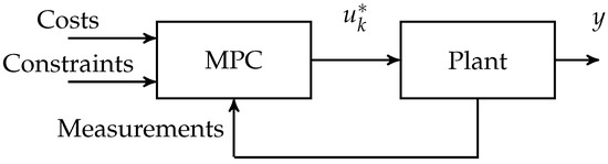
Figure 1. A simple MPC scheme.

Of course, as already said, what is explained refers to one of the many possible implementations of MPC that can be found in the literature. Yet, this suffices for the exposition of the results that are presented in this paper.

2.3. Assumptions and Notation

Throughout the paper, the following assumptions and notations will be used: α, β ∈ {STB,ON} are two generic indices, where STB,ON are the admissible logic states for a device’s corresponding automaton; sometimes α and β are used in conjunction and in this case we agree that α ≠ β; logic variables are ${\delta }^{\mathsf{\alpha }},{\sigma }_{\mathsf{\beta }}^{\mathsf{\alpha }},{\zeta }_{\le }^{\mathsf{\alpha }},{\zeta }_{\ge }^{\mathsf{\alpha }}\in \{0,1\}$ and mixed-logic variables are ys with some superscript, e.g., $y^{\mathsf{\alpha }}$ given by the product of $p{\delta }^{\mathsf{\alpha }}$, with $p\in {\mathbb{R}}^{+}$; small slanted fonts are used to indicate time-varying quantities at current discrete-time $\mathrm{k}$; ${\mathrm{T}}_{\mathrm{s}}$ and $\mathrm{N}$ are the sampling time and the control horizon, respectively, and the notation ${\left(\phantom{x}\right)}^{+}$ is used to indicate a time-varying variable at the next time step; sometimes the subscripts ${}_{\mathrm{e}}$ and ${}_{\mathrm{f}}$ will be used to highlight that a quantity refers to the “$\mathrm{e}$”lectrolyzer or to the “$\mathrm{f}$”uel cell, respectively. Finally, $\mathbf{1}$ and $\mathbf{0}$ indicate column vectors of suitable dimensions with unitary and null entries, respectively, and bold letters indicate vectors that, in this paper, gather samples of the corresponding scalar time-varying quantity, increasingly from the current time, across the horizon $\mathrm{N}$, e.g., ${\mathbf{\delta }}^{\mathsf{\alpha }}=\left[\begin{array}{c}{\delta }^{\mathsf{\alpha }}\left(\mathrm{k}\right)\dots {\delta }^{\mathsf{\alpha }}(\mathrm{k}+\mathrm{N}-1)\end{array}\right]$ and ${({\mathbf{\delta }}^{\mathsf{\alpha }})}^{+}=\left[\begin{array}{c}{\delta }^{\mathsf{\alpha }}(\mathrm{k}+1)\dots {\delta }^{\mathsf{\alpha }}(\mathrm{k}+\mathrm{N})\end{array}\right]$.

For the reader’s convenience, in Table 1 the list of symbols used throughout the paper is also reported. There, we followed the rule that, for each reported symbol class, Greek letters go first.

Table 1. List of symbols.

Variables
${\delta }^{\mathsf{\alpha }}$	Logic variable of a generic state $\mathsf{\alpha }$
${\delta }^{\mathrm{fee}}$	Logic variable indicating the activation of a penalty fee
${\sigma }_{\mathsf{\beta }}^{\mathsf{\alpha }}$	Logic variable of two generic states $\mathsf{\alpha }$ and $\mathsf{\beta }$
$y^{\mathsf{\alpha }}$	Mixed variable of a generic state $\mathsf{\alpha }$
$y^{\mathrm{fee}}$	Mixed variable involved in the activation of a penalty fee
${\zeta }_{\le }^{\mathsf{\alpha }}$, ${\zeta }_{\ge }^{\mathsf{\alpha }}$	Logic (slack) variables of a generic state $\mathsf{\alpha }$
$\mathit{loh}$	Level of hydrogen in the tank
e	Price profile contracted by the wind farm operator/
	owner with the Transmission System Operator (TSO)
p	A generic device’s power
$p_{\mathrm{grid}}$	Power delivered to the grid
$p_{\mathrm{ref}}$	Reference power profile to track
$p_{\mathrm{w}}$	Power profile by wind generation
s	Energy prices in the spot market
Cost terms
$c_{\mathrm{N}}$	Total costs across a horizon $\mathrm{N}$
$c^{\sigma }$ ($c_{\mathrm{N}}^{\sigma }$)	Cost term related to state switchings of a generic device (across a horizon $\mathrm{N}$)
$c^{\mathit{loh}}$ ($c_{\mathrm{N}}^{\mathit{loh}}$)	Cost term related to the level of hydrogen in the tank (across a horizon $\mathrm{N}$)
$c^{\mathrm{OP}}$ ($c_{\mathrm{N}}^{\mathrm{OP}}$)	Cost term related to the operations of a generic device (across a horizon $\mathrm{N}$)
$c^{p_{\mathrm{grid}}}$ ($c_{\mathrm{N}}^{p_{\mathrm{grid}}}$)	Cost term related to the tracking error of a power reference (across a horizon $\mathrm{N}$)
$c^{\mathrm{fee}}$ ($c_{\mathrm{N}}^{\mathrm{fee}}$)	Cost term related to the activation of a penalty fee (across a horizon $\mathrm{N}$)
$d_{\mathrm{N}}$	Total costs across a horizon $\mathrm{N}$ of a generic device
Labels
STB, ON	Names of logic states of a generic device’s automaton
Parameters
${\mathsf{ϵ}}^{\mathrm{fee}}$	Small tolerance
${\mathsf{\Pi }}_{\mathrm{e}}$	Productivity of the electrolyzer
${\mathsf{\Pi }}_{\mathrm{f}}$	Productivity of the fuel cell
${\mathrm{C}}_{\mathrm{H}}$	Cost of hydrogen
${\mathrm{C}}_{\mathrm{STB}}^{\mathrm{ON}}$	Cost for a generic device to switch from $\mathrm{STB}$ to $\mathrm{ON}$
${\mathrm{C}}_{\mathrm{ON}}^{\mathrm{STB}}$	Cost for a generic device to switch from $\mathrm{ON}$ to $\mathrm{STB}$
${\mathrm{C}}^{\mathrm{s}}$	Part of earnings paid by the wind farm operator/owner to a third party company
${\mathcal{D}}_{\mathrm{N}}$	Set of a generic device’s decision variables across a horizon $\mathrm{N}$
${\mathrm{H}}^{\max }$	Maximum rated amount of hydrogen in the tank
${\mathrm{LOH}}^{\max }$	Maximum level of hydrogen in the tank
${\mathrm{LOH}}^{\min }$	Minimum level of hydrogen in the tank
${\mathrm{M}}^{\mathsf{\alpha },\max }$	Upper-bound estimate of $p-{\mathrm{P}}^{\mathsf{\alpha },\max }$
${\mathrm{M}}^{\mathsf{\alpha },\min }$	Upper-bound estimate of $p-{\mathrm{P}}^{\mathsf{\alpha },\min }$
${\mathrm{M}}^{\mathrm{fee}}$	Upper-bound estimate of $p_{\mathrm{grid}}-p_{\mathrm{ref}}+\Delta {\mathrm{P}}^{\mathrm{fee}}$
${\mathrm{m}}^{\mathrm{fee}}$	Lower-bound estimate of $p_{\mathrm{grid}}-p_{\mathrm{ref}}+\Delta {\mathrm{P}}^{\mathrm{fee}}$
${\mathrm{M}}^{y^{\mathsf{\alpha }}}$	Upper-bound estimate of $y^{\mathsf{\alpha }}$
${\mathrm{m}}^{y^{\mathsf{\alpha }}}$	Lower-bound estimate of $y^{\mathsf{\alpha }}$
$\mathrm{N}$	Horizon
${\mathrm{P}}^{\mathsf{\alpha },\max }$	A generic device’s maximum power when in state $\mathsf{\alpha }$
${\mathrm{P}}^{\mathsf{\alpha },\min }$	A generic device’s minimum power when in state $\mathsf{\alpha }$
${\mathrm{P}}_{\mathrm{e}}^{\mathrm{STB}}$	Rated power of the electrolyzer in stand-by
${\mathrm{P}}_{\mathrm{f}}^{\mathrm{STB}}$	Rated power of the fuel cell in stand-by
${\mathrm{P}}_{\mathrm{e}}^{\max }$	Maximum rated power of the electrolyzer in on
${\mathrm{P}}_{\mathrm{e}}^{\min }$	Minimum rated power of the electrolyzer in on
${\mathrm{P}}_{\mathrm{f}}^{\max }$	Maximum rated power of the fuel cell in on
${\mathrm{P}}_{\mathrm{f}}^{\min }$	Minimum rated power of the fuel in on
${\mathrm{T}}_{\mathrm{s}}$	Sampling time
${\mathrm{W}}^{\sigma }$	Weight related to the cost term $c^{\sigma }$ ($c_{\mathrm{N}}^{\sigma }$)
${\mathrm{W}}^{\mathit{loh}}$	Weight related to the cost term $c^{\mathit{loh}}$ ($c_{\mathrm{N}}^{\mathit{loh}}$)
${\mathrm{W}}^{\mathrm{fee}}$	Weight related to the cost term $c^{\mathrm{fee}}$ ($c_{\mathrm{N}}^{\mathrm{fee}}$)
${\mathrm{W}}^{\mathrm{OP}}$	Weight related to the cost term $c^{\mathrm{OP}}$ ($c_{\mathrm{N}}^{\mathrm{OP}}$)
${\mathrm{W}}^{p_{\mathrm{grid}}}$	Weight related to the cost term $c^p$ ($c_{\mathrm{N}}^p$)

2.4. Description of the Scenario

Figure 2 depicts the scenario addressed, which is similar to that of [8], however with significant differences about the technological assumptions on the electrolyzer and the fuel cell, among the others.

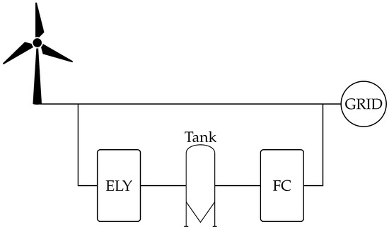
Figure 2. Simplified sketch of the addressed scenario. ELY stands for “electrolyzer” and FC stands for “fuel cell”.

Technology Driven Assumptions

• Stand-by requires very low power, both for the electrolyzer and the fuel cell, that would otherwise need a very long off-duty period in order to be economically convenient to opt for off operations. Therefore, in our mathematical modeling, we do not consider a device can be switched off; in turn, this also implies that cold starts are subsequently not accounted for.
• The sampling time addressed by the controller (order of tens of minutes) is much greater than the timescale across which warm starts take place (order of seconds), which, therefore, are not accounted for.
• The devices have good time-response performance so that some typical limitations such as, e.g., ramp limits, are ineffective at the considered sampling times.

These assumptions and corresponding consequences are beneficial because they enable the formulation of simpler Mixed-Integer Linear (MIL) programs equipped with a reduced number of constraints to be fulfilled, e.g., with respect to [8].

2.5. Devices’ Logic Models

A device functioning is described by the conditions

$$p-{\mathrm{P}}^{\mathsf{\alpha },\min }\ge 0,p-{\mathrm{P}}^{\mathsf{\alpha },\max }\le 0\iff {\delta }^{\mathsf{\alpha }}=1,$$

(3)

where ${\delta }^{\mathsf{\alpha }}$, which is 1 if state $\mathsf{\alpha }$ is $\mathrm{TRUE}$, 0 otherwise, is a logic function of the state $\mathsf{\alpha }$, and $[{\mathrm{P}}^{\mathsf{\alpha },\min },{\mathrm{P}}^{\mathsf{\alpha },\max }]$ identifies a power range which is relevant for that particular state α. Figure 3 depicts a generic automaton such that the logic behavior of each device will be modeled via one corresponding instance. The picture also reports the transitions $\sigma$s among the states, that will be defined later and used to introduce corresponding switching costs.

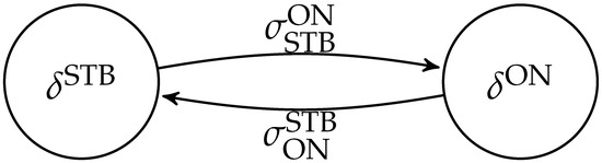
Figure 3. Two-state automaton for a generic device. The electrolyzer and the fuel cell operations are modeled according to two corresponding different instances.

2.5.1. MLD Modeling

Equation (3) has to be recast so that it can be easily handled by numerical optimizers. Indeed, by applying the MLD modeling [26] directly to (3), the achieved inequalities would force p to take values within not compatible ranges when ${\delta }^{\mathsf{\alpha }}=0$, thus resulting in an unfeasible inequality set for the optimizer. Instead, a feasible inequality set can be achieved via the adoption of suitable (auxiliary/slack) logical variables zs that encode only the right-to-left implication in (3). In addition, for each inequality $p-{\mathrm{P}}^{\mathsf{\alpha },\min }\ge 0,p-{\mathrm{P}}^{\mathsf{\alpha },\max }\le 0$, a corresponding set of logical variables has to be used, i.e., ${\zeta }_{\ge }^{\mathsf{\alpha }}$ and ${\zeta }_{\le }^{\mathsf{\alpha }}$, respectively.

Thus,

$$[{\zeta }_{\ge }^{\mathsf{\alpha }}=1]\to [p-{\mathrm{P}}^{\mathsf{\alpha },\min }\ge 0]\wedge [{\zeta }_{\ge }^{\mathsf{\alpha }}=0]\to [p-{\mathrm{P}}^{\mathsf{\alpha },\min }<0],$$

(4)

are recast as

$$\begin{array}{cc}\hfill -(p-{\mathrm{P}}^{\mathsf{\alpha },\min }) \le & {\mathrm{M}}^{\mathsf{\alpha },\min }(1-{\zeta }_{\ge }^{\mathsf{\alpha }}),\hfill \end{array}$$

(5a)

$$\begin{array}{cc}\hfill p-{\mathrm{P}}^{\mathsf{\alpha },\min } \le & {\mathrm{M}}^{\mathsf{\alpha },\min }{\zeta }_{\ge }^{\mathsf{\alpha }}, \hfill \end{array}$$

(5b)

respectively, and

$$[{\zeta }_{\le }^{\mathsf{\alpha }}=1]\to [p-{\mathrm{P}}^{\mathsf{\alpha },\max }\le 0]\wedge [{\zeta }_{\le }^{\mathsf{\alpha }}=0]\to [p-{\mathrm{P}}^{\mathsf{\alpha },\max }>0],$$

(6)

are recast as

$$\begin{array}{cc}\hfill p-{\mathrm{P}}^{\mathsf{\alpha },\max } \le & {\mathrm{M}}^{\mathsf{\alpha },\max }(1-{\zeta }_{\le }^{\mathsf{\alpha }}),\hfill \end{array}$$

(7a)

$$\begin{array}{cc}\hfill -(p-{\mathrm{P}}^{\mathsf{\alpha },\max }) \le & {\mathrm{M}}^{\mathsf{\alpha },\max }{\zeta }_{\le }^{\mathsf{\alpha }},\hfill \end{array}$$

(7b)

respectively, where ${\mathrm{M}}^{\mathsf{\alpha },\min }\ge \max (p-{\mathrm{P}}^{\mathsf{\alpha },\min })$ and ${\mathrm{M}}^{\mathsf{\alpha },\max }\ge \max (p-{\mathrm{P}}^{\mathsf{\alpha },\max })$.

Then, it is necessary to establish a link among ${\delta }^{\mathsf{\alpha }}$s and ${\zeta }_{\ge }^{\mathsf{\alpha }}$s, ${\zeta }_{\le }^{\mathsf{\alpha }}$s, such that when ${\delta }^{\mathsf{\alpha }}=1$, then $p\in [{\mathrm{P}}^{\mathsf{\alpha },\min },{\mathrm{P}}^{\mathsf{\alpha },\max }]$ follows from (5) and (7). To this aim, we identify the logical statements

$$[{\delta }^{\mathsf{\alpha }}=1]\to [{\zeta }_{\ge }^{\mathsf{\alpha }}=1]\wedge [{\delta }^{\mathsf{\alpha }}=1]\to [{\zeta }_{\le }^{\mathsf{\alpha }}=1],$$

(8)

which lead to

$$\begin{array}{cc}\hfill {\delta }^{\mathsf{\alpha }}-{\zeta }_{\ge }^{\mathsf{\alpha }}\le & 0,\hfill \end{array}$$

(9a)

$$\begin{array}{cc}\hfill {\delta }^{\mathsf{\alpha }}-{\zeta }_{\le }^{\mathsf{\alpha }}\le & 0,\hfill \end{array}$$

(9b)

and

$$\sum _{\mathsf{\alpha }}{\delta }^{\mathsf{\alpha }}=1,$$

(10)

because each automaton can be only in one state at a time. The compound statement (8) could be “rephrased” differently, i.e., as $[{\delta }^{\mathsf{\alpha }}=1]\to [{\zeta }_{\ge }^{\mathsf{\alpha }}=1]\wedge [{\zeta }_{\le }^{\mathsf{\alpha }}=1]$, leading to a set of different, yet equivalent, inequalities from (9). However, the set would include a larger number of inequalities thus requiring a higher computational effort for a solver.

2.5.2. Transitions among the Logic States

The transitions among the logic states must be encoded through inequalities such that switching costs can be accounted for. To this aim, we consider logic functions ${\sigma }_{\mathsf{\beta }}^{\mathsf{\alpha }}$s of the initial and final states $\mathsf{\beta }$ and $\mathsf{\alpha }$, respectively. They can be defined in terms of the corresponding logic functions ${\delta }^{\mathsf{\beta }}$ and ${\delta }^{\mathsf{\alpha }}$ of the involved states. In general,

$$[{({\sigma }_{\mathsf{\beta }}^{\mathsf{\alpha }})}^{+}=1]\leftrightarrow [{({\delta }^{\mathsf{\alpha }})}^{+}=1]\wedge [{\delta }^{\mathsf{\beta }}=1]$$

(11)

holds, which corresponds to

$$\begin{array}{cc}\hfill -{({\delta }^{\mathsf{\alpha }})}^{+}+{({\sigma }_{\mathsf{\beta }}^{\mathsf{\alpha }})}^{+}\le & 0,\hfill \end{array}$$

(12a)

$$\begin{array}{cc}\hfill -{\delta }^{\mathsf{\beta }}+{({\sigma }_{\mathsf{\beta }}^{\mathsf{\alpha }})}^{+}\le & 0,\hfill \end{array}$$

(12b)

$$\begin{array}{cc}\hfill {({\delta }^{\mathsf{\alpha }})}^{+}+{\delta }^{\mathsf{\beta }}-{({\sigma }_{\mathsf{\beta }}^{\mathsf{\alpha }})}^{+}\le & 1.\hfill \end{array}$$

(12c)

2.6. Physical Dynamics, Balances and Operating Ranges

In this section, the physical dynamics, balances and operating ranges required for the achievement of a proper MPC scheme are presented.

2.6.1. Auxiliary Variables for Mixed Products

Many equations that are needed for the development of the proposed controller involve the mixed product between continuous variables and logic functions of the states. These non-linearities can be easily hidden through the introduction of auxiliary variables and handled via suitable constraints by an optimizer. That is

$$y^{\mathsf{\alpha }}=p{\delta }^{\mathsf{\alpha }}$$

(13)

are set, and

$$\begin{array}{cc}\hfill y^{\mathsf{\alpha }}\le & {\mathrm{M}}^{y^{\mathsf{\alpha }}}{\delta }^{\mathsf{\alpha }},\hfill \end{array}$$

(14a)

$$\begin{array}{cc}\hfill y^{\mathsf{\alpha }}\ge & {\mathrm{m}}^{y^{\mathsf{\alpha }}}{\delta }^{\mathsf{\alpha }},\hfill \end{array}$$

(14b)

$$\begin{array}{cc}\hfill y^{\mathsf{\alpha }}\le & p-{\mathrm{m}}^{y^{\mathsf{\alpha }}}(1-{\delta }^{\mathsf{\alpha }}),\hfill \end{array}$$

(14c)

$$\begin{array}{cc}\hfill y^{\mathsf{\alpha }}\ge & p-{\mathrm{M}}^{y^{\mathsf{\alpha }}}(1-{\delta }^{\mathsf{\alpha }}),\hfill \end{array}$$

(14d)

are included, where ${\mathrm{M}}^{y^{\mathsf{\alpha }}}\ge \max y^{\mathsf{\alpha }}$ and ${\mathrm{m}}^{y^{\mathsf{\alpha }}}\le \min y^{\mathsf{\alpha }}$.

2.6.2. Hydrogen Level Dynamics

The Level of Hydrogen (LoH) dynamics are affected by both the electrolyzer and the fuel cell operations, and are modeled by discretization of a continuous-time model with sampling time ${\mathrm{T}}_{\mathrm{s}}$, resulting in

$${\left(\mathit{loh}\right)}^{+}=\mathit{loh}+{\mathsf{\Pi }}_{\mathrm{e}}\frac{y_{\mathrm{e}}^{\mathrm{ON}}}{{\mathrm{H}}^{\max }}{\mathrm{T}}_{\mathrm{s}}-\frac{1\phantom{{}_f}}{{\mathsf{\Pi }}_{\mathrm{f}}}\frac{y_{\mathrm{f}}^{\mathrm{ON}}}{{\mathrm{H}}^{\max }}{\mathrm{T}}_{\mathrm{s}},$$

(15)

where ${\left(\mathit{loh}\right)}^{+}$ and $\mathit{loh}$ are the LoH at the next and the current time step, respectively, and are given in terms of fractions of ${\mathrm{H}}^{\max }$; ${\mathsf{\Pi }}_{\mathrm{e}}$ ($\left[{\mathsf{\Pi }}_{\mathrm{e}}\right]=\mathrm{k}\mathrm{g}/\mathrm{k}\mathrm{Wh}$) and ${\mathsf{\Pi }}_{\mathrm{f}}$ ($\left[{\mathsf{\Pi }}_{\mathrm{f}}\right]=\mathrm{k}\mathrm{Wh}/\mathrm{k}\mathrm{g}$) are the productivities of the electrolyzer and the fuel cell, respectively, and $y_{\mathrm{e}}^{\mathrm{ON}}$, $y_{\mathrm{f}}^{\mathrm{ON}}$ are two instances of (13) for the electrolyzer and the fuel cell, respectively (correspondingly, in the MPC controller two instances of (14), one for the electrolyzer and one for the fuel cell, will be also included, as well as two instances of all the equations/variables that so far have been cast/introduced without relating them to a particular device and for which this, instead, concerns). We remark that $y_{\mathrm{e}}^{\mathrm{ON}}$, $y_{\mathrm{f}}^{\mathrm{ON}}$ can be both positive at the same time, i.e., the electrolyzer and the fuel cell are not forced to work in mutual exclusivity. This is useful in order to provide an additional degree of freedom that the controller can leverage in order to minimize the switching costs.

2.6.3. Power Balance

According to the scenario depicted in Figure 2, the node downstream of the wind farm forces the power balance constraint

$$p_{\mathrm{w}}-y_{\mathrm{e}}^{\mathrm{ON}}+y_{\mathrm{f}}^{\mathrm{ON}}-p_{\mathrm{grid}}=0,$$

(16)

that will be included in the controller to produce physically meaningful commands, clearly along with

$$p_{\mathrm{grid}}\ge 0,$$

(17)

since in the case under investigation, the power cannot be drawn from the grid.

2.6.4. Operating Ranges

The electrolyzer and the fuel cell power ratings

$$\begin{array}{cc}\hfill {\mathrm{P}}_{\mathrm{e}}^{\mathrm{ON},\min }=& {\mathrm{P}}_{\mathrm{e}}^{\min },\hfill \end{array}$$

(18a)

$$\begin{array}{cc}\hfill {\mathrm{P}}_{\mathrm{e}}^{\mathrm{ON},\max }=& {\mathrm{P}}_{\mathrm{e}}^{\max },\hfill \end{array}$$

(18b)

$$\begin{array}{cc}\hfill {\mathrm{P}}_{\mathrm{e}}^{\mathrm{STB},\min }=& {\mathrm{P}}_{\mathrm{e}}^{\mathrm{STB},\max }={\mathrm{P}}_{\mathrm{e}}^{\mathrm{STB}},\hfill \end{array}$$

(18c)

$$\begin{array}{cc}\hfill {\mathrm{P}}_{\mathrm{f}}^{\mathrm{ON},\min }=& {\mathrm{P}}_{\mathrm{f}}^{\min },\hfill \end{array}$$

(18d)

$$\begin{array}{cc}\hfill {\mathrm{P}}_{\mathrm{f}}^{\mathrm{ON},\max }=& {\mathrm{P}}_{\mathrm{f}}^{\max },\hfill \end{array}$$

(18e)

$$\begin{array}{cc}\hfill {\mathrm{P}}_{\mathrm{f}}^{\mathrm{STB},\min }=& {\mathrm{P}}_{\mathrm{f}}^{\mathrm{STB},\max }={\mathrm{P}}_{\mathrm{f}}^{\mathrm{STB}},\hfill \end{array}$$

(18f)

and the tank operating ranges in terms of LoH ratings

$${\mathrm{LOH}}^{\min }\le \mathit{loh}\le {\mathrm{LOH}}^{\max },$$

(19)

are also included.

Equations (4)–(14) have to be instantiated for each device (i.e., roughly speaking one copy indexed with ${}_{\mathrm{e}}$ and one copy indexed with ${}_{\mathrm{f}}$ have to be considered) and combined either with (18a)–(18c) in case of the electrolyzer or with (18d)–(18f) in case of the fuel cell, such that a corresponding “concrete” model is achieved.

2.7. Scenario Objectives and Requirements

In the addressed scenario, the integrated system is operated in order to inject smooth power into the grid. Aside from this main purpose, the costs due to the operations should also be minimized, as well as some profit opportunities should be taken (i.e., maximized). This determines the number of related terms that are included in the controller’s objective function and that are developed in what follows. The terms will be also weighted such that prioritization is enabled.

2.7.1. Smooth Power Injection

In the case under investigation, smooth power injection into the main grid is pursued via the tracking of a reference profile $p_{\mathrm{ref}}$—which is considered smooth by contracts between the wind farm operator/owner and the electricity market operator—modeled as the relative quadratic deviation

$$c^{p_{\mathrm{grid}}}={(p_{\mathrm{grid}}-p_{\mathrm{ref}})}^2,$$

(20)

and included as a cost in the controller.

2.7.2. Profits/Fees for Contracted Power Delivery

The reference profile $p_{\mathrm{ref}}$ in (20) can be a contracted power that the wind farm operator/owner agrees with the TSO the day before the dispatchment day, and may reflect the trade-off regarding the expected profits generated via selling smooth power and the likelihood that such amount of electricity can be actually delivered, based on forecasts of the wind generation. The forecasts are usually provided by third-party companies, that assume the responsibility of paying the penalty fees in case of mismatches between the contracted power and that actually delivered, in exchange for a fixed income paid by the wind farm operator/owner in the percentage of the achieved profits. This mechanism is accounted for by including an additional logical variable ${\delta }^{\mathrm{fee}}$ which is activated upon $p_{\mathrm{grid}}-p_{\mathrm{ref}}$ being less than the threshold $-\Delta {\mathrm{P}}^{\mathrm{fee}}$, where $\Delta {\mathrm{P}}^{\mathrm{fee}}>0$. Indeed, the critical condition for the integrated system is that the power scheduled at the next time step is less than what is required. Especially in combination with too low LoH, this can lead to unrecoverable conditions where the wind generation and the hydrogen stored in the tank are not sufficient to fulfill the commitment with the TSO.

If $p_{\mathrm{grid}}-p_{\mathrm{ref}}$ is less than the threshold $-\Delta {\mathrm{P}}^{\mathrm{fee}}$, the profit

$$(1-{\mathrm{C}}^{\mathrm{s}})e{p}_{\mathrm{grid}}{\mathrm{T}}_{\mathrm{s}},$$

(21)

which otherwise would be realized, is subsequently deactivated, where ${\mathrm{C}}^{\mathrm{s}}$ is the part of the earnings achieved by selling the contracted power to the TSO paid by the wind farm operator/owner to the third party company, and e is a (possibly time-varying) price agreed upon the day before the dispatchment day by the wind farm operator/owner and the TSO.

In summary, the link between ${\delta }^{\mathrm{fee}}$ and $\Delta {\mathrm{P}}^{\mathrm{fee}}$ is established via

$$[p_{\mathrm{grid}}-p_{\mathrm{ref}}+\Delta {\mathrm{P}}^{\mathrm{fee}}\le 0]\leftrightarrow [{\delta }^{\mathrm{fee}}=1],$$

(22)

and the resulting constraints

$$\begin{array}{cc}\hfill p_{\mathrm{grid}}-p_{\mathrm{ref}}+\Delta {\mathrm{P}}^{\mathrm{fee}}\le & {\mathrm{M}}^{\mathrm{fee}}(1-{\delta }^{\mathrm{fee}}),\hfill \end{array}$$

(23a)

$$\begin{array}{cc}\hfill p_{\mathrm{grid}}-p_{\mathrm{ref}}+\Delta {\mathrm{P}}^{\mathrm{fee}}\ge & {\mathsf{ϵ}}^{\mathrm{fee}}+({\mathrm{m}}^{\mathrm{fee}}-{\mathsf{ϵ}}^{\mathrm{fee}}){\delta }^{\mathrm{fee}},\hfill \end{array}$$

(23b)

that have to be included in the controller, where ${\mathsf{ϵ}}^{\mathrm{fee}}>0$ is a small positive constant required in order for the equivalence between the left-to-right implication in (22), encoding as (23b), to hold on the boundary of $p_{\mathrm{grid}}-p_{\mathrm{ref}}+\Delta {\mathrm{P}}^{\mathrm{fee}}\le 0$, ${\mathrm{M}}^{\mathrm{fee}}\ge \max (p_{\mathrm{grid}}-p_{\mathrm{ref}}+\Delta {\mathrm{P}}^{\mathrm{fee}})$ and ${\mathrm{m}}^{\mathrm{fee}}\le \min (p_{\mathrm{grid}}-p_{\mathrm{ref}}+\Delta {\mathrm{P}}^{\mathrm{fee}})$. Then, the cost term

$$-(1-{\delta }^{\mathrm{fee}})(1-{\mathrm{C}}^{\mathrm{s}})e{p}_{\mathrm{grid}}{\mathrm{T}}_{\mathrm{s}}$$

(24)

is identified. However, (24) clearly implies the mixed product ${\delta }^{\mathrm{fee}}{p}_{\mathrm{grid}}$, such that also the mixed variable

$$y^{\mathrm{fee}}={\delta }^{\mathrm{fee}}{p}_{\mathrm{grid}},$$

(25)

is introduced, and the constraints

$$\begin{array}{cc}\hfill y^{\mathrm{fee}}\le & {\mathrm{M}}^{\mathrm{fee}}{\delta }^{\mathrm{fee}},\hfill \end{array}$$

(26a)

$$\begin{array}{cc}\hfill y^{\mathrm{fee}}\ge & {\mathrm{m}}^{\mathrm{fee}}{\delta }^{\mathrm{fee}},\hfill \end{array}$$

(26b)

$$\begin{array}{cc}\hfill y^{\mathrm{fee}}\le & p_{\mathrm{grid}}-{\mathrm{m}}^{\mathrm{fee}}(1-{\delta }^{\mathrm{fee}}),\hfill \end{array}$$

(26c)

$$\begin{array}{cc}\hfill y^{\mathrm{fee}}\ge & p_{\mathrm{grid}}-{\mathrm{M}}^{\mathrm{fee}}(1-{\delta }^{\mathrm{fee}}),\hfill \end{array}$$

(26d)

are considered too. Therefore, a cost that the controller will aim at minimizing is

$$c^{\mathrm{fee}}=-(p_{\mathrm{grid}}-y^{\mathrm{fee}})(1-{\mathrm{C}}^{\mathrm{s}})e{\mathrm{T}}_{\mathrm{s}}.$$

(27)

In (27), the coefficient $1-{\mathrm{C}}^{\mathrm{s}}$ can be absorbed into the weight associated with $c^{\mathrm{fee}}$ when combined with other cost terms in the optimization set up in Section 2.8.4. However, it will be explicitly kept in order to highlight the fee awareness.

In conclusion, the controller has the freedom to output a schedule that, in principle, may not fulfill the commitment with the TSO (for example because the reference profile was defined upon erroneous wind generation forecasts), however at the price of deactivating the profits that otherwise would be implied. In case of negative mismatches exceeding the threshold $-\Delta {\mathrm{P}}^{\mathrm{fee}}$, the deriving fee is paid by the third party company. In turn, this could impact the price of future service renewals, thus resulting in a future cost increase; however, this is not accounted for by the developed controller, but can be the topic for future investigations.

2.7.3. Costs During Operations

In general, the costs inherent to the devices’ operations are multiple. In the case under investigation they are also similarly defined as being related either to the electrolyzer or the fuel cell. According to the addressed timescales, the relevant costs are those due to the electrolyzer and the fuel cell power consumptions during $\mathrm{STB}$ and $\mathrm{ON}$ operations—and therefore accounted for via a corresponding instance of

$$c^{\mathrm{OP}}=s(y^{\mathrm{STB}}+y^{\mathrm{ON}}){\mathrm{T}}_{\mathrm{s}},$$

(28)

where s is the energy price in the spot market—and to the switchings between the operating modes, accounted for via a corresponding instance of

$$c^{\sigma }={\mathrm{C}}_{\mathrm{STB}}^{\mathrm{ON}}{\sigma }_{\mathrm{STB}}^{\mathrm{ON}}+{\mathrm{C}}_{\mathrm{ON}}^{\mathrm{STB}}{\sigma }_{\mathrm{ON}}^{\mathrm{STB}},$$

(29)

where ${\mathrm{C}}_{\mathrm{STB}}^{\mathrm{ON}}$ and ${\mathrm{C}}_{\mathrm{ON}}^{\mathrm{STB}}$ are the switching costs per cycle when a device switches from $\mathrm{STB}$ to $\mathrm{ON}$ and vice-versa, respectively.

2.7.4. Costs/Opportunities

In general, hydrogen has a potential value that the wind farm operator/owner wants to consider even though the integrated system is operated in agreement with the energy-storage use case. The potential value of the produced hydrogen is the possible profit that the wind farm operator/owner would realize in case that amount of hydrogen was sold as fuel instead of being re-electrified. Thus, the controller will also aim at maximizing

$$c^{\mathit{loh}}={\mathrm{C}}_{\mathrm{H}}\mathit{loh}{\mathrm{H}}^{\max },$$

(30)

where ${\mathrm{C}}_{\mathrm{H}}$ is the cost of hydrogen per kilogram. However, this should not significantly conflict with the provision of contracted smooth power injection and, therefore, the corresponding weight that will be used when $c^{\mathit{loh}}$ is combined with the other costs has to be carefully chosen.

2.8. Controller Implementation

MPC controller is implemented at discrete-time $\mathrm{k}$, with sampling time ${\mathrm{T}}_{\mathrm{s}}$ (such that the continuous time correspondence can be recovered as $\mathrm{t}=\mathrm{k}{\mathrm{T}}_{\mathrm{s}}$) and prediction horizon $\mathrm{N}$. A constrained optimization is carried out at each $\mathrm{k}$ till $\mathrm{k}+\mathrm{N}-1$, thus resulting in $\mathrm{N}$ future optimal values for each decision variable against which the optimization is carried out. However, only the values at $\mathrm{k}$ are input while the others are discarded. Then, at $\mathrm{k}+1$ the relevant state of the plant is measured/computed such that it is used as the initial condition for the incoming MPC iteration.

In agreement with the notation defined in Section 2.3, the constraints and the costs previously developed are now rewritten in vector form.

2.8.1. Vectorized Logic and Mixed Variable Constraints

Equations (5), (7), (9) and (10), which encode the links among powers, logic states and slack variables, are written as

$$\begin{array}{cc}\hfill -(\mathit{p}-{\mathsf{P}}^{\mathsf{\alpha },\min })\le & {\mathrm{M}}^{\mathsf{\alpha },\min }(\mathbf{1}-{\mathbf{\zeta }}_{\ge }^{\mathsf{\alpha }}),\hfill \end{array}$$

(31a)

$$\begin{array}{cc}\hfill \mathit{p}-{\mathsf{P}}^{\mathsf{\alpha },\min }\le & {\mathrm{M}}^{\mathsf{\alpha },\min }{\mathbf{\zeta }}_{\ge }^{\mathsf{\alpha }},\hfill \end{array}$$

(31b)

and

$$\begin{array}{cc}\hfill \mathit{p}-{\mathsf{P}}^{\mathsf{\alpha },\max }\le & {\mathrm{M}}^{\mathsf{\alpha },\max }(\mathbf{1}-{\mathbf{\zeta }}_{\le }^{\mathsf{\alpha }}),\hfill \end{array}$$

(32a)

$$\begin{array}{cc}\hfill -(\mathit{p}-{\mathsf{P}}^{\mathsf{\alpha },\max })\le & {\mathrm{M}}^{\mathsf{\alpha },\max }{\mathbf{\zeta }}_{\le }^{\mathsf{\alpha }},\hfill \end{array}$$

(32b)

and

$$\begin{array}{cc}\hfill {\mathbf{\delta }}^{\mathsf{\alpha }}-{\mathbf{\zeta }}_{\ge }^{\mathsf{\alpha }}\le & \mathbf{0},\hfill \end{array}$$

(33a)

$$\begin{array}{cc}\hfill {\mathbf{\delta }}^{\mathsf{\alpha }}-{\mathbf{\zeta }}_{\le }^{\mathsf{\alpha }}\le & \mathbf{0},\hfill \end{array}$$

(33b)

and

$$\sum _{\mathsf{\alpha }}{\mathbf{\delta }}^{\mathsf{\alpha }}=\mathbf{1},$$

(34)

respectively, where the (in)equalities are meant element-wise.

Similarly, (12) is written as

$$\begin{array}{cc}\hfill -{({\mathbf{\delta }}^{\mathsf{\alpha }})}^{+}+{({\mathbf{\sigma }}_{\mathsf{\beta }}^{\mathsf{\alpha }})}^{+}\le & \mathbf{0},\hfill \end{array}$$

(35a)

$$\begin{array}{cc}\hfill -{\mathbf{\delta }}^{\mathsf{\beta }}+{({\mathbf{\sigma }}_{\mathsf{\beta }}^{\mathsf{\alpha }})}^{+}\le & \mathbf{0},\hfill \end{array}$$

(35b)

$$\begin{array}{cc}\hfill {({\mathbf{\delta }}^{\mathsf{\alpha }})}^{+}+{\mathbf{\delta }}^{\mathsf{\beta }}-{({\mathbf{\sigma }}_{\mathsf{\beta }}^{\mathsf{\alpha }})}^{+}\le & \mathbf{1},\hfill \end{array}$$

(35c)

and (14) as

$$\begin{array}{cc}\hfill {\mathit{y}}^{\mathsf{\alpha }}\le & {\mathrm{M}}^{y^{\mathsf{\alpha }}}{\mathbf{\delta }}^{\mathsf{\alpha }},\hfill \end{array}$$

(36a)

$$\begin{array}{cc}\hfill {\mathit{y}}^{\mathsf{\alpha }}\ge & {\mathrm{m}}^{y^{\mathsf{\alpha }}}{\mathbf{\delta }}^{\mathsf{\alpha }},\hfill \end{array}$$

(36b)

$$\begin{array}{cc}\hfill {\mathit{y}}^{\mathsf{\alpha }}\le & p\mathbf{1}-{\mathrm{m}}^{y^{\mathsf{\alpha }}}(\mathbf{1}-{\mathbf{\delta }}^{\mathsf{\alpha }}),\hfill \end{array}$$

(36c)

$$\begin{array}{cc}\hfill {\mathit{y}}^{\mathsf{\alpha }}\ge & p\mathbf{1}-{\mathrm{M}}^{y^{\mathsf{\alpha }}}(\mathbf{1}-{\mathbf{\delta }}^{\mathsf{\alpha }}).\hfill \end{array}$$

(36d)

2.8.2. Vectorized Physical Dynamics, Balances and Operating Ranges

Moreover, the involved physical dynamics, balances and operating ranges (15)–(19) can be easily vectorized, resulting, respectively, in

$${\left(\mathit{loh}\right)}^{+}=\mathit{loh}+{\mathsf{\Pi }}_{\mathrm{e}}\frac{{\mathit{y}}_{\mathrm{e}}^{\mathrm{ON}}}{{\mathrm{H}}^{\max }}{\mathrm{T}}_{\mathrm{s}}-\frac{1\phantom{{}_f}}{{\mathsf{\Pi }}_{\mathrm{f}}}\frac{{\mathit{y}}_{\mathrm{f}}^{\mathrm{ON}}}{{\mathrm{H}}^{\max }}{\mathrm{T}}_{\mathrm{s}},$$

(37)

and

$$\begin{array}{cc}\hfill {\mathit{p}}_{\mathrm{w}}-{\mathit{y}}_{\mathrm{e}}^{\mathrm{ON}}+{\mathit{y}}_{\mathrm{f}}^{\mathrm{ON}}-{\mathit{p}}_{\mathrm{grid}}=& \mathbf{0},\hfill \end{array}$$

(38a)

$$\begin{array}{cc}\hfill {\mathit{p}}_{\mathrm{w}}\ge & \mathbf{0},\hfill \end{array}$$

(38b)

and

$$\begin{array}{cc}\hfill {\mathrm{P}}_{\mathrm{e}}^{\mathrm{ON},\min }=& {\mathrm{P}}_{\mathrm{e}}^{\min }\mathbf{1},\hfill \end{array}$$

(39a)

$$\begin{array}{cc}\hfill {\mathrm{P}}_{\mathrm{e}}^{\mathrm{ON},\max }=& {\mathrm{P}}_{\mathrm{e}}^{\max }\mathbf{1},\hfill \end{array}$$

(39b)

$$\begin{array}{cc}\hfill {\mathrm{P}}_{\mathrm{e}}^{\mathrm{STB},\min }=& {\mathrm{P}}_{\mathrm{e}}^{\mathrm{STB},\max }={\mathrm{P}}_{\mathrm{e}}^{\mathrm{STB}}\mathbf{1},\hfill \end{array}$$

(39c)

$$\begin{array}{cc}\hfill {\mathrm{P}}_{\mathrm{f}}^{\mathrm{ON},\min }=& {\mathrm{P}}_{\mathrm{f}}^{\min }\mathbf{1},\hfill \end{array}$$

(39d)

$$\begin{array}{cc}\hfill {\mathrm{P}}_{\mathrm{f}}^{\mathrm{ON},\max }=& {\mathrm{P}}_{\mathrm{f}}^{\max }\mathbf{1},\hfill \end{array}$$

(39e)

$$\begin{array}{cc}\hfill {\mathrm{P}}_{\mathrm{f}}^{\mathrm{STB},\min }=& {\mathrm{P}}_{\mathrm{f}}^{\mathrm{STB},\max }={\mathrm{P}}_{\mathrm{f}}^{\mathrm{STB}}\mathbf{1},\hfill \end{array}$$

(39f)

and

$${\mathrm{LOH}}^{\min }\mathbf{1}\le \mathit{loh}\le {\mathrm{LOH}}^{\max }\mathbf{1}.$$

(40)

Similarly to what happens for the scalar versions of the devices’ MLD models, in this case (39) have to be plugged into (31), (32) such that a “concrete” version is achieved.

2.8.3. Vectorized Objectives and Requirements

The vectorized version of constraints (23) are

$$\begin{array}{cc}\hfill {\mathit{p}}_{\mathrm{grid}}-{\mathit{p}}_{\mathrm{ref}}+\Delta {\mathrm{P}}^{\mathrm{fee}}\mathbf{1}\le & {\mathrm{M}}^{\mathrm{fee}}(\mathbf{1}-{\mathbf{\delta }}^{\mathrm{fee}}),\hfill \end{array}$$

(41a)

$$\begin{array}{cc}\hfill {\mathit{p}}_{\mathrm{grid}}-{\mathit{p}}_{\mathrm{ref}}+\Delta {\mathrm{P}}^{\mathrm{fee}}\mathbf{1}\ge & {\mathsf{ϵ}}^{\mathrm{fee}}\mathbf{1}+({\mathrm{m}}^{\mathrm{fee}}-{\mathsf{ϵ}}^{\mathrm{fee}}){\mathbf{\delta }}^{\mathrm{fee}},\hfill \end{array}$$

(41b)

the vectorized version of constraints (26) are

$$\begin{array}{cc}\hfill {\mathit{y}}^{\mathrm{fee}}\le & {\mathrm{M}}^{\mathrm{fee}}{\mathbf{\delta }}^{\mathrm{fee}},\hfill \end{array}$$

(42a)

$$\begin{array}{cc}\hfill {\mathit{y}}^{\mathrm{fee}}\ge & {\mathrm{m}}^{\mathrm{fee}}{\mathbf{\delta }}^{\mathrm{fee}},\hfill \end{array}$$

(42b)

$$\begin{array}{cc}\hfill {\mathit{y}}^{\mathrm{fee}}\le & {\mathit{p}}_{\mathrm{grid}}-{\mathrm{m}}^{\mathrm{fee}}(\mathbf{1}-{\mathbf{\delta }}^{\mathrm{fee}}),\hfill \end{array}$$

(42c)

$$\begin{array}{cc}\hfill {\mathit{y}}^{\mathrm{fee}}\ge & {\mathit{p}}_{\mathrm{grid}}-{\mathrm{M}}^{\mathrm{fee}}(\mathbf{1}-{\mathbf{\delta }}^{\mathrm{fee}}),\hfill \end{array}$$

(42d)

and the vectorized versions of costs (20) and (27)–(30) are

$$\begin{array}{cc}\hfill c_{\mathrm{N}}^{p_{\mathrm{grid}}}=& {({\mathit{p}}_{\mathrm{grid}}-{\mathit{p}}_{\mathrm{ref}})}^{\top }({\mathit{p}}_{\mathrm{grid}}-{\mathit{p}}_{\mathrm{ref}}),\hfill \end{array}$$

(43a)

$$\begin{array}{cc}\hfill c_{\mathrm{N}}^{\mathrm{fee}}=& -{({\mathit{p}}_{\mathrm{grid}}-{\mathit{y}}^{\mathrm{fee}})}^{\top }(1-{\mathrm{C}}^{\mathrm{s}})\mathit{e}{\mathrm{T}}_{\mathrm{s}},\hfill \end{array}$$

(43b)

$$\begin{array}{cc}\hfill c_{\mathrm{N}}^{\mathrm{OP}}=& {\mathit{s}}^{\top }({\mathit{y}}^{\mathrm{STB}}+{\mathit{y}}^{\mathrm{ON}}){\mathrm{T}}_{\mathrm{s}},\hfill \end{array}$$

(43c)

$$\begin{array}{cc}\hfill c_{\mathrm{N}}^{\sigma }=& {\mathrm{C}}_{\mathrm{STB}}^{\mathrm{ON}}{\mathbf{1}}^{\top }{\sigma }_{\mathrm{STB}}^{\mathrm{ON}}+{\mathrm{C}}_{\mathrm{ON}}^{\mathrm{STB}}{\mathbf{1}}^{\top }{\sigma }_{\mathrm{ON}}^{\mathrm{STB}},\hfill \end{array}$$

(43d)

$$\begin{array}{cc}\hfill c_{\mathrm{N}}^{\mathit{loh}}=& {\mathrm{C}}_{\mathrm{H}}{\mathbf{1}}^{\top }\mathit{loh}{\mathrm{H}}^{\max },\hfill \end{array}$$

(43e)

respectively.

2.8.4. MPC Algorithm

Now, for a generic device, let us define the set of decision variables

$${\mathcal{D}}_{\mathrm{N}}=\left\{\mathit{p}\right\}\bigcup _{\mathsf{\alpha }}\{{\mathbf{\delta }}^{\mathsf{\alpha }},{\mathbf{\zeta }}_{\ge }^{\mathsf{\alpha }},{\mathbf{\zeta }}_{\le }^{\mathsf{\alpha }}\},$$

(44)

and the costs

$$\begin{array}{cc}\hfill c_{\mathrm{N}}=& {\mathrm{W}}^{p_{\mathrm{grid}}}{c}_{\mathrm{N}}^{p_{\mathrm{grid}}}+{\mathrm{W}}^{\mathrm{fee}}{c}_{\mathrm{N}}^{\mathrm{fee}}-{\mathrm{W}}^{\mathit{loh}}{c}_{\mathrm{N}}^{\mathit{loh}},\hfill \end{array}$$

(45a)

$$\begin{array}{cc}\hfill d_{\mathrm{N}}=& {\mathrm{W}}^{\mathrm{OP}}{c}_{\mathrm{N}}^{\mathrm{OP}}+{\mathrm{W}}^{\sigma }{c}_{\mathrm{N}}^{\sigma },\hfill \end{array}$$

(45b)

where ${\mathrm{W}}^{p_{\mathrm{grid}}}$, ${\mathrm{W}}^{\mathrm{fee}}$, ${\mathrm{W}}^{\mathit{loh}}$, ${\mathrm{W}}^{\mathrm{OP}}$ and ${\mathrm{W}}^{\sigma }$ are suitable weights.

Then, the controller will

$$\begin{array}{l}\underset{{\mathcal{D}}_{\mathrm{e},\mathrm{N}},{\mathcal{D}}_{\mathrm{e},\mathrm{N},}}{\mathrm{minimize}}\hspace{1em}{c}_{\mathrm{N}}+{\mathcal{d}}_{\mathrm{e},\mathrm{N}}+{\mathcal{d}}_{\mathrm{f},\mathrm{N}}\end{array}$$

(46a)

$$\begin{array}{l}\mathrm{subject} \mathrm{to}\end{array}$$

$$\begin{array}{l}\mathrm{An} \mathrm{instance} \mathrm{of} \left(31\right)–\left(36\right)\end{array}$$

$$\begin{array}{l}\mathrm{for} \mathrm{the} \mathrm{electrolyzer} (\alpha = \mathrm{STB},\mathrm{ON}),\end{array}$$

(46b)

$$\begin{array}{l}\mathrm{An} \mathrm{instance} \mathrm{of} \left(31\right)–\left(36\right)\end{array}$$

$$\begin{array}{l}\mathrm{for} \mathrm{the} \mathrm{fuel} \mathrm{cell} (\alpha = \mathrm{STB},\mathrm{ON}),\end{array}$$

(46c)

$$\begin{array}{l}\mathrm{Physical} \mathrm{dynamics}, \mathrm{balances}\end{array}$$

$$\begin{array}{l}\mathrm{and} \mathrm{operating} \mathrm{ranges} \left(37\right), \left(38\right) \mathrm{and} \left(40\right)–\left(42\right)\end{array}$$

(46d)

$$\begin{array}{l}\mathrm{Domain}\mathrm{constraints}\mathrm{for}\mathrm{the}\end{array}$$

$$\begin{array}{l}\mathrm{logical}\mathrm{variables},\end{array}$$

where $c_{\mathrm{N}}$ is given in (45a) and where ${\mathcal{D}}_{\mathrm{e},\mathrm{N}}$, $d_{\mathrm{e},\mathrm{N}}$, and ${\mathcal{D}}_{\mathrm{f},\mathrm{N}}$, $d_{\mathrm{f},\mathrm{N}}$ are instances of the set (44) of decision variables and of the cost (45b) for the electrolyzer and the fuel cell, respectively.

2.9. Relaxation

In problem (46), the domain constraints for $\sigma$s can be relaxed from $\{0,1\}$ to $[0,1]$ since they will be forced to Boolean values by virtue of (35).

3. Results

The controller algorithm is implemented in Python 3.10 with Pyomo 6.4.0 [28,29,30] and FICO XPress [31] optimizer (an industrial-grade numerical solver using Branch-and-Bound Tree Search) with community license. The wind generation profiles refer to a real wind farm placed in the center-south of Italy (CSUD market zone), provided by Friendly Power s.r.l., San Martino Sannita, Benevento, Italy [32]; due to a change of ownership, only data for the first ten months of 2017 are available. Market prices are provided by Gestore dei Mercati Energetici (GME), i.e., the Italian energy market operator [33]. The reference profiles used by the controller are achieved by smoothing the generation profiles via a Savitzky-Golay polynomial filter of suitable size and order [34].

The numerical simulations are carried out under different scenarios in order to highlight the MPC controller performances; the sampling time is set as T_s = 0.167 h (i.e., 10 min), and the equipment’s parameters are reported in Table 2 for reference, while the scenarios addressed are summarized in Table 3. Further, the following key assumptions are understood:

Table 2. Equipment’s relevant parameters.

Parameter	Description	Value
${\mathrm{P}}_{\mathrm{e}}^{\max }$	Max. on-power of the electrolyzer	2500 kW
${\mathrm{P}}_{\mathrm{e}}^{\min }$	Min. on-power of the electrolyzer	300 kW
${\mathrm{P}}_{\mathrm{e}}^{\mathrm{STB}}$	Stand-by-power of the electrolyzer	1 kW
${\left({\mathsf{\Pi }}_{\mathrm{e}}\right)}^{-1}$	(Productivity of the electrolyzer)−1	52 kWh/kg
${\mathrm{P}}_{\mathrm{f}}^{\max }$	Max. on-power of the fuel cell	2500 kW
${\mathrm{P}}_{\mathrm{f}}^{\min }$	Min. on-power of the fuel cell	300 kW
${\mathrm{P}}_{\mathrm{f}}^{\mathrm{STB}}$	Stand-by-power of the fuel cell	1 kW
${\mathsf{\Pi }}_{\mathrm{f}}$	Productivity of the fuel cell	17 kWh/kg
${\mathrm{H}}^{\max }$	Tank capacity	150 kg
${\mathrm{LOH}}^{\min }$	Min. LoH in the tank	1
${\mathrm{LOH}}^{\max }$	Max. LoH in the tank	0

Table 3. Summary of the addressed scenarios.

Scenario	Description	Reference Period	Parameter	Value
1	Isolate and highlight the impact of $c_{\mathrm{N}}^{p_{\mathrm{grid}}}$ on wind-hydrogen system operations	From 14:00 of 18 February 2017 to 14:00 of 20 February 2017	$\mathrm{N}$	18 samples (i.e., 3 h)
			${\mathrm{W}}_{\mathrm{e}}^{\mathrm{OP}}$, ${\mathrm{W}}_{\mathrm{e}}^{\sigma }$	0
			${\mathrm{W}}_{\mathrm{f}}^{\mathrm{OP}}$, ${\mathrm{W}}_{\mathrm{f}}^{\sigma }$	0
			${\mathrm{W}}^{\mathrm{fee}}$, ${\mathrm{W}}^{\mathit{loh}}$	0
2	Isolate and highlight the impact of $c_{\mathrm{N}}^{\mathrm{fee}}$ on wind-hydrogen system operations	“	$\mathrm{N}$	18 samples (i.e., 3 h)
			$\Delta {\mathrm{P}}^{\mathrm{fee}}$	2000 kW
			${\mathrm{W}}_{\mathrm{e}}^{\mathrm{OP}}$, ${\mathrm{W}}_{\mathrm{e}}^{\sigma }$	0
			${\mathrm{W}}_{\mathrm{f}}^{\mathrm{OP}}$, ${\mathrm{W}}_{\mathrm{f}}^{\sigma }$	0
			${\mathrm{W}}^{p_{\mathrm{grid}}}$, ${\mathrm{W}}^{\mathit{loh}}$	0
3	Isolate and highlight the impact of $c_{\mathrm{N}}^{\mathit{loh}}$ on wind-hydrogen system operations	“	N	18 samples (i.e., 3 h)
			${\mathrm{W}}_{\mathrm{e}}^{\mathrm{OP}}$, ${\mathrm{W}}_{\mathrm{e}}^{\sigma }$	0
			${\mathrm{W}}_{\mathrm{f}}^{\mathrm{OP}}$, ${\mathrm{W}}_{\mathrm{f}}^{\sigma }$	0
			${\mathrm{W}}^{\mathrm{fee}}$, ${\mathrm{W}}^{p_{\mathrm{grid}}}$	0
4	Full-feature operations	“	N	18 samples (i.e., 3 h)
			$\Delta {\mathrm{P}}^{\mathrm{fee}}$	2000 kW
			${\mathrm{C}}_{\mathrm{H}}$	3 €/kg
			${\mathrm{C}}^{\mathrm{s}}$	0.03
			${\mathrm{W}}_{\mathrm{e}}^{\mathrm{OP}}$, ${\mathrm{W}}_{\mathrm{e}}^{\sigma }$	1, 10
			${\mathrm{W}}_{\mathrm{f}}^{\mathrm{OP}}$, ${\mathrm{W}}_{\mathrm{f}}^{\sigma }$	1, 10
			${\mathrm{W}}^{p_{\mathrm{grid}}}$, ${\mathrm{W}}^{\mathit{loh}}$	0.015 × 10−3, 0.07
			${\mathrm{W}}^{\mathrm{fee}}$	0.2
5	Full-feature operations	From 09:00 of 27 May 2017 to 09:00 of 29 May 2017	$\mathrm{N}$	18 samples (i.e., 3 h)
			$\Delta {\mathrm{P}}^{\mathrm{fee}}$	2000 kW
			${\mathrm{C}}_{\mathrm{H}}$	3 €/kg
			${\mathrm{C}}^{\mathrm{s}}$	0.03
			${\mathrm{W}}_{\mathrm{e}}^{\mathrm{OP}}$, ${\mathrm{W}}_{\mathrm{e}}^{\sigma }$	1, 10
			${\mathrm{W}}_{\mathrm{f}}^{\mathrm{OP}}$, ${\mathrm{W}}_{\mathrm{f}}^{\sigma }$	1, 10
			${\mathrm{W}}^{p_{\mathrm{grid}}}$, ${\mathrm{W}}^{\mathit{loh}}$	0.015 × 10−3, 0.03
			${\mathrm{W}}^{\mathrm{fee}}$	0.2
6	Full-feature operations	From 09:00 of 29 May 2017 to 09:00 of 31 May 2017	$\mathrm{N}$	60 samples (i.e., 10 h)
			$\Delta {\mathrm{P}}^{\mathrm{fee}}$	2000 kW
			${\mathrm{C}}_{\mathrm{H}}$	3 €/kg
			${\mathrm{C}}^{\mathrm{s}}$	0.03
			${\mathrm{W}}_{\mathrm{e}}^{\mathrm{OP}}$, ${\mathrm{W}}_{\mathrm{e}}^{\sigma }$	0.9, 8.6
			${\mathrm{W}}_{\mathrm{f}}^{\mathrm{OP}}$, ${\mathrm{W}}_{\mathrm{f}}^{\sigma }$	1, 11
			${\mathrm{W}}^{p_{\mathrm{grid}}}$, ${\mathrm{W}}^{\mathit{loh}}$	0.015 × 10−3, 0.013
			${\mathrm{W}}^{\mathrm{fee}}$	0.2

• The wind generation and the energy price forecasts are the same of the actual wind generation and energy price profiles, respectively, i.e., the simulations are conducted under the assumption of perfect forecasts;
• There are no model mismatches, which, in combination with the previous bullet, results in the power injected to the grid and the LoH to be exactly what predicted by the controller (see (37) and (38));
• The price e agreed upon the day before the dispatchment day by the wind farm operator/owner and the TSO and the energy prices s in the spot market (forecasts) are the same, i.e., $e=s$;
• In all the considered scenarios, the initial conditions of the devices is $\mathrm{STB}$ and the initial LoH is 0.9 with exceptions where otherwise remarked.

The first three scenarios aim at highlighting the impact of each cost component in $c_{\mathrm{N}}$ (see (45a)) under the same operating conditions, i.e., the same generation and reference profiles, and equipment’s parameters. The fourth scenario includes all the costs combined via an appropriate choice of the corresponding weights, achieved by carrying out a number of simulations. The fifth scenario replicates the fourth with the sole difference of the target period and the sixth scenario replicates the fifth however with the exception of a larger prediction horizon in order to highlight the impact on the optimal strategy computed by the MPC algorithm.

3.1. Scenario 1: Impact of Reference-Tracking Cost $c_{\mathrm{N}}^{p_{\mathrm{grid}}}$

The impact of $c_{\mathrm{N}}^{p_{\mathrm{grid}}}$ is highlighted by simulations carried out with conditions as per Table 3. Figure 4 reports relevant profiles across the first day. The first graph shows the wind generation profile (blue line), the power reference that has to be delivered to the grid (black line) and the actual power delivered (dashed red line), the second graph shows the electrolyzer and the fuel cell powers, and the fourth graph shows the LoH. The control objective is to minimize $c_{\mathrm{N}}^{p_{\mathrm{grid}}}$. As it is possible to see, the controller tries to track the power reference $p_{\mathrm{ref}}$, however with some mismatches $p_{\mathrm{grid}}-p_{\mathrm{ref}}$. For instance, in between 2 h–4 h, $p_{\mathrm{ref}}\approx$ 11,899 kW and $p_{\mathrm{grid}}\approx$ 10,756 kW resulting in a negative mismatch of approximately $1143 \mathrm{k}\mathrm{W}$. This could imply a fee depending on the agreed $\Delta {\mathrm{P}}^{\mathrm{fee}}$. The mismatch is due to the combined effect of a drop in the actual wind generation and the LoH in the tank. Moreover, this is confirmed by the fuel cell power $p_{\mathrm{f}}$ which is decreased by the controller after being operated at maximum power for short time, exactly because the LoH is approaching zero. Finally, the fuel cell is switched to stand-by. Following, with a small time overlap, the electrolyzer is switched on because of a peak in the actual wind generation. However the peak is not completely smoothed because of the limitations of the electrolyzer which, in spite being operated at maximum power, does not manage to electrify a sufficient amount of energy (here, ${\mathsf{\Pi }}_{\mathrm{e}}$ is the penalizing factor). Anyway, the LoH increases as an obvious consequence. We remark that in this case, the term in the cost function that accounts for the fees is deactivated. Similar considerations can be performed for the (negative) mismatch in between 16 h–18 h.

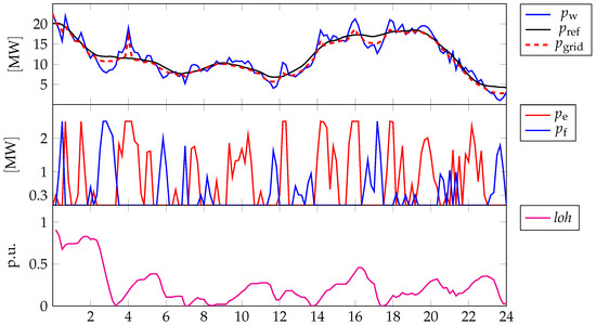
Figure 4. Different profiles related to the reference period from 14:40 of 18 February 2017 to the same hour of 19 February 2017, for highlighting the impact of $c_{\mathrm{N}}^{p_{\mathrm{grid}}}$. First graph: power by wind generation (blue line), power reference that has to be delivered to the grid (black line) and actual power delivered (dashed red line); Second graph: power of the electrolyzer (red line) and power of the fuel cell (blue line); Third graph: LoH.

Figure 5 reports graphs similar to those in Figure 4 but related to the subsequent reference period, i.e., from 14:00 of 19 February 2017 to the same hour of 20 February 2017: the wind generation is very low and this contributes in keeping the LoH low as well. However, at the beginning of the time window, i.e., in between 24 h–26 h, the local peak is used by the controller to produce some hydrogen since the contracted power to be delivered to the grid is smaller. As for the previous reference period, the peak is not totally smoothed because of the limitations of the electrolyzer. Subsequently, the wind generation and the contracted power are practically the same, with very small and scattered around fluctuations of the former in comparison with the latter, such that the controller has no degrees of freedom left in order to boost the LoH. However, what is important to highlight is that the considered peak is barely enough in order to follow the contracted power reference in the immediately following period, even though the negative mismatch between the wind generation and the contracted power therein is small in comparison to the positive similar mismatch in the previous period. This is due to the efficiency of the conversion process determined by the chain electrolyzer-fuel cell, which amounts to roughly 30%.

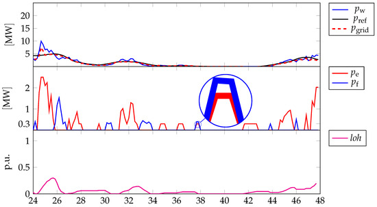
Figure 5. Different profiles related to the reference period 14:40 of 19 February 2017 to the same hour of 20 February 2017, for highlighting the impact of $c_{\mathrm{N}}^{p_{\mathrm{grid}}}$. First graph: power by wind generation (blue line), power reference that has to be delivered to the grid (black line) and actual power delivered (dashed red line); Second graph: power of the electrolyzer (red line) and power of the fuel cell (blue line); Third graph: LoH.

Finally, an interesting consideration regarding the devices’ switchings can be performed: just before 38 h both the electrolyzer and the fuel cell are on and operated about at their minimum power. This may look counterintuitive and counterproductive. However, as remarked in the theoretical development of the devices’ MLD models, mutually exclusive operations are not forced in order to give the controller an extra degree of freedom for the minimization of the switching costs. Anyway, in this case there is no switching cost minimization since the corresponding terms for each device are neglected. Neither this could be justified on the contrary because none of the devices are in on before that time instant. Rather, the mismatch between the wind generation ($p_{\mathrm{w}}\approx 11 \mathrm{k}\mathrm{W}$) and the contracted power ($p_{\mathrm{ref}}\approx 141 \mathrm{k}\mathrm{W}$) cannot be minimized with the sole operations of either the electrolyzer or the fuel cell (depending on the sign of the mismatch) due to their minimum on-power being too high with respect to the hydrogen production/electrification capability required to the purpose. Thus, the controller operates the devices at the same time but with slightly different on-powers ($y_{\mathrm{e}}^{\mathrm{ON}}\approx 300 \mathrm{k}\mathrm{W}$ and $y_{\mathrm{f}}^{\mathrm{ON}}\approx 390 \mathrm{k}\mathrm{W}$) so as to achieve a net effect that would require a device with lower minimum on-power (this outcome can be also leveraged in order to improve the devices’ sizing). Nevertheless, $p_{\mathrm{grid}}\approx 104 \mathrm{k}\mathrm{W}<p_{\mathrm{ref}}$ because of the impact of a very low LoH ($\mathit{loh}\approx 0.04$).

3.2. Scenario 2: Impact of Penalty Fees Cost $c_{\mathrm{N}}^{\mathrm{fee}}$

The impact of $c_{\mathrm{N}}^{\mathrm{fee}}$ is highlighted by simulations carried out with data from the same reference period of Scenario 1 (Section 3.1), such that a comparison is also straightforward. For the other relevant conditions, as before, we refer to Table 3. Moreover, Figure 6 and Figure 7 report the same quantities, with the only addition of the market price profile as second graph, since its relevance in $c_{\mathrm{N}}^{\mathrm{fee}}$. In this case, the control objective is to maximize $c_{\mathrm{N}}^{\mathrm{fee}}$.

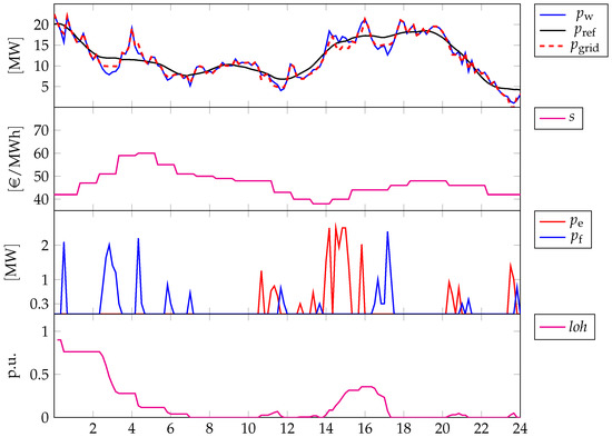
Figure 6. Different profiles related to the reference period from 14:40 of 18 February 2017 to the same hour of 19 February 2017, for highlighting the impact of $c_{\mathrm{N}}^{\mathrm{fee}}$. First graph: power by wind generation (blue line), power reference that has to be delivered to the grid (black line) and actual power delivered (dashed red line); Second graph: spot market prices s (source: “Gestore dei Mercati Energetici s.p.a.—www.mercatoelettrico.org (accessed on 1 July 2022)”); Third graph: power of the electrolyzer (red line) and power of the fuel cell (blue line); Fourth graph: LoH.

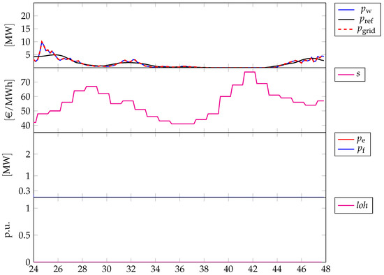
Figure 7. Different profiles related to the reference period 14:40 of 19 February 2017 to the same hour of 20 February 2017, for highlighting the impact of $c_{\mathrm{N}}^{\mathrm{fee}}$. First graph: power by wind generation (blue line), power reference that has to be delivered to the grid (black line) and actual power delivered (dashed red line); Second graph: spot market prices s (source: “Gestore dei Mercati Energetici s.p.a.—www.mercatoelettrico.org (accessed on 1 July 2022)”); Third graph: power of the electrolyzer (red line) and power of the fuel cell (blue line); Fourth graph: LoH.

In the first $24 \mathrm{h}$ the controller operates the electrolyzer and, particularly, the fuel cell such that the negative mismatches between the reference and the power delivered to the grid are within the admissible deviation that does not activate the penalty fees. For instance, in between $2 \mathrm{h}$ and $4 \mathrm{h}$ the fuel cell is operated at about $80\%$ (i.e., approximately $2000 \mathrm{k}\mathrm{W}$), resulting in $p_{\mathrm{grid}}\approx 9934 \mathrm{k}\mathrm{W}$ against $p_{\mathrm{ref}}\approx$ 11,899 kW, and thus in a negative mismatch of approximately $1965 \mathrm{k}\mathrm{W}$. This choice depends on the spot prices that do not promote the activation of the electrolyzer, and, indeed, the wind generation peak at $4 \mathrm{h}$ is not leveraged to produce hydrogen by this means. As a result, the LoH drops dramatically. However, by chance, this has a very negligible impact on the performance of the wind-hydrogen system since the reference profile is tracked without incurring the fees in the following hours. In particular, this is also achieved via the activation of the electrolyzer in between $14 \mathrm{h}$ and $16 \mathrm{h}$ which realizes an increase in the LoH such that the subsequent drop in the wind generation can be mitigated appropriately. Anyway, just a few minutes before $24 \mathrm{h}$, the negative mismatch between the reference profile and the wind generation cannot be prevented because barely any hydrogen is in the tank.

Just by comparing the first $24 \mathrm{h}$ of Scenario 2 and Scenario 1, the different implications of minimizing the sole $c_{\mathrm{N}}^{\mathrm{fee}}$ vs. minimizing the sole $c_{\mathrm{N}}^{p_{\mathrm{grid}}}$ (see Figure 4 and Figure 6, respectively) are apparent. In particular, in Scenario 2 the controller is not committed to tracking a profile, rather it is in charge of not activating the fees and optimizing the revenues by selling energy to the grid. In compliance with this target, e.g., in between $2 \mathrm{h}$ and $4 \mathrm{h}$, the controller produces the minimum effort in order not to activate the fees. This strategy does not promote the activation of the electrolyzer, such that, in terms of the resulting LoH in the tank, this is pretty much more likely to be very low or even zero. The differences between Scenario 2 and 1 are even more obvious by comparing the profiles of the subsequent $24 \mathrm{h}$, i.e., from 14:00 of 19 February 2017 to the same hour of 20 February 2017 (see Figure 5 and Figure 7, respectively). In the case of Scenario 2, i.e., Figure 7, the LoH is zero across all the relevant periods, the electrolyzer and the fuel cell are never activated, such that the entire wind generation is delivered to the grid as is, and no penalties are paid as well. While, in the case of Scenario 1, i.e., Figure 5, the reference profile is better tracked, the electrolyzer and the fuel cell are activated for this purpose and the deriving LoH is less likely to be zero.

3.3. Scenario 3: Impact of Hydrogen Value Cost $c_{\mathrm{N}}^{\mathit{loh}}$

In Scenario 3 the impact of the optimization of the sole $c_{\mathrm{N}}^{\mathit{loh}}$ is presented (see Table 3 for reference). The chosen relevant period for the numerical simulations is the same as the previous scenarios. Moreover, the relevant quantities are arranged differently, with the reference profile being not shown: the first graph reports the wind generation (blue line) and the power delivered to the grid (dashed red line); the second graph reports the electrolyzer (red line) and the fuel cell (blue line) powers; the third graph reports the LoH. In this case, the control objective is to maximize $c_{\mathrm{N}}^{\mathit{loh}}$. In this sense, in order to set an adverse initial condition, LoH is set to 0.1, while in the previous scenarios was 0.9.

As Figure 8 shows, the controller operates the devices consistently with the objective. The electrolyzer is switched on at maximum power such that the LoH increases to the maximum. Subsequently, the electrolyzer is switched to stand-by, and the power delivered to the grid matches exactly that of wind generation.

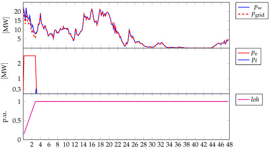
Figure 8. Different profiles related to the reference period from 14:40 of 18 February 2017 to the same hour of 20 February 2017, for highlighting the impact of $c_{\mathrm{N}}^{\mathit{loh}}$. First graph: power by wind generation (blue line) and power delivered to the grid (dashed red line); Second graph: power of the electrolyzer (red line) and power of the fuel cell (blue line); Fourth graph: Level of Hydrogen (LoH).

3.4. Scenario 4: Full-Feature Operations with N = 18

In this scenario, all the cost terms developed in the article are included in the controller. The cost weights are chosen as per Table 3, following a number of simulations in order to find a good balance among all the (conflicting) objectives.

The relevant period for the assessment of the performances is the same as of the previous scenarios, as Figure 9 and Figure 10 show. Across the whole time interval, fees are never activated, as the controller manages to mitigate the lack of renewable generation. For instance, this is highlighted in Figure 9, in between 2 h–4 h: the controller operates the fuel cell at full power with a subsequent steep drop of the LoH. However, as the renewable generation increases rapidly till a local peak, the fuel cell is switched to stand-by and the electrolyzer is operated at full power. In this case, the competing terms in the optimizer are $c_{\mathrm{N}}^{\mathrm{fee}}$ and $c_{\mathrm{N}}^{\mathit{loh}}$, with a lesser dominance of the former with respect to the latter. Thus, in spite of increasing spot prices, the positive peak in the generation is mitigated and used for hydrogen production. This helps the controller to oppose the future drops in the renewable generation via an appropriate re-electrification of the hydrogen. Anyway, as a tendency, the LoH is mostly likely to stay below 0.5 (with the initial condition set to 0.9), which suggests that the priority to the hydrogen production is appropriate (also because no fees are paid, as already noted) for the first timespan. Instead, in the subsequent 24 h, as Figure 10 shows, wind variability is minor and LoH increases notwithstanding some peaks in the spot prices which instead could be leveraged by the controller. However, selecting different values of the weights would not produce any improvement because the lesser the tendency to keep the hydrogen stored in the tank the higher the possibility that the controller uses this “degree of freedom” during the first 24 h, with the implication that in the second 24 h the LoH would be so low to prevent to re-electrify it anyway. In practice, setting dynamically the weights could be a possible solution.

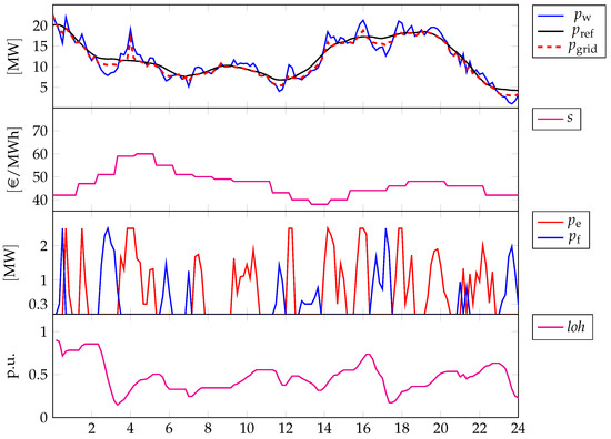
Figure 9. Different profiles related to the reference period from 14:40 of 18 February 2017 to the same hour of 19 February 2017, with full-feature operations. First graph: power by wind generation (blue line), power reference that has to be delivered to the grid (black line) and actual power delivered (dashed red line); Second graph: spot market prices s (source: “Gestore dei Mercati Energetici s.p.a.—www.mercatoelettrico.org (accessed on 1 July 2022)”); Third graph: power of the electrolyzer (red line) and power of the fuel cell (blue line); Fourth graph: LoH.

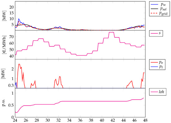
Figure 10. Different profiles related to the reference period from 14:40 of 19 February 2017 to the same hour of 20 February 2017, with full-feature operations. First graph: power by wind generation (blue line), power reference that has to be delivered to the grid (black line) and actual power delivered (dashed red line); Second graph: spot market prices s (source: “Gestore dei Mercati Energetici s.p.a.—www.mercatoelettrico.org (accessed on 1 July 2022)”); Third graph: power of the electrolyzer (red line) and power of the fuel cell (blue line); Fourth graph: LoH.

3.5. Full-Feature Operations in Spring/Summer with N = 18 vs. N = 60

In this section, the effects of different prediction horizons in the same target period, i.e., Scenario 5 vs. Scenario 6, are highlighted, and the corresponding strategies are compared. In order to mitigate the bias of the single cost terms resulting naturally from the increase in the prediction horizon, their weights for $\mathrm{N}=60$ are standardized against the horizon such that their averages across the whole simulation time amount to the same as the averages of the terms in case of $\mathrm{N}=18$.

Figure 11 and Figure 12 show the different strategies provided by the controller within the first and the second $24 \mathrm{h}$, respectively, of 29 May 2017, with initial time set to 09:00 and initial condition for LoH set to 0.1. There, similar quantities as those in the previous discussions are presented, with the difference that dashed lines are used to indicate the evolutions of relevant quantities when pertaining to the strategy for $\mathrm{N}=60$.

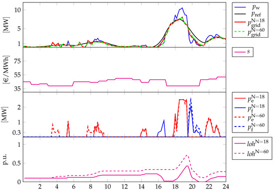
Figure 11. Different profiles related to the reference period from 09:00 of 29 May 2017 to the same hour of 30 May 2017, with full-feature operations: $\mathrm{N}=18$ vs. $\mathrm{N}=60$. First graph: power by wind generation (blue solid line), power reference that has to be delivered to the grid (black solid line), actual power delivered when $\mathrm{N}=18$ (red solid line) and actual power delivered when $\mathrm{N}=60$ (green dashed line); Second graph: spot market prices s (source: “Gestore dei Mercati Energetici s.p.a.—www.mercatoelettrico.org (accessed on 1 July 2022)”); Third graph: power of the electrolyzer when $\mathrm{N}=18$ (red solid line), power of the fuel cell when $\mathrm{N}=18$ (blue solid line), power of the electrolyzer when $\mathrm{N}=60$ (red dashed line) and power of the fuel cell when $\mathrm{N}=60$ (blue dashed line); Fourth graph: LoH when $\mathrm{N}=18$ (magenta solid line) and LoH when $\mathrm{N}=60$ (magenta dashed line).

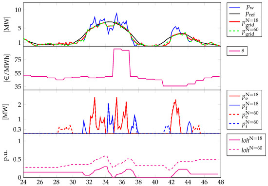
Figure 12. Different profiles related to the reference period from 09:00 of 30 May 2017 to the same hour of 31 May 2017, with full-feature operations: $\mathrm{N}=18$ vs. $\mathrm{N}=60$. First graph: power by wind generation (blue solid line), power reference that has to be delivered to the grid (black solid line), actual power delivered when $\mathrm{N}=18$ (red solid line) and actual power delivered when $\mathrm{N}=60$ (green dashed line); Second graph: spot market prices s (source: “Gestore dei Mercati Energetici s.p.a.—www.mercatoelettrico.org (accessed on 1 July 2022)”); Third graph: power of the electrolyzer when $\mathrm{N}=18$ (red solid line), power of the fuel cell when $\mathrm{N}=18$ (blue solid line), power of the electrolyzer when $\mathrm{N}=60$ (red dashed line) and power of the fuel cell when $\mathrm{N}=60$ (blue dashed line); Fourth graph: LoH when $\mathrm{N}=18$ (magenta solid line) and LoH when $\mathrm{N}=60$ (magenta dashed line).

As it is possible to notice, even though at first look the strategies might seem rather similar, they imply remarkable differences in the time evolution of the LoHs. In case of $\mathrm{N}=18$, the achieved LoH keeps generally low across the two days. While, in the case of $\mathrm{N}=60$, the controller manages to achieve an increasing evolution till $\mathit{loh}=0.5$ at the end of the second day. The differences in terms of $p_{\mathrm{grid}}$ are subtle, however, they are remarked by the different activation of the electrolyzer and the fuel cell. In case of $\mathrm{N}=60$, the controller tends to produce hydrogen more than in the case of $\mathrm{N}=18$, which is highlighted, for instance, by the activation of the electrolyzer about $4 \mathrm{h}$ and in between $8 \mathrm{h}$ and $10 \mathrm{h}$, roughly, or by the non activation of the fuel cell just about $16 \mathrm{h}$ and the subsequent minutes. This more conservative strategy is achieved without incurring any fee, as ${\delta }^{\mathrm{fee}}$ keeps null across the entire simulation window (clearly the same happens when $\mathrm{N}=18$ is considered). The differences in the strategy are highlighted also in the plots related to the second day, especially looking at those reporting the devices’ powers. In both cases, however, the peak in the spot prices is not leveraged for minimizing the costs accounted for by the term $c_{\mathrm{N}}^{\mathrm{fee}}$. Actually, this can be achieved by a different choice of the corresponding weight, i.e., increasing it such that, e.g., $c_{\mathrm{N}}^{\mathrm{fee}}$ becomes higher than $c_{\mathrm{N}}^{p_{\mathrm{grid}}}$. However, we remark that the choice is nontrivial in general, as also highlighted in Figure 13. In this figure, the strategies for two different choices of $c_{\mathrm{N}}^{\mathrm{fee}}$ are reported, where solid lines denote the strategies achieved when the parameters, in general, and $c_{\mathrm{N}}^{\mathrm{fee}}$ in particular, are as per Table 3, while dashed lines denote the strategies achieved when $c_{\mathrm{N}}^{\mathrm{fee}}$ is increased to 3. Further, the whole two-days relevant period is addressed such that it is easy to check that fixed weights can be ineffective in some circumstances. The two strategies derive also from two different choices for the initial conditions of LoH, where, in the case of $c_{\mathrm{N}}^{\mathrm{fee}}=0.013$ (benchmark), the initial condition is set to $0.1$ while, in the case of $c_{\mathrm{N}}^{\mathrm{fee}}=3$, the initial condition is set to $0.9$, such that being the second strategy less conservative, this aspect can be better highlighted. The differences can be noted just within the first $24 \mathrm{h}$, where, in case of the benchmark value of $c_{\mathrm{N}}^{\mathrm{fee}}$, the evolution of the LoH is increasing due to the various activations of the electrolyzer. This results in small yet impactful differences in $p_{\mathrm{grid}}$ that lead to a general LoH decrease when $c_{\mathrm{N}}^{\mathrm{fee}}$ is higher. Clearly, the higher priority given to the earnings from selling energy to the grid increases the tendency of not keeping too much hydrogen in the tank and/or not to produce hydrogen in case of (local) renewable peaks.

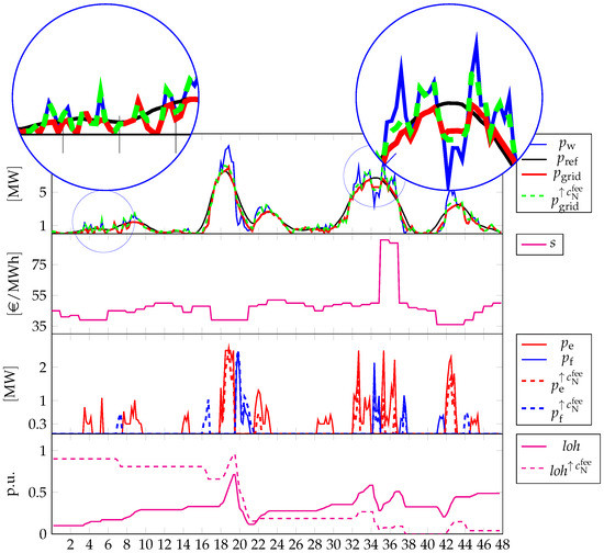
Figure 13. Different profiles related to the reference period from 09:00 of 29 May 2017 to the same hour of 30 May 2017, with full-feature operations: $c_{\mathrm{N}}^{\mathrm{fee}}=0.2$ vs. $c_{\mathrm{N}}^{\mathrm{fee}}=3$. First graph: power by wind generation (blue solid line), power reference that has to be delivered to the grid (black solid line), actual power delivered when $c_{\mathrm{N}}^{\mathrm{fee}}=0.2$ (red solid line) and actual power delivered when $c_{\mathrm{N}}^{\mathrm{fee}}=3$ (green dashed line); Second graph: spot market prices s (source: “Gestore dei Mercati Energetici s.p.a.—www.mercatoelettrico.org (accessed on 1 July 2022)”); Third graph: power of the electrolyzer when $c_{\mathrm{N}}^{\mathrm{fee}}=0.2$ (red solid line), power of the fuel cell when $c_{\mathrm{N}}^{\mathrm{fee}}=0.2$ (blue solid line), power of the electrolyzer when $c_{\mathrm{N}}^{\mathrm{fee}}=3$ (red dashed line) and power of the fuel cell when $c_{\mathrm{N}}^{\mathrm{fee}}=3$ (blue dashed line); Fourth graph: LoH when $c_{\mathrm{N}}^{\mathrm{fee}}=0.2$ (magenta solid line) and LoH when $c_{\mathrm{N}}^{\mathrm{fee}}=3$ (magenta dashed line).

This tendency is confirmed in the subsequent 24 h, where in case of the increased $c_{\mathrm{N}}^{\mathrm{fee}}$ the LoH is decreasing. In particular, in between 35 h–40 h, even though the LoH is very low, the controller leverages the local peak in the spot market to inject power into the grid at current prices, notwithstanding this implies zero LoH in the immediate forthcoming time period, while this choice is not adopted in the case of the benchmark $c_{\mathrm{N}}^{\mathrm{fee}}$. Possibly, a bigger tank could mitigate this decrease, in combination, as also pinpointed earlier, with the adoption of a dynamic weighting, which could also be a possible future research direction.

4. Discussion

This paper targets smooth power injection for wind farms paired to a HESS as established by the IEA in the final report of Task 24 operating under the HIA and published in 2013. This operating mode is considered one among the possible three that can promote the integration of wind generation into the grid and is not exactly covered by the actual literature. The paper develops an MPC strategy that relies on MLD modeling for the electrolyzer and the fuel cell, such that they can be operated by providing suitable logic commands and a continuous amount of powers they have to convert into hydrogen/re-electrify. The control strategy is demonstrated considering generation profiles of a real wind farm located in the center-south of Italy and corresponding real spot market prices. The addressed system and scenario are similar to those in [8], which shares some of the authors of this paper, however with a number of different assumptions, closer to a realistic application, that leads to quite different modeling and results. In addition to power smoothing, the control algorithms also include additional cost terms in order to account for the inherent value of the produced hydrogen and in order to account for the fees that the wind farm owner/operator might incur in case of infringement of the agreement with the TSO on the contracted power to be delivered to the grid.

The proposed controller shows enough flexibility to balance against different and competing objectives in real scenarios, providing that an appropriate choice of weights is adopted. In this regard, the simulations show that a dynamic choice of the weights corresponding to the costs and revenues that are optimized could be more appropriate since the controller performances can be strongly affected by the combination of the system conditions (e.g., the LoH in the tank) with the various exogenous’ (e.g., the renewable generation and market prices). This, in general, can be a possible investigation research. Another possible research direction is identified by the use of the developed models and algorithms in order to carry out a scenario analysis with the aim of achieving different wind-hydrogen system sizes against multiple renewable generations and spot market profiles. The outcomes can be fruitfully used for a sizing that also accounts for the minimization of the devices’ operating costs, among the many.

References

- Hoskin, A.; Pedersen, A.S.; Varkaraki, E.; Pino, F.J.; Aso, I.; Simón, J.; Lehmann, J.; Linnemann, J.; Stolzenburg, K.; Castrillo, L.; et al. IEA-HIA Task 24—Wind Energy & Hydrogen Integration—Final Report; Technical Report; International Energy Agency-Hydrogen Implementing Agreement. 2013. Available online: https://www.ieahydrogen.org/wpfd_file/task-24-final-report/ (accessed on 29 August 2022).
- Zhao, X.; Yan, Z.; Xue, Y.; Zhang, X.P. Wind Power Smoothing by Controlling the Inertial Energy of Turbines with Optimized Energy Yield. IEEE Access 2017, 5, 23374–23382. [Google Scholar] [CrossRef]
- Lyu, X.; Zhao, J.; Jia, Y.; Xu, Z.; Po Wong, K. Coordinated Control Strategies of PMSG-Based Wind Turbine for Smoothing Power Fluctuations. IEEE Trans. Power Syst. 2019, 34, 391–401. [Google Scholar] [CrossRef]
- Lyu, X.; Jia, Y.; Xu, Z.; Ostergaard, J. Mileage-Responsive Wind Power Smoothing. IEEE Trans. Ind. Electron. 2020, 67, 5209–5212. [Google Scholar] [CrossRef]
- Mahmoudi, N.; Saha, T.K.; Eghbal, M. Wind Power Offering Strategy in Day-Ahead Markets: Employing Demand Response in a Two-Stage Plan. IEEE Trans. Power Syst. 2015, 30, 1888–1896. [Google Scholar] [CrossRef]
- Li, C.; Yao, Y.; Zhao, C.; Wang, X. Multi-Objective Day-Ahead Scheduling of Power Market Integrated With Wind Power Producers Considering Heat and Electricity Trading and Demand Response Programs. IEEE Access 2019, 7, 181213–181228. [Google Scholar] [CrossRef]
- Yang, Y.; Qin, C.; Zeng, Y.; Wang, C. Optimal Coordinated Bidding Strategy of Wind and Solar System with Energy Storage in Day-ahead Market. J. Mod. Power Syst. Clean Energy 2022, 10, 192–203. [Google Scholar] [CrossRef]
- Abdelghany, M.B.; Faisal Shehzad, M.; Liuzza, D.; Mariani, V.; Glielmo, L. Modeling and Optimal Control of a Hydrogen Storage System for Wind Farm Output Power Smoothing. In Proceedings of the 2020 59th IEEE Conference on Decision and Control (CDC), Jeju, Korea, 14–18 December 2020; pp. 49–54. [Google Scholar] [CrossRef]
- Koiwa, K.; Ishii, T.; Liu, K.Z.; Zanma, T.; Tamura, J. On the Reduction of the Rated Power of Energy Storage System in Wind Farms. IEEE Trans. Power Syst. 2020, 35, 2586–2596. [Google Scholar] [CrossRef]
- Yang, M.; Zhang, L.; Cui, Y.; Zhou, Y.; Chen, Y.; Yan, G. Investigating the Wind Power Smoothing Effect Using Set Pair Analysis. IEEE Trans. Sustain. Energy 2020, 11, 1161–1172. [Google Scholar] [CrossRef]
- Barra, P.; de Carvalho, W.; Menezes, T.; Fernandes, R.; Coury, D. A review on wind power smoothing using high-power energy storage systems. Renew. Sustain. Energy Rev. 2021, 137, 110455. [Google Scholar] [CrossRef]
- Lamsal, D.; Sreeram, V.; Mishra, Y.; Kumar, D. Output power smoothing control approaches for wind and photovoltaic generation systems: A review. Renew. Sustain. Energy Rev. 2019, 113, 109245. [Google Scholar] [CrossRef]
- Zhai, Y.; Zhang, J.; Tan, Z.; Liu, X.; Shen, B.; Coombs, T.; Liu, P.; Huang, S. Research On the Application of Superconducting Magnetic Energy Storage in the Wind Power Generation System For Smoothing Wind Power Fluctuations. IEEE Trans. Appl. Supercond. 2021, 31, 1–5. [Google Scholar] [CrossRef]
- Yang, R.H.; Jin, J.X. Unified Power Quality Conditioner with Advanced Dual Control for Performance Improvement of DFIG-Based Wind Farm. IEEE Trans. Sustain. Energy 2021, 12, 116–126. [Google Scholar] [CrossRef]
- Wang, B.; Cai, G.; Yang, D. Dispatching of a Wind Farm Incorporated With Dual-Battery Energy Storage System Using Model Predictive Control. IEEE Access 2020, 8, 144442–144452. [Google Scholar] [CrossRef]
- Sattar, A.; Al-Durra, A.; Caruana, C.; Debouza, M.; Muyeen, S.M. Testing the Performance of Battery Energy Storage in a Wind Energy Conversion System. IEEE Trans. Ind. Appl. 2020, 56, 3196–3206. [Google Scholar] [CrossRef]
- Wan, C.; Qian, W.; Zhao, C.; Song, Y.; Yang, G. Probabilistic Forecasting Based Sizing and Control of Hybrid Energy Storage for Wind Power Smoothing. IEEE Trans. Sustain. Energy 2021, 12, 1841–1852. [Google Scholar] [CrossRef]
- Spichartz, B.; Günther, K.; Sourkounis, C. New Stability Concept for Primary Controlled Variable Speed Wind Turbines Considering Wind Fluctuations and Power Smoothing. IEEE Trans. Ind. Appl. 2022, 58, 2378–2388. [Google Scholar] [CrossRef]
- De Battista, H.; Mantz, R.J.; Garelli, F. Power conditioning for a wind-hydrogen energy system. J. Power Sources 2006, 155, 478–486. [Google Scholar] [CrossRef]
- Little, M.; Thomson, M.; Infield, D. Electrical integration of renewable energy into stand-alone power supplies incorporating hydrogen storage. Int. J. Hydrogen Energy 2007, 32, 1582–1588. [Google Scholar] [CrossRef]
- Takahashi, R.; Kinoshita, H.; Murata, T.; Tamura, J.; Sugimasa, M.; Komura, A.; Futami, M.; Ichinose, M.; Ide, K. Output Power Smoothing and Hydrogen Production by Using Variable Speed Wind Generators. IEEE Trans. Ind. Electron. 2010, 57, 485–493. [Google Scholar] [CrossRef]
- Muyeen, S.; Takahashi, R.; Tamura, J. Electrolyzer switching strategy for hydrogen generation from variable speed wind generator. Electr. Power Syst. Res. 2011, 81, 1171–1179. [Google Scholar] [CrossRef]
- Wen, T.; Zhang, Z.; Lin, X.; Li, Z.; Chen, C.; Wang, Z. Research on Modeling and the Operation Strategy of a Hydrogen-Battery Hybrid Energy Storage System for Flexible Wind Farm Grid-Connection. IEEE Access 2020, 8, 79347–79356. [Google Scholar] [CrossRef]
- Huang, C.; Zong, Y.; You, S.; Træholt, C.; Zheng, Z.; Xie, Q. Cooperative Control of Wind-Hydrogen-SMES Hybrid Systems for Fault-Ride-Through Improvement and Power Smoothing. IEEE Trans. Appl. Supercond. 2021, 31, 1–7. [Google Scholar] [CrossRef]
- Koiwa, K.; Cui, L.; Zanma, T.; Liu, K.Z.; Tamura, J. A Coordinated Control Method for Integrated System of Wind Farm and Hydrogen Production: Kinetic Energy and Virtual Discharge Controls. IEEE Access 2022, 10, 28283–28294. [Google Scholar] [CrossRef]
- Bemporad, A.; Morari, M. Control of systems integrating logic, dynamics, and constraints. Automatica 1999, 35, 407–427. [Google Scholar] [CrossRef]
- Williams, P.H. Model Building in Mathematical Programmin, 5th ed.; John Wiley & Sons Ltd.: Hoboken, NJ, USA, 2013. [Google Scholar]
- Bynum, M.L.; Hackebeil, G.A.; Hart, W.E.; Laird, C.D.; Nicholson, B.L.; Siirola, J.D.; Watson, J.P.; Woodruff, D.L. Pyomo–Optimization Modeling in Python, 3rd ed.; Springer: Berlin/Heidelberg, Germany, 2021; Volume 67. [Google Scholar]
- Hart, W.E.; Watson, J.P.; Woodruff, D.L. Pyomo: Modeling and solving mathematical programs in Python. Math. Program. Comput. 2011, 3, 219–260. [Google Scholar]
- Pyomo.org. 2022. Available online: http://www.pyomo.org/ (accessed on 1 July 2022).
- FICO. 2022. Available online: https://www.fico.com/en/products/fico-xpress-optimization (accessed on 1 July 2022).
- Friendly Power S.r.l. 2022. Available online: http://www.friendlypower.it/ (accessed on 1 July 2022).
- GME—Gestore Mercati Energetici. 2022. Available online: http://www.mercatoelettrico.org/ (accessed on 1 July 2022).
- Atif, A.; Khalid, M. Saviztky-Golay Filtering for Solar Power Smoothing and Ramp Rate Reduction Based on Controlled Battery Energy Storage. IEEE Access 2020, 8, 33806–33817. [Google Scholar] [CrossRef]
Publisher’s Note: MDPI stays neutral with regard to jurisdictional claims in published maps and institutional affiliations. |
© 2022 by the authors. Licensee MDPI, Basel, Switzerland. This article is an open access article distributed under the terms and conditions of the Creative Commons Attribution (CC BY) license (https://creativecommons.org/licenses/by/4.0/).