Three-Phase State Estimation of a Low-Voltage Distribution Network with Kalman Filter

Abstract

The state estimation of distribution networks has long been considered a challenging task for the reduced availability of real-time measures with respect to the transmission network case. This issue is expected to be improved by the deployment of modern smart meters that can be polled at relatively short time intervals. On the other hand, the management of the information coming from many heterogeneous meters still poses major issues. If low-voltage distribution systems are of interest, a three-phase formulation should be employed for the state estimation due to the typical load imbalance. Moreover, smart meter data may not be perfectly synchronized. This paper presents the implementation of a three-phase state estimation algorithm of a real portion of a low-voltage distribution network with distributed generation equipped with smart meters. The paper compares the typical state estimation algorithm that implements the weighted least squares method with an algorithm based on an iterated Kalman filter. The influence of nonsynchronicity of measurements and of delays in communication and processing is analyzed for both approaches.

1. Introduction

The main task of a distribution management system (DMS) is to monitor and control the distribution networks to guarantee system reliability, efficiency, security, and resiliency. In order to accomplish such objective, different control functionalities are implemented in the DMS, such as state estimation (SE) [1].

While the SE of transmission networks is a well-known practice, the SE of distribution systems is more recent, and introduces new perspectives and issues with respect to transmission networks: the monitoring of many buses and the system observability requirement are among the main problems. With the advent of automated meter reading and the corresponding advanced metering infrastructure needed to accomplish it, a valuable quantity of measurements is now available, mainly coming from smart meters (SMs), but other sources of measurement might become available in the future, such as digital relays, smart inverters, smart transformers, automated switches, and voltage regulators [2]. Moreover, distribution systems are usually unbalanced, and single-phase or two-phase lines might be present. Thus, the SE problem must be dealt with in a three-phase formulation.

The most common technique used for the static SE of power systems adopts the weighted least squares (WLS) method [3], while the use of different implementations of the Kalman filter (KF) [4,5] are proposed to solve dynamic or quasi-dynamic SE. The SE obtained by using the KF is a trade-off between the state predicted by the dynamic model of the system and the state estimated by using the most recent information available. The use of the KF with linearized functions of the dynamic model and of the relationship between measurements and state variables is usually referred to as an extended Kalman filter (EKF), while its iterative use is known as an iterated Kalman filter (IKF). The IKF can be advantageously used in a power system SE when a dynamic model is available, e.g., by using load forecast data, as in [6]. The IKF presents some advantages with respect to the WLS method because it allows the inclusion of past measurements in the SE problem, even in the absence of a well-identified process model, as shown in [7,8]. Different KF implementations were successfully applied to the SE problem, other than the EKF, e.g., the particle filter [9], the unscented KF [10], and the ensemble KF [11]. In the relevant literature, several methods have been proposed for the SE of power systems [12,13], among which are M-estimators [14], Bayesian inference approaches [15], deep-learning techniques [16,17], and clustering algorithms [18].

The performance of the KFs is largely affected by the process uncertainties, and specific approaches are proposed to manage the model noise [19], the changing operation conditions of the power system [20], and the data losses [21]. The measurement delays or losses can have a major influence on the performance of an SE algorithm and are included in the main aspects addressed in this paper.

Most KF-SE algorithms for distribution systems (e.g., [7,8,11,19,20,21,22]) assume the presence of phasor measurement units (PMUs) [23]. Unlike PMUs, SMs acquire the measurements in long time intervals, typically 15 min, and report them to the data center with considerable latencies [24]. Few papers address the problem of SE using SMs (e.g., [24,25]) but none of them implemented a KF-based approach.

This paper extends the algorithms based on WLS and KF-SE presented in [7] to the three-phase formulation. The two algorithms are tested by considering a real three-phase, four-wire low-voltage (LV) system. The LV system is fed by a secondary substation of the distribution system operator (DSO) AMAIE, located in the suburban area of the city of San Remo, Italy. The development of the SE functionality of the DMS was carried out in the framework of project PODCAST (platform for the optimization of the distribution using data from smart meters and distributed storage systems), which was recently terminated [26]. The paper compares the results obtained by using the WLS-SE algorithm and the KF-SE algorithm, and analyzes the influence of the nonsynchronicity between the measurements as well as the latency due to communication network limits and data processing. The main contributions of this paper are threefold: (i) the application of a three-phase SE in a real LV system with distributed generation; (ii) the implementation of a KF for the SE of a system monitored with low-rate measurement devices, such as the SMs employed in the analyzed network; and (iii) the analysis of the influence of both the nonsynchronicity and the time latencies due to process and communication delays on the performance of the SE.

The paper is organized as follows. Section 2 presents the formulation of the SE problem by introducing the WLS-SE and the KF-SE algorithms in a single-phase formulation and the extension to the three-phase one. Section 3 presents the considered real LV network. Section 4 presents the analysis of the results obtained by using both algorithms. The conclusions are drawn in Section 5, and some perspectives for future developments are given.

2. Formulation of the State Estimation Problem

This section reviews the SE formulation in both single-phase and three-phase implementation.

2.1. Single-Phase State Estimation

Let N be the number of buses in the network. The system state vector x is composed of the voltage phasor angles and magnitudes of all buses expressed in polar coordinates. The phase angle of one bus is taken as reference, so x is an n-row vector with n = 2N − 1, although it could be convenient to estimate all the phase angles in presence of PMUs [27]. Assuming bus 1 as reference, it follows that [3]:

$$\mathbf{x}={\left[{\delta }_2,\dots ,{\delta }_N,V_1,\dots ,V_N\right]}^{\mathrm{T}},$$

(1)

where δ_i and V_i represent the voltage phasor angle and magnitude of the of i-th bus, respectively.

Consider the vector z comprising a set of m measurements; the j-th measurement is given by:

$$z_j=h_j(x_1,\dots ,x_i,\dots ,x_n)+e_j,$$

(2)

where h_j is a relation, generally nonlinear [4], between the measurement z_j and the state vector x; and e_j is the corresponding measurement error, usually assumed to be random and independent, and represented by a function with normal probability distribution and null mean value. Non-normal systematic errors, such as those produced by the sensors [28], are here neglected. From (2), it follows that the residuals, i.e., the difference between the measured and the estimated values is:

$${e_j|}_{\widehat{\mathbf{x}}}=z_j-h_j(\widehat{\mathbf{x}}).$$

(3)

Hatted variables represent the estimated quantities. [3]. The WLS-SE consists of minimizing the weighted sum of the squares of the errors, i.e., minimizing the objective function:

$$f={\displaystyle \sum _{j=1}^m{w}_j{e}_j^2},$$

(4)

where w_j is the assigned weight of the error e_j.

The function is minimum when:

$${\displaystyle \sum _{j=1}^m\left(w_j{e_j|}_{\widehat{\mathbf{x}}}{\frac{\partial e_j}{\partial x_i}|}_{\widehat{\mathbf{x}}}\right)}=0\hspace{1em}(i=1\dots n),$$

(5)

The solution of (5) is found by an iterative algorithm. Considering the v-th iteration, (3) is written as:

$$e_j^{\left(v\right)}=z_j-h_j({\widehat{\mathbf{x}}}^{\left(v\right)}).$$

(6)

Linearizing h_j around v − 1 by implementing the first order Taylor series, it yields:

$$h_j({\widehat{\mathbf{x}}}^{\left(v\right)})=h_j({\widehat{\mathbf{x}}}^{\left(v-1\right)})+{\displaystyle \sum _{k=1}^n\left({\frac{\partial h_j}{\partial x_k}|}_{{\widehat{x}}_k^{\left(v-1\right)}}\Delta {\widehat{x}}_k^{\left(v\right)}\right)},$$

(7)

with $\Delta {\widehat{x}}_i^{\left(v\right)}={\widehat{x}}_i^{\left(v\right)}-{\widehat{x}}_i^{\left(v-1\right)}$. Replacing (7) in (6), it gives:

$$e_j^{\left(v\right)}=z_j-h_j({\widehat{x}}^{\left(v-1\right)})-{\displaystyle \sum _{k=1}^n\left({\frac{\partial h_j}{\partial x_k}|}_{{\widehat{x}}_k^{\left(v-1\right)}}\Delta {\widehat{x}}_k^{\left(v\right)}\right)},$$

(8)

from which:

$$e_j^{\left(v\right)}=e_j^{\left(v-1\right)}-{\displaystyle \sum _{k=1}^n\left({\frac{\partial h_j}{\partial x_k}|}_{{\widehat{x}}_k^{\left(v-1\right)}}\Delta {\widehat{x}}_k^{\left(v\right)}\right)},$$

(9)

then:

$${\frac{\partial e_j}{\partial x_k}|}_{\widehat{\mathbf{x}}}=-{\frac{\partial h_j}{\partial x_k}|}_{\widehat{\mathbf{x}}}.$$

(10)

Replacing (9) and (10) in (5) yields:

$${\displaystyle \sum _{j=1}^m\left\{{\frac{\partial h_j}{\partial x_i}|}_{{\widehat{\mathbf{x}}}^{(v-1)}}{w}_j\left[e_j^{(v-1)}-{\displaystyle \sum _{k=1}^n\left({\frac{\partial h_j}{\partial x_k}|}_{{\widehat{x}}_k^{\left(v-1\right)}}\Delta {\widehat{x}}_k^{\left(v\right)}\right)}\right]\right\}=0}\hspace{1em}(i=1\dots n)$$

(11)

By introducing measurement Jacobian matrix H, (11) in matrix form becomes:

$${\widehat{\mathbf{H}}}^{\left(v-1\right)}{}^{\mathrm{T}}\mathbf{W}{\mathbf{e}}^{\left(v-1\right)}={\widehat{\mathbf{H}}}^{\left(v-1\right)}{}^{\mathrm{T}}\mathbf{W}{\widehat{\mathbf{H}}}^{\left(v-1\right)}\Delta {\widehat{\mathbf{x}}}^{\left(v\right)},$$

(12)

which constitutes an n-equation system. $\widehat{\mathbf{H}}$ is an m-by-n matrix, e an m-column vector, and $\Delta \widehat{\mathbf{x}}$ an n-column vector. W is a diagonal m-by-m matrix given by:

$$\mathbf{W}=\mathrm{diag}(w_1,\dots ,w_m).$$

(13)

Weights are usually selected to make more accurate measurements having a greater influence on the SE. This can be achieved by constructing the measurement noise covariance matrix R considering the measurement variances ${\sigma }_j^2$:

$$\mathbf{R}=\mathrm{diag}({\sigma }_1^2, \dots ,{\sigma }_m^2),$$

(14)

then:

$$\mathbf{W}={\mathbf{R}}^{-1}.$$

(15)

From (12) and (15), $\Delta \widehat{\mathbf{x}}$ is derived:

$$\Delta {\widehat{\mathbf{x}}}^{\left(v\right)}={\left({\mathbf{G}}^{\left(v-1\right)}\right)}^{-1}{\widehat{\mathbf{H}}}^{\left(v-1\right)}{}^{\mathrm{T}}{\mathbf{R}}^{-1}{\mathbf{e}}^{\left(v-1\right)},$$

(16)

where the matrix G:

$$\mathbf{G}={\widehat{\mathbf{H}}}^{\mathrm{T}}{\mathbf{R}}^{-1}\widehat{\mathbf{H}}$$

(17)

is the gain matrix, symmetric and sparse, although less sparse than H [3]. It results that:

$${\widehat{\mathbf{x}}}^{\left(v\right)}={\widehat{\mathbf{x}}}^{\left(v-1\right)}+\Delta {\widehat{\mathbf{x}}}^{\left(v\right)},$$

(18)

and the iterative process is repeated until:

$$f_v<{\mathit{tol}}_1\hspace{1em}\mathrm{or}\hspace{1em}{f}_v-f_{v-1}<{\mathit{tol}}_2;$$

(19)

i.e., until either the objective function or its difference with respect to the previous iteration is minor than the given tolerances.

2.2. The Kalman Filter Implementation

The KF represents a recursive solution of the least squares method [29] obtained by implementing a discrete model of the process in order to estimate the dynamic variation of the state variables. The state vector can be a generic nonlinear dynamic system, for which at the κ-instant it depends on the previous state through the function φ as follows:

$${\mathbf{x}}_{\kappa }=\phi \left({\mathbf{x}}_{\kappa -1},{\mathsf{\nu }}_{\kappa -1}\right),$$

(20)

where ν is a white-noise sequence following a normal probability distribution with null mean value, uncorrelated from the measurement noise. The discrete Kalman filter (DKF) implementation assumes linear measurement and process models, for which the residuals in (3) and the process model in (20) can be respectively expressed as:

$${\mathbf{e}}_{\kappa }={\mathbf{z}}_{\kappa }-\mathbf{H}{\widehat{\mathbf{x}}}_{\kappa },$$

(21)

$${\mathbf{x}}_{\kappa }={\mathsf{\Phi }}_{\kappa ,\kappa -1}{\mathbf{x}}_{\kappa -1}+{\mathsf{\nu }}_{\kappa -1},$$

(22)

where Ф_κ,κ-1 is the state-transition matrix, which relates the states at the κ- and (κ − 1)-instants. H is time-independent and is defined by the network topology.

In absence of new data, (22) provides a predicted estimated state, i.e., an a priori estimate, given by:

$${\widehat{\mathbf{x}}}_{\kappa |\kappa -1}={\mathsf{\Phi }}_{\kappa ,\kappa -1}{\widehat{\mathbf{x}}}_{\kappa -1|\kappa -1}.$$

(23)

The final state estimate is the result of the linear combination of the a priori estimate and the residuals, and it has the following form:

$${\widehat{\mathbf{x}}}_{\kappa |\kappa }={\mathsf{\Phi }}_{\kappa ,\kappa -1}{\widehat{\mathbf{x}}}_{\kappa -1|\kappa -1}+{\mathbf{K}}_{\kappa }\left({\mathbf{z}}_{\kappa }-{\mathbf{H}}_{\kappa }{\widehat{\mathbf{x}}}_{\kappa |\kappa -1}\right),$$

(24)

resulting in the a posteriori estimate. The term ${\mathbf{z}}_{\kappa }-{\mathbf{H}}_{\kappa }{\widehat{\mathbf{x}}}_{\kappa |\kappa -1}$ is called innovation, and it is a white-noise sequence [23] with a covariance matrix given by:

$${\mathbf{S}}_{\kappa }={\mathbf{R}}_{\kappa }+{\mathbf{H}}_{\kappa }\mathrm{cov}\left({\mathbf{x}}_{\kappa }-{\widehat{\mathbf{x}}}_{\kappa |\kappa -1}\right){\mathbf{H}}_{\kappa }^{\mathrm{T}}.$$

(25)

Matrix K is the Kalman gain, and it is chosen so it minimizes the a posteriori error, also called the estimation error, i.e., the absolute value of ${\mathrm{x}}_{\kappa }-{\widehat{\mathbf{x}}}_{\kappa |\kappa }$, which, using the (21) and (24), is expressed as:

$${\mathbf{x}}_{\kappa }-{\widehat{\mathbf{x}}}_{\kappa |\kappa }=(\mathbf{I}-{\mathbf{K}}_{\kappa }{\mathbf{H}}_{\kappa })({\mathbf{x}}_{\kappa }-{\widehat{\mathbf{x}}}_{\kappa |\kappa -1})-{\mathbf{K}}_{\kappa }{\mathbf{e}}_{\kappa }.$$

(26)

where I is the identity matrix. As the KF is a minimum variance estimator, its aim is to minimize the expected value of the square of the magnitude of the estimation error [23]. A common procedure to achieve this is to choose a K that minimizes the trace of the covariance matrix of a posteriori errors P_κ|κ (also called estimation error covariance matrix), defined as:

$${\mathbf{P}}_{\kappa |\kappa }=\mathrm{cov}\left({\mathbf{x}}_{\kappa }-{\widehat{\mathbf{x}}}_{\kappa |\kappa }\right),$$

(27)

By substituting (26) in (27), since the measurement errors are unrelated to the other terms, it yields:

$${\mathbf{P}}_{\kappa |\kappa }=(\mathbf{I}-{\mathbf{K}}_{\kappa }{\mathbf{H}}_{\kappa })\mathrm{cov}({\mathbf{x}}_{\kappa }-{\widehat{\mathbf{x}}}_{\kappa |\kappa -1}){(\mathbf{I}-{\mathbf{K}}_{\kappa }{\mathbf{H}}_{\kappa })}^{\mathrm{T}}-{\mathbf{K}}_{\kappa }\mathrm{cov}({\mathbf{e}}_{\kappa }){\mathbf{K}}_{\kappa }^{\mathrm{T}},$$

(28)

which can be written as:

$${\mathbf{P}}_{\kappa |\kappa }=(\mathbf{I}-{\mathbf{K}}_{\kappa }{\mathbf{H}}_{\kappa }){\mathbf{P}}_{\kappa |\kappa -1}{(\mathbf{I}-{\mathbf{K}}_{\kappa }{\mathbf{H}}_{\kappa })}^{\mathrm{T}}+{\mathbf{K}}_{\kappa }\mathbf{R}{\mathbf{K}}_{\kappa }^{\mathrm{T}},$$

(29)

where P_κ|κ-1 is the covariance matrix of the a priori errors (also called prediction error covariance matrix), i.e., the covariance of ${\mathbf{x}}_{\kappa }-{\widehat{\mathbf{x}}}_{\kappa |\kappa -1}$. Considering (25), (29) can be written as:

$${\mathbf{P}}_{\kappa |\kappa }={\mathbf{P}}_{\kappa |\kappa -1}-{\mathbf{K}}_{\kappa }{\mathbf{H}}_{\kappa }{\mathbf{P}}_{\kappa |\kappa -1}-{\mathbf{P}}_{\kappa |\kappa -1}{\mathbf{H}}_{\kappa }^{\mathrm{T}}{\mathbf{K}}_{\kappa }^{\mathrm{T}}+{\mathbf{K}}_{\kappa }{\mathbf{S}}_{\kappa }{\mathbf{K}}_{\kappa }^{\mathrm{T}}$$

(30)

To find the optimal K, the partial derivative of the trace of (30) with respect to K is computed and made equal to zero, which yields:

$${\mathbf{K}}_{\kappa }={\mathbf{P}}_{\kappa |\kappa -1}{\mathbf{H}}_{\kappa }^{\mathrm{T}}{\left({\mathbf{H}}_{\kappa }{\mathbf{P}}_{\kappa |\kappa -1}{\mathbf{H}}_{\kappa }^{\mathrm{T}}+\mathbf{R}\right)}^{-1},$$

(31)

for which (30) becomes:

$${\mathbf{P}}_{\kappa |\kappa }=(\mathbf{I}-{\mathbf{K}}_{\kappa }{\mathbf{H}}_{\kappa }){\mathbf{P}}_{\kappa |\kappa -1}.$$

(32)

From (22) and (23), it follows that:

$${\mathbf{x}}_{\kappa }-{\widehat{\mathbf{x}}}_{\kappa |\kappa -1}={\mathsf{\Phi }}_{\kappa ,\kappa -1}\left({\mathbf{x}}_{\kappa -1}-{\widehat{\mathbf{x}}}_{\kappa -1|\kappa -1}\right)+{\mathsf{\nu }}_{\kappa -1},$$

(33)

where ${\mathbf{x}}_{\kappa -1}-{\widehat{\mathbf{x}}}_{\kappa -1|\kappa -1}$ constitutes the estimation error at (κ − 1)-instant, and ν_κ−1 constitutes the process noise between (κ − 1) and κ-instants, which are uncorrelated. Then, P_κ|κ-1 is computed as:

$${\mathbf{P}}_{\kappa |\kappa -1}=\mathrm{cov}\left({\mathbf{x}}_{\kappa }-{\widehat{\mathbf{x}}}_{\kappa |\kappa -1}\right)$$

(34)

which from (33) yields:

$${\mathbf{P}}_{\kappa |\kappa -1}={\mathsf{\Phi }}_{\kappa |\kappa -1}{\mathbf{P}}_{\kappa -1|\kappa -1}{\mathsf{\Phi }}_{\kappa |\kappa -1}^{\mathrm{T}}+{\mathbf{Q}}_{\kappa -1},$$

(35)

where Q_κ is defined as the process noise covariance matrix, and is given by:

$${\mathbf{Q}}_{\kappa }=\mathrm{cov}\left({\mathsf{\nu }}_{\kappa }\right).$$

(36)

It is worth noticing that matrices R and Q have an influence over K.

The problem would be linear if nodal voltages and currents were measured. However, it is common to also have other types of measurements such as branch currents and powers. Therefore, the relationship between measurements and state variables is usually nonlinear. A first attempt to account for the nonlinear SE problems was achieved by the EKF. In this case, the a priori estimation ${\widehat{\mathbf{x}}}_{\kappa |\kappa -1}$ is computed by implementing (20); i.e.,

$${\widehat{\mathbf{x}}}_{\kappa |\kappa -1}=\phi \left({\widehat{\mathbf{x}}}_{\kappa -1|\kappa -1}\right),$$

(37)

and the a posteriori estimate is given, similarly to (24), by:

$${\widehat{\mathbf{x}}}_{\kappa |\kappa }={\widehat{\mathbf{x}}}_{\kappa |\kappa -1}+{\mathbf{K}}_{\kappa }\left[{\mathbf{z}}_{\kappa }-h({\widehat{\mathbf{x}}}_{\kappa |\kappa -1})\right],$$

(38)

where H_κ is no longer constant as for the DKF, but the Jacobian of h(x) evaluated at the state ${\widehat{\mathbf{x}}}_{\kappa |\kappa -1}$. Analogously, the prediction error covariance matrix, similarly to (35), is given by:

$${\mathbf{P}}_{\kappa |\kappa -1}={\mathsf{\Phi }}_{\kappa -1}{\mathbf{P}}_{\kappa -1|\kappa -1}{\mathsf{\Phi }}_{\kappa -1}^{\mathrm{T}}+{\mathbf{Q}}_{\kappa -1}.$$

(39)

where the state-transition matrix Ф_κ−1 is the Jacobian of φ(x) evaluated at the state ${\widehat{\mathbf{x}}}_{\kappa -1|\kappa -1}$.

Due to the linearization during the a posteriori state vector computation, the EKF could lead the filter to diverge. The IKF is a variant that improves the performance of the filter with respect to the EKF by implementing an iterated computation of the a posteriori estimate, which aims at minimizing the estimation error due to linearization. The estimate is improved repeatedly each time by linearizing about the most recent estimate until little further improvement is obtained [6,30], i.e., the state vector is iteratively computed as:

$${\widehat{\mathbf{x}}}_{\kappa |\kappa }^{(i)}={\widehat{\mathbf{x}}}_{\kappa |\kappa -1}+{\mathbf{K}}_{\kappa }\left[{\mathbf{z}}_{\kappa }-h\left({\widehat{\mathbf{x}}}_{\kappa |\kappa }^{(i-1)}\right)-{\mathbf{H}}_{\kappa }\left({\widehat{\mathbf{x}}}_{\kappa |\kappa -1}-{\widehat{\mathbf{x}}}_{\kappa |\kappa }^{(i-1)}\right)\right].$$

(40)

where i is the IKF iteration index, until the following condition is met:

$${\widehat{\mathbf{x}}}_{\kappa |\kappa }^{(i)}-{\widehat{\mathbf{x}}}_{\kappa |\kappa }^{(i-1)}<{\mathit{tol}}_3.$$

(41)

2.3. Three-Phase Formulation

In the three-phase SE, the dimension of the state vector is equal to n = N − 1, where N is the number of nodes, but diversely from the single-phase SE, each phase of each bus constitutes a node, and one phase of one bus is taken as reference, e.g., phase-a of bus 1. Therefore, in a network with p buses of which p₁, p₂, and p₃ are the number of single-phase, two-phase, and three-phase buses, respectively, N is equal to p₁ + 2p₂ + 3p₃, and the state vector will have the general form:

$$\mathbf{x}={\left[{\delta }_1^b,{\delta }_1^c,{\delta }_2^a,{\delta }_2^b,{\delta }_2^c,\dots ,{\delta }_p^c,V_1^a,V_1^b,V_1^c,V_2^a,\dots ,V_p^c\right]}^{\mathrm{T}}.$$

(42)

Analogously, the number of measurements m refers to the nodes and not to the buses, and each phase wire is considered as a single branch, i.e., the total number of branches br is equal to br₁ + 2br₂ + 3br₃, where br₁, br₂, and br₃ are the number of single-phase (one phase wire and one neutral wire), two-phase, and three-phase lines, respectively. The neutral wire of the DSO is assumed to be repeatedly and effectively grounded along its path (i.e., it is assumed to have null voltage to ground).

Matrices and vectors H, e, R, Q, etc. increase in dimension according to the number of nodes.

As already mentioned, it is more common in distribution systems to have power and current measurements other than voltages, for which the computation of H requires the knowledge of admittance matrix Y of the network. For a single-phase system constituted by p buses, Y is given by:

$$\mathbf{Y}=\left[\begin{array}{ccc}{Y}_{11}& \cdots & Y_{1p}\\ ⋮& \ddots & ⋮\\ Y_{p1}& \cdots & Y_{\mathit{pp}}\end{array}\right].$$

(43)

while for a three-phase system it is given by:

$$\mathbf{Y}=\left[\begin{array}{ccccccc}{Y}_{11}^{\mathit{aa}}& Y_{11}^{\mathit{ab}}& Y_{11}^{\mathit{ac}}& & Y_{1p}^{\mathit{aa}}& Y_{1p}^{\mathit{ab}}& Y_{1p}^{\mathit{ac}}\\ Y_{11}^{\mathit{ba}}& Y_{11}^{\mathit{bb}}& Y_{11}^{\mathit{bc}}& \cdots & Y_{1p}^{\mathit{ba}}& Y_{1p}^{\mathit{bb}}& Y_{1p}^{\mathit{bc}}\\ Y_{11}^{\mathit{ca}}& Y_{11}^{\mathit{cb}}& Y_{11}^{\mathit{cc}}& & Y_{1p}^{\mathit{ca}}& Y_{1p}^{\mathit{cb}}& Y_{1p}^{\mathit{cc}}\\ & ⋮& & \ddots & & ⋮& \\ Y_{p1}^{\mathit{aa}}& Y_{p1}^{\mathit{ab}}& Y_{p1}^{\mathit{ac}}& & Y_{\mathit{pp}}^{\mathit{aa}}& Y_{\mathit{pp}}^{\mathit{ab}}& Y_{\mathit{pp}}^{\mathit{ac}}\\ Y_{p1}^{\mathit{ba}}& Y_{p1}^{\mathit{bb}}& Y_{p1}^{\mathit{bc}}& \cdots & Y_{\mathit{pp}}^{\mathit{ba}}& Y_{\mathit{pp}}^{\mathit{bb}}& Y_{\mathit{pp}}^{\mathit{bc}}\\ Y_{p1}^{\mathit{ca}}& Y_{p1}^{\mathit{cb}}& Y_{p1}^{\mathit{cc}}& & Y_{\mathit{pp}}^{\mathit{ca}}& Y_{\mathit{pp}}^{\mathit{cb}}& Y_{\mathit{pp}}^{\mathit{cc}}\end{array}\right].$$

(44)

In both cases, Y is an N-by-N symmetric matrix (with the difference in the definition of N), and for radial networks it is sparse. Some remarks will be made for the computation of the single matrix elements in the three-phase case.

The computation of Y is carried out from the knowledge of branch–bus incidence matrix A and primitive admittance matrix Y_p [31], by:

$$\mathbf{Y}={\mathbf{A}}^{\mathrm{T}}{\mathbf{Y}}_p\mathbf{A}.$$

(45)

Matrices Y_p and A are constructed with the following considerations:

• The first br-rows of Y_p contain the longitudinal admittances;
• The last N-rows of Y_p contain the shunt admittances;
• Y_p is a band matrix;
• Matrix A is constructed as for the single-phase case, with a 1 or −1 in correspondence to the sending and receiving nodes of the oriented branch.

With these definitions, Y_p is a (br + N)-by-(br + N) matrix containing the longitudinal and shunt admittances of the network, and A is a (br + N)-by-N matrix.

2.4. State Estimation Algorithm Implementation

The three-phase SE algorithm was implemented in MATLAB (The Mathworks, Inc., Natick, MA, USA) with the structure illustrated in Figure 1.

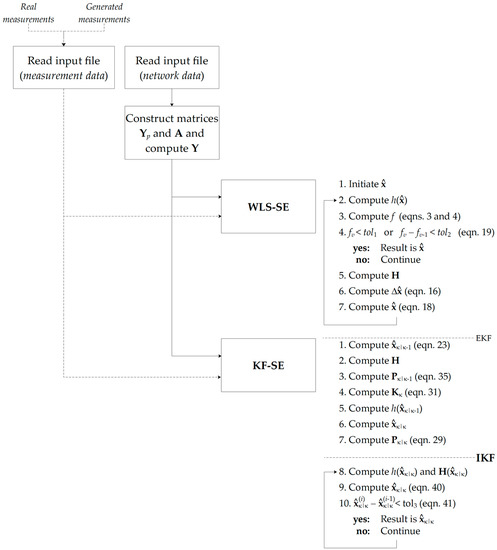
Figure 1. Three-phase state estimation algorithm.

The network data input file must contain the following information:

• For lines, sending and arriving nodes, line impedances, and shunt admittances;
• For transformers, sending and arriving nodes, rated voltages and power, and pu data;
• For shunt elements (e.g., capacitor banks), connection nodes, and rated voltage and power;
• States of circuit breakers.

The file containing the measurement data must contain all the measures obtained within the network:

• For loads and generating units, measurements of active and reactive powers, voltage magnitudes and phases, and current magnitudes;
• For lines, measurements of active and reactive transmitted powers, and current magnitudes.

The file may contain either real measures, obtained by smart meters and/or PMUs, or pseudo-measurements.

For the initialization of x in the three-phase WLS-SE algorithm, a flat start is usually implemented.

For the KF-SE algorithm, the following hypothesis was considered: It was assumed that the power system was steady under normal operating conditions, for which the predicted state was assumed to be equal to the last estimated state of the previous time-iteration [32]; i.e., (23) and (37) become:

$${\widehat{\mathbf{x}}}_{\kappa |\kappa -1}={\widehat{\mathbf{x}}}_{\kappa -1|\kappa -1},$$

(46)

and (39) becomes:

$${\mathbf{P}}_{\kappa |\kappa -1}={\mathbf{P}}_{\kappa -1|\kappa -1}+{\mathbf{Q}}_{\kappa -1}.$$

(47)

The KF-SE performs from the second time-iteration by assuming the last estimated state equal to the one resulting from the previous WLS-SE. The KF takes some iterations to satisfactorily track the system state.

3. The Low-Voltage Network

The network, shown in Figure 2, was an LV radial distribution network fed by a 15/0.4-kV transformer between buses 1 and 11. It was composed of 4 feeders containing 135 branches, 12 of which were single-phase, and the rest were three-phase. The network was equipped with 75 measurement points corresponding to 66 consumers, 6 producers, and 3 prosumers, for a total of 9 photovoltaic (PV) power plants. Each of these measurement points observed one or more points of delivery. The results illustrated hereafter are relevant to the buses denoted with red numbers in Figure 2.

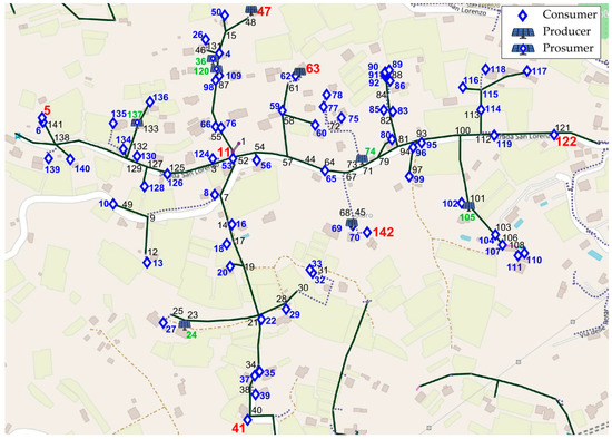
Figure 2. Topology of the observed low-voltage system with indication of the measurement points.

Meters sent voltages, active and reactive energy records, on a quarter-hourly basis, to the DMS developed in the PODCAST project. The voltage at the MV-side of the transformer in the main substation was considered constant and symmetric with a magnitude of 1 pu.

It was assumed that all the information arrived at the DMS without delays and all measures were time synchronized. The implications of such assumption were assessed further.

The performances of the implemented SE algorithms were assessed in a time horizon of 1 day. For the SE algorithm validation, the true values of the observed quantities were needed, so they were obtained by means of load flow calculations assuming realistic load and generation profiles. The active and reactive powers for the analyzed nodes are shown in Figure 3, and the voltage profiles in Figure 4. The maximum and minimum voltage values within the network are also reported in Figure 4.

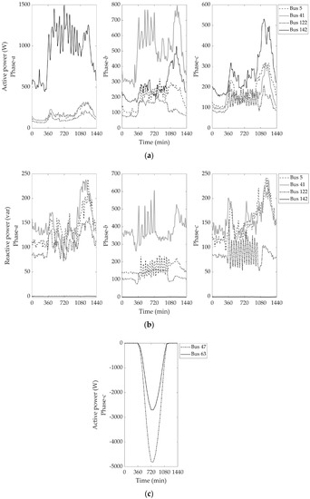
Figure 3. Power profiles of (a) active and (b) reactive consumption, and (c) PV production.

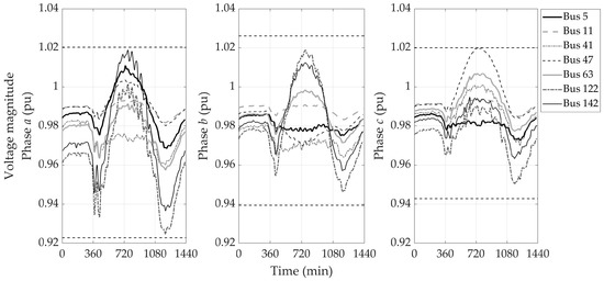
Figure 4. True values of the voltages of the analyzed nodes. The maximum and minimum values within the network are also illustrated.

The measured values were obtained by adding a measurement noise to the calculated power and voltage values. The measurement noise covariance matrix R was built by assuming the standard deviations indicated in Table 1 and considering the measurements errors uncorrelated.

Table 1. Measurement standard deviations.

Standard Deviations
Voltage magnitude—σE	0.653 V (0.2% of Emax)
Voltage phase angle—σδ	1 mrad
Power—σS	40 W (0.2% of 20 kW)

4. Test Results

For the appraisal of the performances of the developed methods, the average absolute deviation (aad) was calculated:

$$\mathit{aad}=\frac{1}{n}{\displaystyle \sum _{i=1}^n\left|{\dot{u}}_i-{\widehat{u}}_i\right|}$$

(48)

where ${\dot{u}}_i$ and ${\widehat{u}}_i$ are the true and estimated values of u at the i-th instant, and n is the number of samples, equal to 96 for the considered case.

As already mentioned, other than R, the performance of the KF-SE was strongly influenced by the process noise covariance matrix Q. The values of q_ang and q_mag, for which:

$$\mathbf{Q}=\mathrm{diag}(\underset{\frac{N}{2}-1}{\underbracket{q_{\mathit{ang}},\dots ,q_{\mathit{ang}}}},\underset{\frac{N}{2}}{\underbracket{q_{\mathit{mag}},\dots ,\hspace{0.17em}{q}_{\mathit{mag}}}}).$$

(49)

were chosen by analyzing the values of aad for different values of q in a 1-week dataset, as done in [33]. The resulting optimized values were 6.5 × 10⁻⁴ and 3 × 10⁻⁵, respectively.

4.1. Base Case

The estimated states of the analyzed nodes, on a quarter-hourly basis, with both the WLS and the KF-SE methods are reported in Figure 5, Figure 6 and Figure 7. To avoid the influence of the KF initialization errors mentioned in Section 2.4, the SE algorithms were initialized a half-day before.

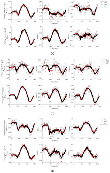
Figure 5. Estimated state values at buses (a) 5, (b) 11, and (c) 41.

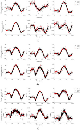
Figure 6. Estimated state values at buses (a) 47, (b) 63, and (c) 122.

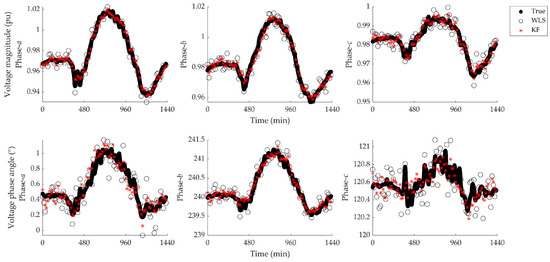
Figure 7. Estimated state values at bus 142.

The aad values for each node for both SE methods are reported in Figure 8, and their total values in Table 2. The improvement with respect to typical arbitrary values of q is also shown. Relative changes are reported with respect to the WLS-SE.

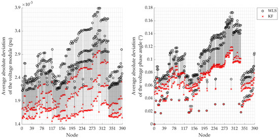
Figure 8. Average absolute deviation values for each node.

Table 2. Total average absolute deviations for different SE methods.

	WLS-SE	KF-SE
		qi = 1 × 10−6	qi = 1 × 10−5	qi = 1 × 10−4	qmag = 6.5 × 10−4 qang = 3.0 × 10−5 (Optimized)
aad (magnitude)	2.68 × 10−3	7.50 × 10−3	5.66 × 10−3	2.74 × 10−3	1.92 × 10−3 (−28.4%)
aad (phase angle)	0.095	0.108	0.077	0.077	0.070 (−25.9%)

4.2. Influence of Measurement Nonsynchronicity and Time Delays

The above results were obtained under the assumption that all the network data were collected by the DMS and processed instantaneously, and that the timestamps were coincident. Actually, smart meters transmit data to the DMS with delays that can be very large depending on the advanced metering infrastructure technology [24,34].

The results below consider the case of nonsynchronized data transmitted by the distributed measurement system. The scheme of Figure 9 elucidates the meaning of the considered time delays, in which t_n represents the time between consecutive measurements for the same node, t_m is the time elapsed between the time of the last state estimate and the arrival of the record, and t_del is the time delay elapsed from the measurement and its collection by the DMS. The nonsynchronicity was expressed by using t_m,i and t_del,i multiples of 30 s. The SE was carried out every 15 min, and all the measurements arriving after the last SE were used in the next SE, as represented by the red lines.

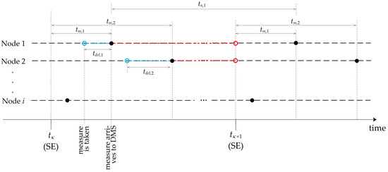
Figure 9. Nonsynchronicity between measurements.

Two scenarios were considered: (i) Scenario A: the measurements of each node were not synchronized, but arrived exactly every 15 min, i.e., all delays were null, t_n,i = 15 min, and t_m,i was constant but different for the various nodes; (ii) Scenario B: the measurements of each node were carried out every 15 min, but their arrival to the DMS was delayed by t_del, which randomly varied between 0 and t_max min. In this case, t_n,i and t_m,i were no longer constant. In some cases (mainly when t_n + t_m > 30 min) the delays were so large as to cause the SE to be computed without the updated information for some nodes.

First, simulations were carried out while considering a very accurate measurement dataset to highlight the influence of the nonsynchronicity and the time delays on the SE performance. The results obtained with only the KF-SE algorithm are reported in Figure 10, together with those obtained under the assumption of measurement synchronicity without delays, i.e., the ideal case.

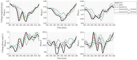
Figure 10. Estimated state values at node 122 considering data nonsynchronicity and time delays.

Finally, simulations were repeated considering the nonsynchronicity and the measurement standard deviations in Table 1. The resulting aad values obtained with both SE algorithms are reported in Table 3. Relative variations are reported with respect to the ideal case. From the obtained results, it was concluded that the influence of nonsynchronicity and time delays were moderate if they were restrained within some limits, e.g., one period of the SE computation. As time delays became larger, the worsening performance of the SE computation became significant.

Table 3. Total average absolute deviations considering data nonsynchronicity and time delays.

	WLS-SE
	Ideal	Asynchronous (Scenario A)	Asynchronous (Scenario B)
aad (magnitude)	2.68 × 10−3	2.73 × 10−3 (+2.0%)	tmax = 15 min	tmax = 60 min
			3.08 × 10−3 (+14.8%)	3.43 × 10−3 (+27.8%)
aad (phase angle)	0.095	0.098 (+3.4%)	tmax = 15 min	tmax = 60 min
			0.107 (+13.1%)	0.117 (+23.7%)
	KF-SE
	Ideal	Asynchronous (Scenario A)	Asynchronous (Scenario B)
aad (magnitude)	1.92 × 10−3	2.10 × 10−3 (+9.4%)	tmax = 15 min	tmax = 60 min
			2.39 × 10−3 (+24.4%)	2.94 × 10−3 (+53.1%)
aad (phase angle)	0.070	0.073 (+3.8%)	tmax = 15 min	tmax = 60 min
			0.078 (+11.1%)	0.085 (+21.2%)

5. Conclusions and Future Development

The implementation of a state estimation (SE) algorithm in a real low-voltage network has been presented. Two common methods for the SE computation were implemented and compared, mainly the weighted least squares (WLS) and the iterated Kalman filter (KF). The algorithms could consider unbalanced networks, as well as real load and generation profiles.

Due to the fluctuating nature of loads and of distributed generation, the resulting voltage profile fluctuates as well, for which the KF parameters, in particular the process noise covariance matrix, must be carefully tuned. The selection of the KF parameters was carried out on a 1-week dataset, and the advantages of applying such a procedure with respect to the adoption of typical values selected a priori were illustrated.

The comparison between both SE algorithms showed the improvement obtained by the KF implementation in terms of average absolute deviation of the voltage magnitudes and phase angles. For the analyzed scenario, the KF implementation led to reductions of the average absolute deviations of 28.4% and 25.9% for the estimated voltage magnitudes and phase angles, respectively.

The influences of the measurements’ nonsynchronicity and of the process and/or communication delays were quantified and analyzed. The influence of measurement nonsynchronicity when delays were not considered was very limited. In such a scenario, the average absolute deviations increased 2.0% and 9.4% for the estimated voltage magnitudes and 3.4% and 3.8% for the estimated voltage phase angles, with WLS and KF-SE, respectively. The influence of time delays depended on their size. If the delays were limited, e.g., within one period of the SE computation, the deviations increased 14.8% and 24.4% for the voltage magnitudes and 13.1% and 11.1% for the voltage phase angles, with WLS and KF-SE, respectively. As time delays became larger, the performance of the SE computation worsened significantly. For instance, for the scenario in which delays could reach 1 h, the deviations increased 27.8% and 53.1% for the voltage magnitudes and 23.7% and 21.2% for the voltage phase angles, depending on whether the WLS or the KF-SE was implemented, respectively.

The KF-SE also constituted a valid approach for distribution networks equipped predominantly with smart meters, providing a low measurement rate and in the presence of renewable energy sources such as photovoltaic power plants. Future work should aim at optimizing the value of the prediction covariance matrix, for which adaptive strategies might be appropriate, particularly in the presence of unpredictable energy production or load variations. Moreover, further strategies must be developed to mitigate the effect of measurement nonsynchronicity and time delays on the robustness of SE.

References

- Vaahedi, E. Practical Power System Operation; El-Hawary, M., Ed.; John Wiley & Sons Inc.: Hoboken, NJ, USA, 2014; ISBN 9781118915110. [Google Scholar]
- Primadianto, A.; Lu, C.N. A Review on Distribution System State Estimation. IEEE Trans. Power Syst. 2017, 32, 3875–3883. [Google Scholar] [CrossRef]
- Abur, A.; Expósito, A.G. Power System State Estimation: Theory and Implementation; CRC Press: Boca Raton, FL, USA, 2004; ISBN 0203913671. [Google Scholar]
- Zhao, J.; Gómez-Expósito, A.; Netto, M.; Mili, L.; Abur, A.; Terzija, V.; Kamwa, I.; Pal, B.; Singh, A.K.; Qi, J.; et al. Power System Dynamic State Estimation: Motivations, Definitions, Methodologies, and Future Work. IEEE Trans. Power Syst. 2019, 34, 3188–3198. [Google Scholar] [CrossRef]
- Zanni, L. Power-System State Estimation Based on PMUs: Static and Dynamic Approaches—From Theory to Real Implementation; École Polytechnique Fédérale de Lausanne: Lausanne, Switzerland, 2017. [Google Scholar]
- Blood, E.A.; Krogh, B.H.; Ilić, M.D. Electric power system static state estimation through Kalman filtering and load forecasting. In Proceedings of the IEEE Power and Energy Society 2008 General Meeting: Conversion and Delivery of Electrical Energy in the 21st Century, PES, Pittsburgh, PA, USA, 20–24 July 2008. [Google Scholar]
- Sarri, S.; Paolone, M.; Cherkaoui, R.; Borghetti, A.; Napolitano, F.; Nucci, C.A. State estimation of Active Distribution Networks: Comparison between WLS and iterated kalman-filter algorithm integrating PMUs. In Proceedings of the 3rd IEEE PES Innovative Smart Grid Technologies Conference Europe, Berlin, Germany, 14–17 October 2012. [Google Scholar]
- Sarri, S.; Zanni, L.; Popovic, M.; Le Boudec, J.Y.; Paolone, M. Performance Assessment of Linear State Estimators Using Synchrophasor Measurements. IEEE Trans. Instrum. Meas. 2016, 65, 535–548. [Google Scholar] [CrossRef]
- Brüggemann, A.; Görner, K.; Rehtanz, C. Evaluation of extended Kalman filter and particle filter approaches for quasi-dynamic distribution system state estimation. CIRED Open Access Proc. J. 2017, 1, 1755–1758. [Google Scholar] [CrossRef][Green Version]
- Valverde, G.; Terzija, V. Unscented Kalman filter for power system dynamic state estimation. IET Gener. Transm. Distrib. 2011, 5, 29–37. [Google Scholar] [CrossRef]
- Zhou, N.; Huang, Z.; Li, Y.; Welch, G. Local sequential ensemble Kalman filter for simultaneously tracking states and parameters. In Proceedings of the 2012 North American Power Symposium, NAPS 2012, Champaign, IL, USA, 9–11 September 2012. [Google Scholar]
- Dehghanpour, K.; Wang, Z.; Wang, J.; Yuan, Y.; Bu, F. A Survey on State Estimation Techniques and Challenges in Smart Distribution Systems. IEEE Trans. Smart Grid 2019, 10, 2312–2322. [Google Scholar] [CrossRef]
- Ahmad, F.; Rasool, A.; Ozsoy, E.; Sekar, R.; Sabanovic, A.; Elitaş, M. Distribution system state estimation-A step towards smart grid. Renew. Sustain. Energy Rev. 2018, 81, 2659–2671. [Google Scholar] [CrossRef]
- Durgaprasad, G.; Thakur, S.S. Robust dynamic state estimation of power systems based on M-Estimation and realistic modeling of system dynamics. IEEE Trans. Power Syst. 1998, 13, 1331–1336. [Google Scholar] [CrossRef]
- Mestav, K.R.; Luengo-Rozas, J.; Tong, L. Bayesian State Estimation for Unobservable Distribution Systems via Deep Learning. IEEE Trans. Power Syst. 2019, 34, 4910–4920. [Google Scholar] [CrossRef]
- Zamzam, A.S.; Sidiropoulos, N.D. Physics-Aware Neural Networks for Distribution System State Estimation. IEEE Trans. Power Syst. 2020, 35, 4347–4356. [Google Scholar] [CrossRef]
- Zhang, L.; Wang, G.; Giannakis, G.B. Real-Time Power System State Estimation and Forecasting via Deep Unrolled Neural Networks. IEEE Trans. Signal Process. 2019, 67, 4069–4077. [Google Scholar] [CrossRef]
- Gahrooei, Y.R.; Khodabakhshian, A.; Hooshmand, R.-A. A New Pseudo Load Profile Determination Approach in Low Voltage Distribution Networks. IEEE Trans. Power Syst. 2018, 33, 463–472. [Google Scholar] [CrossRef]
- Wang, Y.; Sun, Y.; Dinavahi, V. Robust Forecasting-Aided State Estimation for Power System Against Uncertainties. IEEE Trans. Power Syst. 2020, 35, 691–702. [Google Scholar] [CrossRef]
- Kong, X.; Zhang, X.; Zhang, X.; Wang, C.; Chiang, H.-D.; Li, P. Adaptive Dynamic State Estimation of Distribution Network Based on Interacting Multiple Model. IEEE Trans. Sustain. Energy 2021, 1. [Google Scholar] [CrossRef]
- Zhao, J.; Netto, M.; Mili, L. A Robust Iterated Extended Kalman Filter for Power System Dynamic State Estimation. IEEE Trans. Power Syst. 2017, 32, 3205–3216. [Google Scholar] [CrossRef]
- Mohammed, I.; Geetha, S.J.; Shinde, S.S.; Rajawat, K.; Chakrabarti, S. Modified Re-Iterated Kalman Filter for Handling Delayed and Lost Measurements in Power System State Estimation. IEEE Sens. J. 2020, 20, 3946–3955. [Google Scholar] [CrossRef]
- Paolone, M.; Le Boudec, J.-Y.; Sarri, S.; Zanni, L. Static and recursive PMU-based state estimation processes for transmission and distribution power grids. In Advances in Power System Modelling, Control and Stability Analysis; Milano, F., Ed.; The Institution of Engineering and Technology: London, UK, 2016; ISBN 978-1-78561-001-1. [Google Scholar]
- Alimardani, A.; Therrien, F.; Atanackovic, D.; Jatskevich, J.; Vaahedi, E. Distribution System State Estimation Based on Nonsynchronized Smart Meters. IEEE Trans. Smart Grid 2015, 6, 2919–2928. [Google Scholar] [CrossRef]
- Nainar, K.; Iov, F. Smart meter measurement-based state estimation for monitoring of low-voltage distribution grids. Energies 2020, 13, 5367. [Google Scholar] [CrossRef]
- Bessone, E.; Bianchi, S.; Massucco, S.; Nucci, C.A.; Pentolini, M.; Raco, F. The PODCAST project–optimizing distribution networks with renewable energy sources. In Proceedings of the 2018 AEIT International Annual Conference, Bari, Italy, 3–5 October 2018; pp. 1–6. [Google Scholar]
- Zhu, J.; Abur, A. Effect of Phasor Measurements on the Choice of Reference Bus for State Estimation. In Proceedings of the 2007 IEEE Power Engineering Society General Meeting, Tampa, FL, USA, 24–28 June 2007; pp. 1–5. [Google Scholar]
- Wang, S.; Zhao, J.; Huang, Z.; Diao, R. Assessing Gaussian assumption of PMU measurement error using field data. IEEE Trans. Power Deliv. 2018, 33, 3233–3236. [Google Scholar] [CrossRef]
- Sorenson, H.W. Least-Squares Estimation. From Gauss To Kalman. IEEE Spectr. 1970, 7, 63–68. [Google Scholar] [CrossRef]
- Gelb, A.; Kasper, J.F.; Nash, R.A.; Price, C.F.; Sutherland, A.A. Applied Optimal Estimation; Gelb, A., Ed.; The MIT Press: Cambridge, MA, USA; London, UK, 1974; ISBN 0-262-20027-9. [Google Scholar]
- Arrillaga, J.; Arnold, C.P. Computer Analysis of Power Systems; John Wiley & Sons Ltd.: Christchurch, New Zealand, 1990; ISBN 0-471-92760-0. [Google Scholar]
- Debs, A.S.; Larson, R.E. A Dynamic Estimator for Tracking the State of a Power System. IEEE Trans. Power Appar. Syst. 1970, PAS-89, 1670–1678. [Google Scholar] [CrossRef]
- Zanni, L.; Sarri, S.; Pignati, M.; Cherkaoui, R.; Paolone, M. Probabilistic assessment of the process-noise covariance matrix of discrete Kalman filter state estimation of active distribution networks. In Proceedings of the 13th International Conference on Probabilistic Methods Applied to Power Systems (PMAPS), Durham, UK, 7–10 July 2014. [Google Scholar]
- Kemal, M.; Sanchez, R.; Olsen, R.; Iov, F.; Schwefel, H.P. On the trade-off between timeliness and accuracy for low voltage distribution system grid monitoring utilizing smart meter data. Int. J. Electr. Power Energy Syst. 2020, 121, 106090. [Google Scholar] [CrossRef]
Publisher’s Note: MDPI stays neutral with regard to jurisdictional claims in published maps and institutional affiliations. |
© 2021 by the authors. Licensee MDPI, Basel, Switzerland. This article is an open access article distributed under the terms and conditions of the Creative Commons Attribution (CC BY) license (https://creativecommons.org/licenses/by/4.0/).