Wind Turbine Data Analysis and LSTM-Based Prediction in SCADA System

Abstract

The number of wind farms is increasing every year because many countries are turning their attention to renewable energy sources. Wind turbines are considered one of the best alternatives to produce clean energy. Most of the wind farms installed supervisory control and data acquisition (SCADA) system in their turbines to monitor wind turbines and logged the information as time-series data. It demands a powerful information extraction process for analysis and prediction. In this research, we present a data analysis framework to visualize the collected data from the SCADA system and recurrent neural network-based variant long short-term memory (LSTM) based prediction. The data analysis is presented in cartesian, polar, and cylindrical coordinates to understand the wind and energy generation relationship. The four features: wind speed, direction, generated active power, and theoretical power are predicted and compared with state-of-the-art methods. The obtained results confirm the applicability of our model in real-life scenarios that can assist the management team to manage the generated energy of wind turbines.

1. Introduction

Renewable energy sources are playing an important role in economic growth and are considered an alternative source of energy for environmental reasons. It can provide a clean and sustainable solution as compared to nonrenewable energy which heavily relies on coal, oil, and other fossil fuels [1,2]. The nonrenewable energy sources are not suitable due to global warming, which causes extreme weather events such as more frequent wildfires, droughts, heatwaves, melting of glaciers, and floods threatening our planet ecosystem [3]. Wind turbines are considered one of the primary sources of renewable energy generation that provides clean and sustainable energy in modern power systems. Furthermore, they are environment-friendly and have near to zero $C{O}_2$ emissions. The wind turbine based energy generation completely relies on the wind to keep it operational. However, wind speed and direction fluctuates [4,5]; therefore, the amount of energy produced may vary from one moment to another. It could be a severe setback since it is expected to be delivered and consumed on a real-time basis.

To manage the wind turbine, most wind farms have installed supervisory control and data acquisition (SCADA) systems for monitoring different components and logging the operational data [6,7]. This logged data contains information about wind speed, its direction, the amount of generated power, etc. It creates an opportunity to process the gathered time-series data for diverse applications ranging from operational and maintenance purposes to predictive analysis of generated energy by the wind turbines [8]. The analysis and prediction of energy generation can be beneficial for the management team who is managing the wind forms to make correct decisions about the generated power, its consumption, and prepare the storage capacity in smart grids.

The research community already developed statistical [9], machine learning [4], and artificial neural networks [10] based approaches for wind turbine prediction task. In this research, our aim is to perform an exploratory data analysis for a better understanding of the wind and generated power. The exploratory data analysis provides a deep insight into the wind turbine data logs by exploring available features, namely, wind speed, wind direction, active power, and theoretical power. Consequently, it will reduce the complexity of overall data logs to understand it. We designed a recurrent neural network variant long short-term memory (LSTM) model for wind turbines prediction. LSTMs can capture long-range dependencies and nonlinear dynamics given its internal structure. In this research, our contribution is as follows:

• To design and develop a unique visualization platform for the analysis of wind turbine data gathered by the SCADA system.
• To design and develop an efficient deep learning model for short term time-series prediction (with a time frame of a month).
• To perform a comparative analysis with existing statistical and machine learning approaches to measure the improvements.

The structure of the paper is as follows: Section 2 outlines the related work on SCADA systems with research studies to forecast the wind power. In Section 3.1, the exploratory data analysis is performed to visualize the collected SCADA datasets. The detail about recurrent neural network variant LSTM-based prediction is presented in Section 3.2, while Section 4 presents the implementation details, obtained results, and comparison followed by discussions. The paper is concluded in Section 5 with possible future directions.

2. Related Works

Wind farms are attached to the SCADA system to constantly collect data about wind turbines. This data can be utilized for different analysis including failure prediction [8], gearbox malfunction [7], assessment of the wind turbine performance [11], and wind-turbine wake effect [12,13,14]. There have been many research studies to forecast wind power according to the characteristics of wind farms. In the wind power industry, neural networks are intensively being used to generate accurate predictions or for comparison purposes with the classical forecasting methods. In the early days, Xiaodan et al. [9] developed a statistical method to forecast the short-term wind power in one wind farm in western China. Their method is based on Autoregressive and Moving Average (ARMA) and satisfactory results are reported in terms of absolute error average. In case of strong randomness of wind speed, their model is less accurate.

Sun et al. [15] considered the artificial neural network (ANN) is developed to model the power of wind turbines. In their network training, they also considered the wake effect based on geographic and wind-turbine information. Their study concludes that wind turbines in different positions should adopt different yaw angle control strategies. A recurrent neural network variant LSTM [16] can learn the time-series information more effectively. It has the power to utilize temporal information efficiently for forecasting the new data points. It is successfully used in stock market predictions [17], natural language processing [18], and also in medicine [19].

In wind power energy, Alencar et al. [10] develops ultra-short, short, medium, and long term prediction models of wind speed prediction. They utilized the Autoregressive Integrated Moving Average (ARIMA), artificial neural network, and hybrid models. The experiments were performed on the dataset obtain in Brazil by the national organization system of environmental data (SONDA). They achieved better results in the case of the hybrid model and reported neural network based models are better than statistical methods like ARMA and ARIMA. Similarly, Khosravi et al. [4] applied machine learning algorithms to predict the wind speed for Osorio wind farm in the south of Brazil. They applied neural networks, support vector regression, fuzzy inference system optimized with computational intelligence-based algorithms. They reported a neural network based model outperform as compared to the considered model in the study. Furthermore, they conclude wind speed has a direct influence on the generated power.

Liu et al. [20] developed a short-term prediction of wind power that is based on discrete wavelet transform and LSTM. Their study concludes that LSTM based model can effectively capture the dynamic behavior of wind energy. Furthermore, they also decomposed the nonstationary time series data using discrete wavelet transformation. After transformation, they consider each component as independent and temporal relations were learned by LSTM. The comparison results proved superior results as compared to the recurrent neural network, multilayered feed-forward neural networks with backpropagation, and combination with discrete wavelet transformation. Similarly, Han et al. [21] developed a short-term wind prediction model based on LSTM for Jeju island in South Korea. They have a vision for realizing carbon free Jeju by 2030.

In previously developed models, the visualization of time-series data logs are missing which can help the management team to understand and analyze the unseen problems. Our research focused on the visualization and the prediction aspect of wind energy generation. The proposed framework provides short-term data visualization (i.e., time-stamp of one month), and it has the ability to predict the wind and energy generation that may help to manage smart grids.

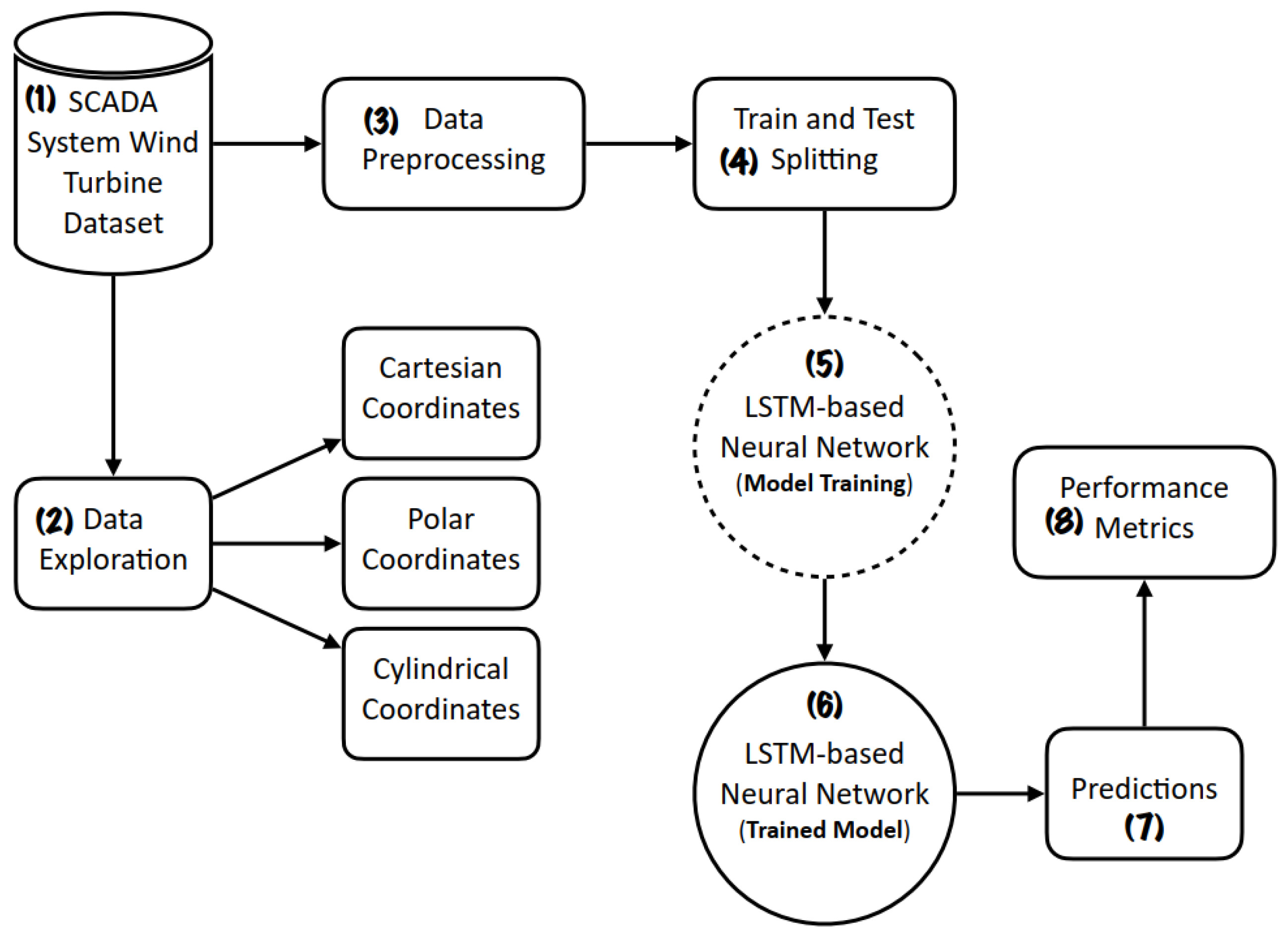
3. The Proposed Model

The proposed model is illustrated in Figure 1 and it consists of: (a) exploratory data analysis; and (b) the prediction. The details of the subcomponents are as follows.

3.1. Exploratory Data Analysis

The exploratory data analysis is performed using visualization techniques. It can provide a better understanding about the data logs of SCADA system of wind turbines. The details are provided in the following subsections.

3.1.1. Dataset

The data analysis and prediction is performed over the publicly available dataset that is collected in the northwestern region of Turkey [22]. The onshore wind farm is monitored by the SCADA system to capture the information about the wind and power generation properties of the Yalova region. The measurements were made as time-series data which logs the information at the interval of ten-minutes during the year 2018. It contains four measurements. (1) Active power: it provides data about the power generated by the wind turbine. (2) Wind speed: it measures the speed at the hub height of the turbine. (3) Wind direction: It logs the direction of the turbine that turns automatically to the direction where the wind blows (4) Theoretical power: it is the power value computed by the control system using the current wind speed. It is computed by using wind speed related to kinetic energy (i.e., Equation (3)). One week readings are presented in Figure 2.

In Figure 2, theoretical and active power is measured in terms of kilo watt $\left(kw\right)$, wind speed in meters per second (m/s), and its direction in degrees (∘). The x-axis presents time over the interval of 10 min, while the y-axis presents the unit for each feature of the SCADA system.

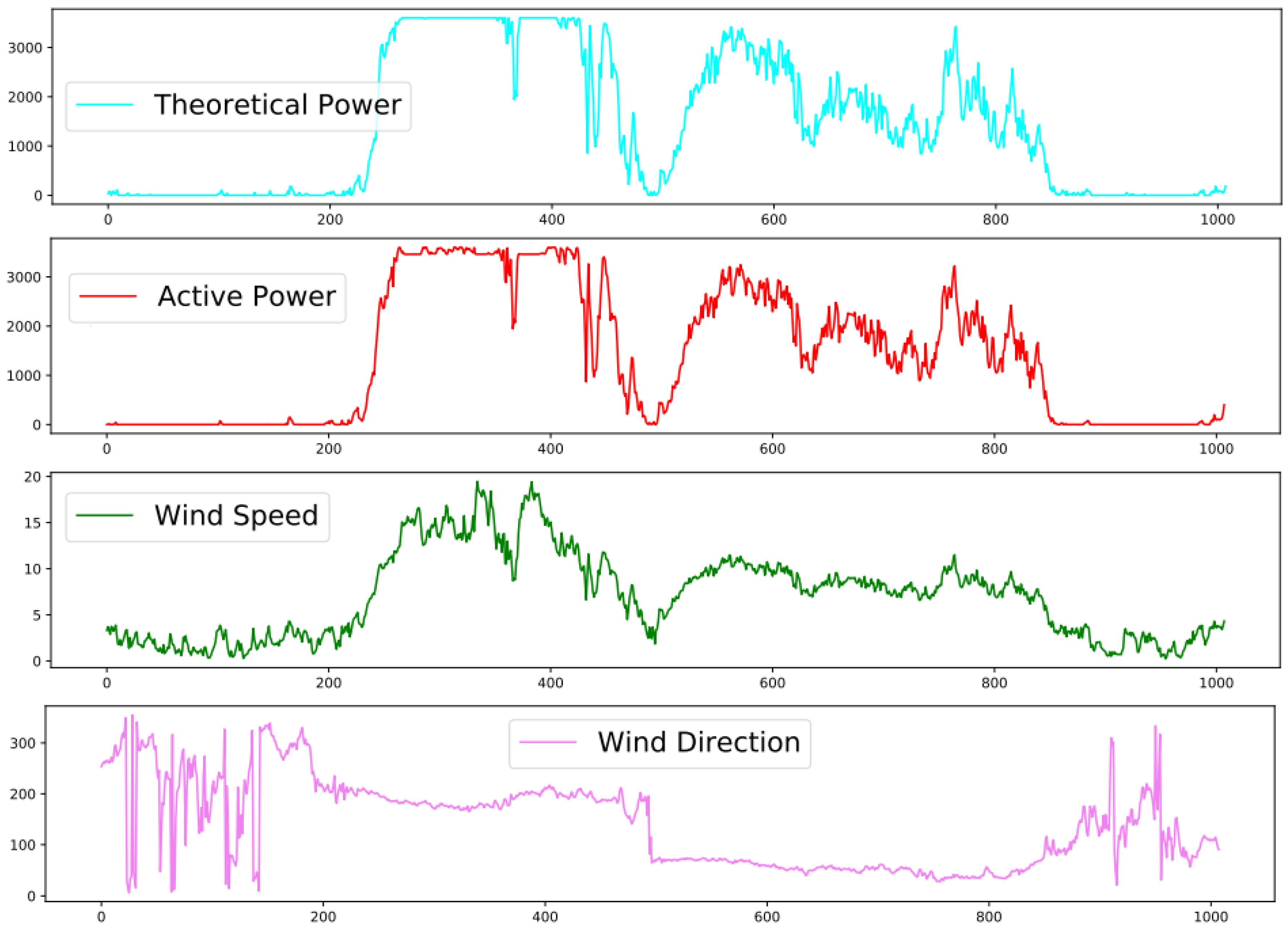
3.1.2. Data Analysis

The time-series data is transformed into a visual representation, where all its characteristics and distinguishable elements are clearly noticeable. It can provide useful information and assists the management team to understand the possible issues. Figure 3 presents data visualization with possible analysis factors.

In Figure 3, it can be seen that regions where the wind blows the most, model corroboration in terms of actual energy generation with theoretical power curve, the anomalies, and wind behavior in terms of speed and direction. The following section provides the details about each visualization generation and explanation:

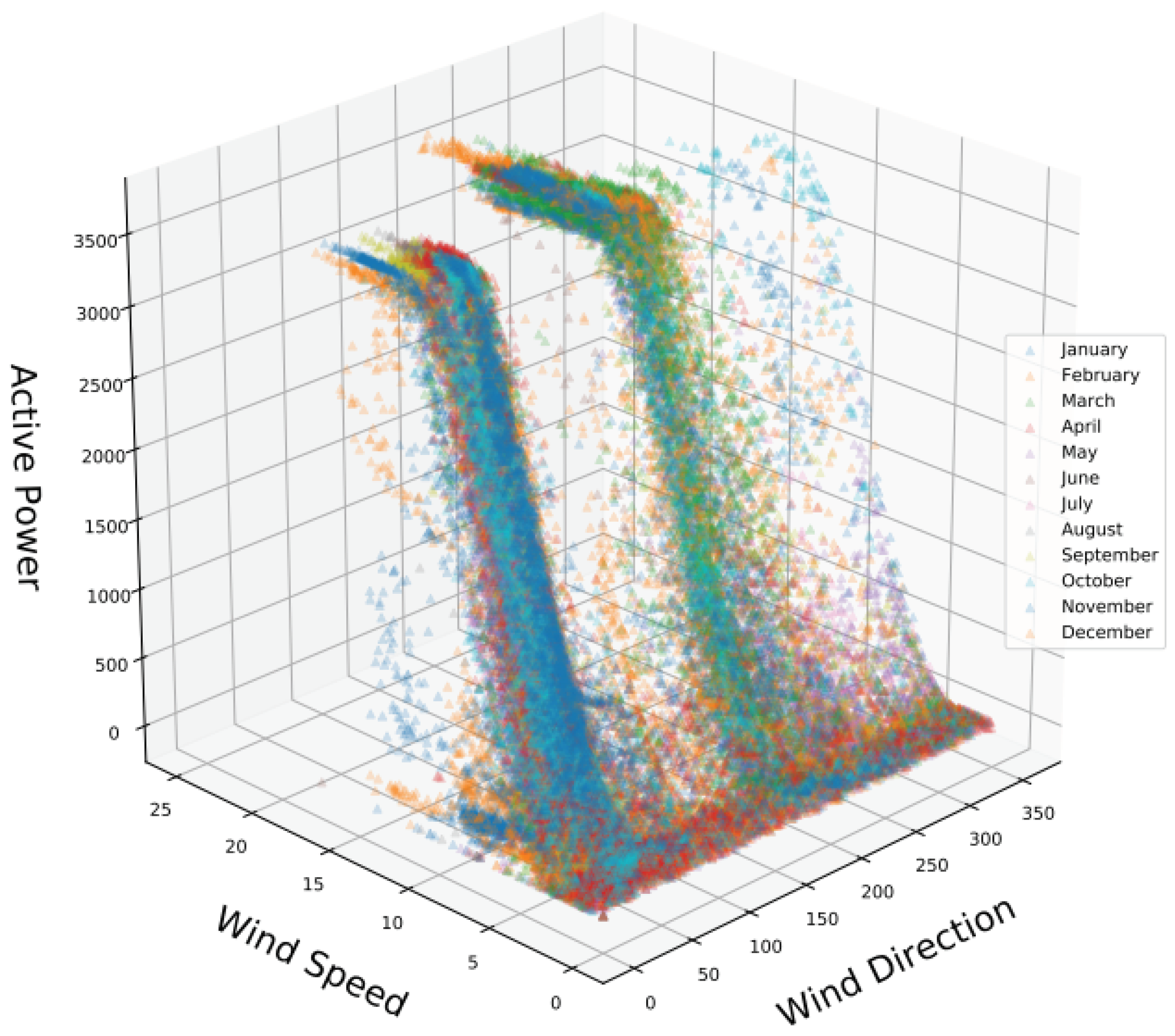
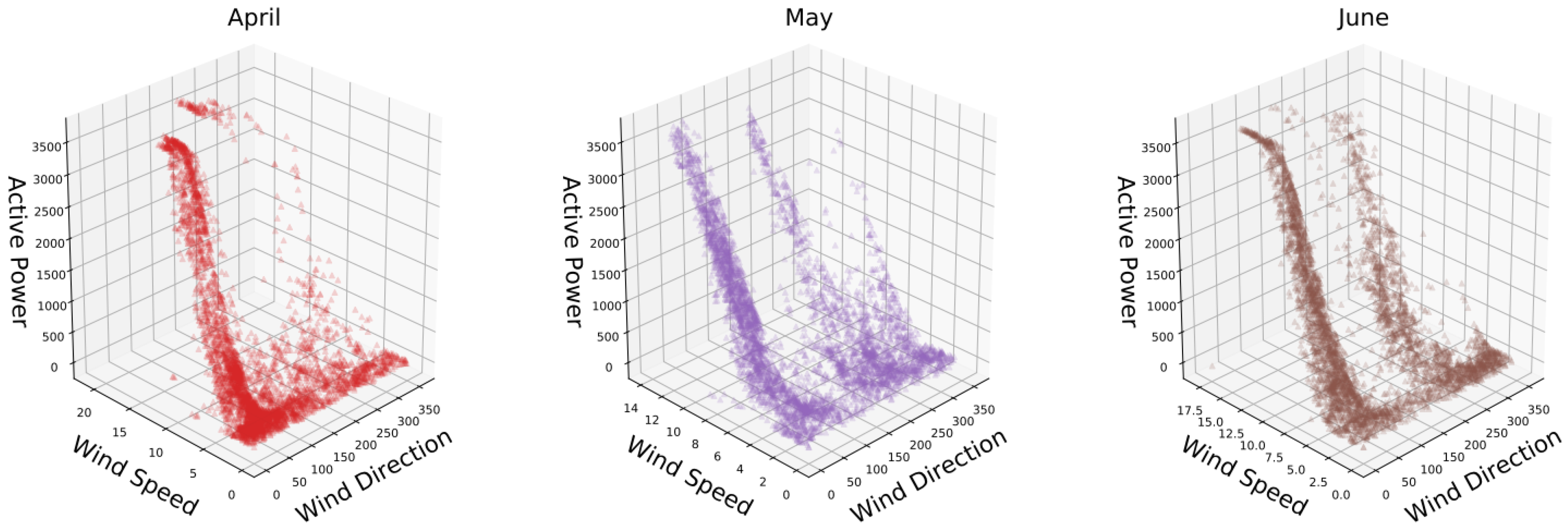
3.1.3. Cartesian Coordinates Analysis

The wind speed and direction can play an important role in analyzing the generated power. Although the wind direction determines the regions where the wind blows over a certain area and the wind speed determines the amount of power to be produced. Given the wind speed cubic relation (i.e., shown in Equation (3)) with the generated power, the higher the wind speed the more power is to be expected. In the Cartesian coordinates system, a three-dimensional space is considered that is based on three perpendicular axes (i.e., Wind speed, direction, and generated active power). In Figure 4, it presents a three dimensional data visualization for the whole year.

In Figure 4, two regions are dense that contribute maximum power generation. First region can be observed between $[{50}^{\circ }\sim {100}^{\circ }]$, while second region is around $[{200}^{\circ }\sim {250}^{\circ }]$ along wind direction. In the case of wind speed, it starts generating active power when the wind is blowing more than 5 m/s. Furthermore, the whole year is nearly consistent with the same wind behavior. It can be observed by visualizing every month to understand the concentrated regions, as shown in Figure 5.

In Figure 5, every month shows a nearly consistent pattern for wind direction as well as speed.

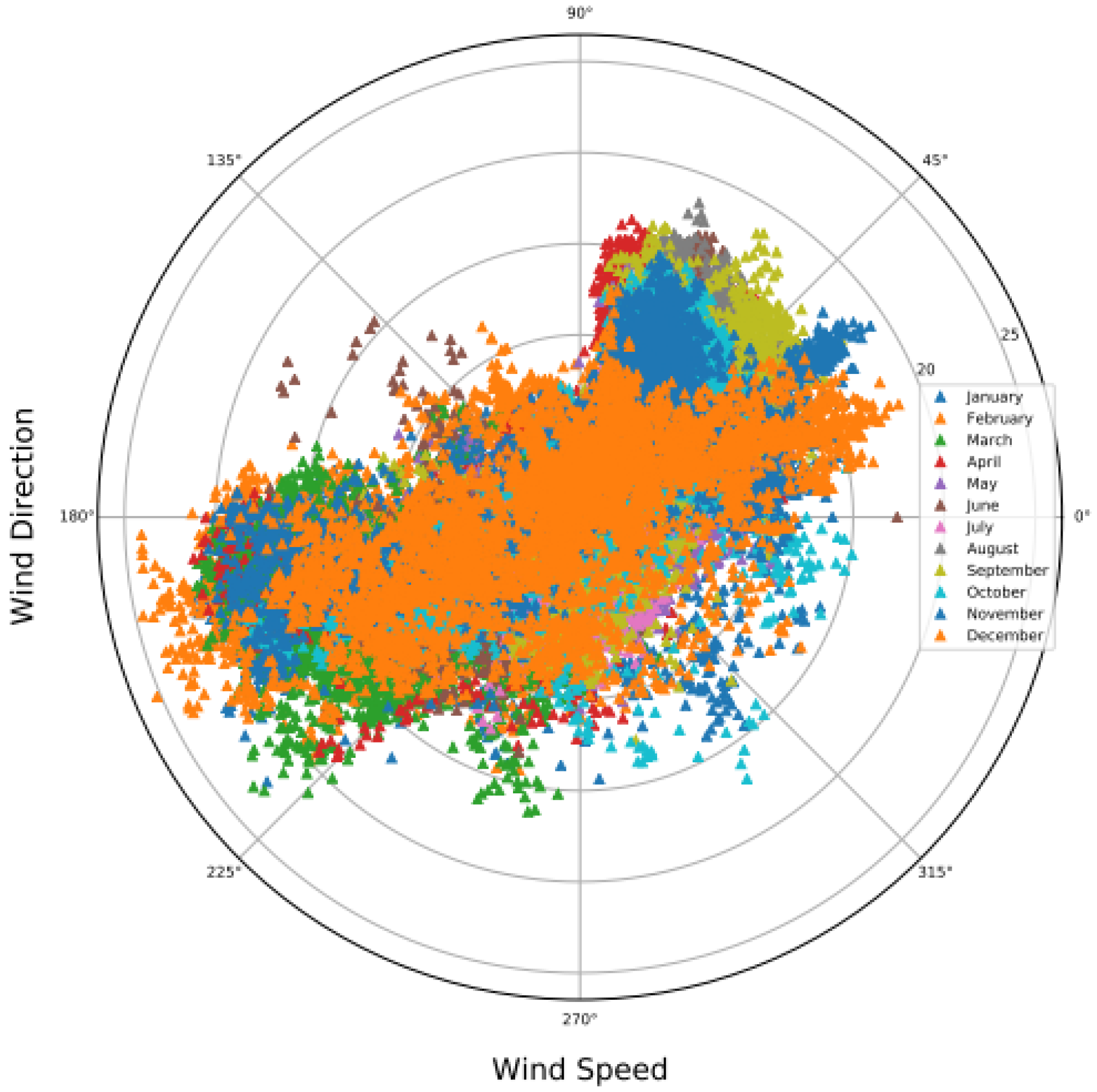
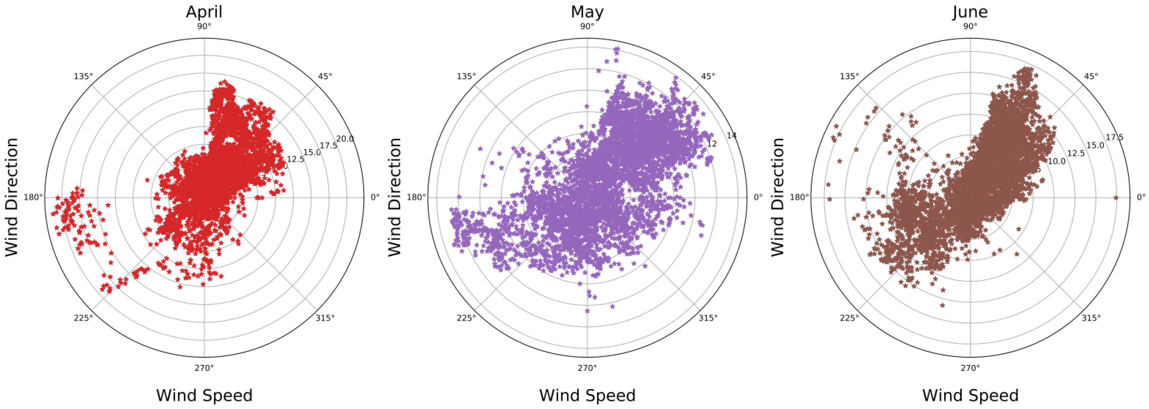
3.1.4. Polar Coordinates Analysis

In polar coordinates, the compass rose is used as a base model to identify the most active regions where the wind blows. The following Figure 6 presents the whole year’s wind direction and speed.

In Figure 6, the observation can be made that wind blows northeast and southwest along with the wind speed that is observed over the diameter of polar coordinates. The individual patterns for the month of April, May, and June are presented in Figure 7.

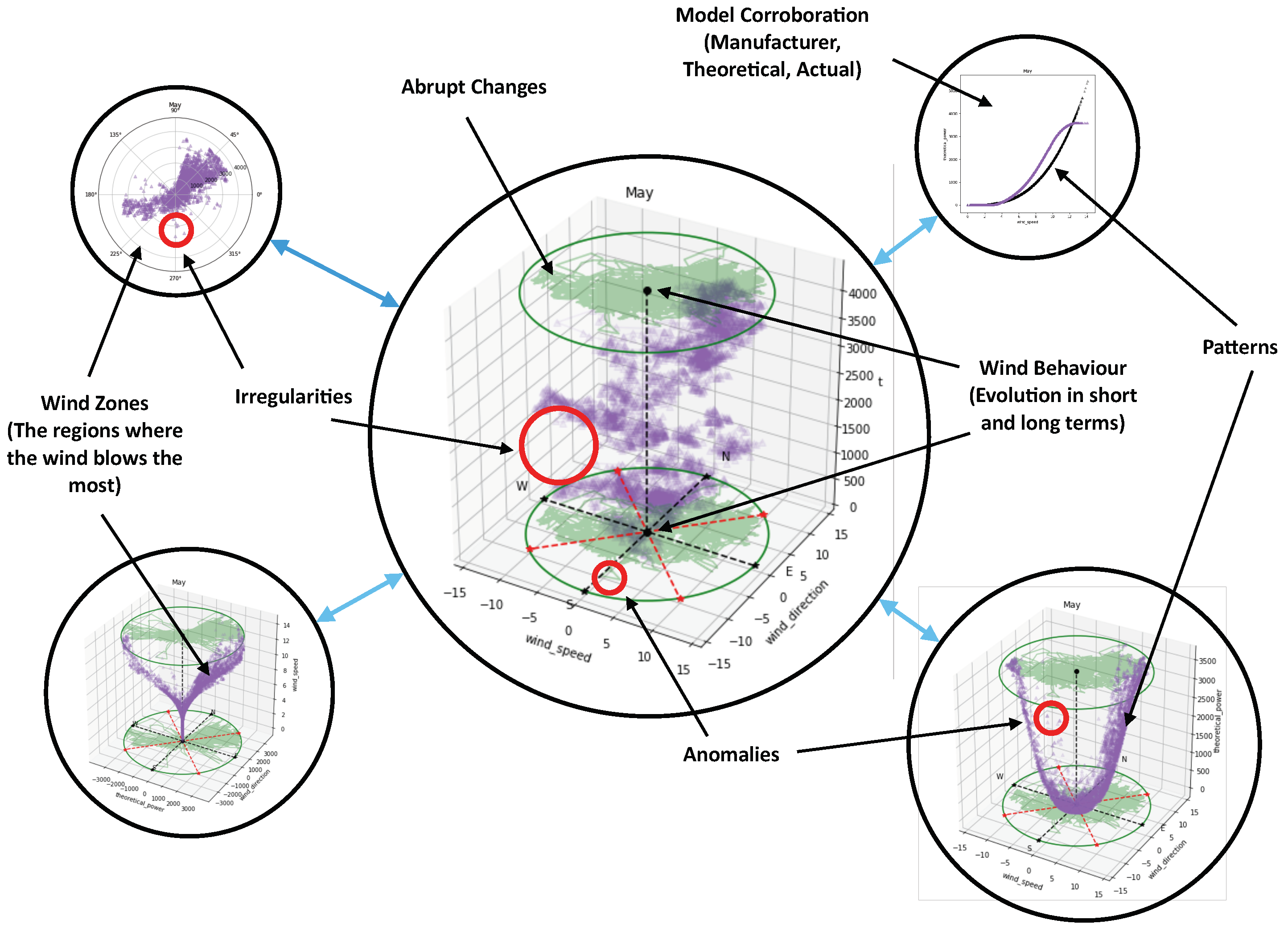
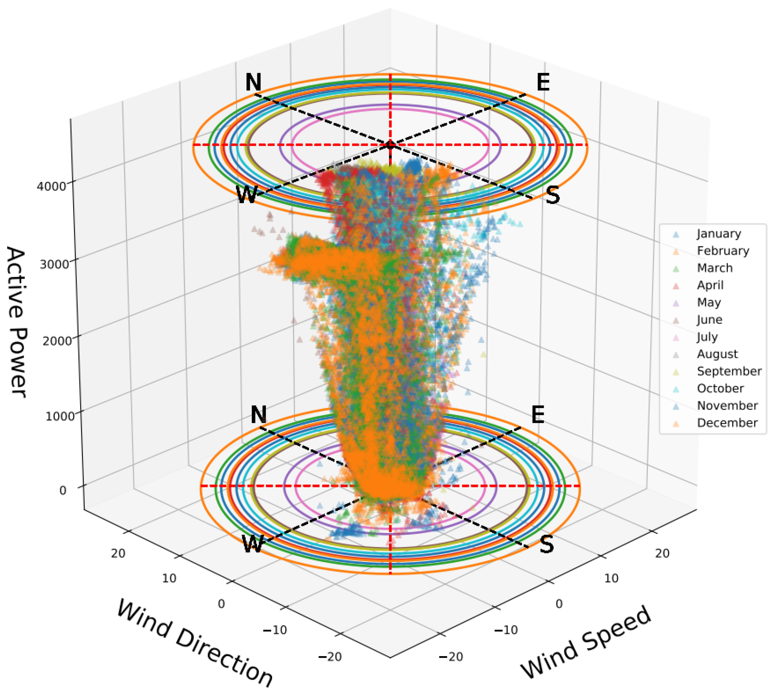
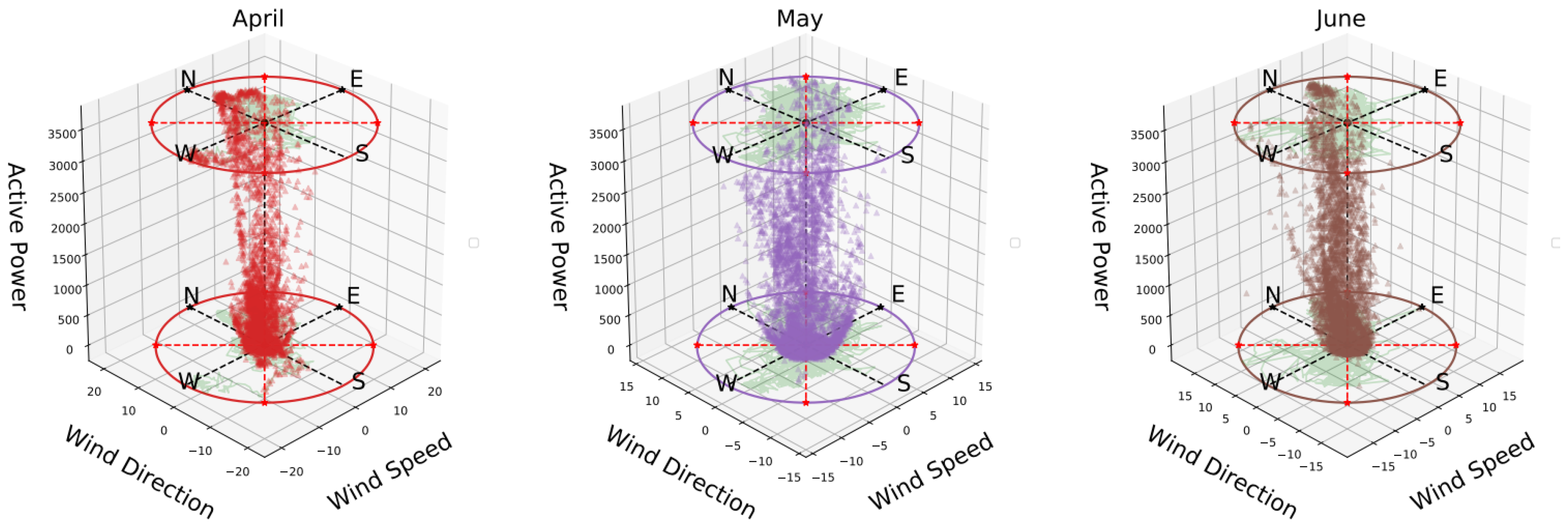
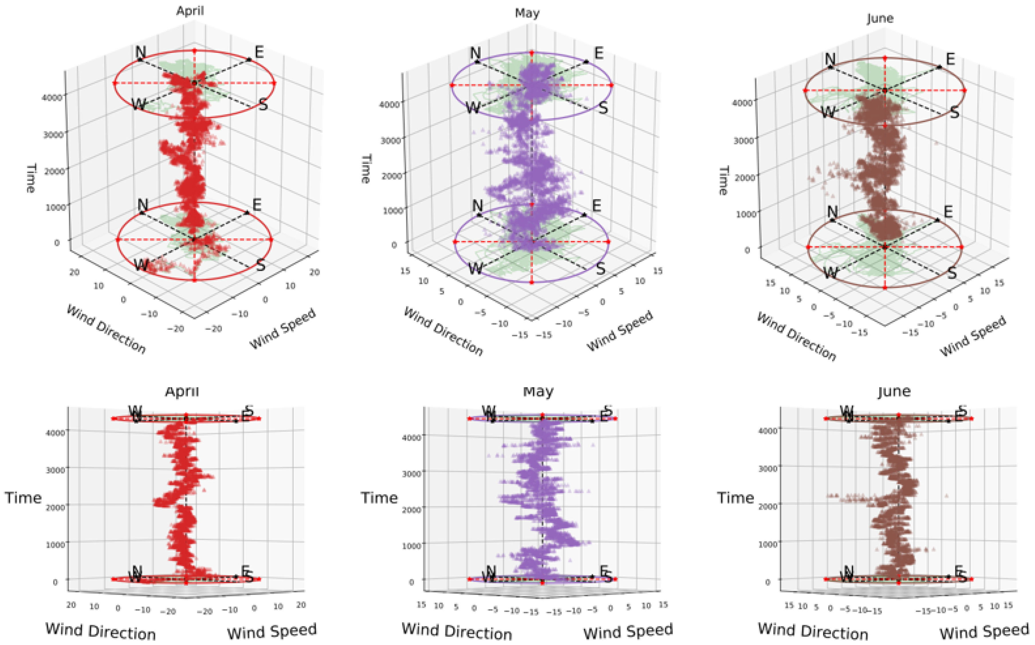
3.1.5. Cylindrical Coordinates Analysis

In cylindrical coordinates, visualization may assist in knowing the generated power for a given wind speed and direction. In Figure 8, the information is compact with compass rose model and each month is presented by the circle. The radius of the circle represents the maximum speed of the wind for that specific month.

For instance, wind behavior can be tracked by visualizing its footprint by evolving it through time as a new dimension. It can report the major changes in the wind for the region as well as point out where the changes start and where they continue as shown in Figure 9.

Figure 9 provides the information about the wind behavior at different moments between the active regions where the wind is blowing, these regions are displayed as the wind footprints in green for every month. Similarly, in Figure 10, the wind speed and direction is evolved with time for the month of April, May, and June. Every month shows some irregularities at a certain level, for example, almost at the middle of the considered month a small change happens with the wind speed. This pattern in the month of April shows a low wind speed value, then it starts to smoothly increase nearly half of the month later. Similarly, in the month of May, the wind speed is greater in the second part of the month, and in the month of June, an unusual change can be seen almost at the middle of the month in the wind speed value.

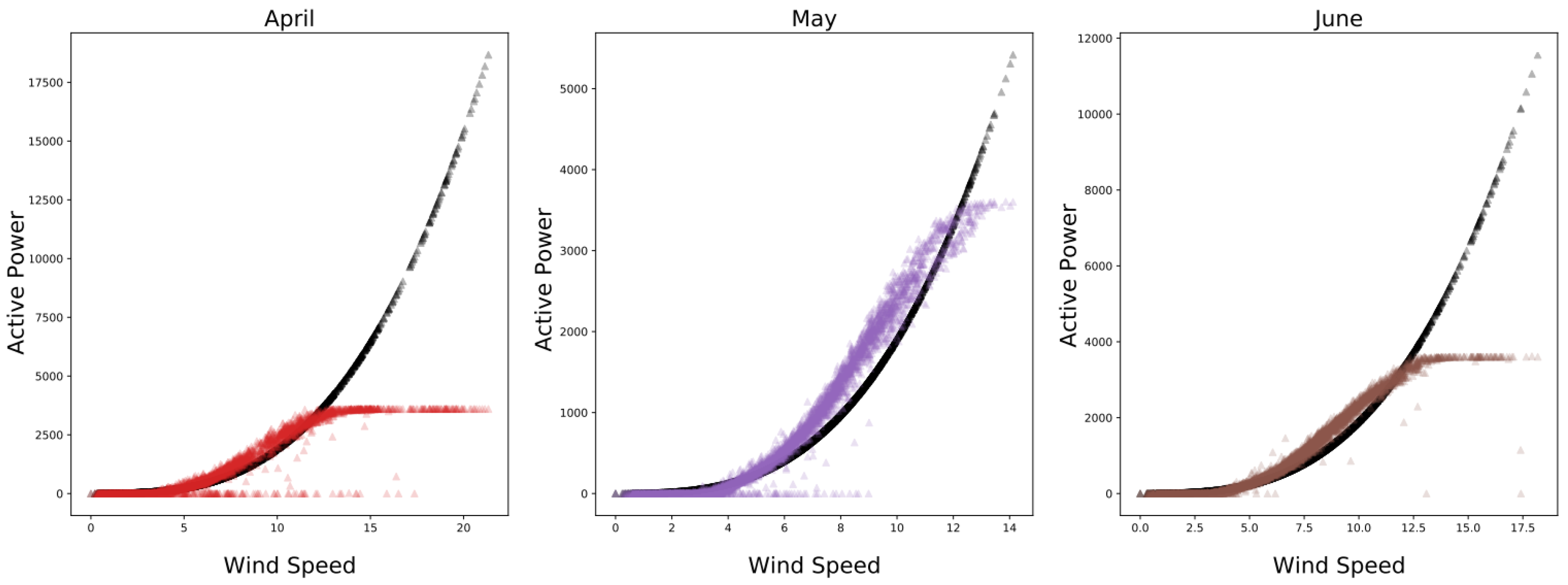
3.1.6. Wind Energy Generated Patterns

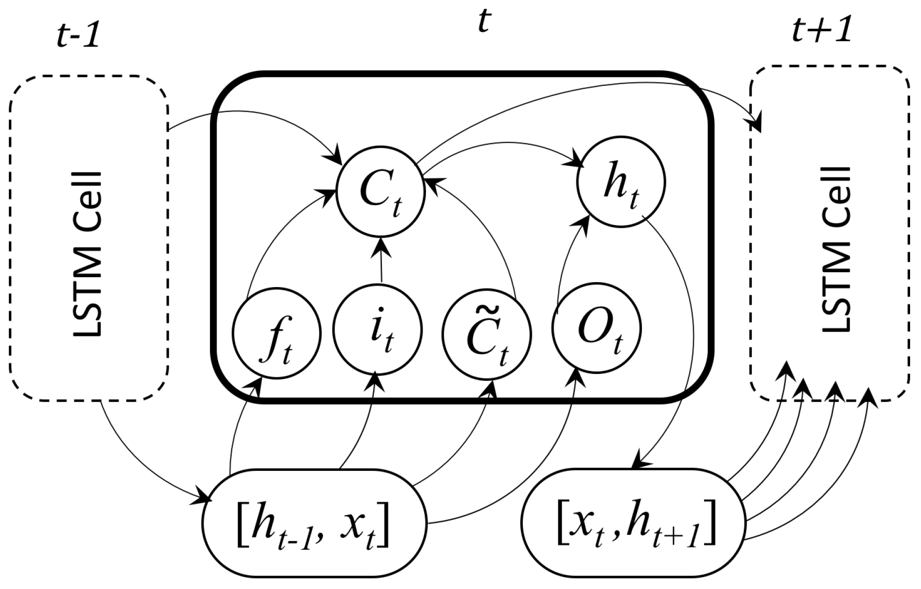
The dynamical behavior of the wind is related to the basics of its kinetic energy. The drawback is an energy generation system is always less than 100%, which means that we cannot transform one form of energy into another without loss. The entire energy generated by the wind turns out that nearly 59% of it can be transformed into power. This fact is known as the Betz limit [23] and it is independent of the turbine model. The theoretical power can be calculated by wind speed and it is related to the basics of its kinetic energy. It can be defined as:

$$k_e=\frac{1}{2}m{v}^2$$

(1)

The wind consists of a lot of tiny particles, each one having kinetic energy; however, it is difficult to count every single particle. In order to obtain the kinetic energy, instead the mass flow of all those particles going towards and through the wind turbine area is used. This particle mass flow is defined as the density of the air $\rho$ times the swept area of the turbine A times the velocity of the air v, i.e.,

$$\frac{dm}{dt}=\rho Av$$

(2)

By substituting Equation (2) in kinetic energy, we get:

$$P_w=\frac{1}{2}\rho A{v}^3$$

(3)

The theoretical power is computed by Equation (3), and it is plotted into Figure 11 with active power generated by wind turbine for the month of April, May, and June.

In Figure 11, the active power generated by the wind turbine follows nearly the same relation that is defined by the Betz limit. While in the case of April the generated power is even lower than 59%, which shows some external factors also contribute—this can be tuned to get the maximum output from the wind turbine.

3.2. The Prediction

Let us consider univariate time-series data and represent each feature as f. It can be defined as:

$$f:\left\{x_0,x_1,x_2,\dots x_{s-2},x_{s-1},x_s\right\}.$$

(4)

where subindex s represents the number of samples of f. A user-defined time window t is considered to take into account the number of observations to make predictions (i.e., 10 min in case of our dataset). It means that the values starting from $x_0$ to $x_9$ are used as past evidence to predict the $x_{10}$ value, which is given by:

$$\left(x_0,x_1,\dots ,x_8,x_9\right)\to X_1\mathrm{and}{x}_{10}\to y_1$$

(5)

In the next step, time window is shifted one element enclosing now the values from $x_1$ to $x_{10}$ and predict the $x_{11}$ value.

$$\left(x_1,x_2\dots ,x_9,x_{10}\right)\to X_2\mathrm{and}{x}_{11}\to y_2$$

(6)

Furthermore, this element will be stacked and the process repeats itself until we reach the final element $x_s$ of f such as:

$$\mathcal{X}=\left(\begin{array}{cccc}{x}_0& x_1& \dots & x_{t-1}\\ x_1& x_2& \dots & x_t\\ ⋮& ⋮& & ⋮\\ x_{s-(t-1)}& x_{s-t}& \dots & x_{s-1}\end{array}\right)\mathrm{and}\mathcal{Y}=\left(\begin{array}{c}{x}_t\\ x_{t+1}\\ ⋮\\ x_s\end{array}\right)$$

(7)

The dimensions of above vectors $\mathcal{X}$ and $\mathcal{Y}$ are:

$$dim\left(\mathcal{X}\right)={\mathbb{R}}^{s-t\times t}$$

(8)

$$dim\left(\mathcal{Y}\right)={\mathbb{R}}^{s-t}$$

(9)

where subindices s and t represent the number of samples and time steps for the time window respectively. These $\mathcal{X}$ with respect to $\mathcal{Y}$ as a pair become the input to recurrent neural network variant LSTM-based model [24]. It is sequence-based model which considers temporal correlations between the previous and current information [25]. It consists of a single LSTM layer followed by a dropout layer. The considered number of time steps for the regressors was seven. An internal LSTM cell representation is shown in Figure 12.

At any time stamp t, LSTM cell is presented by neurons inside it (i.e., as shown in Figure 12). Internally, an LSTM unit consists two main parts. The first part is the combination of the past with the present and the second one is the interaction of that combination after being processed with the present as shown in Figure 12. As any other neural network, the operations in the background resemble linear algebra computations, where a weight W is multiplied by the current input and a bias neuron value is added to that computation, which is then passed to the corresponding activation function to be evaluated. The past-present combination can be represented as follows:

$$c_t=\stackrel{\mathrm{combination}}{\overbrace{\underset{\mathrm{present}}{\underbrace{i_t·{\tilde{c}}_t}}+\underset{\mathrm{past}}{\underbrace{f_t·c_{t-1}}}}}$$

(10)

In Equation (10), the forget switch $f_t$ and the input switch $i_t$ act as parameters, both regulate whether the previous context $c_{t-1}$ should be forgotten or not, and whether the candidate context ${\tilde{c}}_t$ should be input or not, these switches are computed as follows:

$$f_t=\sigma (w_f·[h_{t-1},x_t]+b_f),0\le f_t\le 1$$

(11)

$$i_t=\sigma (w_i·[h_{t-1},x_t]+b_i),0\le i_t\le 1$$

(12)

In Equations (11) and (12), it can be seen that sigmoid $\sigma$ activation function is used as an on/off-switch since the range of the sigmoid function goes from zero (i.e., equivalent to forgetting everything) to one (i.e., equivalent to remembering everything), leaving any number to be picked in-between. The terms these switches regulate are the previous context $c_{t-1}$ and the candidate context ${\tilde{c}}_t$. The previous context is the term the previous LSTM unit outputs (for the very first term of the process there is no previous context). While the candidate context is the extraction of information, here we cannot use a sigmoid function $\sigma$ for computation because it can just clip off half of the actual values below zero from the input $\left[h_{t-1},x_t\right]$. A hyperbolic tangent $tanh$ is used and candidate context ${\tilde{c}}_t$ is defined as:

$${\tilde{c}}_t=tanh(w_{\tilde{c}}·[h_{t-1},x_t]+b_{\tilde{c}}),-1\le {\tilde{c}}_t\le 1$$

(13)

The second part, which is the interaction between the above combination and (again) the present, it is the actual output $h_t$ and it can be represented similarly as:

$$h_t=o_t·tanh\left(c_t\right)$$

(14)

The information extraction of the past-present combination $c_t$ regulated by the output switch $o_t$, which is computed in the following way:

$$o_t=\sigma (w_o·[h_{t-1},x_t]+b_o),0\le o_t\le 1$$

(15)

The output $o_t$ along with its $c_t$ and the next input $x_{t+1}$ will be passed to the next LSTM cell in the next time step $t+1$ to operate in the same way as their previous ones. Since LSTM is sensitive to data scale, so we normalized our data using min-max between $\left[0and1\right]$. The following

Table 1. Hyperparameters of LSTM.

Hyperparameters	Value
Loss Function	Mean Absolute Error
LSTM Cells	65
Dropout	2%
Batch size	15
Optimizer	Adam
epochs	21

presents the optimal value for our prediction network.

4. Experiments and Discussion

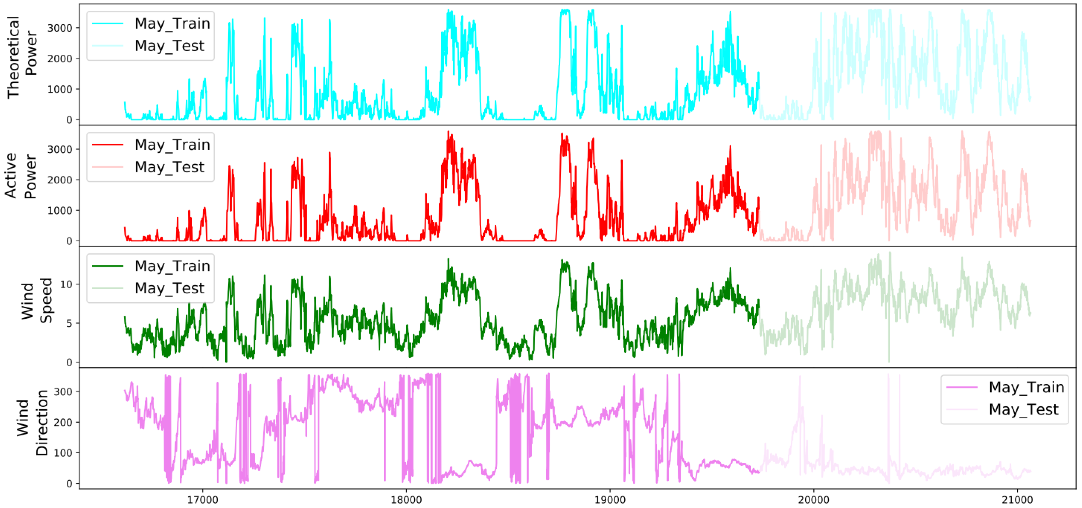
4.1. Train and Test Split

The dataset is not grouped in any way rather than by its four features to present the measurements for entire year. To do the forecasting for short term (i.e., every month), a filtering process is defined to count the number of elements for each month. At the same time, every month data is split into train and test sets by using a ratio of $70\%$ and $30\%$ respectively. The following Figure 13 presents one month data with train and test split for all four features collected by SCADA system.

4.2. Performance Measures

The three standard metrics the mean absolute error (MAE), mean squared error (MSE), and coefficient of determination ($R^2$) are used to measure the model prediction performance [26]. These measures are defined as follows:

$$\mathrm{MAE}(y,\widehat{y})=\frac{1}{n}\sum _{i=0}^{n-1}\left|y_i-{\widehat{y}}_i\right|$$

(16)

$$\mathrm{MSE}(y,\widehat{y})=\frac{1}{n}\sum _{i=0}^{n-1}{\left(y_i-{\widehat{y}}_i\right)}^2$$

(17)

$$R^2\left(y,\widehat{y}\right)=1-\frac{{\sum }_{i=0}^n{\left(y_i-{\widehat{y}}_i\right)}^2}{{\sum }_{i=0}^n\left(y_i-\overline{y}\right)}$$

(18)

In performance measures, y represents the observed value, $\widehat{y}$ is the predicted value, and n is total number of samples. In case of MAE and MSE the lower value of prediction correspond to high accuracy and $R^2$ value range between 0 and 1 and higher value corresponds to high performance.

4.3. Wind and Power Prediction

The obtained results are presented for active power, wind speed, its direction, and theoretical power for each month. Furthermore, the performance measures are presented for three months prediction. We also present the difference between actual and predicted value for understanding the actual error of the model.

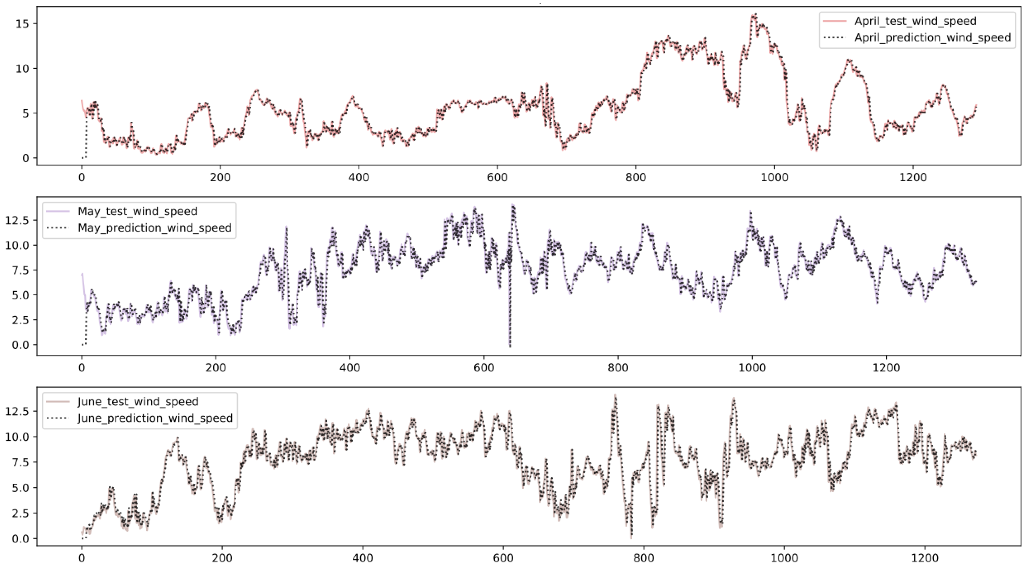
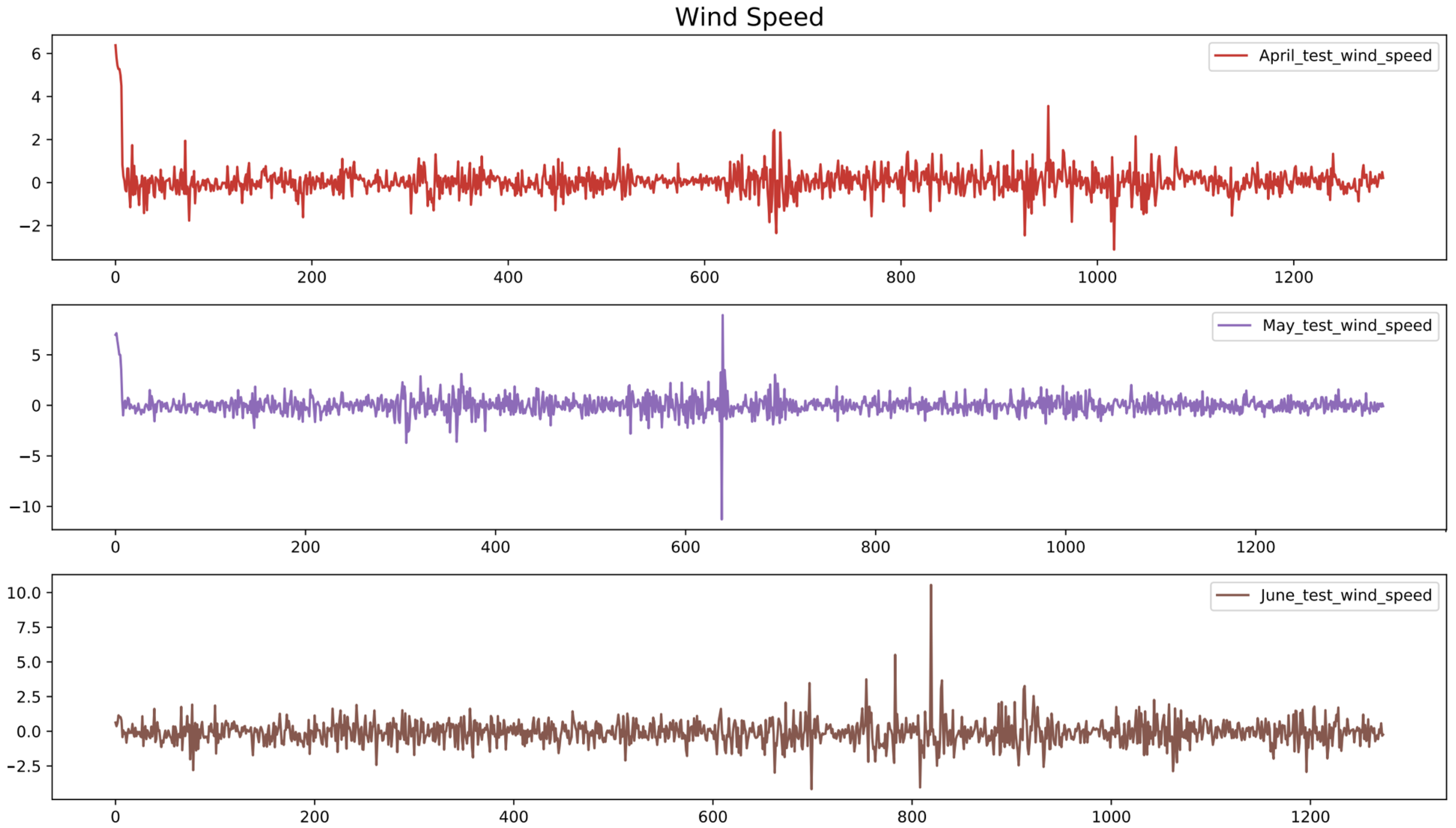
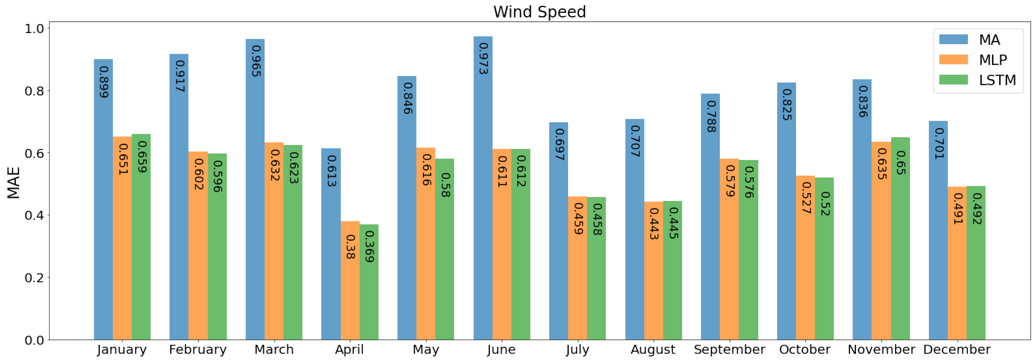
4.3.1. Wind Speed Prediction

The performance measures for wind speed prediction is presented in

Table 2. The performance measures of wind speed prediction over the test set for whole year.

Month	MAE	MSE	${\mathbf{R}}^2$
January	0.027	0.002	0.939
February	0.024	0.001	0.949
March	0.025	0.001	0.959
April	0.015	0.000	0.977
May	0.023	0.001	0.902
June	0.024	0.001	0.91
July	0.018	0.001	0.912
August	0.017	0.001	0.970
September	0.023	0.001	0.958
October	0.021	0.001	0.965
November	0.025	0.001	0.973
December	0.020	0.001	0.978

for the whole year. While, Figure 14 presents the predictions for the months of April, May, and June.

In Figure 14 the prediction seems that the predicted values are close to the actual values of wind speed. In order to know the subtle difference, the error graph is presented in Figure 15.

Figure 15 shows the consistent results as compared to the actual value of wind speed and few abrupt changes.

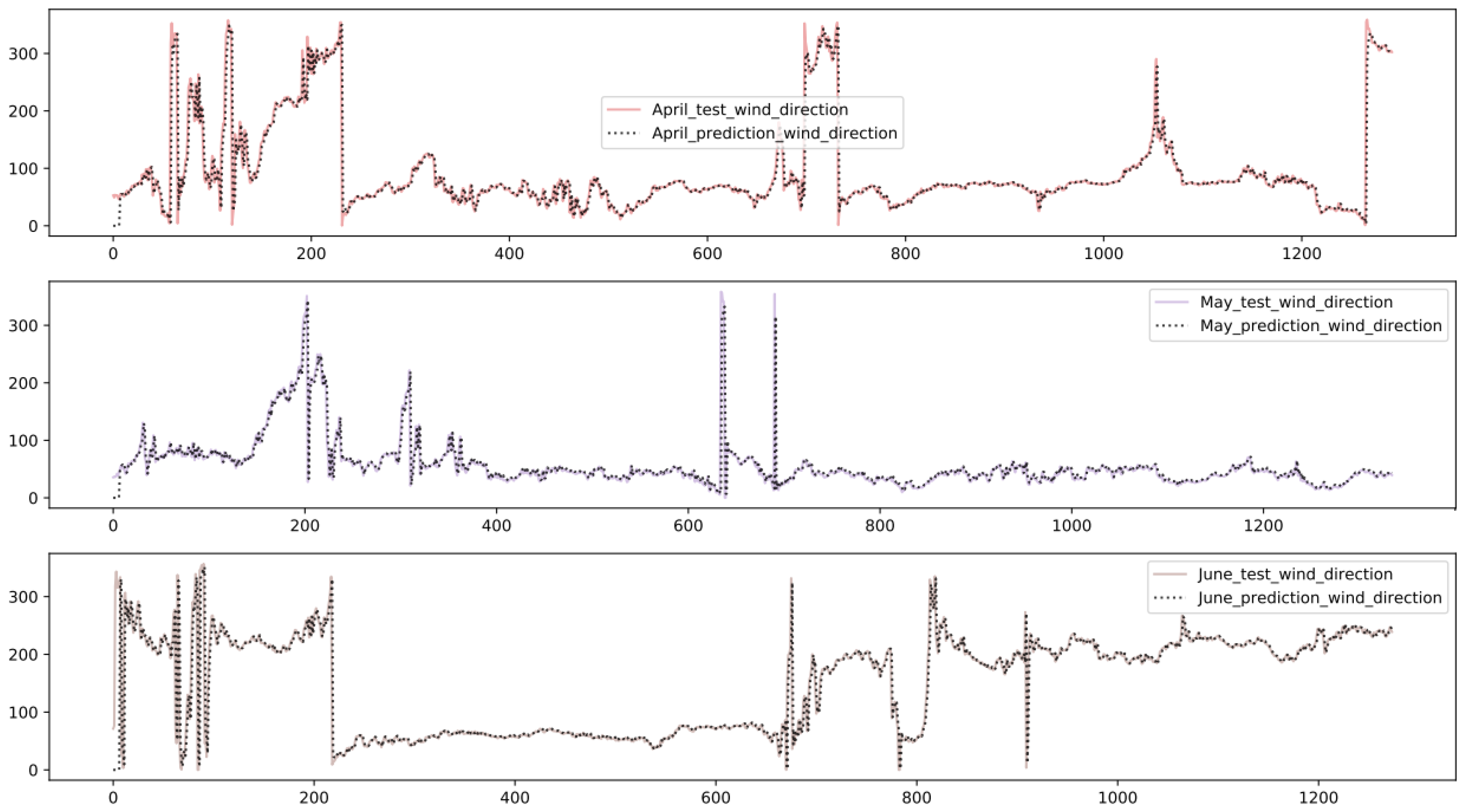
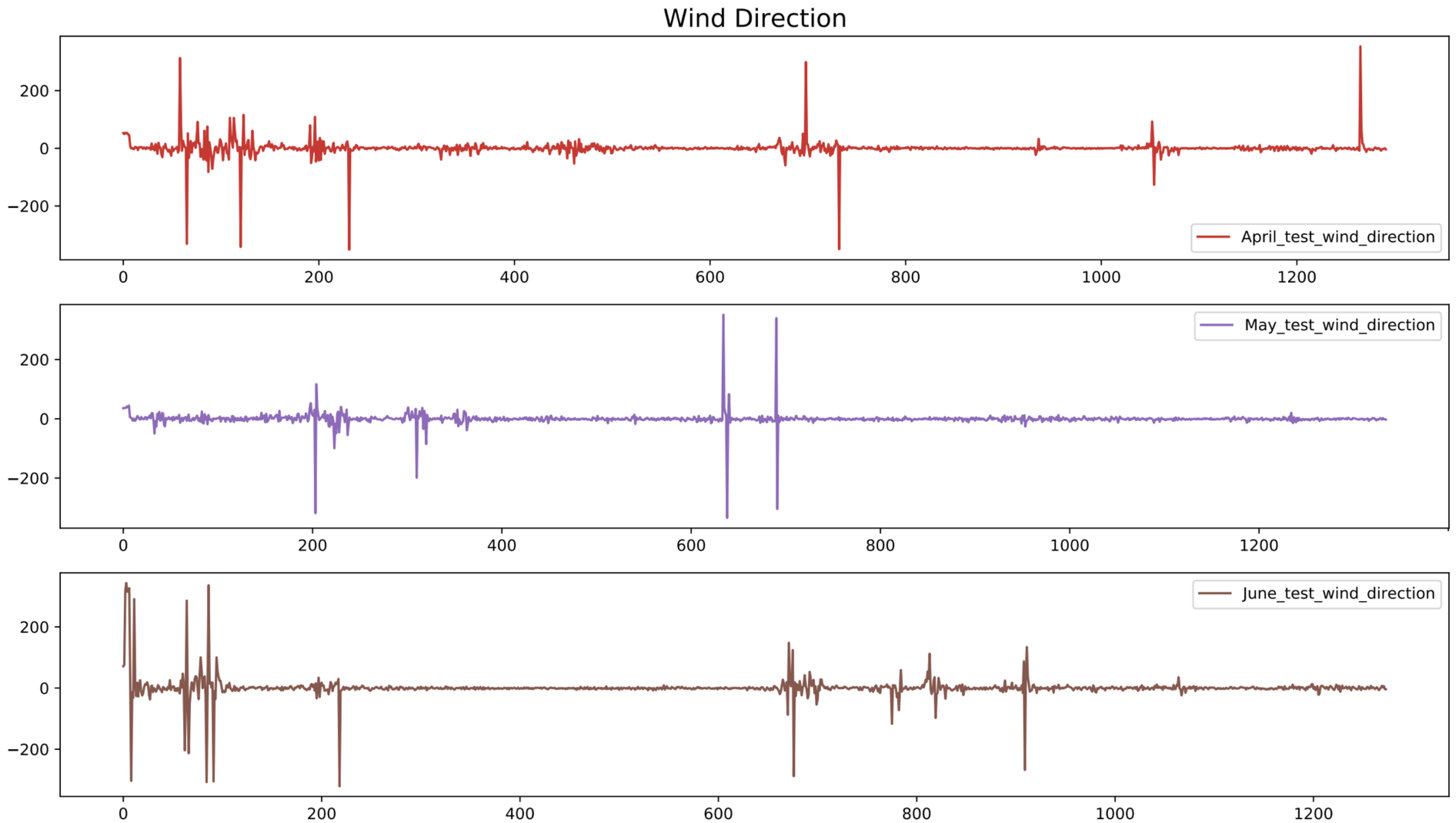
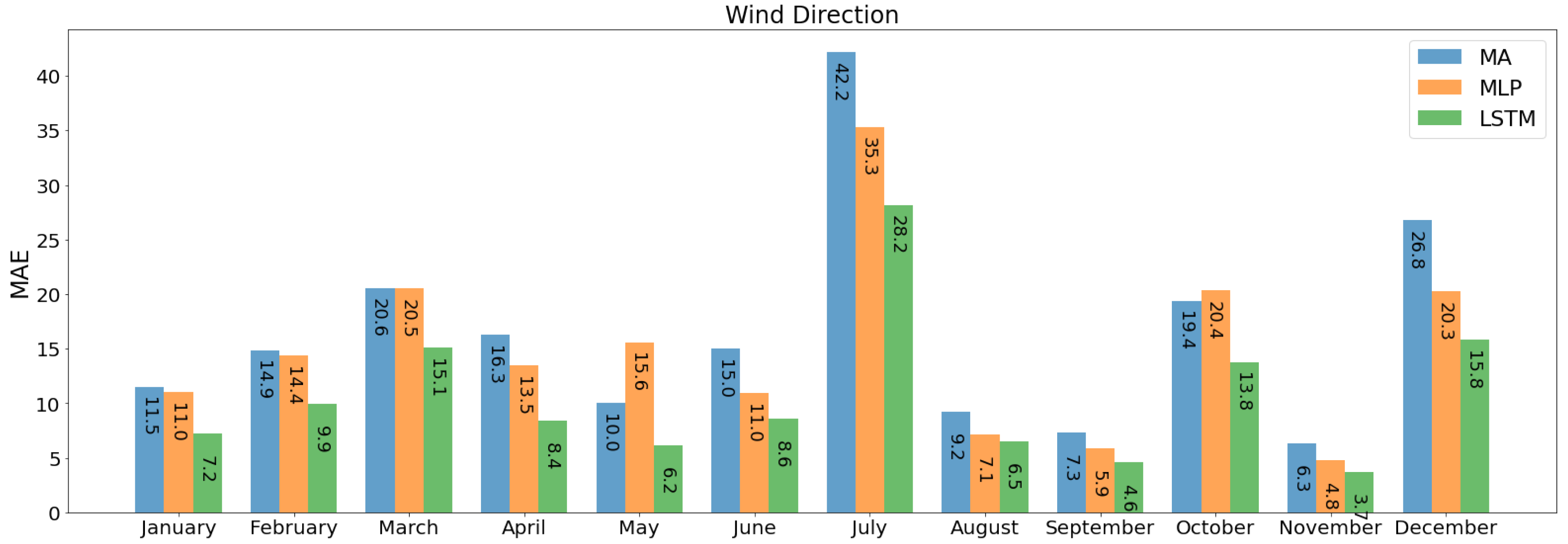
4.3.2. Wind Direction Prediction

The whole year wind direction prediction results are shown in

Table 3. The performance measures of wind direction prediction over the test set for whole year.

Month	MAE	MSE	${\mathbf{R}}^2$
January	0.03	0.008	0.888
February	0.028	0.01	0.785
March	0.042	0.024	0.57
April	0.025	0.006	0.866
May	0.017	0.004	0.733
June	0.023	0.006	0.877
July	0.079	0.047	0.556
August	0.018	0.007	0.365
September	0.013	0.001	0.954
October	0.038	0.024	0.366
November	0.011	0.001	0.975
December	0.045	0.025	0.738

and obtained results are accurate. Furthermore, Figure 16 and Figure 17 presents the predictions and obtained error for the months of April, May, and June.

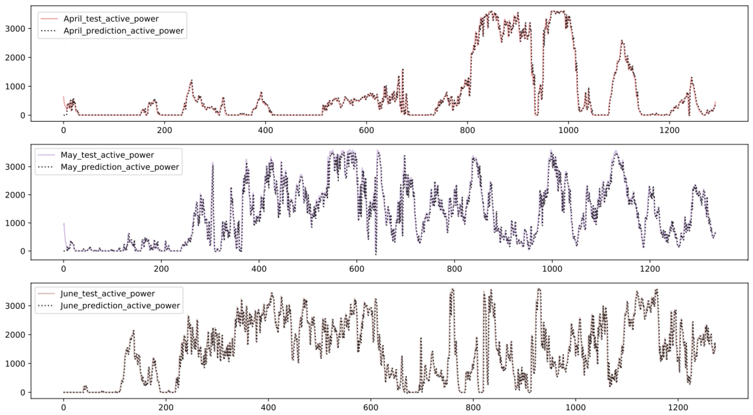
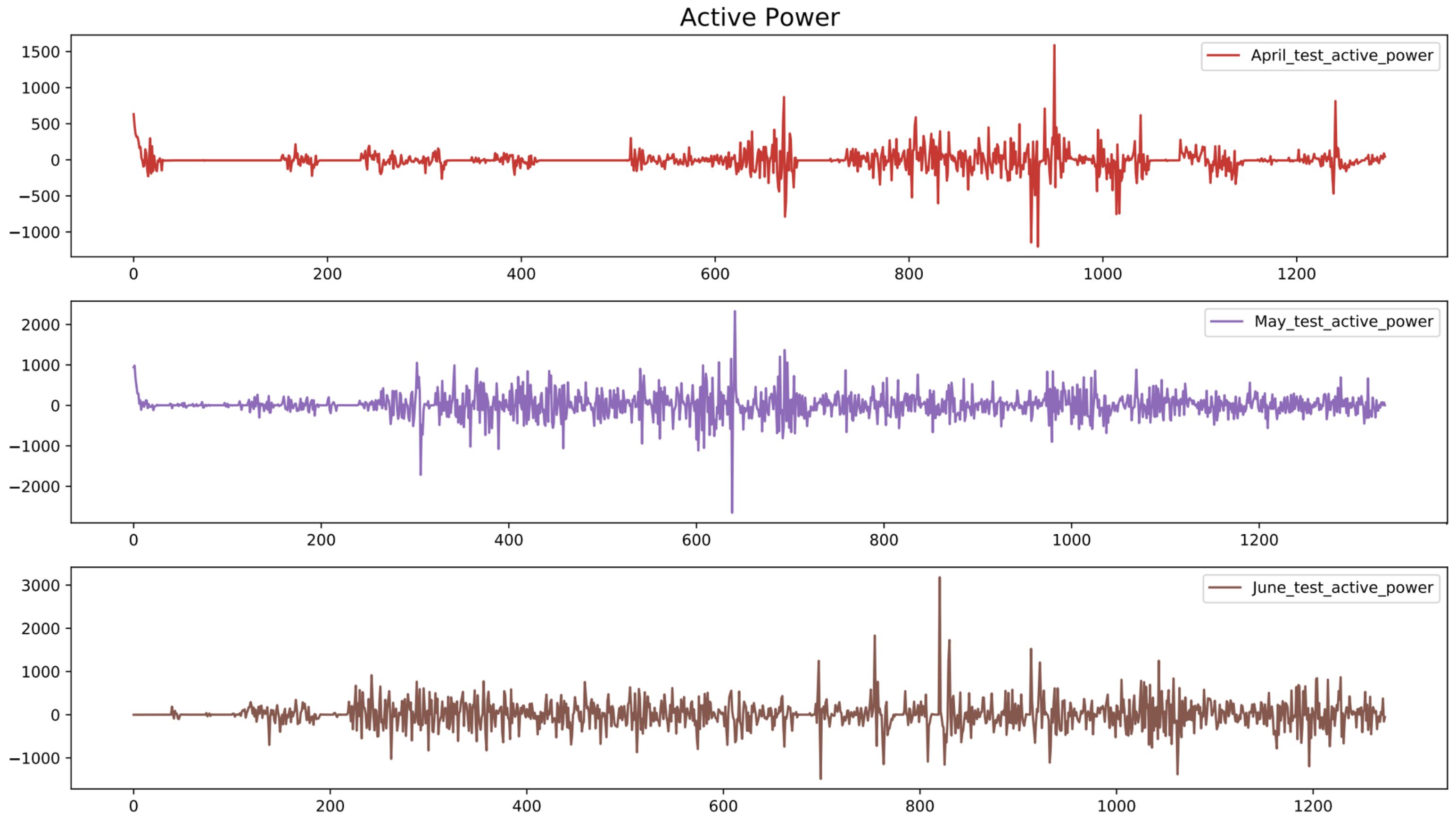
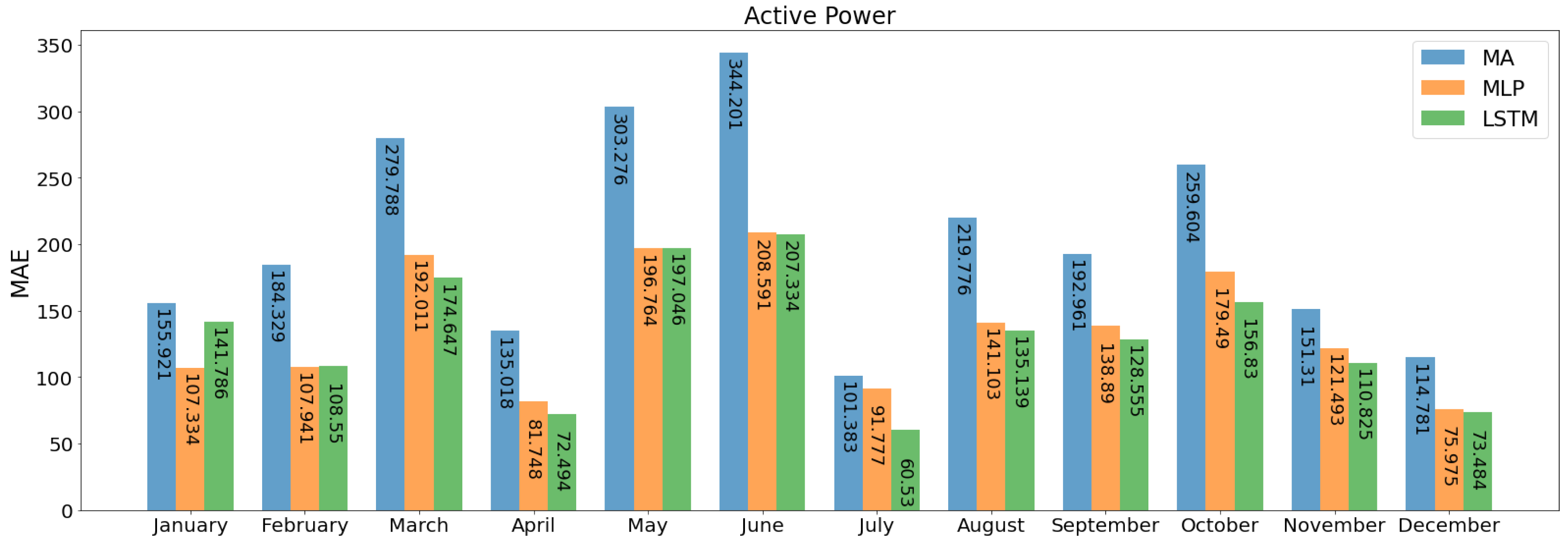
4.3.3. Active Power Prediction

The active power prediction results are shown in

Table 4. The performance measures of active power prediction over the test set for the whole year.

Month	MAE	MSE	${\mathbf{R}}^2$
January	0.031	0.006	0.966
February	0.028	0.004	0.955
March	0.049	0.008	0.945
April	0.019	0.001	0.983
May	0.054	0.007	0.917
June	0.057	0.008	0.906
July	0.016	0.002	0.912
August	0.037	0.003	0.97
September	0.036	0.003	0.976
October	0.044	0.005	0.961
November	0.029	0.004	0.975
December	0.02	0.003	0.98

and obtained results are accurate. Furthermore, Figure 18 present the predictions and Figure 19 presents the obtained error for the months of April, May, and June.

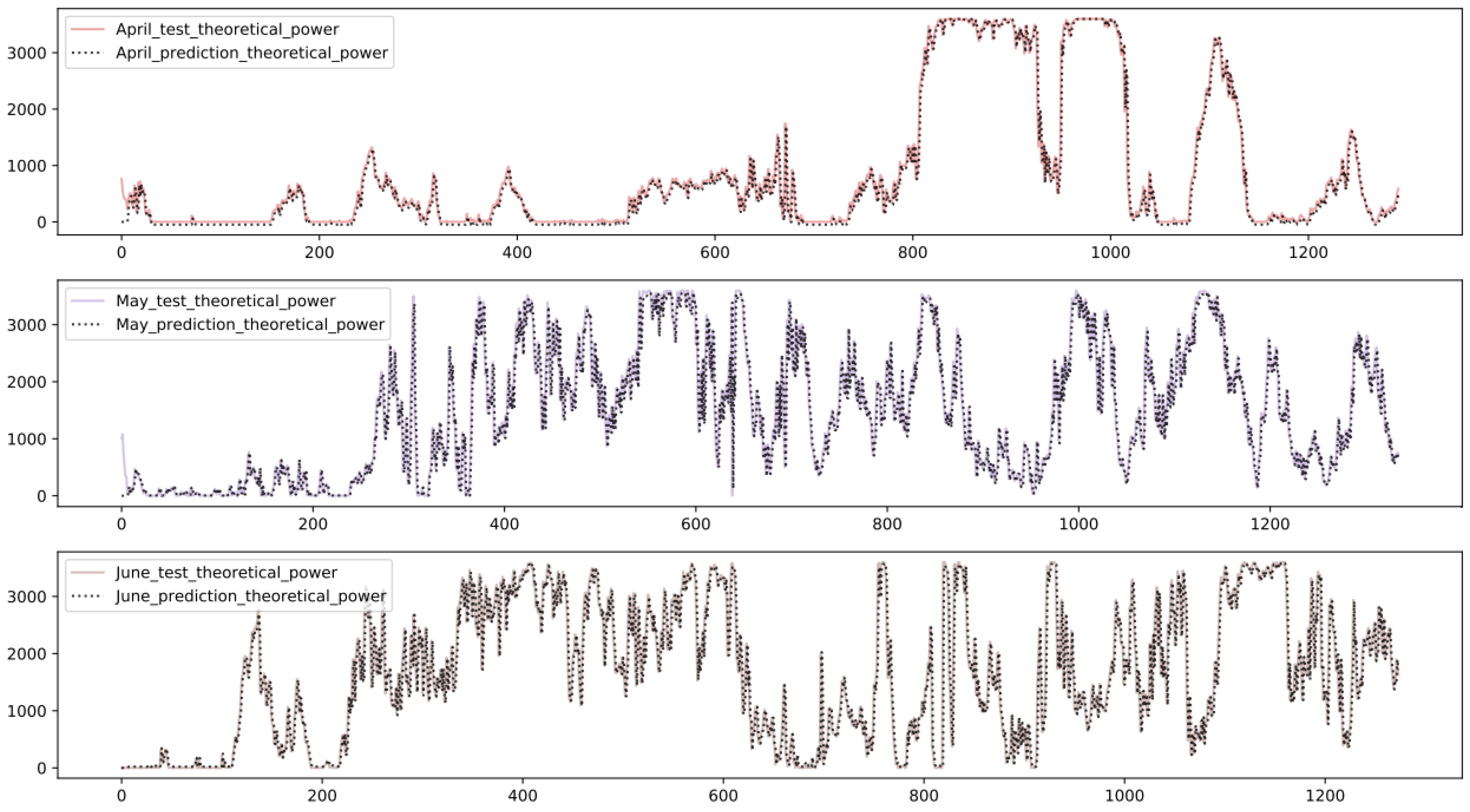
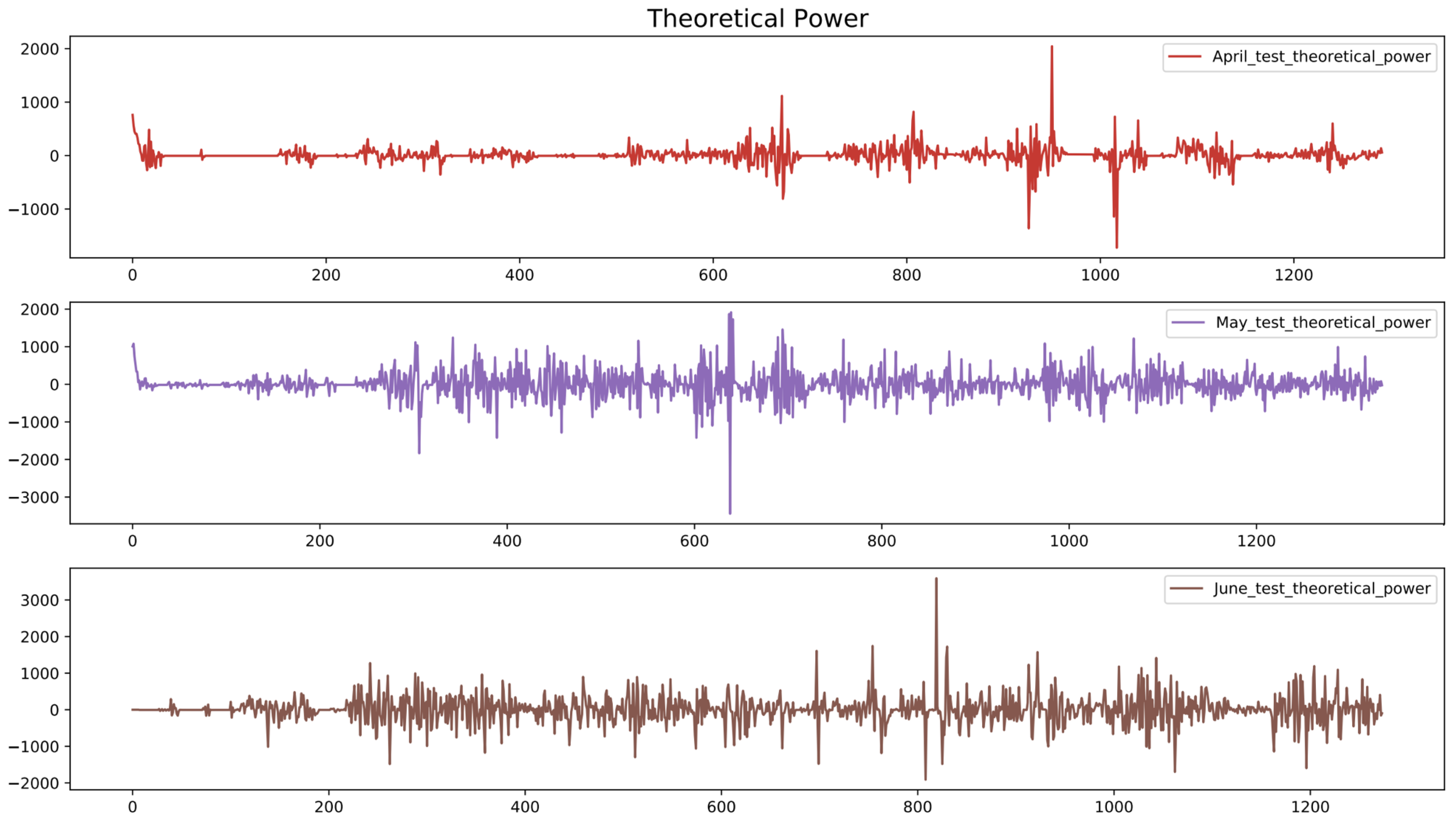
4.3.4. Theoretical Power Prediction

The theoretical power prediction results are shown in

Table 5. The performance measures of theoretical power prediction over the test set for the whole year.

Month	MAE	MSE	${\mathbf{R}}^2$
January	0.078	0.014	0.882
February	0.056	0.008	0.924
March	0.05	0.007	0.951
April	0.023	0.002	0.981
May	0.065	0.01	0.899
June	0.069	0.011	0.894
July	0.022	0.002	0.906
August	0.043	0.005	0.963
September	0.042	0.005	0.967
October	0.051	0.007	0.949
November	0.036	0.005	0.966
December	0.042	0.006	0.958

, Figure 20 present the predictions and Figure 21 presents the obtained error for the months of April, May, and June.

4.4. Comparative Analysis

A comparative analysis is performed to evaluate the performance between the proposed model and existing statistical and machine learning techniques. The comparison is made taking into account the statistical moving average technique (MA) and a multilayer perceptron (MLP) model. The metric used in this comparative analysis is mean absolute error (MAE). The lower value of MAE is better. The performance of each model is presented in the following subsections.

4.4.1. Active Power Prediction Comparison

The our model (i.e, LSTM) made least error scores for majority of the months between them all in nine out of twelve cases as it can be seen in Figure 22. The MLP got the least error score just in three cases and the MA in none of them.

In Figure 22, it is obvious to see that the results obtained from our proposed technique are consistent in all months and excluding the marginal cases.

4.4.2. Wind Speed Prediction Comparison

When predicting the wind speed our model (i.e., LSTM) got the least error scores in eight out of twelve cases as it can be seen in Figure 23. The MLP got the least error scores in four out of twelve cases, and the MA in none of them.

4.4.3. Wind Direction Prediction Comparison

When predicting the wind direction the LSTM got the least error score in twelve out of twelve cases as it is shown in Figure 24 outmatching the other two methods completely.

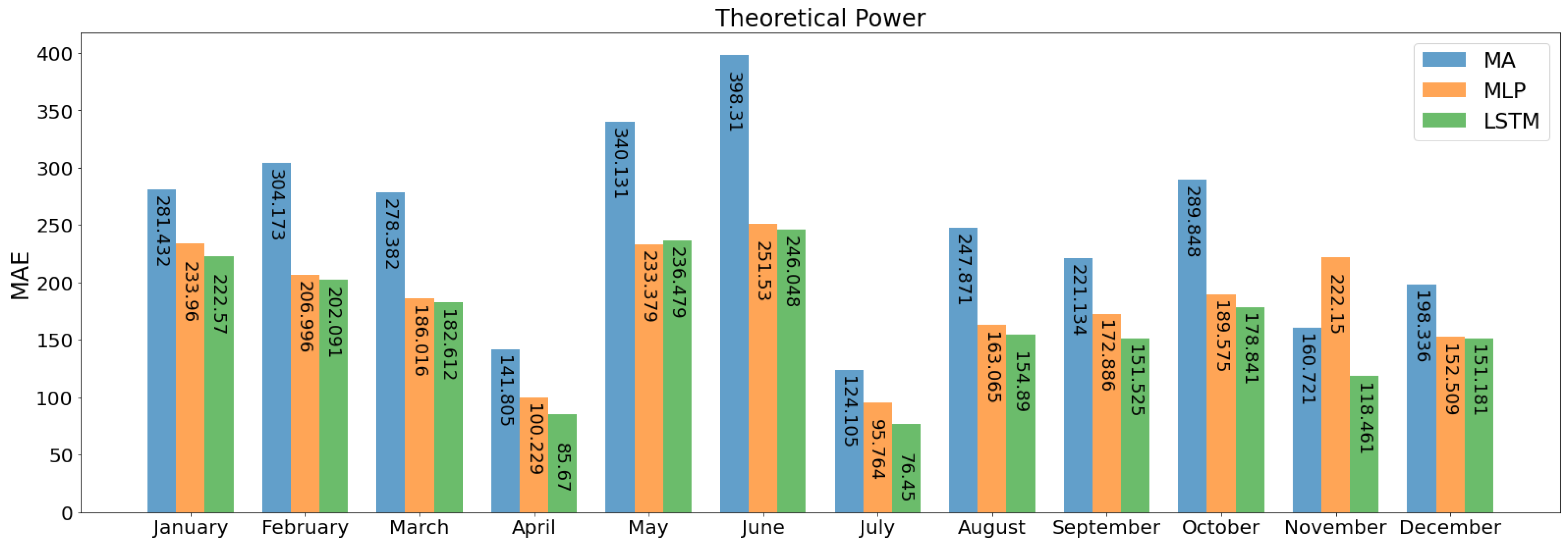
4.4.4. Theoretical Power Prediction Comparison

When predicting the theoretical power, the LSTM got the least error score in ten out of twelve as it is shown in Figure 25 while the MLP got the least error score in two out of twelve cases.

5. Conclusions

Wind turbines are one of the primary sources of clean and renewable energy. It can contribute to reduce global warming and save our planet. In this research, wind turbine data analysis and prediction are presented, which are based on SCADA system. The SCADA system generates time-series data continuously, which poses a challenge to analyze it in a timely manner. Our model can predict the short-term analysis for the wind and active power generation. The visualization-based data analysis can reduce the complexity of overall data logs to understand it. From the presented analysis, it can be concluded that wind speed and direction get stable at the start of a few days of every month. Wind direction determines the regions where the wind blows and its’ speed determines the amount of power to be produced. Furthermore, it may assist the wind farms management team to know the wind blowing patterns along with speed and active power generation. The developed LSTM-based prediction model provides short-term prediction about wind and power generation. It can effectively capture the dynamic behavior of wind energy. The comparison of the prediction results with the technique moving average (MA) and multilayer perceptron (MLP) technique shows that our model outperforms.

Our future work includes the multivariate time-series analysis by considering different factors for wind energy forecasting.

References

1. Mamat, R.; Sani, M.; Sudhakar, K. Renewable energy in Southeast Asia: Policies and recommendations. Sci. Total Environ. 2019, 670, 1095–1102. [Google Scholar]
2. Fahim, M.; Fraz, K.; Sillitti, A. TSI: Time Series to Imaging based Model for Detecting Anomalous Energy Consumption in Smart Buildings. Inf. Sci. 2020, 523, 1–13. [Google Scholar] [CrossRef]
3. Swart, R.; Robinson, J.; Cohen, S. Climate change and sustainable development: Expanding the options. Clim. Policy 2003, 3, S19–S40. [Google Scholar] [CrossRef]
4. Khosravi, A.; Machado, L.; Nunes, R. Time-series prediction of wind speed using machine learning algorithms: A case study Osorio wind farm, Brazil. Appl. Energy 2018, 224, 550–566. [Google Scholar] [CrossRef]
5. Ghiani, E.; Pisano, G. Impact of Renewable Energy Sources and Energy Storage Technologies on the Operation and Planning of Smart Distribution Networks. In Operation of Distributed Energy Resources in Smart Distribution Networks; Elsevier: Amsterdam, The Netherlands, 2018; pp. 25–48. [Google Scholar]
6. Zhang, Z.Y.; Wang, K.S. Wind turbine fault detection based on SCADA data analysis using ANN. Adv. Manuf. 2014, 2, 70–78. [Google Scholar] [CrossRef] [Green Version]
7. Gonzalez, E.; Stephen, B.; Infield, D.; Melero, J. On the use of high-frequency SCADA data for improved wind turbine performance monitoring. J. Phys. Conf. Ser. 2017, 926. [Google Scholar] [CrossRef]
8. Marti-Puig, P.; Blanco-M, A.; Cárdenas, J.J.; Cusidó, J.; Solé-Casals, J. Feature selection algorithms for wind turbine failure prediction. Energies 2019, 12, 453. [Google Scholar] [CrossRef] [Green Version]
9. Xiaodan, W.; Wenying, L.; Ningbo, W.; Yanhong, M. Short-term wind power prediction based on time series analysis model. In Proceedings of the 2nd International Conference on Computer Science and Electronics Engineering, Hangzhou, China, 22–23 March 2013. [Google Scholar]
10. Barbosa de Alencar, D.; de Mattos Affonso, C.; Limão de Oliveira, R.C.; Moya Rodriguez, J.L.; Leite, J.C.; Reston Filho, J.C. Different models for forecasting wind power generation: Case study. Energies 2017, 10, 1976. [Google Scholar] [CrossRef] [Green Version]
11. Pandit, R.K.; Infield, D. Performance Assessment of a Wind Turbine Using SCADA based Gaussian Process Model. Int. J. Prognostics Health Manag. 2018, 9, 64549. [Google Scholar]
12. Dai, J.; Yang, X.; Hu, W.; Wen, L.; Tan, Y. Effect investigation of yaw on wind turbine performance based on SCADA data. Energy 2018, 149, 684–696. [Google Scholar] [CrossRef]
13. Sun, H.; Gao, X.; Yang, H. A review of full-scale wind-field measurements of the wind-turbine wake effect and a measurement of the wake-interaction effect. Renew. Sustain. Energy Rev. 2020, 132, 110042. [Google Scholar] [CrossRef]
14. Gao, X.; Li, B.; Wang, T.; Sun, H.; Yang, H.; Li, Y.; Wang, Y.; Zhao, F. Investigation and validation of 3D wake model for horizontal-axis wind turbines based on filed measurements. Appl. Energy 2020, 260, 114272. [Google Scholar] [CrossRef]
15. Sun, H.; Qiu, C.; Lu, L.; Gao, X.; Chen, J.; Yang, H. Wind turbine power modelling and optimization using artificial neural network with wind field experimental data. Appl. Energy 2020, 280, 115880. [Google Scholar] [CrossRef]
16. Schmidhuber, J. Deep learning in neural networks: An overview. Neural Netw. 2015, 61, 85–117. [Google Scholar] [CrossRef] [PubMed] [Green Version]
17. Chen, K.; Zhou, Y.; Dai, F. A LSTM-based method for stock returns prediction: A case study of China stock market. In Proceedings of the 2015 IEEE International Conference on Big Data (Big Data), Santa Clara, CA, USA, 29 October–1 November 2015; pp. 2823–2824. [Google Scholar]
18. Wang, S.; Jiang, J. Learning Natural Language Inference with LSTM. arXiv 2016, arXiv:1512.08849. [Google Scholar]
19. Lipton, Z.C.; Kale, D.C.; Elkan, C.; Wetzel, R. Learning to Diagnose with LSTM Recurrent Neural Networks. arXiv 2016, arXiv:1511.03677. [Google Scholar]
20. Liu, Y.; Guan, L.; Hou, C.; Han, H.; Liu, Z.; Sun, Y.; Zheng, M. Wind power short-term prediction based on LSTM and discrete wavelet transform. Appl. Sci. 2019, 9, 1108. [Google Scholar] [CrossRef] [Green Version]
21. Son, N.; Yang, S.; Na, J. Hybrid Forecasting Model for Short-Term Wind Power Prediction Using Modified Long Short-Term Memory. Energies 2019, 12, 3901. [Google Scholar] [CrossRef] [Green Version]
22. Erisen, B. Wind Turbine Scada Dataset. 2018. Available online: https://www.kaggle.com/berkerisen/wind-turbine-scada-dataset (accessed on 23 December 2020).
23. Bergey, K.H. The Lanchester-Betz limit (energy conversion efficiency factor for windmills). J. Energy 1979, 3, 382–384. [Google Scholar] [CrossRef]
24. Hochreiter, S.; Schmidhuber, J. Long Short-Term Memroy. Neural Comput. 1997, 9, 1735–1780. Available online: https://www.bioinf.jku.at/publications/older/2604.pdf (accessed on 8 May 2012). [CrossRef] [PubMed]
25. Kong, W.; Dong, Z.Y.; Jia, Y.; Hill, D.J.; Xu, Y.; Zhang, Y. Short-term residential load forecasting based on LSTM recurrent neural network. IEEE Trans. Smart Grid 2017, 10, 841–851. [Google Scholar] [CrossRef]
26. Ghofrani, M.; Suherli, A. Time series and renewable energy forecasting. Time Ser. Anal. Appl. 2017, 2017, 77–92. [Google Scholar]
Figure 1. The proposed model of wind turbine data analysis and prediction.
Energies 14 00125 g001
Figure 2. One week data representation of wind turbine gathered by supervisory control and data acquisition (SCADA) system.
Energies 14 00125 g002
Figure 3. The one month data visualization in cylindrical coordinates with possible analysis.
Energies 14 00125 g003
Figure 4. Scatter plot for the whole year with wind direction, wind speed, and active power.
Energies 14 00125 g004
Figure 5. Scatter plot for the months of July, September and October individually along with Wind Direction, Wind Speed, and Active Power.
Energies 14 00125 g005
Figure 6. Wind turbine Scada dataset 2D visualization in polar coordinates.
Energies 14 00125 g006
Figure 7. The wind speed and direction for the month of April, May, and June.
Energies 14 00125 g007
Figure 8. Wind turbine Scada dataset 3D visualization in cylindrical coordinates.
Energies 14 00125 g008
Figure 9. Wind Speed vs. Wind Direction vs. Active Power.
Energies 14 00125 g009
Figure 10. The wind speed with direction and time as a vertical axis to observe the blowing pattern.
Energies 14 00125 g010
Figure 11. Wind energy generation in terms of active power, and theoretical power.
Energies 14 00125 g011
Figure 12. A long short term memory (LSTM) cell representation.
Energies 14 00125 g012
Figure 13. The theoratical power, active power, wind speed, and wind direction for one month of train, and test.
Energies 14 00125 g013
Figure 14. The wind speed predictions for the test set of April, May, and June.
Energies 14 00125 g014
Figure 15. The difference between the actual and predicted value of wind speed over the test set of April, May, and June.
Energies 14 00125 g015
Figure 16. The wind direction predictions for the test set of April, May, and June.
Energies 14 00125 g016
Figure 17. The difference between the actual and predicted value of wind direction over the test set of April, May, and June.
Energies 14 00125 g017
Figure 18. The active power predictions for the test set of April, May, and June.
Energies 14 00125 g018
Figure 19. The difference between the actual and predicted value of active power generation over the test set of April, May, and June.
Energies 14 00125 g019
Figure 20. The theoretical power predictions for the test set of April, May, and June.
Energies 14 00125 g020
Figure 21. The difference between the actual and predicted value of theoretical power over the test set of April, May, and June.
Energies 14 00125 g021
Figure 22. The performance metric (MAE) comparison for active power prediction for the whole year.
Energies 14 00125 g022
Figure 23. The performance metric (MAE) comparison for wind speed prediction for the whole year.
Energies 14 00125 g023
Figure 24. The performance metric (MAE) comparison for wind direction prediction for the whole year.
Energies 14 00125 g024
Figure 25. The performance metric (MAE) comparison for theoretical power prediction for whole year.
Energies 14 00125 g025