Building Suitable Datasets for Soft Computing and Machine Learning Techniques from Meteorological Data Integration: A Case Study for Predicting Significant Wave Height and Energy Flux

 , , ,
, , ,  and
and
Abstract
1. Introduction
- The generation of datasets becomes a very easy and customisable task by means of the selection of different input parameters, such as predictive and objective variables, classification and regression, output discretisation (useful for ordinal regression) or prediction horizon, among others.
- The created datasets can be easily used by SC and ML tools.
- It makes the researcher focus on environmental modelling, without having to worry about the development of scripts or mechanical tasks, avoiding laborious pre-processing procedures that imply a great deal of time and endeavour in early stages of the research.
- It avoids possible researcher errors in the intermediate steps of the process, such as geographical coordinates conversion, missing values handling (dates or measurements not recorded) or different temporal resolution of the data collected, among others.
- It provides information about the quality and quantity of the data. SPAMDA allows preliminary studies of missing values (dates or measurements not recorded) in buoys managed by NDBC, so that the researcher can have an idea of the quality of the data recorded by the buoys and about their suitability for the intended purpose. In any case, SPAMDA allows data integration taking into account such missing values when needed by the user.
- Estimation of the amount of energy flux that can be produced at different prediction horizons: short-term, mid-term or long-term. Although this work does not focus on model performance, it should be taken into account that models tend to generalise worse with greater prediction horizons.
- It manages the extensive casuistry of data integration which can lead to incomplete datasets, described in Appendix A.
- Possibility of selecting one or more reanalysis nodes near the localisation under study, which could provide a better description of the problem to achieve more accurate models.
- Although pre-processing is not the main objective of SPAMDA, the tool also provides some basic pre-processing filters on buoy measurements, such as normalisation and missing data recovery.
- It facilitates data management and well-organised storage of the datasets. Environmental studies in different geographical locations can be carried out by merely introducing and using other collected data.
- SPAMDA is distributed as an open source tool, its modular design allows the implementation of new modules for managing meteorological data from other sources, benefiting future renewable energy and environmental research.
- It includes a user-friendly GUI, facilitating and greatly simplifying data management, and it is integrated with the Explorer environment of WEKA.
- It is multi-platform, and it can be used on any computer with Java regardless of the operating system.
2. Meteorological Data Sources
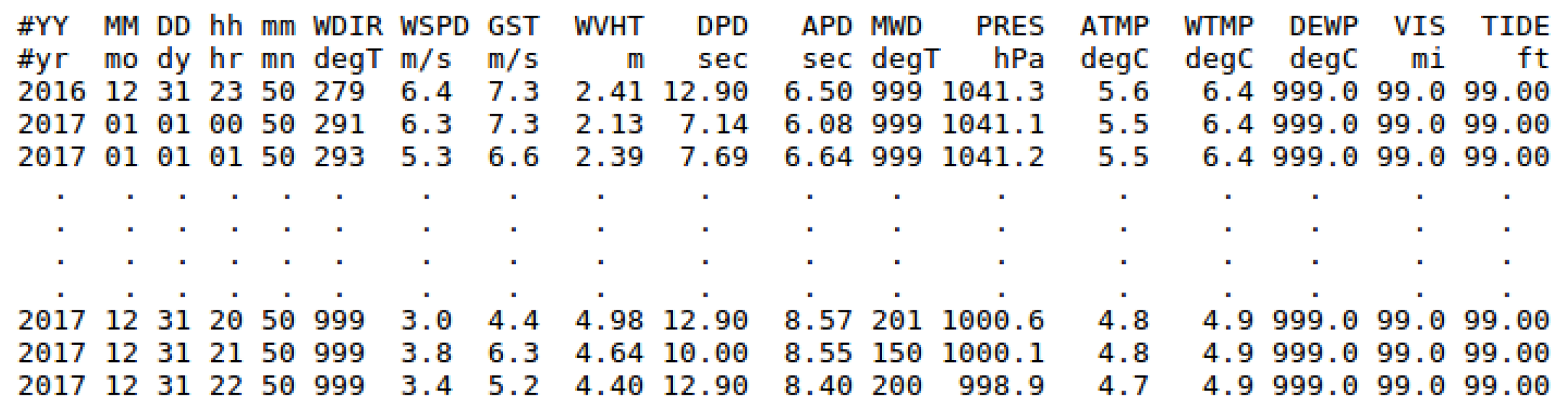
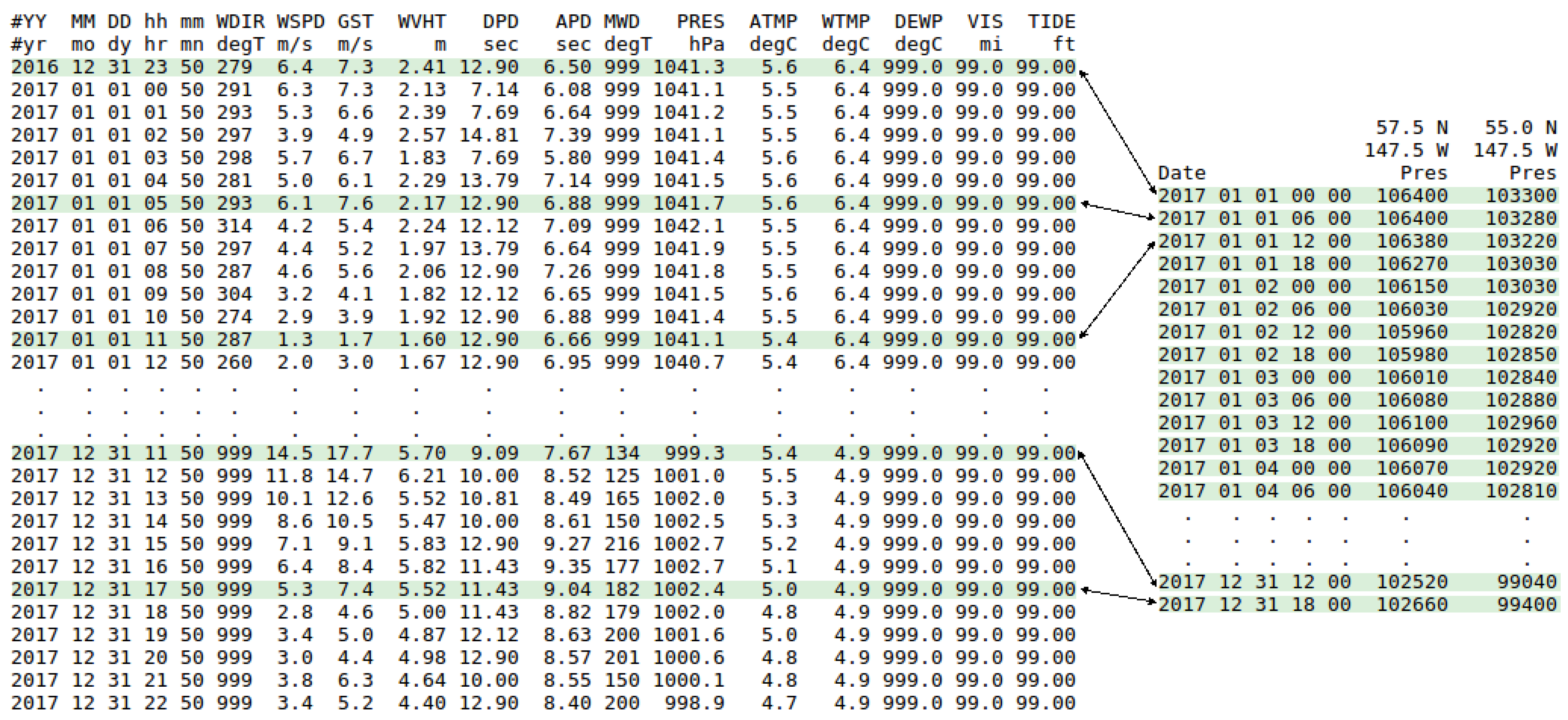
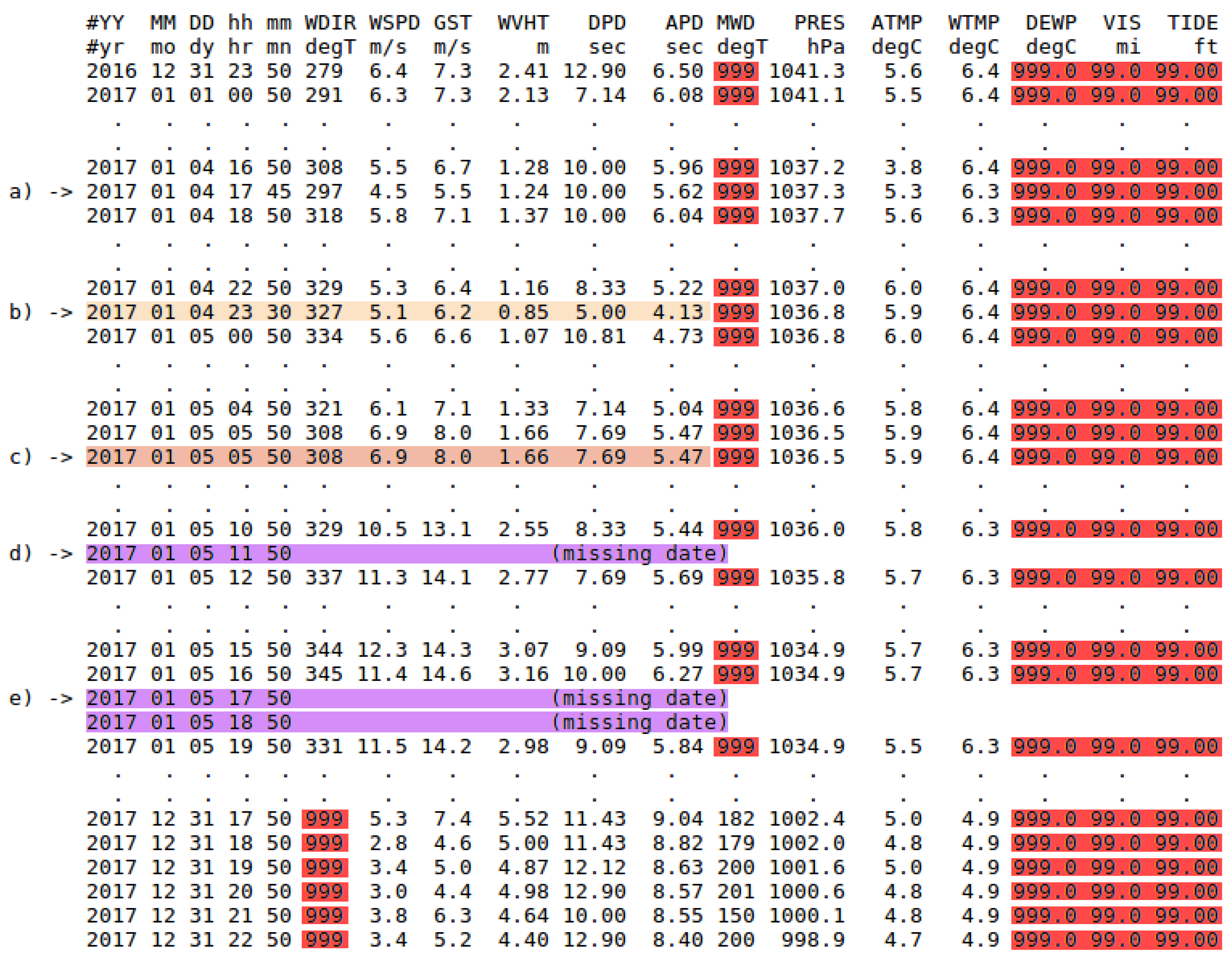
- NDBC belongs to the National Weather Service (NWS) and operates and supports a network of marine and ocean buoys that record data. The mission of the network is to record marine and ocean meteorological data, such as , dominant wave period, or wind speed and direction, among others.The buoys maintained by NDBC are located in coastal and offshore waters, and they are provided with specific sensors and devices which allow them to perform measurements. The information collected by the buoys is available on the NDBC website [58], and it is divided into different groups. One of them corresponds to standard meteorological information of the historical data collected by each buoy, which can be downloaded as annual text files and whose format was adopted by NDBC since January 2007 [59]. These files contain hourly measurements per day from 00:50 to 23:50 UTC (Universal Time Coordinated) and from 23:50 31 December of the previous desired year to 22:50 31 December of the desired year. In Table 1, a comprehensive measurement description and the corresponding units are provided as a summary for the reader. A fragment of one of these files, which contains the measurements collected during year 2017 by the buoy identified as Station 46001 in NDBC, is shown in Figure 1. Each column corresponds to a meteorological variable or attribute, and each row or instance corresponds to the values of the measurements collected by the buoy for each attribute at a specific date and time.Note that the data collected by the network of buoys may be incomplete due to diverse circumstances such as the weather conditions in which the buoys have to operate, failures or malfunctioning elements of the buoys, among others. Accordingly, it may be the situation that some of the measurements are completely missing (missing date or instance) or partially missing (some measurements not recorded), by a buoy or by a set of buoys, once in a while or over a period of time. It may be also possible that the measurements have been recorded at a time different from the expected one. These aspects have to be taken into account when creating the datasets. This casuistry is explained in detail in Appendix A.
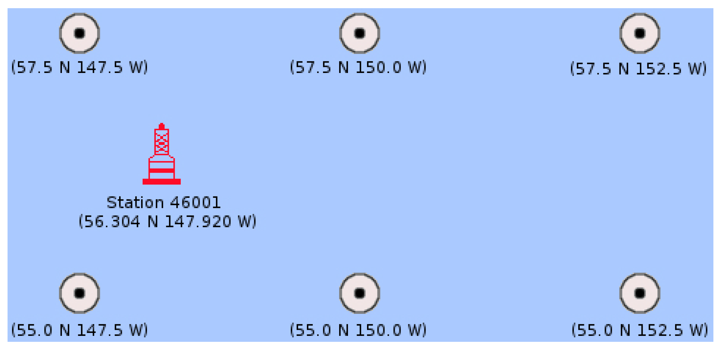
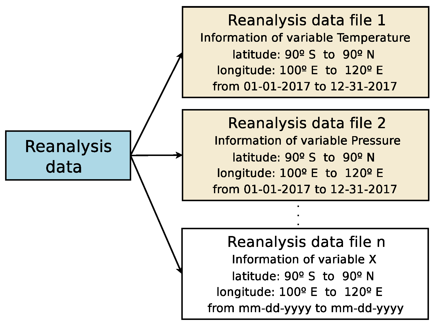
- NNRP provides three-dimensional global reanalysis of numerous meteorological observations (e.g., components Zonal and Meridional of the velocity of the wind, relative humidity, pressure, etc.), which is available monthly, daily, and every six hours at 00 Z (Zulu time), 06 Z, 12 Z, and 18 Z from 1948 on a global × grid. Weather observations are from different sources, such as ships, satellites, and radar, among others. Reanalysis data are created assimilating such observations employing the same climate model along the whole period of reanalysis in order to decrease the impact of modelling changes on climate statistics. Such information has become a substantial support of the needs of the research community, even more in locations where instrumental (real time) data are not available.The reanalysis data are available in the NNRP website [61], which is accessible through different sections. Such data can be fully (a global × grid) or partially (only the desired reanalysis nodes or sub-grid) downloaded as Network Common Data Form (NetCDF) files [62], a special binary format for representing scientific data, which provides a description of the file contents and also includes the spatial and temporal properties of the data. Each reanalysis file contains the values of a meteorological variable estimated by a mathematical model for each reanalysis node. For the sake of clarity, in Figure 2, an example to approximately illustrate a sub-grid containing six nodes of reanalysis surrounding the geographic localisation of a buoy (obtained from NDBC) is shown.Therefore, with both sources of information, which complement each other, and carrying out a matching process, SPAMDA will create datasets for prediction tasks. In this way, the dataset input variables will be one or more reanalysis variables from NNRP and one or more measurements from NDBC. The dataset output variable will always be one measurement from NDBC.
3. SPAMDA
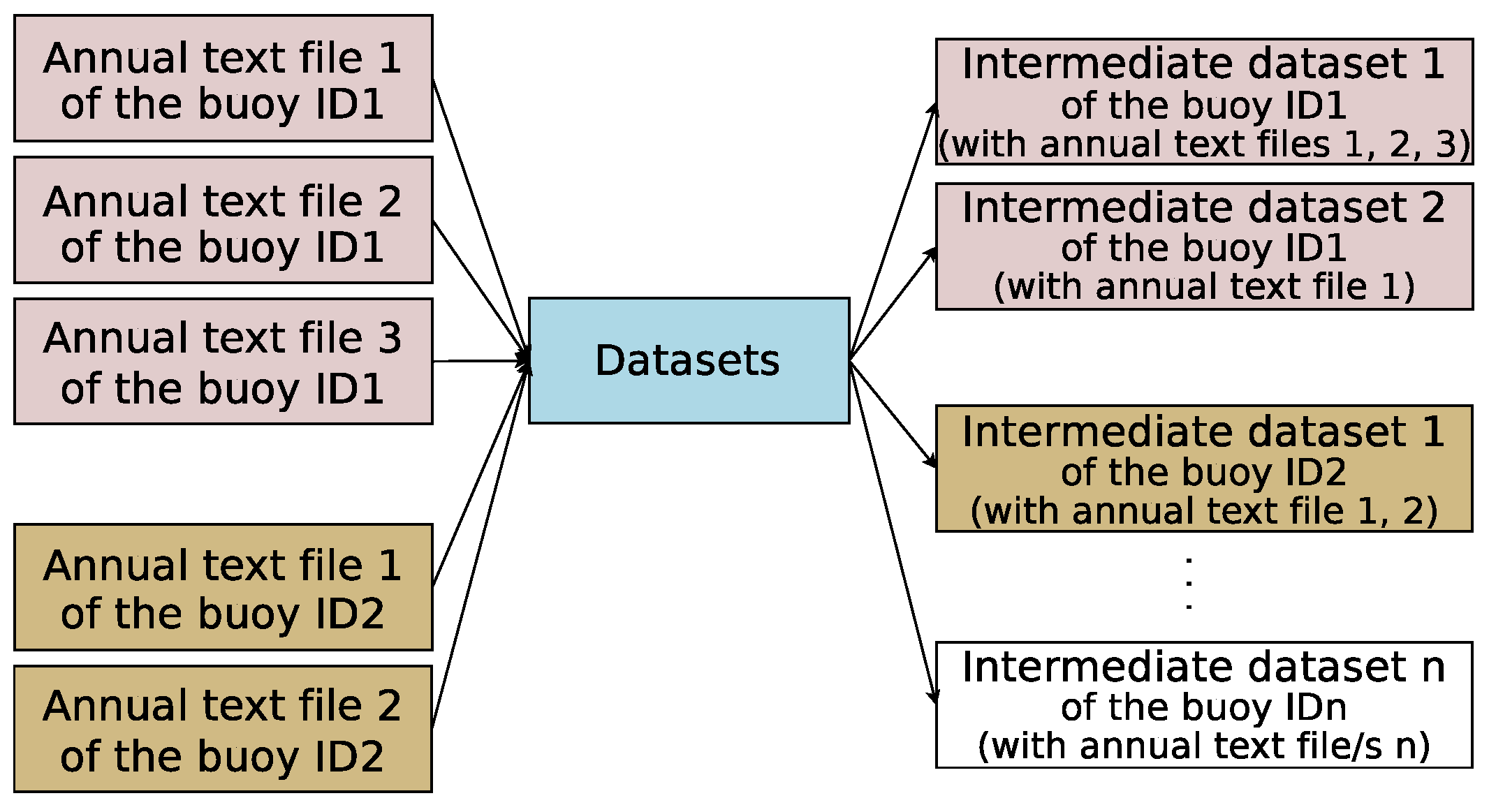
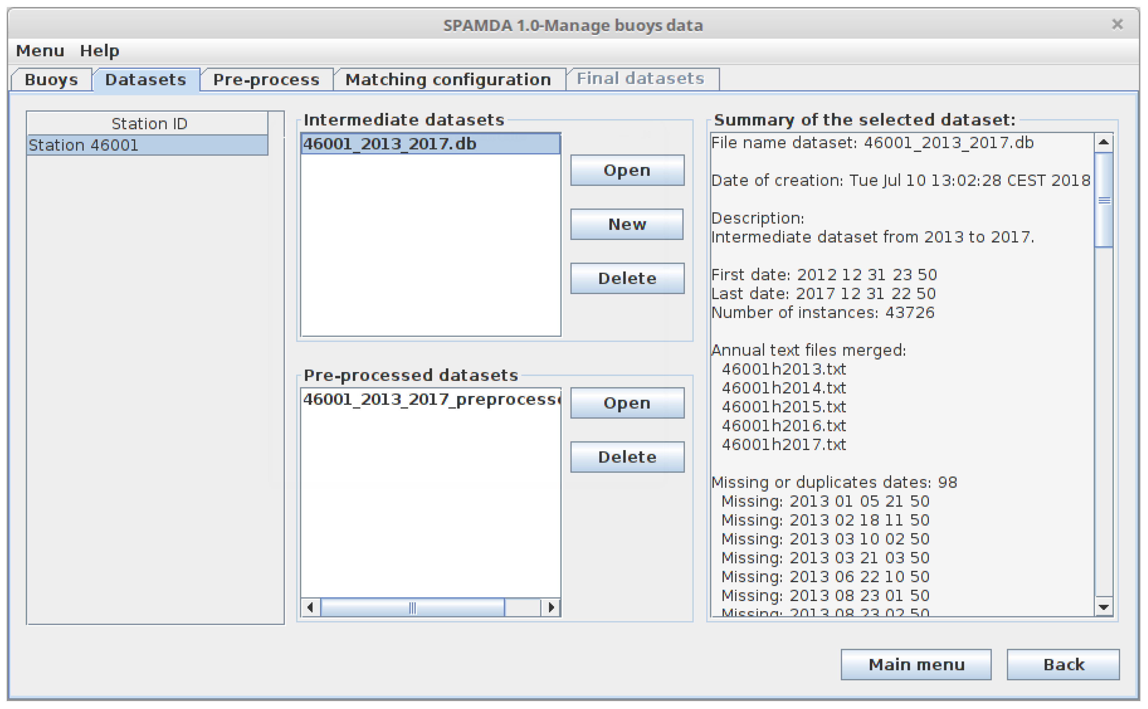
- Intermediate datasets: They contain the meteorological observations from NDBC.
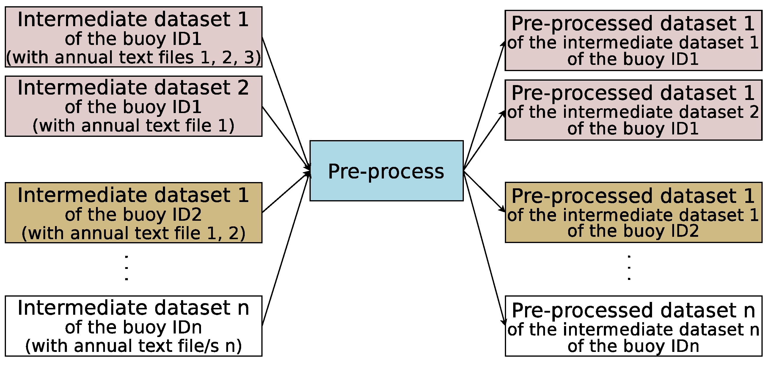
- Pre-processed datasets: They are obtained as a result of pre-processing tasks performed on the intermediate datasets.
- Final datasets: Created by merging an intermediate or pre-processed dataset (which contain the information from NDBC) with the reanalysis data from NNRP. This procedure is referenced in SPAMDA as a matching process and will be carried out according to the study to be performed (classification or regression).
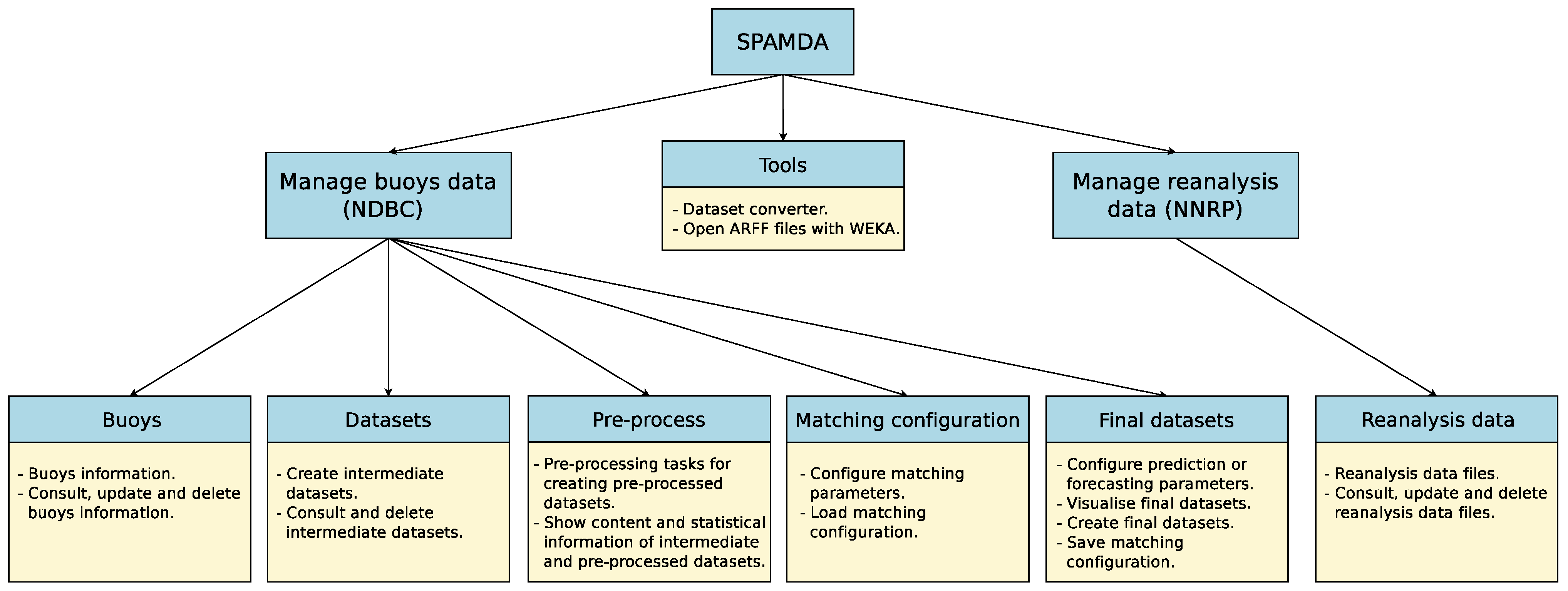
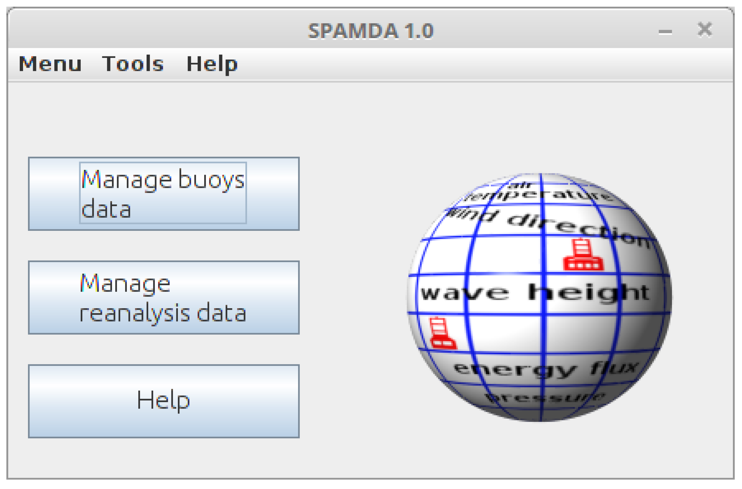
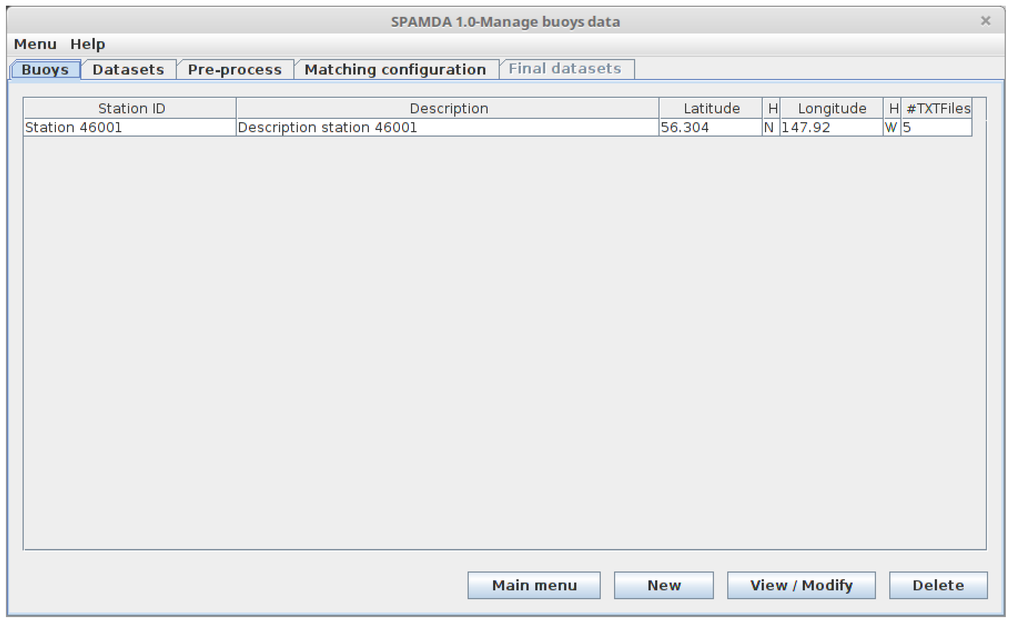
- Manage buoys data: The aim of this module is to provide features for the management and analysis of the information related to the buoys from NDBC. This includes:
- Entering and updating the information of each buoy.
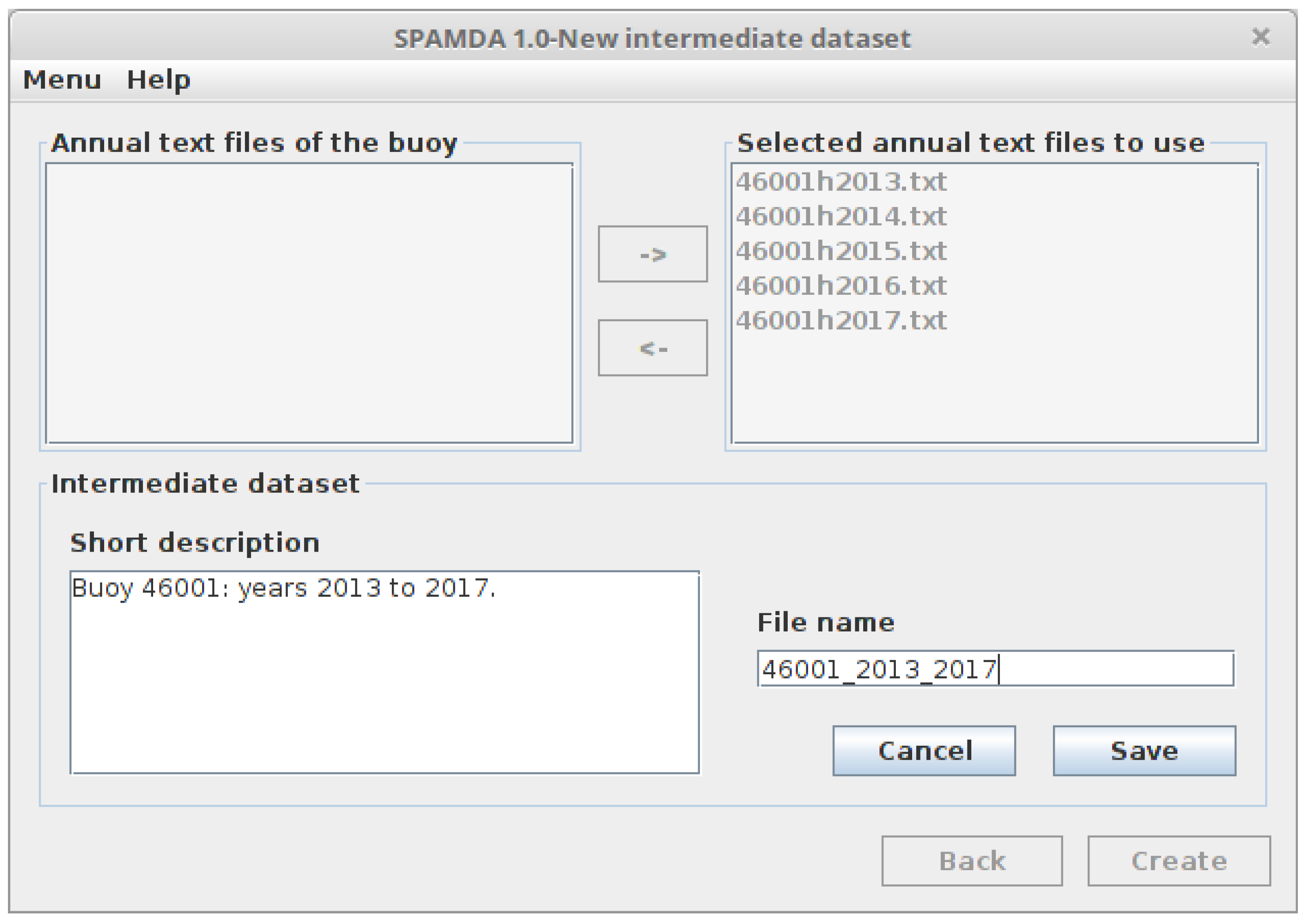
- Creation of intermediate datasets with the collected measurements.
- Pre-processing tasks for obtaining the pre-processed datasets.
- Matching process to merge the information from NDBC and NNRP.
- Creation of the final datasets according to the ML technique to use (classification or regression).
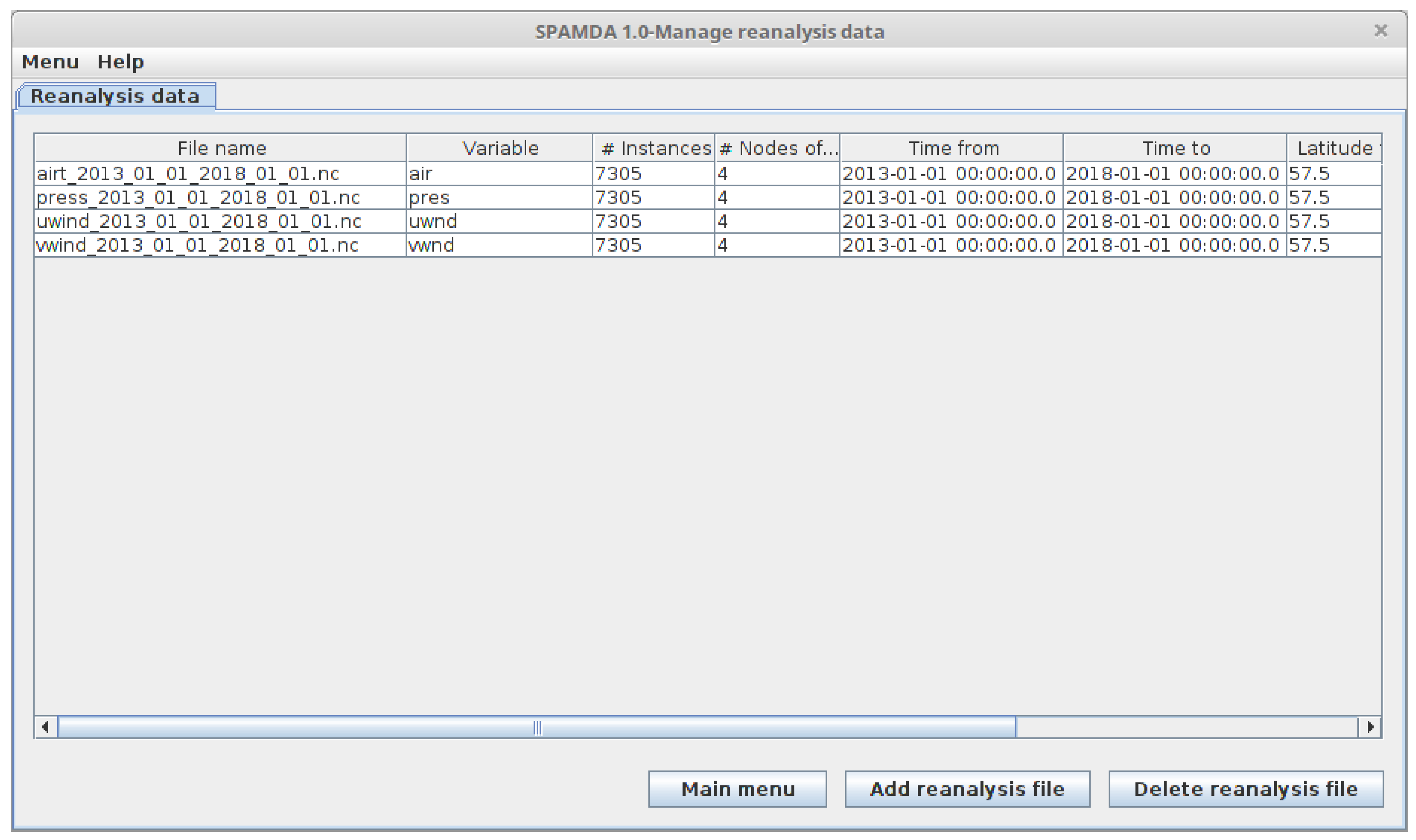
- Manage reanalysis data: This module is used for the management of the reanalysis data provided by the NNRP. In this way, researchers can keep the reanalysis data files updated for their studies. Such files will be used, depending on researchers’ needs, in the matching process when obtaining the final datasets.
- Tools: This module includes features for converting intermediate or pre-processed datasets to ARFF or CSV format and for opening ARFF files with WEKA software.
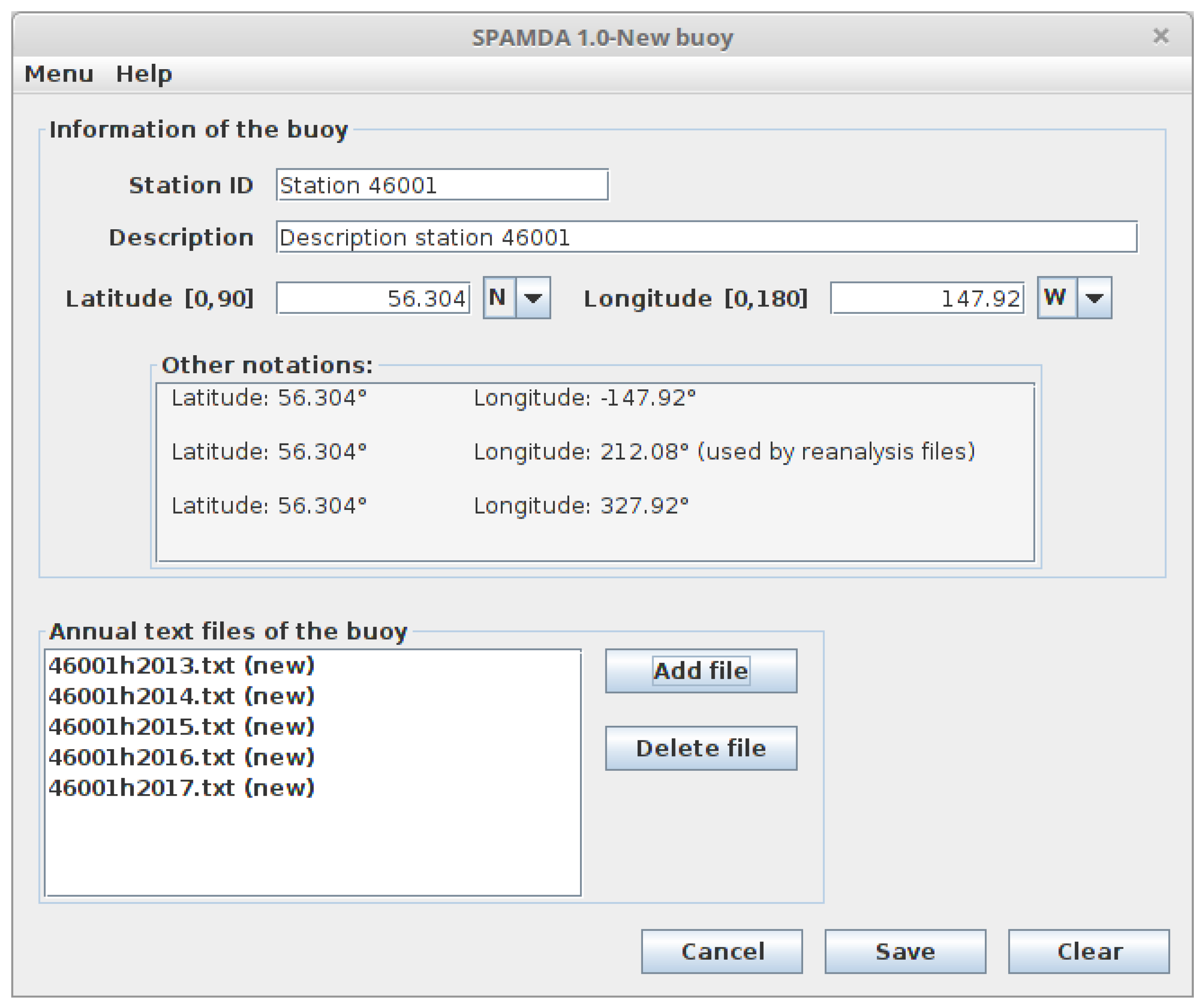
3.1. Buoys
- Station ID: An alphanumeric identifier that allows easy identification of the buoy.
- Description: A short description of the buoy.
- Latitude: North or South geographical localisation (degrees) of the buoy.
- Longitude: West or East geographical localisation (degrees) of the buoy.
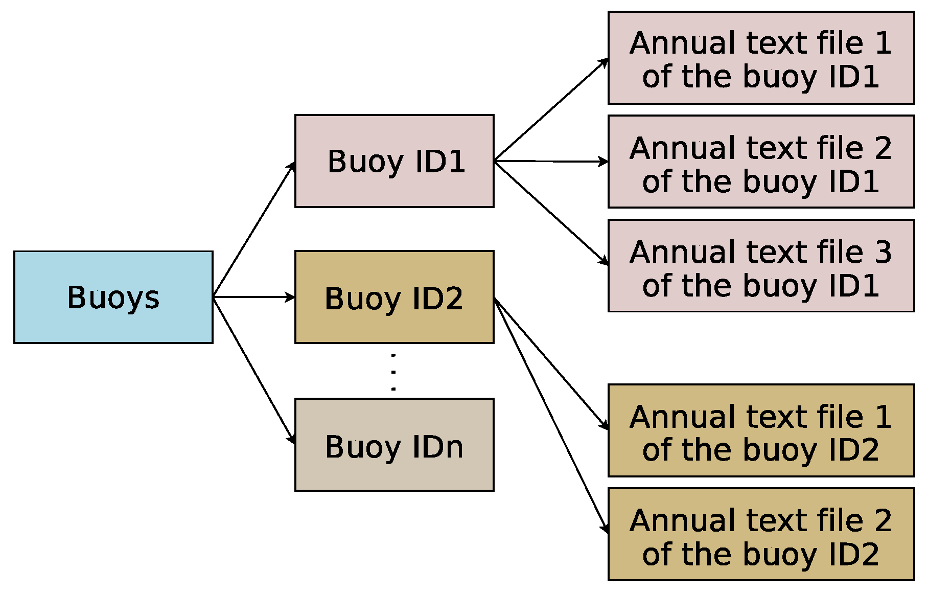
- Measurements files: The above-mentioned annual text files of the standard meteorological information recorded by the buoy and downloaded from the NDBC website. This will be used for the creation of the intermediate datasets. One file per year is expected.
3.2. Datasets
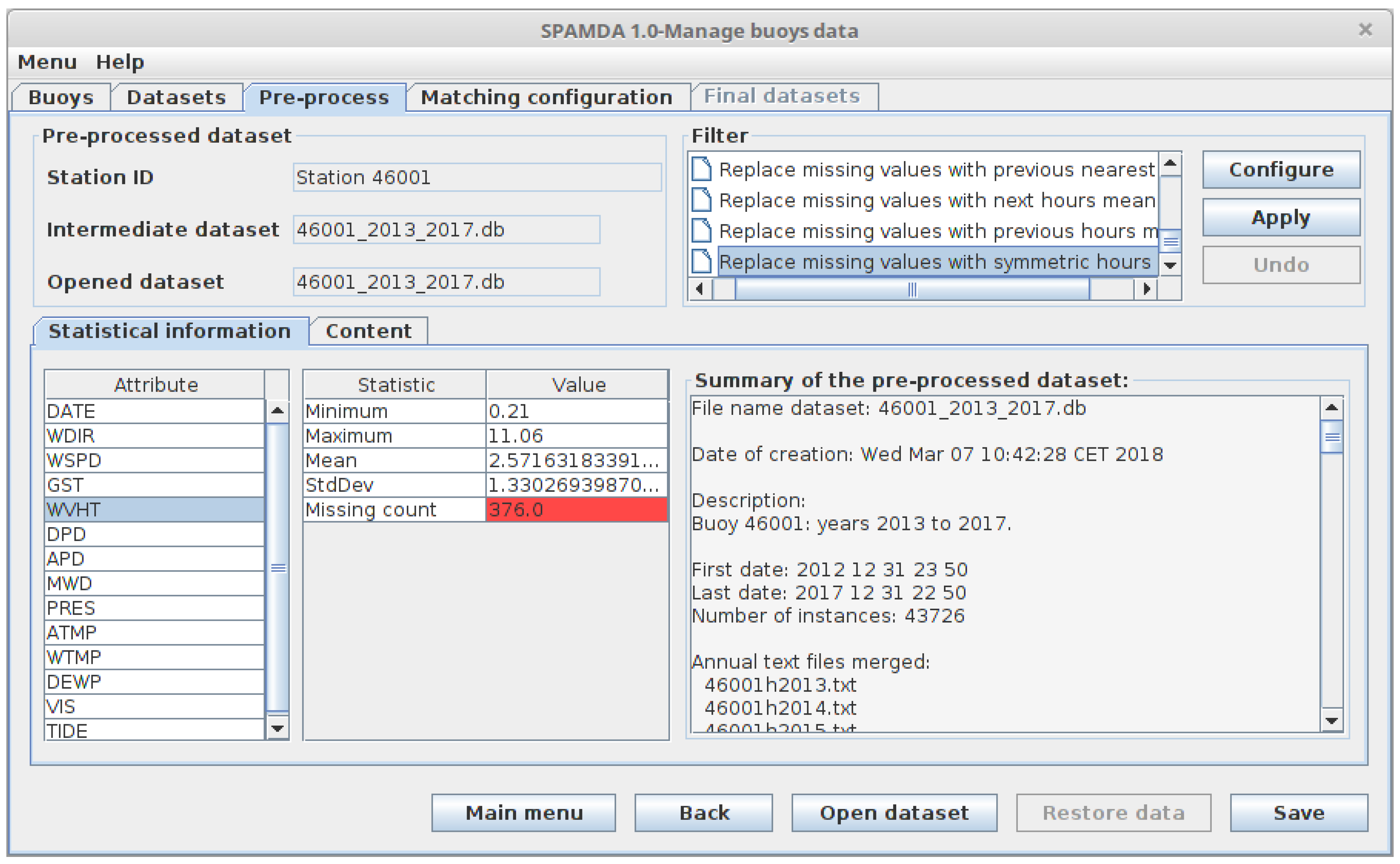
3.3. Pre-Process
- Attribute: All of these filters can be applied to the attributes (variables of the buoy from NDBC) of the intermediate dataset.
- −
- Normalize: This filter normalises all numeric values of each attribute. The resulting values are by default in the interval [0,1].
- −
- Remove: It removes an attribute or a range of them.
- −
- RemoveByName: It removes attributes based on a regular expression matched against their names.
- −
- ReplaceMissingValues: For each attribute, all the missing values will be replaced by the average value of the attribute.
- −
- ReplaceMissingWithUserConstant: This filter replaces all the missing values of the attributes with a user-supplied constant value.
- Instance: All these filters can be applied to the instances (hourly measurements of the buoy from NDBC) of the intermediate dataset.
- −
- RemoveDuplicates: With this filter, all duplicated instances are removed.
- −
- RemoveWithValues: This filter removes all the instances that match the attribute and the value supplied by the user.
- −
- SubsetByExpression: It removes all the instances that do not match a user-specified expression.
- Recover missing data: All these filters can be applied to the instances of the intermediate dataset.
- −
- Replace missing values with next nearest hour: The missing values of each attribute are replaced with the next nearest non missing value.
- −
- Replace missing values with previous nearest hour: This filter replaces the missing values of each attribute with the previous nearest non missing value.
- −
- Replace missing values with next n hours mean: The missing values of each attribute are replaced with the next n nearest non missing values mean, where n can be configured by the user.
- −
- Replace missing values with previous n hours mean: This filter replaces the missing values of each attribute in the intermediate dataset with the previous n nearest non missing values mean.
- −
- Replace missing values with symmetric n hours mean: The missing values of each attribute in the intermediate dataset are replaced with the n previous and n next non missing values mean.
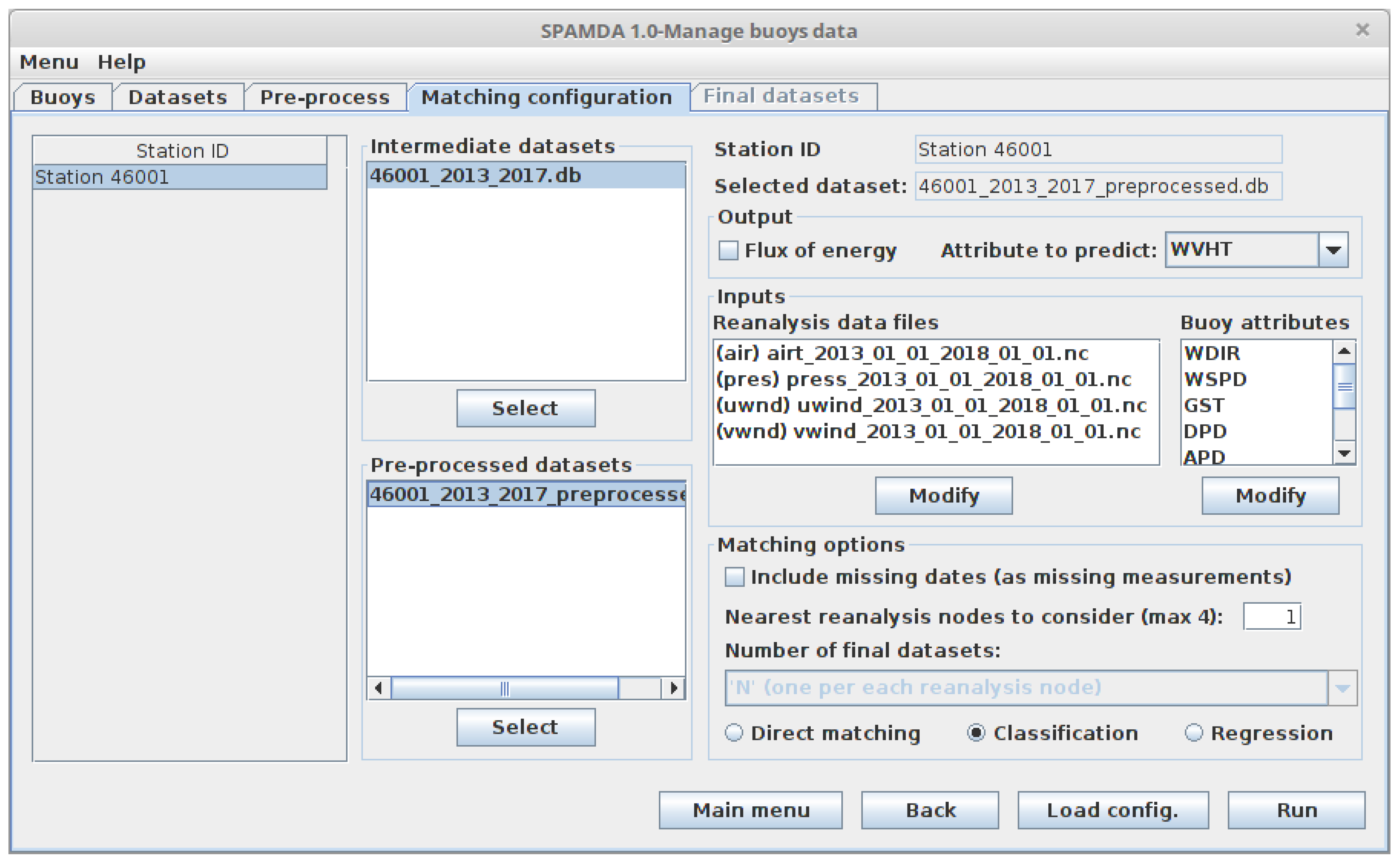
3.4. Matching Configuration
- Classification: The final datasets will be ready to use as an input for ML classifiers, requiring a nominal output attribute, whose specific preparation is detailed in Section 3.5.
- Regression: The final datasets will be ready to use as input for regression methods, requiring a real output attribute, whose preparation is also explained in Section 3.5.
- Direct matching: In this case, the inputs’ attributes have a direct correspondence with the output attribute, and it is not necessary to perform any additional preparation. Both input and target attributes are synchronised in time, in such a way that the final dataset is not intended for prediction purposes. For example, the final datasets may be used in lost data recovering tasks, in correlation studies, in descriptive analyses, etc.
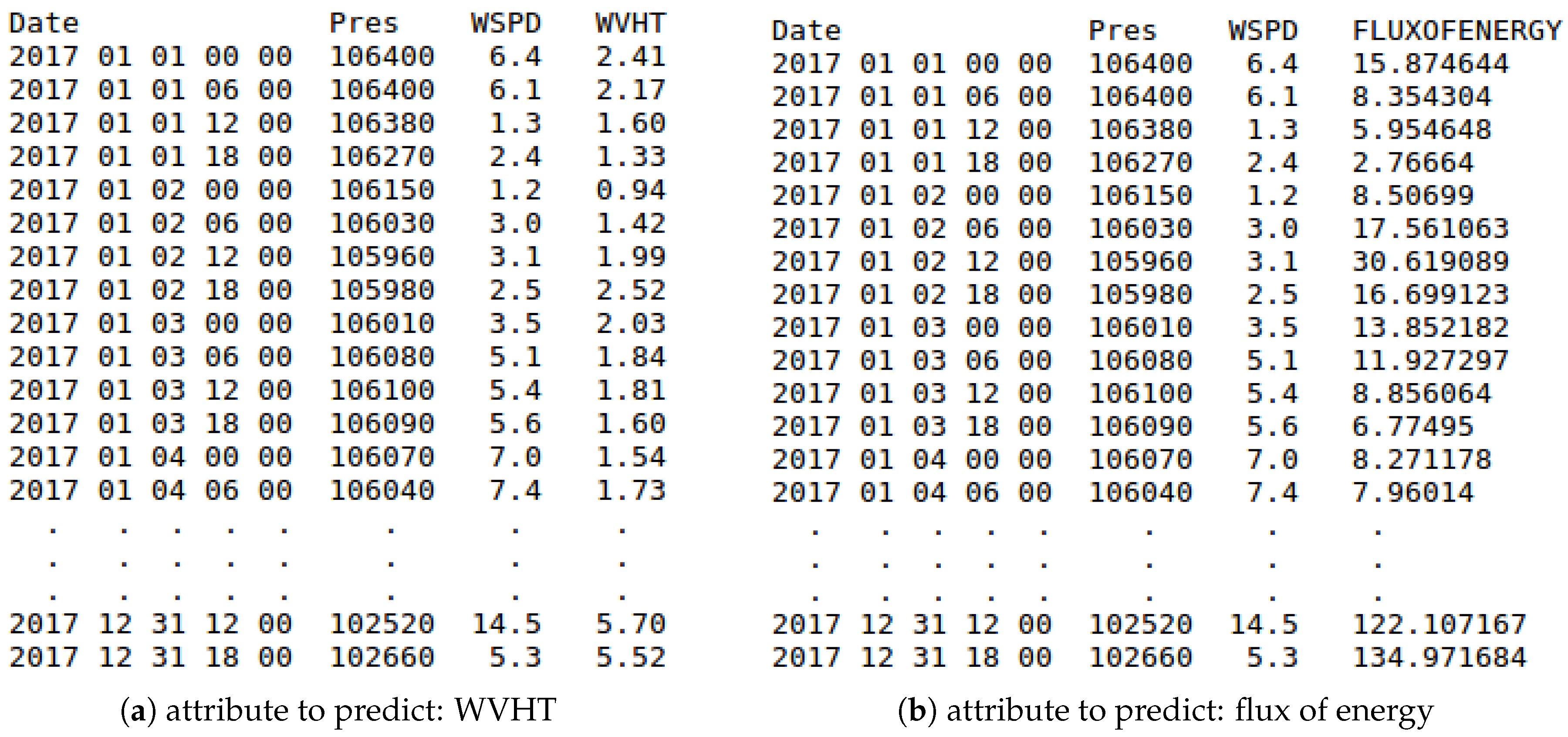
- Flux of energy [48]: When the is selected, it will be used as output. This attribute is not collected by the buoys, but there are two parameters from which it can be computed: and , which are collected as WVHT and APD attributes, respectively, and were described in Table 1. In this way, SPAMDA obtains the (measured in kilowatts per meter) of each instance using the following equation:where is measured in meters and in seconds. is referred to as flux of energy, but it is defined as an average energy flux because is an average wave height (see descriptions of the measurements on the NDBC website).
- Attribute to predict: Instead of using , researchers can select any of the attributes collected by the buoys as output (e.g., significant wave height, WVHT, wind direction, WDIR, sea level pressure, PRES, etc.). Therefore, they can conduct different studies by selecting one attribute or other.
- Reanalysis data files: In order to have a possible better description of the problem under study, more than one reanalysis variable can be considered as input. Remember that these files have to be previously downloaded from the NNRP website [61], which should set the range of dates (temporal properties) and the desired sub-grid (spatial properties, see Figure 2) for each variable of reanalysis.In that sense, the reanalysis data files must have the same spatial and temporal properties but related to different variables. SPAMDA simplifies this task by showing the reanalysis data files that are compatible with each other, and checking that the selection made by the research meets that condition.
- Buoy attributes: In addition to the reanalysis variables, the final datasets will also include the selected attributes as inputs (of the intermediate or pre-processed dataset used), providing a possible better characterisation of the problem under study, although it will depend on how correlated the attributes are.
- Include missing dates: As above-mentioned, the information collected by a buoy may be incomplete due to measurements not recorded by it. As a consequence, the matching of instances between both sources of information may not be possible (missing dates). In that situation, researchers can consider two options: (1) discard the instances affected or (2) include them. In the latter case, the final datasets will contain the affected instances, but the measurements of the buoy will be stored as missing values in WEKA format, denoted as «?».
- Nearest reanalysis nodes to consider: As already shown in Figure 2 (which represents six reanalysis nodes), the reanalysis data files may contain information of several reanalysis nodes. In this way, researchers can:
- −
- Consider all the reanalysis nodes contained in each file: in this case, the information provided by each reanalysis node contained in each selected reanalysis data file will be used.
- −
- Consider only some of the reanalysis nodes contained in each file: in this case, the information used is only that corresponding to the closest nodes to the buoy (the number of nodes, N, is indicated by the user). To do that, SPAMDA uses the Haversine equation [63] (or the great-circle distance) to calculate the distance from the location of the buoy to each node of reanalysis and obtain the closest ones. The Haversine equation performs calculation from main point to destination point with a trigonometric function:where is the geographical location of the buoy and is the position of each node. Finally, and represent the latitude and longitude of the positions of the points.
- Number of final datasets: Depending on the number of nearest reanalysis nodes to consider, the number of final datasets to create and the content of them can be configured according to the following options:
- −
- One (using weighted mean of the N nearest reanalysis nodes): Only one final dataset will be created, which will contain the attributes (the selected one as output and the selected ones as inputs) of the intermediate or pre-processed dataset used, along with a weighted mean of each variable of the reanalysis data used (one per selected reanalysis data file). This weighted mean is obtained by SPAMDA and uses Equation (2) to calculate the distance from the geographical position of the buoy to each node of reanalysis. Once the distances have been computed, they are normalised and inverted as shown in the following equation:Then, with these calculated weights, a weighted mean of each variable of reanalysis is obtained for each of the N nodes. In this way, the closest reanalysis nodes to the geographical position of the buoy will provide more information.Considering as an example the two nearest reanalysis nodes represented in Figure 2 and the reanalysis variables air temperature and pressure, the weighted mean of each reanalysis variable will be calculated using the reanalysis nodes N × W and N × W.
- −
- ‘N’ (one per each reanalysis node): As many final datasets as the number of nearest N reanalysis nodes configured by researcher will be created. Therefore, each final dataset will contain the value of each reanalysis variable used of the nearest corresponding reanalysis node, along with the selected attributes of the intermediate or pre-processed dataset used. In this way, researchers can perform comparison studies depending on the reanalysis node considered, to achieve better performance for the problem under study.In this case, and considering as example the four closest reanalysis nodes (see Figure 2) and the reanalysis variables air temperature and pressure, four final datasets will be created, each one containing the information of both reanalysis variables of the corresponding reanalysis node: N × W, N × W, N × W and N × W, along with the selected attributes of the intermediate or pre-processed dataset used.
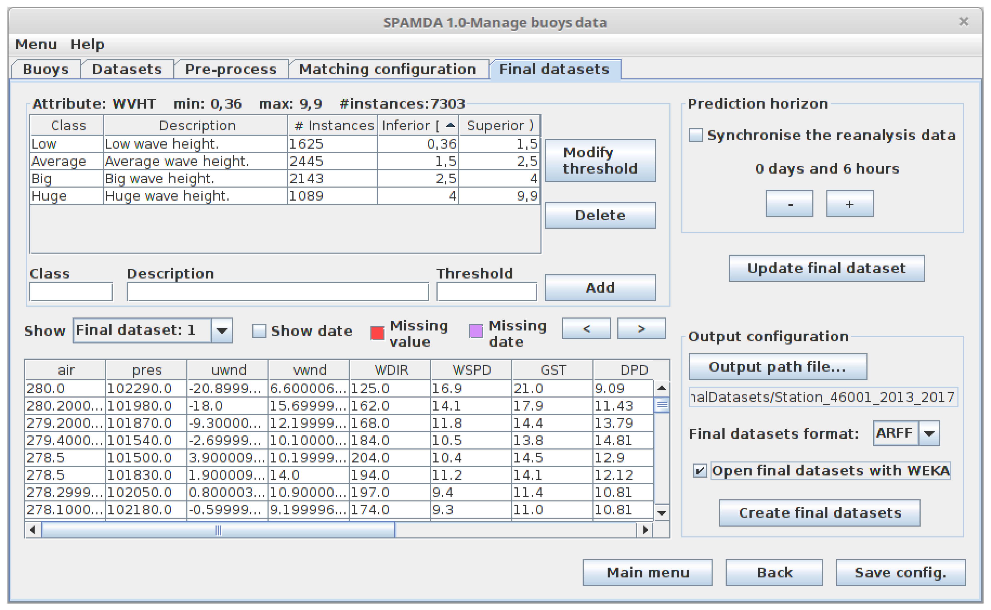
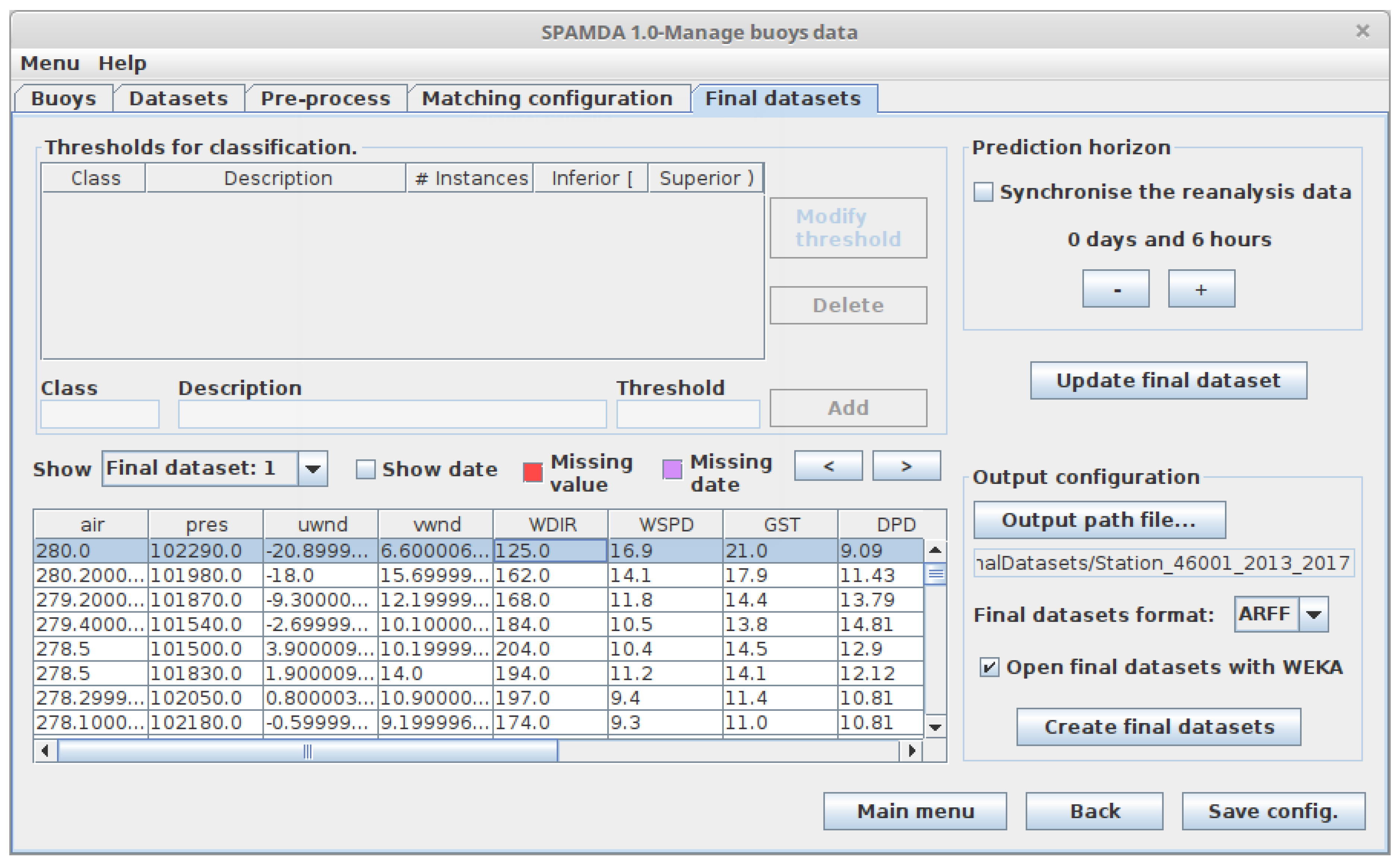
3.5. Final Datasets
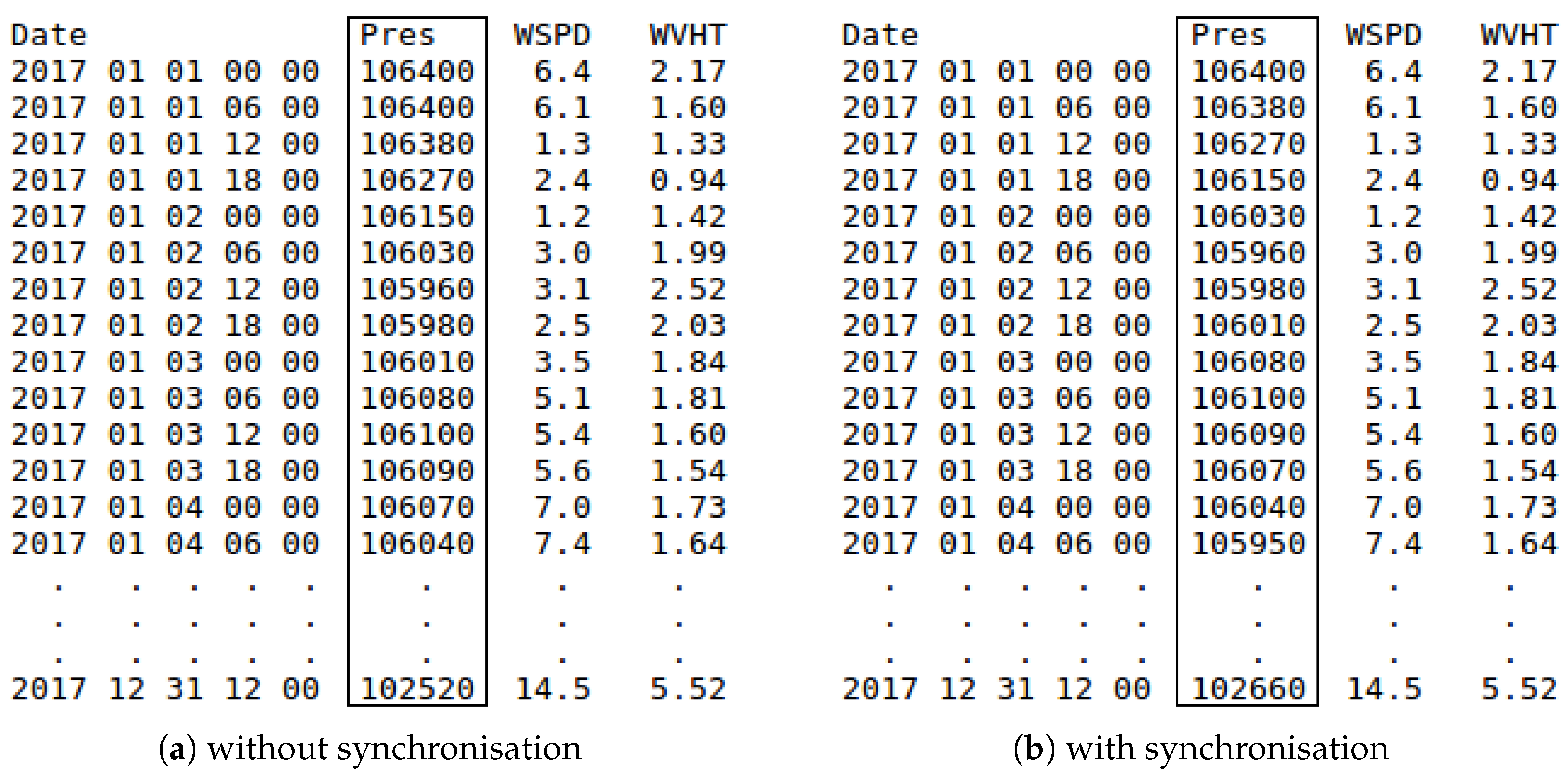
- Prediction horizon (Classification and Regression): This option indicates the time gap for moving backward the attribute to predict (output attribute). In this way, the input attributes (variables of the buoy and reanalysis data) will be used to predict the output attribute in a specific future time (e.g., +6 h, +12 h, +18 h, +1 day, etc.).The minimum interval for increasing and decreasing the prediction horizon is 6 h (due to reanalysis data temporal resolution) [4], the same interval used when the matching process is carried out. Therefore, for each increment of the prediction horizon, an instance of the dataset is lost (as this future information is not available). As the minimum prediction horizon is 6 h, at least one instance will be lost. The relation between the inputs and the output (attribute to predict) is defined as follows:where t is the time instant to study, is the prediction horizon, o is the attribute to be predicted, represents the vector that contains the selected NDBC variables, and, finally, represents the vector that contains the selected reanalysis variables. In this way and considering the matched information shown in Figure 8a, WVHT is o, the vector contains the variable WSPD, and the vector contains Pres.Optionally, the reanalysis variables can be synchronised with the attribute to predict. Given that these variables are estimated by a mathematical model, we can obtain very good future estimations, which can improve the performance of the results. In this case, the relation between the inputs and the attribute to predict would be:Note that the selected NDBC variables as input cannot be synchronised with the attribute to predict.For the sake of clarity, considering the matched information shown in Figure 8a, an example of building a dataset for a Regression task is shown in Figure 9a. As mentioned earlier, this prediction task requires a real output variable (in this case, WVHT, the last one). The options considered for the preparation of each final dataset are the following:
- −
- Do not synchronise the reanalysis data (see Equation (4) for the relation between the inputs and the output).
- −
- A prediction horizon of 6 h.
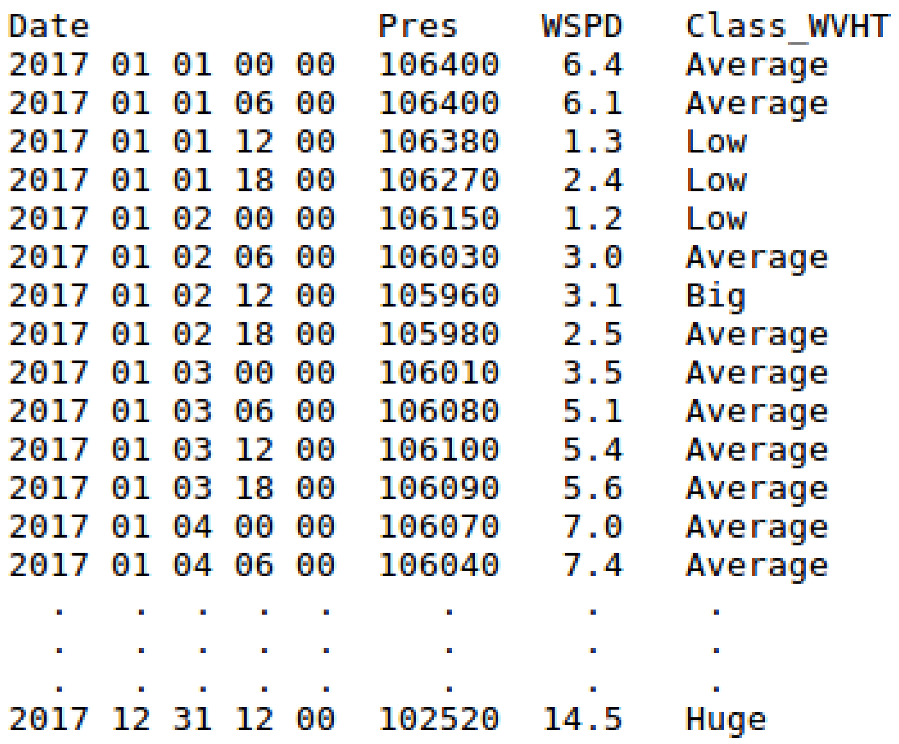
Note that, due to prediction horizon is 6 h, the values of WVHT attribute are moved backward one instance (up). As a consequence, the last instance (31 December 2017 18:00) is lost and is not included in the final dataset. In addition, and because the reanalysis data have not been synchronised, the values of the Pres and WSPD variables are at the same time instant (t in Equation (4)).Moreover, considering again the matched information shown in Figure 8a, an example of the creation of the same dataset but applying synchronisation (see Equation (5)) is shown in Figure 9b.Again, and due to the prediction horizon selected (6 h), the values of the WVHT attribute are moved backward one instance (up) and the last instance (31 December 2017 18:00) is not included in the final dataset. However, now, the values of the Pres variable are also moved backward one instance (due to the synchronisation). Therefore, in this case, Pres is at the same time instant as the attribute to predict ( in Equation (5)). - Thresholds of the output attribute (Classification): Since the values of the variables collected by the buoys are real numbers, it is necessary to discretise them (convert them from real to nominal values) for the attribute selected as output (attribute to be predicted). SPAMDA allows researchers to perform this process by defining the necessary classes with their thresholds, which will be used to carry out such discretisation.Considering again the matched information shown in Figure 8a, an example of the creation of a Classification dataset is shown in Figure 10. The options considered for the preparation of the final dataset are the following:
- −
- Do not synchronise the reanalysis data.
- −
- A prediction horizon of 6 h.
- −
- The thresholds shown in Table 2.
Note that the attribute to be predicted has been renamed to Class_WVHT to show that it is now a nominal variable because its values have been discretised according to the thresholds (usually defined by an expert). In addition, and due to the 6 h prediction horizon, the last instance is lost (31 December 2017 18:00), and the values of the attribute Class_WVHT are moved backward one instance (up). As the reanalysis data have not been synchronised, the values of the Pres and WSPD variables are at the same time instant (t in Equation (4)).
- Output path file: Name of the final datasets and folder to save them on disk.
- Final datasets format:
- −
- ARFF: Attribute-Relation File Format [53], which is used by WEKA. SPAMDA allows researchers to directly open the final datasets in the Explorer environment of WEKA (in the same context of work), enabling them to choose the most appropriate ML method to tackle the problem under study.
- −
- CSV: Comma-Separated Values. This format is included in order to consider other different tasks of software tools.
3.6. Manage Reanalysis Data
3.7. Tools
4. A Case Study Applied to Gulf of Alaska
4.1. Gathering the Information and Introducing it in SPAMDA
- The measurements obtained from 2013 to 2017 by the buoy with ID 46001, placed in the Gulf of Alaska, which are provided by NDBC as annual text files. This data are publicly available at the NDBC website.
- Complementary information collected from reanalysis data containing air temperature (air), pressure (pres) and two components of wind speed measurements, South–North (vwind) and West–East (uwind). This information can be downloaded from the NNRP website in NetCDF format for the four closest nodes of reanalysis surrounding the position of the buoy. Concretely, the closest reanalysis nodes downloaded are N × W, N × 150 W, 55 N × W, and 55 N × 150 W. However, as will be seen later, only the information from the nearest node will be used in the data integration process.
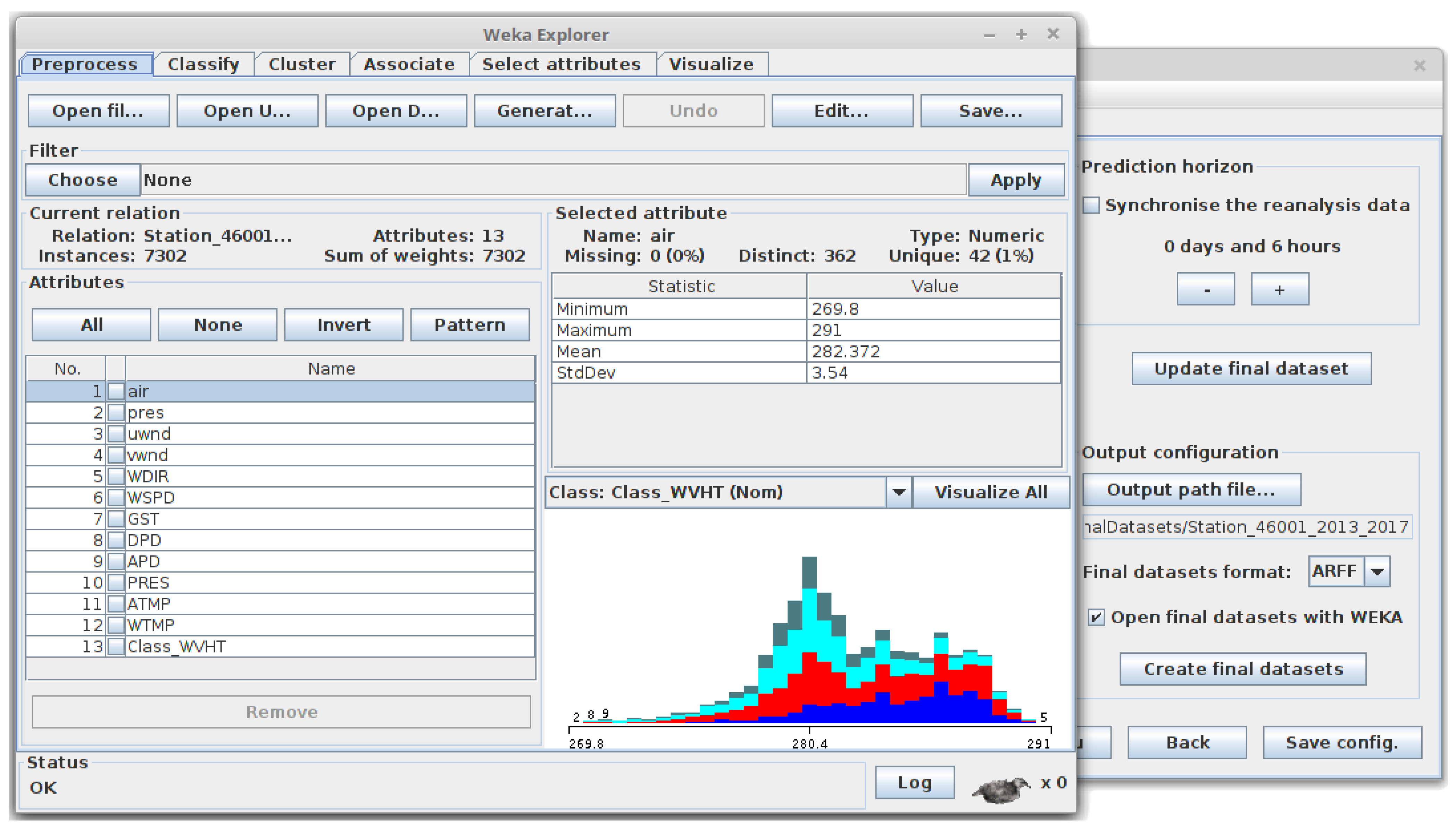
4.2. Waves Classification
4.2.1. Obtaining the Final Dataset
- Attribute to predict: WVHT.
- Reanalysis data: Air, pressure, u-wind and v-wind.
- Buoy attributes to be used as inputs: WDIR, WSPD, GST, DPD, APD, PRES, ATMP and WTMP (see Table 1 or descriptions of the measurements in the NDBC website).
- Reanalysis nodes to consider: 1 (only the closest reanalysis node will be used).
- Number of final datasets: In this example, that option is disabled because only one reanalysis node is considered.
- Prediction task: Classification.
- Thresholds: see Table 2.
- Prediction horizon: 6 h.
- Synchronisation: Disabled.
- Final dataset format: ARFF.
4.2.2. Obtaining Classification Models with ML Algorithms
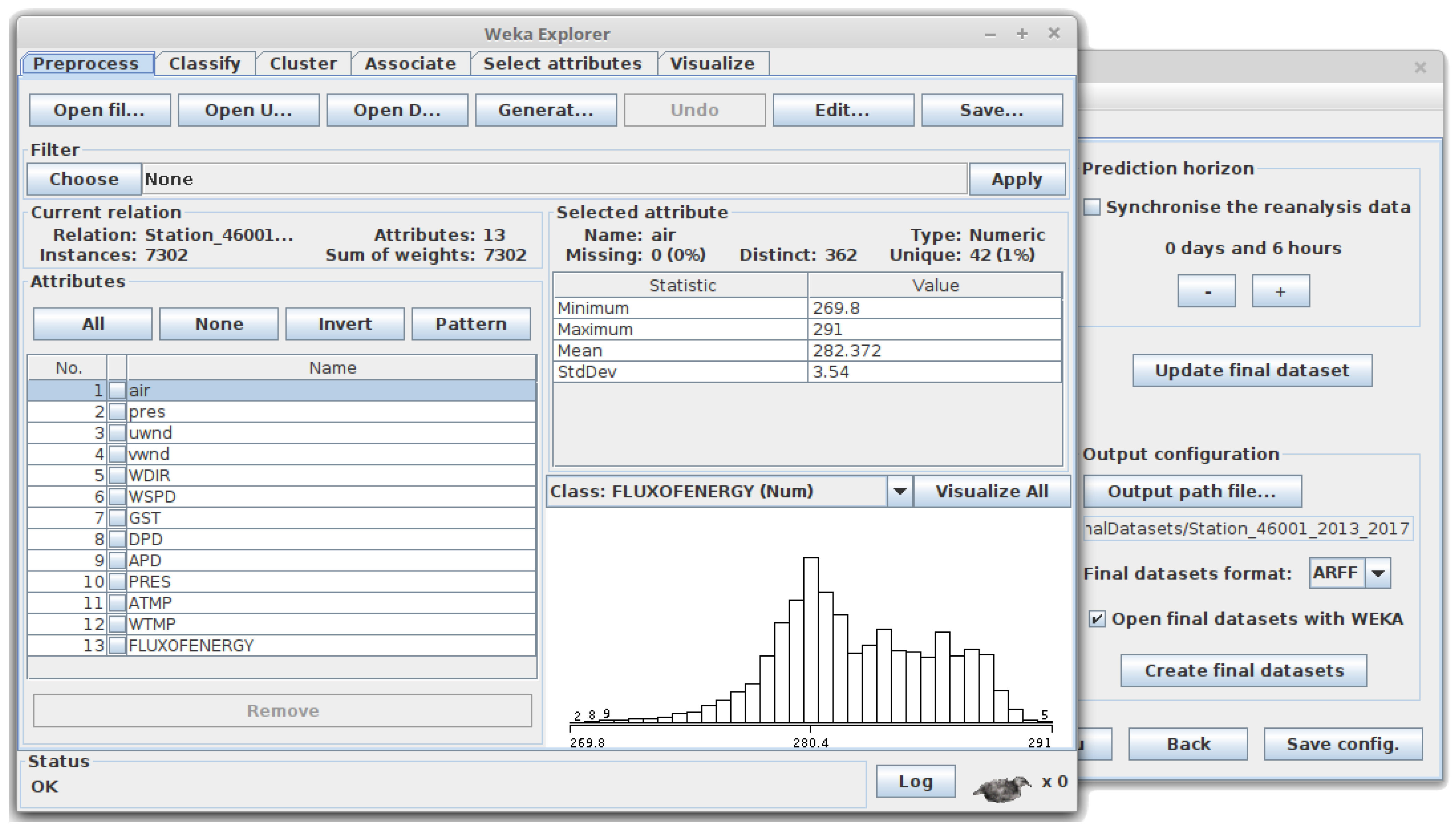
4.3. Energy Flux Prediction
4.3.1. Obtaining the Final Dataset
- Attribute to predict: Flux of energy.
- Reanalysis data: Air, pressure, u-wind and v-wind.
- Buoy attributes to be used as inputs: WDIR, WSPD, GST, DPD, APD, PRES, ATMP and WTMP (see Table 1 or descriptions of the measurements in the NDBC website).
- Reanalysis nodes to consider: 1 (only the closest reanalysis node will be used).
- Number of final datasets: In this example, this option is disabled because only one reanalysis node is considered.
- Prediction task: Regression.
- Prediction horizon: 6 h.
- Synchronisation: Disabled.
- Final dataset format: ARFF.
4.3.2. Obtaining Prediction Models with ML Algorithms
4.4. Important Remarks
5. Conclusions
Supplementary Materials
Author Contributions
Funding
Institutional Review Board Statement
Informed Consent Statement
Data Availability Statement
Acknowledgments
Conflicts of Interest
Abbreviations
| Flux of energy | |
| Significant wave height | |
| Wave energy period | |
| Geographical location of the buoy | |
| Geographical location of each reanalysis node | |
| Latitude of the point | |
| Longitude of the point | |
| The attribute to be predicted at the time instant to study | |
| The prediction horizon | |
| The vector containing the selected NDBC variables | |
| The vector containing the selected reanalysis variables |
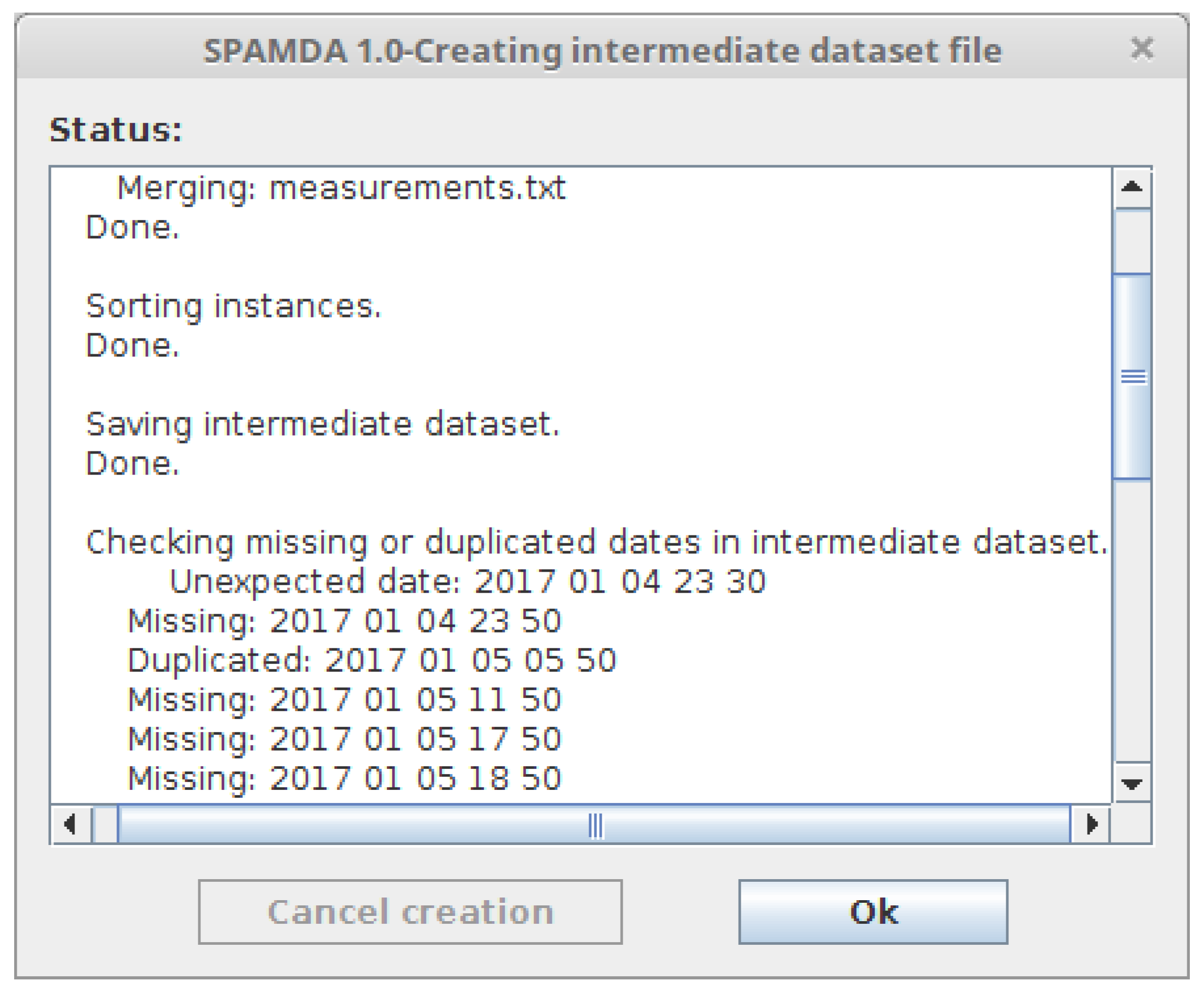
Appendix A. Managing the Casuistry of Incomplete Data
- In the instance marked with (a), the measurement of 17:50 was collected at 17:45, 5 min earlier.
- In the instance marked with (b), the measurement of 23:50 was collected at 23:30, 20 min earlier.
- In the instance marked with (c), the measurement of 05:50 is duplicated.
- In the instance marked with (d), the measurement of 11:50 is missing (missing date or instance).
- In the instance marked with (e), the measurement of 17:50 and 18:50 are missing (missing dates or instances).
- Missing values highlighted in red.


References
- Anis, M.S.; Jamil, B.; Ansari, M.A.; Bellos, E. Generalized models for estimation of global solar radiation based on sunshine duration and detailed comparison with the existing: A case study for India. Sustain. Energy Technol. Assess. 2019, 31, 179–198. [Google Scholar] [CrossRef]
- Laface, V.; Arena, F.; Soares, C.G. Directional analysis of sea storms. Ocean Eng. 2015, 107, 45–53. [Google Scholar] [CrossRef]
- Shivam, K.; Tzou, J.C.; Wu, S.C. Multi-Objective Sizing Optimization of a Grid-Connected Solar–Wind Hybrid System Using Climate Classification: A Case Study of Four Locations in Southern Taiwan. Energies 2020, 13, 2505. [Google Scholar] [CrossRef]
- Dorado-Moreno, M.; Cornejo-Bueno, L.; Gutiérrez, P.A.; Prieto, L.; Hervás-Martínez, C.; Salcedo-Sanz, S. Robust estimation of wind power ramp events with reservoir computing. Renew. Energy 2017, 111, 428–437. [Google Scholar] [CrossRef]
- He, Q.; Zha, C.; Song, W.; Hao, Z.; Du, Y.; Liotta, A.; Perra, C. Improved Particle Swarm Optimization for Sea Surface Temperature Prediction. Energies 2020, 13, 1369. [Google Scholar] [CrossRef]
- Fuchs, H.L.; Gerbi, G.P. Seascape-level variation in turbulence- and wave-generated hydrodynamic signals experienced by plankton. Prog. Oceanogr. 2016, 141, 109–129. [Google Scholar] [CrossRef]
- Da Silva, V.D.P.R.; Araújo e Silva, R.; Cavalcanti, E.P.; Braga Campos, C.; Vieira de Azevedo, P.; Singh, V.P.; Rodrigues Pereira, E.R. Trends in solar radiation in NCEP/NCAR database and measurements in northeastern Brazil. Sol. Energy 2010, 84, 1852–1862. [Google Scholar] [CrossRef]
- Gouldby, B.; Méndez, F.J.; Guanche, Y.; Rueda, A.; Mínguez, R. A methodology for deriving extreme nearshore sea conditions for structural design and flood risk analysis. Coast. Eng. 2014, 88, 15–26. [Google Scholar] [CrossRef]
- Alizadeh, R.; Jia, L.; Nellippallil, A.B.; Wang, G.; Hao, J.; Allen, J.K.; Mistree, F. Ensemble of surrogates and cross-validation for rapid and accurate predictions using small data sets. Artif. Intell. Eng. Des. Anal. Manuf. 2019, 33, 484–501. [Google Scholar] [CrossRef]
- Alizadeh, R.; Allen, J.K.; Mistree, F. Managing computational complexity using surrogate models: A critical review. Res. Eng. Des. 2020, 31, 275–298. [Google Scholar] [CrossRef]
- Manfren, M.; Groppi, D.; Astiaso Garcia, D. Open data and energy analytics—An analysis of essential information for energy system planning, design and operation. Energies 2020, 13, 2334. [Google Scholar] [CrossRef]
- Dhanraj Bokde, N.; Mundher Yaseen, Z.; Bruun Andersen, G. ForecastTB—An R Package as a Test-Bench for Time Series Forecasting—Application of Wind Speed and Solar Radiation Modeling. Energies 2020, 13, 2578. [Google Scholar] [CrossRef]
- Lo, C.K.; Lim, Y.S.; Rahman, F.A. New integrated simulation tool for the optimum design of bifacial solar panel with reflectors on a specific site. Renew. Energy 2015, 81, 293–307. [Google Scholar] [CrossRef]
- Nguyen, T.H.; Prinz, A.; Friisø, T.; Nossum, R.; Tyapin, I. A framework for data integration of offshore wind farms. Renew. Energy 2013, 60, 150–161. [Google Scholar] [CrossRef]
- Di Bari, R.; Horn, R.; Nienborg, B.; Klinker, F.; Kieseritzky, E.; Pawelz, F. The Environmental Potential of Phase Change Materials in Building Applications. A Multiple Case Investigation Based on Life Cycle Assessment and Building Simulation. Energies 2020, 13, 3045. [Google Scholar] [CrossRef]
- Astiaso Garcia, D.; Bruschi, D. A risk assessment tool for improving safety standards and emergency management in Italian onshore wind farms. Sustain. Energy Technol. Assess. 2016, 18, 48–58. [Google Scholar] [CrossRef]
- Raabe, A.L.A.; Klein, A.H.d.F.; González, M.; Medina, R. MEPBAY and SMC: Software tools to support different operational levels of headland-bay beach in coastal engineering projects. Coast. Eng. 2010, 57, 213–226. [Google Scholar] [CrossRef]
- Motahhir, S.; EL Hammoumi, A.; EL Ghzizal, A.; Derouich, A. Open hardware/software test bench for solar tracker with virtual instrumentation. Sustain. Energy Technol. Assess. 2019, 31, 9–16. [Google Scholar] [CrossRef]
- Cascajo, R.; García, E.; Quiles, E.; Correcher, A.; Morant, F. Integration of Marine Wave Energy Converters into Seaports: A Case Study in the Port of Valencia. Energies 2019, 12, 787. [Google Scholar] [CrossRef]
- Zeyringer, M.; Fais, B.; Keppo, I.; Price, J. The potential of marine energy technologies in the UK—Evaluation from a systems perspective. Renew. Energy 2018, 115, 1281–1293. [Google Scholar] [CrossRef]
- De Jong, M.; Hoppe, T.; Noori, N. City Branding, Sustainable Urban Development and the Rentier State. How do Qatar, Abu Dhabi and Dubai present Themselves in the Age of Post Oil and Global Warming? Energies 2019, 12, 1657. [Google Scholar] [CrossRef]
- Brede, M.; de Vries, B.J.M. The energy transition in a climate-constrained world: Regional vs. global optimization. Environ. Model. Softw. 2013, 44, 44–61. [Google Scholar] [CrossRef]
- Alizadeh, R.; Lund, P.D.; Soltanisehat, L. Outlook on biofuels in future studies: A systematic literature review. Renew. Sustain. Energy Rev. 2020, 134, 110326. [Google Scholar] [CrossRef]
- Falcão, A.F.D.O. Wave energy utilization: A review of the technologies. Renew. Sustain. Energy Rev. 2010, 14, 899–918. [Google Scholar] [CrossRef]
- Amini, E.; Golbaz, D.; Amini, F.; Majidi Nezhad, M.; Neshat, M.; Astiaso Garcia, D. A Parametric Study of Wave Energy Converter Layouts in Real Wave Models. Energies 2020, 13, 6095. [Google Scholar] [CrossRef]
- Oliveira-Pinto, S.; Rosa-Santos, P.; Taveira-Pinto, F. Electricity supply to offshore oil and gas platforms from renewable ocean wave energy: Overview and case study analysis. Energy Convers. Manag. 2019, 186, 556–569. [Google Scholar] [CrossRef]
- Fernández Prieto, L.; Rodríguez Rodríguez, G.; Schallenberg Rodríguez, J. Wave energy to power a desalination plant in the north of Gran Canaria Island: Wave resource, socioeconomic and environmental assessment. J. Environ. Manag. 2019, 231, 546–551. [Google Scholar] [CrossRef]
- Ochi, M.K. Ocean Waves: The Stochastic Approach; Cambridge Ocean Technology Series; Cambridge University Press: Cambridge, UK, 1998. [Google Scholar]
- Crowley, S.; Porter, R.; Taunton, D.J.; Wilson, P.A. Modelling of the WITT wave energy converter. Renew. Energy 2018, 115, 159–174. [Google Scholar] [CrossRef]
- Abdelkhalik, O.; Robinett, R.; Zou, S.; Bacelli, G.; Coe, R.; Bull, D.; Wilson, D.; Korde, U. On the control design of wave energy converters with wave prediction. J. Ocean. Eng. Mar. Energy 2016, 2, 473–483. [Google Scholar] [CrossRef]
- Ringwood, J.V.; Bacelli, G.; Fusco, F. Energy-Maximizing Control of Wave-Energy Converters: The Development of Control System Technology to Optimize Their Operation. IEEE Control Syst. 2014, 34, 30–55. [Google Scholar] [CrossRef]
- Wei, C.C. Nearshore Wave Predictions Using Data Mining Techniques during Typhoons: A Case Study near Taiwan’s Northeastern Coast. Energies 2018, 11, 11. [Google Scholar] [CrossRef]
- Kaloop, M.R.; Kumar, D.; Zarzoura, F.; Roy, B.; Hu, J.W. A wavelet—Particle swarm optimization—Extreme learning machine hybrid modeling for significant wave height prediction. Ocean Eng. 2020, 213, 107777. [Google Scholar] [CrossRef]
- Rusu, L. Assessment of the Wave Energy in the Black Sea Based on a 15-Year Hindcast with Data Assimilation. Energies 2015, 8, 10370–10388. [Google Scholar] [CrossRef]
- Rhee, S.Y.; Park, J.; Inoue, A. (Eds.) Soft Computing in Machine Learning; Springer: Berlin, Germany, 2014. [Google Scholar]
- Bishop, C.M. Pattern Recognition and Machine Learning; Springer: New York, NY, USA, 2006. [Google Scholar]
- Chang, F.J.; Hsu, K.; Chang, L.C. (Eds.) Flood Forecasting Using Machine Learning Methods; MPDI: Basel, Switzerland, 2019. [Google Scholar]
- Dineva, A.; Mosavi, A.; Faizollahzadeh Ardabili, S.; Vajda, I.; Shamshirband, S.; Rabczuk, T.; Chau, K.W. Review of Soft Computing Models in Design and Control of Rotating Electrical Machines. Energies 2019, 12, 1049. [Google Scholar] [CrossRef]
- Guo, Y.; Wang, J.; Chen, H.; Li, G.; Liu, J.; Xu, C.; Huang, R.; Huang, Y. Machine learning-based thermal response time ahead energy demand prediction for building heating systems. Appl. Energy 2018, 221, 16–27. [Google Scholar] [CrossRef]
- Frank, E.; Hall, M.A.; Witten, I.H. The WEKA Workbench. Online Appendix for Data Mining: Practical Machine Learning Tools and Techniques; Morgan Kaufmann: Cambridge, MA, USA, 2016. [Google Scholar]
- Durán-Rosal, A.M.; Fernández, J.C.; Gutiérrez, P.A.; Hervás-Martínez, C. Detection and prediction of segments containing extreme significant wave heights. Ocean Eng. 2017, 142, 268–279. [Google Scholar] [CrossRef]
- Kumar, N.K.; Savitha, R.; Al Mamun, A. Regional ocean wave height prediction using sequential learning neural networks. Ocean Eng. 2017, 129, 605–612. [Google Scholar] [CrossRef]
- Ali, M.; Prasad, R.; Xiang, Y.; Deo, R.C. Near real-time significant wave height forecasting with hybridized multiple linear regression algorithms. Renew. Sustain. Energy Rev. 2020, 132, 110003. [Google Scholar] [CrossRef]
- Cornejo-Bueno, L.; Nieto-Borge, J.; García-Díaz, P.; Rodríguez, G.; Salcedo-Sanz, S. Significant wave height and energy flux prediction for marine energy applications: A grouping genetic algorithm—Extreme Learning Machine approach. Renew. Energy 2016, 97, 380–389. [Google Scholar] [CrossRef]
- Emmanouil, S.; Aguilar, S.G.; Nane, G.F.; Schouten, J.J. Statistical models for improving significant wave height predictions in offshore operations. Ocean Eng. 2020, 206, 107249. [Google Scholar] [CrossRef]
- Shamshirband, S.; Mosavi, A.; Rabczuk, T.; Nabipour, N.; Wing Chau, K. Prediction of significant wave height; comparison between nested grid numerical model, and machine learning models of artificial neural networks, extreme learning and support vector machines. Eng. Appl. Comput. Fluid Mech. 2020, 14, 805–817. [Google Scholar] [CrossRef]
- Johansson, L.; Epitropou, V.; Karatzas, K.; Karppinen, A.; Wanner, L.; Vrochidis, S.; Bassoukos, A.; Kukkonen, J.; Kompatsiaris, I. Fusion of meteorological and air quality data extracted from the web for personalized environmental information services. Environ. Model. Softw. 2015, 64, 143–155. [Google Scholar] [CrossRef]
- Fernández, J.C.; Salcedo-Sanz, S.; Gutiérrez, P.A.; Alexandre, E.; Hervás-Martínez, C. Significant wave height and energy flux range forecast with machine learning classifiers. Eng. Appl. Artif. Intell. 2015, 43, 44–53. [Google Scholar] [CrossRef]
- Adams, J.; Flora, S. Correlating seabird movements with ocean winds: Linking satellite telemetry with ocean scatterometry. Mar. Biol. 2010, 157, 915–929. [Google Scholar] [CrossRef]
- National Data Buoy Center. National Oceanic and Atmospheric Administration of the USA (NOAA). Available online: http://www.ndbc.noaa.gov/ (accessed on 10 December 2020).
- Kalnay, E.; Kanamitsu, M.; Kistler, R.; Collins, W.; Deaven, D.; Gandin, L.; Iredell, M.; Saha, S.; White, G.; Woollen, J.; et al. The NCEP/NCAR 40-Year Reanalysis Project. Bull. Am. Meteorol. Soc. 1996, 77, 437–471. [Google Scholar] [CrossRef]
- Kistler, R.; Collins, W.; Saha, S.; White, G.; Woollen, J.; Kalnay, E.; Chelliah, M.; Ebisuzaki, W.; Kanamitsu, M.; Kousky, V.; et al. The NCEP–NCAR 50–Year Reanalysis: Monthly Means CD–ROM and Documentation. Bull. Am. Meteorol. Soc. 2001, 82, 247–267. [Google Scholar] [CrossRef]
- The WEKA Data Mining Software: Attribute-Relation File Format (ARFF). Available online: https://www.cs.waikato.ac.nz/ml/weka/arff.html (accessed on 10 December 2020).
- Ali, M.; Prasad, R. Significant wave height forecasting via an extreme learning machine model integrated with improved complete ensemble empirical mode decomposition. Renew. Sustain. Energy Rev. 2019, 104, 281–295. [Google Scholar] [CrossRef]
- Chatziioannou, K.; Katsardi, V.; Koukouselis, A.; Mistakidis, E. The effect of nonlinear wave-structure and soil-structure interactions in the design of an offshore structure. Mar. Struct. 2017, 52, 126–152. [Google Scholar] [CrossRef]
- Dalgic, Y.; Lazakis, I.; Dinwoodie, I.; McMillan, D.; Revie, M. Advanced logistics planning for offshore wind farm operation and maintenance activities. Ocean Eng. 2015, 101, 211–226. [Google Scholar] [CrossRef]
- Spaulding, M.L.; Grilli, A.; Damon, C.; Crean, T.; Fugate, G.; Oakley, B.A.; Stempel, P. STORMTOOLS: Coastal Environmental Risk Index (CERI). J. Mar. Sci. Eng. 2016, 4, 54. [Google Scholar] [CrossRef]
- National Data Buoy Center. NDBC—Historical NDBC Data. Available online: http://www.ndbc.noaa.gov/historical_data.shtml (accessed on 10 December 2020).
- National Data Buoy Center. NDBC—Important NDBC Web Site Changes. Available online: http://www.ndbc.noaa.gov/mods.shtml (accessed on 10 December 2020).
- National Data Buoy Center. Measurement Descriptions and Units. Available online: https://www.ndbc.noaa.gov/measdes.shtml#stdmet (accessed on 10 December 2020).
- NOAA/OAR/ESRL PSD. ESRL : PSD : NCEP/NCAR Reanalysis 1. Available online: https://www.esrl.noaa.gov/psd/data/gridded/data.ncep.reanalysis.html (accessed on 15 January 2019).
- Unidata. Network Common Data Form (NetCDF) Version 4.6.10 [Software]; UCAR/Unidata: Boulder, CO, USA, 2017. [Google Scholar] [CrossRef]
- De Smith, M.J.; Goodchild, M.F.; Longley, P.A. Geospatial Analysis: A Comprehensive Guide to Principles, Techniques and Software Tools, 3rd ed.; Matador: Leicester, UK, 2009. [Google Scholar]
- Hosmer, D.W., Jr.; Lemeshow, S.; Sturdivant, R.X. Applied Logistic Regression, 3rd ed.; John Wiley & Sons: Hoboken, NJ, USA, 2013. [Google Scholar]
- Quinlan, J.R. C4. 5: Programs for Machine Learning; Morgan Kaufmann: Burlington, MA, USA, 1992. [Google Scholar]
- Breiman, L. Random forests. Mach. Learn. 2001, 45, 5–32. [Google Scholar] [CrossRef]
- Cortes, C.; Vapnik, V. Support-vector networks. Mach. Learn. 1995, 20, 273–297. [Google Scholar] [CrossRef]
- Haykin, S. Neural Networks: A Comprehensive Foundation; Prentice Hall PTR: Hoboken, NJ, USA, 1994. [Google Scholar]
- National Data Buoy Center. NDBC—Measurement Descriptions and Units. Available online: https://www.ndbc.noaa.gov/measdes.shtml (accessed on 10 December 2020).
- Durán-Rosal, A.M.; Hervás-Martínez, C.; Tallón-Ballesteros, A.J.; Martínez-Estudillo, A.C.; Salcedo-Sanz, S. Massive missing data reconstruction in ocean buoys with evolutionary product unit neural networks. Ocean Eng. 2016, 117, 292–301. [Google Scholar] [CrossRef]
- Alcalá-Fdez, J.; Sánchez, L.; García, S.; del Jesús, M.J.; Ventura, S.; Garrell, J.M.; Otero, J.; Romero, C.; Bacardit, J.; Rivas, V.M.; et al. KEEL: A software tool to assess evolutionary algorithms for data mining problems. Soft Comput. 2009, 13, 307–318. [Google Scholar] [CrossRef]


| Attribute | Units | Description |
|---|---|---|
| WDIR | degT | The direction the wind is coming from true North. |
| WSPD | m/s | The speed of the wind. |
| GST | m/s | Peak of gust speed. |
| WVHT | m | Significant wave height. |
| DPD | sec | Dominant wave period (maximum wave energy). |
| APD | sec | Average wave period of all waves. |
| MWD | degT | The direction from which the waves at the dominant period are coming. |
| PRES | hPa | Sea level pressure. |
| ATMP | degC | Air temperature. |
| WTMP | degC | Sea surface temperature. |
| DEWP | degC | Dewpoint temperature. |
| VIS | nmi | Visibility of the station. |
| TIDE | ft | The water level. |
| Class | Description | Lower End [ | Upper End ) |
|---|---|---|---|
| Low | Low wave height | ||
| Average | Average wave height | ||
| Big | Big wave height | ||
| Huge | Huge wave height |
| Year | Number of Instances |
|---|---|
| 2013 | 1460 |
| 2014 | 1460 |
| 2015 | 1460 |
| 2016 | 1464 |
| 2017 | 1458 |
| 7302 |
| Algorithm | Accuracy (CCR) | Kappa |
|---|---|---|
| Logistic Regression | ||
| C4.5 | ||
| Random Forest | ||
| Support Vector Machine | ||
| Multilayer Perceptron |
| Algorithm | Root Mean Squared Error | Correlation Coefficient |
|---|---|---|
| Linear Regression | ||
| Random Forest | ||
| Support Vector Machine | ||
| Multilayer Perceptron |
Publisher’s Note: MDPI stays neutral with regard to jurisdictional claims in published maps and institutional affiliations. |
© 2021 by the authors. Licensee MDPI, Basel, Switzerland. This article is an open access article distributed under the terms and conditions of the Creative Commons Attribution (CC BY) license (http://creativecommons.org/licenses/by/4.0/).
Share and Cite
Gómez-Orellana, A.M.; Fernández, J.C.; Dorado-Moreno, M.; Gutiérrez, P.A.; Hervás-Martínez, C. Building Suitable Datasets for Soft Computing and Machine Learning Techniques from Meteorological Data Integration: A Case Study for Predicting Significant Wave Height and Energy Flux. Energies 2021, 14, 468. https://doi.org/10.3390/en14020468
Gómez-Orellana AM, Fernández JC, Dorado-Moreno M, Gutiérrez PA, Hervás-Martínez C. Building Suitable Datasets for Soft Computing and Machine Learning Techniques from Meteorological Data Integration: A Case Study for Predicting Significant Wave Height and Energy Flux. Energies. 2021; 14(2):468. https://doi.org/10.3390/en14020468
Chicago/Turabian StyleGómez-Orellana, Antonio Manuel, Juan Carlos Fernández, Manuel Dorado-Moreno, Pedro Antonio Gutiérrez, and César Hervás-Martínez. 2021. "Building Suitable Datasets for Soft Computing and Machine Learning Techniques from Meteorological Data Integration: A Case Study for Predicting Significant Wave Height and Energy Flux" Energies 14, no. 2: 468. https://doi.org/10.3390/en14020468
APA StyleGómez-Orellana, A. M., Fernández, J. C., Dorado-Moreno, M., Gutiérrez, P. A., & Hervás-Martínez, C. (2021). Building Suitable Datasets for Soft Computing and Machine Learning Techniques from Meteorological Data Integration: A Case Study for Predicting Significant Wave Height and Energy Flux. Energies, 14(2), 468. https://doi.org/10.3390/en14020468