Optimal Control of Wind Turbine Systems via Time-Scale Decomposition

Abstract

In this paper, we design an optimal controller for a wind turbine (WT) with doubly-fed induction generator (DFIG) by decomposing the algebraic Riccati equation (ARE) of the singularly perturbed wind turbine system into two reduced-order AREs that correspond to the slow and fast time scales. In addition, we derive a mathematical expression to obtain the optimal regulator gains with respect to the optimal pure-slow and pure-fast, reduced-order Kalman filters and linear quadratic Gaussian (LQG) controllers. Using this method allows the design of the linear controllers for slow and fast subsystems independently, thus, achieving complete separation and parallelism in the design process. This solves the corresponding ill-conditioned problem and reduces the complexity that arises when the number of wind turbines integrated to the power system increases. The reduced-order systems are compared to the original full-order system to validate the performance of the proposed method when a wind turbulence and a large-signal disturbance are applied to the system. In addition, we show that the similarity transformation does not preserve the performance index value in case of Kalman filter and the corresponding LQG controller.

1. Introduction

Wind turbines, having mechanical and electrical components, are known to operate in at least two time-scales: the slow time scale in which mechanical state variables evolve and the fast time scale in which electrical and electronic state variables evolve. The result is the “stiff” numerical problem that happens naturally in power systems due to the presence of “parasitic” parameters such as small time constants, masses, resistances, inductances, capacitances, moments of inertia, etc. Singular perturbation methods eliminate the stiffness problem and decouple the original system into slow and fast reduced-order subsystems. A reduced-order system can be obtained through ignoring the fast subsystem and compensating for its effect by introducing a “boundary layer” correction to the slow subsystem towards a better approximation for the original system. Various methods have been proposed [1,2] to obtain the exact slow and fast subsystems. The Chang transformation [3] has been widely used to get the exact pure-slow and pure-fast subsystems, even when the perturbation parameter $ϵ$ is not very small. Moreover, a number of recursive algorithms [4,5,6] have been developed to avoid the problems involving ill-conditioned systems and to obtain an approximate solution to the algebraic Riccati equation (ARE), which can be decomposed after that into slow and fast parts.

Double-Fed Induction Generators (DFIGs) are characterized by consuming less reactive power, inflicting less mechanical stress on turbines, and allowing the control of the active and reactive power to be decoupled. As such, DFIGs are commonly used in variable-speed wind energy systems [7]. However, due to their poorly damped eigenvalues, modeling and control of DFIG-based wind systems is more complicated than that of other induction generators. This is further exacerbated by the sensitivity of DFIGs to grid disturbances, which may, under certain operating conditions, render the system unstable [8].

Time scale analysis and optimal control of wind energy systems have been widely explored [9,10,11,12,13,14]. Using time scale analysis, in [9] the linear quadratic regulator (LQR) and LQG controllers were designed for deterministic and stochastic wind energy systems with permanent magnet synchronous generators (PMSG). In [10], the LQR controller was designed for a DFIG wind turbine and compared to current-mode control under different types of disturbances affecting the wind turbine system. The LQR controller is used in [11] for the pitch angle control, and in [12] to control the oscillatory behavior towards improving the stability, of the DFIG connected to the grid. In comparison to the balanced reduction methods in [13], time scale and singular perturbation analysis provide better results in reducing the order of the DFIG-based WT system. A LQG-based power oscillation damping controller is designed in [14] to provide the supplementary reference signals for the active and reactive power of the DFIG wind generator and to enhance the damping of poorly damped modes.

In this paper, the method of singular perturbation will be used to design LQR, Kalman filter, and LQG optimal controllers in two independent time scales for a fifth-order single-cage DFIG wind turbine. Here, the ARE of the singularly perturbed wind turbine system is decomposed into two reduced-order AREs that correspond to the slow and fast time scales. Using this method allows designing linear controllers for the slow and fast subsystems independently, thus, achieving complete separation and parallelism in the design process. The advantages of such an approach are alleviating stiffness difficulties and reducing computational complexities and dimensionality burdens resulting from the increased penetration of wind turbines to the power grid.

The rest of this paper is organized as follows. In the next section, the wind turbine and DFIG dynamics are reviewed and the state space model of the fifth-order single-cage DFIG wind turbine is presented. Section 3 reviews the exact decomposition method of the ARE. The optimal performance-invariance of the LQR under similarity transformation is considered in Section 3.1. In Section 3.2, the slow and fast decomposition of the optimal performance criteria is provided. The Kalman filtering time scale analysis is reviewed in Section 4. The effect of similarity transformation on the optimal performance of the Kalman filter is derived in Section 4. In Section 5, Optimal LQG Control is discussed. The performance index of the LQG under the similarity transformation and LQG slow and fast optimal performance criteria are derived in Section 5.1 and Section 5.2, respectively. Simulation results are presented in Section 6. The paper is concluded in Section 7.

2. Modeling Wind Turbine with Double-Fed Induction Generator

The mechanical power collected from the wind can be formulated as:

$$P_m=\frac{1}{2}\rho \pi R^2{v}^3{C}_p(\lambda ,\beta )$$

(1)

where $\rho$ is the air density [Kg/m${}^3$], R is the radius of the turbine in [m], v is the wind speed [m/s], $C_p(\lambda ,\beta )$ is the power coefficient of the wind turbine that describes the efficiency of power extraction. $C_p$ is a nonlinear function that depends on the blade pitch angle $\beta$ and the tip speed ratio $\lambda$, which is given by

$$\lambda =\frac{R{\omega }_r}{v}$$

(2)

where ${\omega }_r$ is the rotor angular velocity. $C_p$ is a measure for power performance of the wind turbine. Using the turbine characteristics, the latter can be approximated as:

$$C_p(\lambda ,\beta )=C_1(\frac{C_2}{{\lambda }_i}-C_3\beta -C_4)e^{\frac{-C_5}{{\lambda }_i}}+C_6\lambda$$

(3)

where ${\lambda }_i$ can be calculated approximately as follows

$$\frac{1}{{\lambda }_i}=\frac{1}{\lambda +0.08\beta }-\frac{0.035}{{\beta }^3+1}$$

(4)

The coefficients $C_i,i=1,2,\dots ,6$, depend on the turbine design characteristics and are given in Appendix A.2. The maximum mechanical power $P_{opt}$ collected by the wind turbine is

$$P_{opt}=\rho \pi R^5{C}_{p-opt}{\omega }_{opt}^3/2{\lambda }_{opt}=k_{opt}{\omega }_{opt}^3$$

(5)

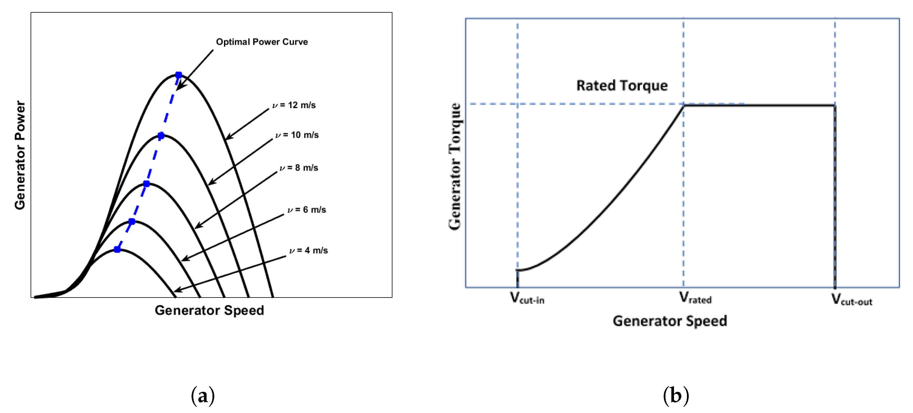
which requires maintaining $\lambda$ at its optimum value ${\lambda }_{opt}$ and the pitch angle at $\beta =0$. Figure 1 shows a typical wind turbine characteristics with the optimal power extraction $P_{opt}$. As the wind speed varies, the controller plays the role of ensuring that the wind turbine follows the optimal power curve in Figure 1a.

A wind turbine converts the mechanical power of the wind rotating the blades of the turbine into electrical power. In this paper, the one-mass derive train model is considered in which the total inertia $H_t$ is the sum of the turbine rotor and generator inertias. The dynamics of this model can be formulated as the differential equation:

$$2H_t\frac{d{\omega }_r}{dt}=T_m-T_e$$

(6)

where $T_m$ is the mechanical torque and $T_e$ is the electromechanical torques.

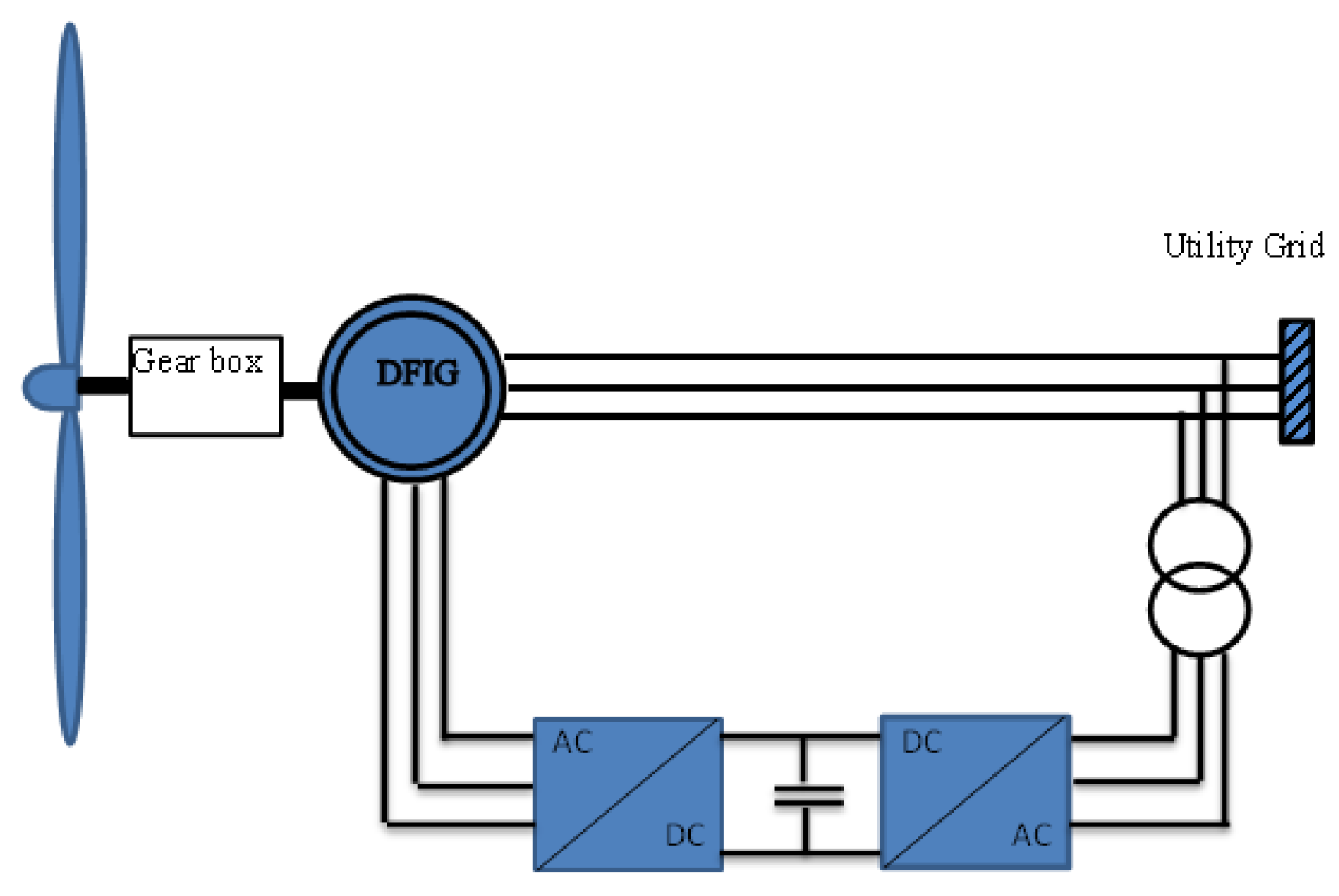
A typical configuration of a utility grid involving a DFIG is shown in Figure 2. For a simplified mathematical model, all equations of the induction generator are derived using the direct-quadrature (d-q) transformation. The stator and rotor voltage equations in d-q synchronous reference frame are given, respectively by:

$$\left[\begin{array}{c}{v}_{ds}\\ v_{qs}\end{array}\right]=-R_s\left[\begin{array}{c}{i}_{ds}\\ i_{qs}\end{array}\right]+{\omega }_s\left[\begin{array}{c}-{\psi }_{qs}\\ {\psi }_{ds}\end{array}\right]+\frac{1}{{\omega }_b}\frac{d}{dt}\left[\begin{array}{c}{\psi }_{ds}\\ {\psi }_{qs}\end{array}\right]$$

(7)

$$\left[\begin{array}{c}{v}_{dr}\\ v_{qr}\end{array}\right]=R_r\left[\begin{array}{c}{i}_{dr}\\ i_{qr}\end{array}\right]+s{\omega }_s\left[\begin{array}{c}-{\psi }_{qr}\\ {\psi }_{dr}\end{array}\right]+\frac{1}{{\omega }_b}\frac{d}{dt}\left[\begin{array}{c}{\psi }_{dr}\\ {\psi }_{qr}\end{array}\right]$$

(8)

where the subscripts s and r denote the stator and rotor quantities while subscripts q and d denote the components aligned with the q-axis and d-axis reference frames, respectively. In (7) and (8), $R_s$ and $R_r$ are the stator and rotor resistances, respectively, and ${\omega }_s$ and ${\omega }_b$ are synchronous and base angular frequencies, respectively. s is defined as the slip of the generator and given by $s=({\omega }_s-{\omega }_r)/{\omega }_s$. The corresponding magnetic flux equations are given by:

$$\begin{array}{c}\hfill \begin{array}{cc}\hfill {\psi }_{ds}& =L_s{i}_{ds}+L_m{i}_{dr}\hfill \\ \hfill {\psi }_{qs}& =L_s{i}_{qs}+L_m{i}_{qr}\hfill \\ \hfill {\psi }_{dr}& =L_r{i}_{dr}+L_m{i}_{ds}\hfill \\ \hfill {\psi }_{qr}& =L_r{i}_{qr}+L_m{i}_{qs}\hfill \end{array}\end{array}$$

(9)

where $L_s$, $L_r$, and $L_m$ are stator, rotor, and self magnetizing reactances, respectively. $L_s$ and $L_r$ are defined by the following equations:

$$\begin{array}{c}\hfill \begin{array}{cc}\hfill L_s& =L_{ls}+L_m\hfill \\ \hfill L_r& =L_{lr}+L_m\hfill \end{array}\end{array}$$

(10)

In [15,16] a synchronous reference frame was considered to derive the mathematical model. The following assumptions were imposed: (a) The stator current is assumed to be negative when flowing toward the machine; (b) q-axis is ${90}^{\circ }$ ahead of the d-axis with respect to the direction of rotation. In this paper, the current model of a single-cage DFIG wind turbine reported in [15,16] is considered. The general linearized state-space current model is given by:

$$\begin{array}{c}\hfill \begin{array}{cc}\hfill \dot{x}\left(t\right)& =Ax\left(t\right)+Bu\left(t\right)\hfill \\ \hfill y\left(t\right)& =Cx\left(t\right)+Du\left(t\right)\hfill \end{array}\end{array}$$

(11)

where $A,B,C,$ and D represent the system state, input, output, and feed forward matrices, respectively. The state-space variables, inputs and outputs of the fifth-order single-cage DFIG wind turbine can be described by the following vectors:

$$\dot{x}={\left[\begin{array}{cccc}{i}_{ds}& i_{qs}& i_{dr}& i_{qr}\end{array}\right]}^T$$

(12)

$$u={\left[\begin{array}{cccc}{v}_{ds}& v_{qs}& v_{dr}& v_{qr}\end{array}\right]}^T,y={\left[\begin{array}{cc}{i}_{dr}& i_{qr}\end{array}\right]}^T$$

(13)

where the state variables x are the rotor and stator currents, the control signals u are the input voltages and the outputs of the system y are the rotor currents in the d-axis and q-axis, respectively. In terms of state variables, the electromechanical torque can be formulated as:

$$T_e=L_m(i_{dr}{i}_{qs}-i_{qr}{i}_{ds})$$

(14)

using (6) and (14) we get

$${\dot{\omega }}_m=\frac{T_m}{2H_t}+\frac{L_m}{2H_t}(i_{qr}{i}_{ds}-i_{dr}{i}_{qs})$$

(15)

The state-space model of the fifth-order single-cage DFIG wind turbine is obtained by integrating Equations (12)–(15). The new state variables, control signal and outputs are given as follows:

$$\dot{x}={\left[\begin{array}{ccccc}{i}_{ds}& i_{qs}& i_{dr}& i_{qr}& {\omega }_m\end{array}\right]}^T$$

(16)

$$u={\left[\begin{array}{ccccc}{v}_{ds}& v_{qs}& v_{dr}& v_{qr}& T_m\end{array}\right]}^T,y={\left[\begin{array}{cc}{i}_{dr}& i_{qr}\end{array}\right]}^T$$

(17)

The linearized system, control and output matrices A, B, and C, evaluated at the system’s operating points, are characterized by [10,15,16]:

$$\begin{array}{ccc}\hfill A=K_G·& \left[\begin{array}{ccccc}-R_s{L}_r& {\alpha }_1{\omega }_s& -R_r{L}_m& -{\beta }_r{\omega }_s& a_{15}\\ -{\alpha }_1{\omega }_s& -R_s{L}_r& -{\beta }_r{\omega }_s& -R_r{L}_m& a_{25}\\ -R_s{L}_m& {\beta }_s{\omega }_s& -R_r{L}_s& -{\alpha }_2{\omega }_s& a_{35}\\ -{\beta }_s{\omega }_s& -R_s{L}_m& {\alpha }_2{\omega }_s& -R_r{L}_s& a_{45}\\ K_w{i}_{qr}& -K_w{i}_{dr}& -K_w{i}_{qs}& K_w{i}_{ds}& 0\end{array}\right],\hspace{1em}\hfill & B=K_G·\left[\begin{array}{ccccc}-L_r& 0& L_m& 0& 0\\ 0& -L_r& 0& L_m& 0\\ -L_m& 0& L_s& 0& 0\\ 0& -L_m& 0& L_s& 0\\ 0& 0& 0& 0& \frac{1}{2H_t}\end{array}\right],\hfill \\ \hfill C=& \left[\begin{array}{ccccc}0& 0& 1& 0& 0\\ 0& 0& 0& 1& 0\end{array}\right],D=\left[\begin{array}{ccccc}0& 0& 0& 0& 0\\ 0& 0& 0& 0& 0\end{array}\right]\hfill & \hfill \end{array}$$

(18)

where ${\alpha }_1=L_s{L}_r-s{L}_m^2$, ${\alpha }_2=L_m^2-s{L}_s{L}_r$, ${\beta }_s=L_m{L}_s(1-s)$, ${\beta }_r=L_m{L}_r(1-s)$, $\sigma =1-L_m^2/L_r{L}_s$, $K_G={\omega }_b{\left(L_s{L}_r\sigma \right)}^{-1}$, $K_w=L_m{\left(2H_t{K}_G\right)}^{-1}$, $a_{15}=L_m(L_m{i}_{qs}-L_r{i}_{qr})$, $a_{25}=L_m(-L_m{i}_{ds}+L_r{i}_{dr})$, $a_{35}=L_s(L_m{i}_{qs}-L_r{i}_{qr})$, $a_{45}=L_s(-L_m{i}_{ds}+L_r{i}_{dr})$.

Appendix A.1, Appendix A.2 and Appendix A.3 lists the parameters of the system and the DFIG, in addition to the operating points employed in the linearization procedure.

3. Exact Decomposition of the Algebraic Riccati Equation

Consider the linear singularly perturbed control system:

$$\begin{array}{c}\hfill \begin{array}{cc}\hfill {\dot{x}}_1\left(t\right)& =A_1{x}_1\left(t\right)+A_2{x}_2\left(t\right)+B_{1}u\left(t\right)\hfill \\ \hfill ϵ{\dot{x}}_2\left(t\right)& =A_3{x}_1\left(t\right)+A_4{x}_2\left(t\right)+B_{2}u\left(t\right)\hfill \end{array}\end{array}$$

(19)

where $x_i\left(t\right)\in {\Re }^n$, $i=1,2$, $u\left(t\right)\in {\Re }^m$ are the state variables and control variables, respectively. $ϵ$ is a small positive singular perturbation parameter that indicates system separation into slow and fast time scales. We assume that the singularly perturbed system (19) has the standard singular perturbation form [1]. Hence, the fast subsystem matrix $A_4$ is nonsingular, which is a standard assumption in the singular perturbation theory [1]. The corresponding linear-quadratic optimal control problem of (19) is defined by:

$$\begin{array}{c}\hfill \begin{array}{cc}\hfill {\dot{x}}_1\left(t\right)& =A_1{x}_1\left(t\right)+A_2{x}_2\left(t\right)+B_{1}u\left(t\right),x_1\left(0\right)=x_{10}\hfill \\ \hfill ϵ{\dot{x}}_2\left(t\right)& =A_3{x}_1\left(t\right)+A_4{x}_2\left(t\right)+B_{2}u\left(t\right),x_2\left(0\right)=x_{20}\hfill \end{array}\end{array}$$

(20)

where the control vector $u\in {\Re }^m$, has to be chosen such that the following performance criterion, J, is minimized

$$\underset{u}{min}J=\underset{u}{min}\frac{1}{2}{\int }_0^{\infty }\left\{{\left[\begin{array}{c}{x}_1\left(t\right)\\ x_2\left(t\right)\end{array}\right]}^{T}Q\left[\begin{array}{c}{x}_1\left(t\right)\\ x_2\left(t\right)\end{array}\right]+u^T\left(t\right)Ru\left(t\right)\right\}dt$$

(21)

where $R>0$ and $Q\ge 0$ are the weighting matrices. The optimizing performance criterion (21) of the closed-loop optimal control problem, subject to the singularly perturbed system differential Equation (20), has the solution

$$u\left(t\right)=-R^{-1}{B}^T{P}_{r}x\left(t\right)=-F_1{x}_1-F_2{x}_2$$

(22)

where $P_r$ is the positive semidefinite solution of the regulator algebraic Riccati equation given by [17]

$$0=P_{r}A+A^T{P}_r+Q-P_{r}Z{P}_r,$$

(23)

with

$$A=\left[\begin{array}{cc}{A}_1& A_2\\ \frac{1}{ϵ}{A}_3& \frac{1}{ϵ}{A}_4\end{array}\right],Q=\left[\begin{array}{cc}{Q}_1& Q_2\\ Q_2^T& Q_3\end{array}\right]$$

(24)

$$B=\left[\begin{array}{c}{B}_1\\ \frac{1}{ϵ}{B}_2\end{array}\right],P_r=\left[\begin{array}{cc}{P}_{1r}& ϵP_{2r}\\ ϵP_{2r}^T& ϵP_{3r}\end{array}\right],Z=B_1{R}^{-1}{B}_2^T$$

The optimal regulator gains $F_1$ and $F_2$ are given by

$$\begin{array}{c}\hfill \begin{array}{c}\hfill F_1=R^{-1}(B_1^T{P}_{1r}+B_2^T{P}_{2r}^T)\\ \hfill F_2=R^{-1}(ϵB_1^T{P}_{2r}+B_2^T{P}_{3r})\end{array}\end{array}$$

(25)

The solution of the algebraic Riccati Equation (23) will be found in term of solutions of the reduced-order, pure-slow and pure-fast algebraic Riccati equation. For this purpose, a nonsingular transformation $\mathit{T}$ [18,19] is applied for the state-costate equations such that they become completely decoupled as independent slow and fast subsystems in the form

$$\begin{array}{c}\hfill \begin{array}{cc}\hfill {\dot{\zeta }}_s\left(t\right)& =(a_1+a_2{P}_{rs}){\zeta }_s\left(t\right)\hfill \\ \hfill ϵ{\dot{\zeta }}_f\left(t\right)& =(b_1+b_2{P}_{rf}){\zeta }_f\left(t\right)\hfill \end{array}\end{array}$$

(26)

where $P_{rs}$ and $P_{rf}$ are the unique solutions of the exact pure-slow and exact pure-fast completely decoupled algebraic regulator Riccati equations

$$\begin{array}{c}\hfill \begin{array}{cc}\hfill 0& =P_{rs}{a}_1-a_4{P}_{rs}-a_3+P_{rs}{a}_2{P}_{rs}\hfill \\ \hfill 0& =P_{rf}{b}_1-b_4{P}_{rf}-b_3+P_{rf}{b}_2{P}_{rf}\hfill \end{array}\end{array}$$

(27)

Matrices $a_i,b_i,i=1,2,3,4$, can be found in [18,19]. The nonsingular transformation $\mathit{T}$ is given by:

$$\mathit{T}=({\mathsf{\Pi }}_1+{\mathsf{\Pi }}_2{P}_r)$$

(28)

The slow and fast subsystems in the new coordinate are related by:

$$\left[\begin{array}{c}{\zeta }_s\left(t\right)\\ {\zeta }_f\left(t\right)\end{array}\right]=\mathit{T}\left[\begin{array}{c}{x}_1\left(t\right)\\ x_2\left(t\right)\end{array}\right]$$

(29)

Even more, the global solution $P_r$ can be obtained from the reduced-order exact pure-slow and pure-fast algebraic Riccati equations, that is

$$P_{rsf}=\left({\mathsf{\Omega }}_3+{\mathsf{\Omega }}_4\left[\begin{array}{cc}{P}_{rs}& 0\\ 0& P_{rf}\end{array}\right]\right){\left({\mathsf{\Omega }}_1+{\mathsf{\Omega }}_2\left[\begin{array}{cc}{P}_{rs}& 0\\ 0& P_{rf}\end{array}\right]\right)}^{-1}$$

(30)

Known matrices ${\mathsf{\Omega }}_i$, $i=1,2,3,4$, and ${\mathsf{\Pi }}_1$, ${\mathsf{\Pi }}_2$ are given in terms of solutions of the Chang decoupling equations [18,19].

3.1. Optimal Performance Invariance to Similarity Transformation

It has been shown in [20] that similarity transformation preserves the optimal performance criteria for the linear quadratic regulator LQR, such that its optimal values in the two coordinate systems are equivalent. This results can be derived briefly as follows:

The similarity transformation for the linear quadratic optimal control problem can be derived as follows:

$$\begin{array}{c}\hfill \left.\begin{array}{c}\hfill \dot{x}=Ax+Bu,,\\ \hfill x\left(0\right)=x_0,\\ \hfill J=\frac{1}{2}{\int }_0^{\infty }\left(x^{T}Qx+u^{T}Ru\right)dt\\ \hfill J_{opt}=\frac{1}{2}{x}_{0}P{x}_0\\ \hfill A^{T}P+PA+Q-PB{R}^{-1}{B}^{T}P=0\end{array}\right\}\underrightarrow{\overline{x}=Tx}\left\{\begin{array}{c}\hfill \dot{\overline{x}}=\overline{A}\overline{x}+\overline{B}u,\\ \hfill {\overline{x}}_0=T{x}_0,\\ \hfill \overline{J}=\frac{1}{2}{\int }_0^{\infty }\left({\overline{x}}^T\overline{Q}\overline{x}+u^{T}Ru\right)dt\\ \hfill {\overline{J}}_{opt}=\frac{1}{2}\overline{x_0}\overline{P}\overline{x_0}\\ \hfill \overline{A}\overline{P}+\overline{P}\overline{A}+\overline{Q}-\overline{P}\overline{B}{R}^{-1}{\overline{B}}^T\overline{P}=0\end{array}\right.\end{array}$$

Derivations:

$$\dot{\overline{x}}=T\dot{x}=TAx+TBu=TA{T}^{-1}\overline{x}+TBu$$

(31)

$$\overline{A}=TA{T}^{-1},\overline{B}=TB,\overline{Q}=T^{-T}QT$$

(32)

$$\overline{A}\overline{P}+\overline{P}\overline{A}+\overline{Q}-\overline{P}\overline{B}{R}^{-1}{\overline{B}}^T\overline{P}=0$$

(33)

$$T^{-T}{A}^T{T}^T\overline{P}+\overline{P}TA{T}^{-1}+\overline{Q}-\overline{P}TB{R}^{-1}{B}^T{T}^T\overline{P}=0$$

(34)

Multiplying by $T^T$ from the left and by T from the right we get

$$A^T{T}^T\overline{P}T+T^T\overline{P}TA+T^T\overline{Q}T-T^T\overline{P}TB{R}^{-1}{B}^T{T}^T\overline{P}P=0$$

(35)

define $P=T^T\overline{P}T$, $\overline{P}=T^{-T}P{T}^{-1}$, then

$$A^{T}P+PA+Q-PB{R}^{-1}{B}^{T}P=0$$

(36)

$${\overline{J}}_{opt}=\frac{1}{2}\overline{x_0}\overline{P}\overline{x_0}=\frac{1}{2}{x}_0^T{T}^T{T}^{-T}P{T}^{-1}T{x}_0=\frac{1}{2}{x}_0^{T}P{x}_0$$

(37)

$${\overline{J}}_{opt}=J_{opt}$$

(38)

3.2. Slow and Fast Decomposition of the Optimal Performance Criteria

In this section, we calculate the minimized optimal performance $J_{opt}$ for the slow and fast subsystems of the LQR problem. As stated in the previous section, using the nonsingular transformation defined in (28) does not change the value of the optimal performance. Therefore, by adding the slow and fast performance indices, we get the total optimal performance $J_{opt}$ obtained in the original coordinates. The quadratic performance criterion to be minimized, calculated in the new coordinates, is given by:

$$J=\frac{1}{2}{\int }_0^{\infty }\left\{x^{T}Qx+u^{T}Ru\right\}dt=\frac{1}{2}{\int }_0^{\infty }\left\{x^T\left(t\right)(Q+PSP)x\left(t\right)\right\}dt$$

(39)

$$x\left(t\right)={({\mathsf{\Pi }}_1+{\mathsf{\Pi }}_{2}P)}^{-1}\left[\begin{array}{c}{\eta }_1\left(t\right)\\ {\zeta }_1\left(t\right)\end{array}\right]={\mathit{T}}^{-1}\left[\begin{array}{c}{\eta }_1\left(t\right)\\ {\zeta }_1\left(t\right)\end{array}\right]$$

(40)

$$J=\frac{1}{2}{\int }_0^{\infty }\left[\begin{array}{c}{\eta }_1\left(t\right)\\ {\zeta }_1\left(t\right)\end{array}\right]T^{-1}(Q+PSP)T\left[\begin{array}{c}{\eta }_1\left(t\right)\\ {\zeta }_1\left(t\right)\end{array}\right]=\frac{1}{2}{\int }_0^{\infty }\left[\begin{array}{c}{\eta }_1\left(t\right)\\ {\zeta }_1\left(t\right)\end{array}\right]\left[\begin{array}{cc}{Q}_1& Q_2\\ Q_2^T& Q_3\end{array}\right]\left[\begin{array}{c}{\eta }_1\left(t\right)\\ {\zeta }_1\left(t\right)\end{array}\right]dt$$

(41)

$$\begin{array}{c}\hfill \begin{array}{cc}\hfill {\dot{\zeta }}_1\left(t\right)& =(a_1+a_2{P}_s){\zeta }_1\left(t\right)\hfill \\ \hfill ϵ{\dot{\zeta }}_2\left(t\right)& =(b_1+b_2{P}_f){\zeta }_2\left(t\right)\hfill \end{array}\end{array}$$

(42)

$$J=\frac{1}{2}{\left[\begin{array}{c}{\eta }_1\left(0\right)\\ {\zeta }_1\left(0\right)\end{array}\right]}^{T}V\left[\begin{array}{c}{\eta }_1\left(0\right)\\ {\zeta }_1\left(0\right)\end{array}\right],A^{T}V+VA+\theta =0$$

(43)

$$J=\frac{1}{2}\left[\begin{array}{cc}{\eta }_1^T\left(0\right)& {\zeta }_1^T\left(0\right)\end{array}\right]\left[\begin{array}{cc}{v}_1& ϵv_2\\ ϵv_2^T& ϵv_3\end{array}\right]\left[\begin{array}{c}{\eta }_1\left(0\right)\\ {\zeta }_1\left(0\right)\end{array}\right]$$

(44)

$$J=\frac{1}{2}[{\eta }_1^T\left(0\right)v_1+ϵ{\zeta }_1^T\left(0\right)v_2^T⋮ϵ{\eta }_1^T\left(0\right)v_2+ϵ{\zeta }_1^T\left(0\right)v_3]\left[\begin{array}{c}{\eta }_1\left(0\right)\\ {\zeta }_1\left(0\right)\end{array}\right]$$

(45)

$$J=\frac{1}{2}{\eta }_1^T\left(0\right)v_1{\eta }_1\left(0\right)+\frac{1}{2}ϵ{\zeta }_1^T\left(0\right)v_2^T{\eta }_1\left(0\right)+\frac{1}{2}ϵ{\eta }_1^T\left(0\right)v_2{\zeta }_1\left(0\right)+\frac{1}{2}ϵ{\zeta }_1^T\left(0\right)v_3{\zeta }_1\left(0\right)$$

(46)

$$J=\underset{J_{s-opt}}{\underbrace{\frac{1}{2}{\eta }_1^T\left(0\right)v_1{\eta }_1\left(0\right)}}+\underset{J_{sf-opt}}{\underbrace{ϵ{\eta }_1^T\left(0\right)v_2{\zeta }_1\left(0\right)}}+\underset{J_{f-opt}}{\underbrace{\frac{1}{2}ϵ{\zeta }_1^T\left(0\right)v_3{\zeta }_1\left(0\right)}}$$

(47)

$$J_{opt}=J_{s-opt}+J_{sf-opt}+J_{f-opt}$$

(48)

$$J_{s-opt}=\frac{1}{2}{\eta }_1^T\left(0\right)v_1{\eta }_1\left(0\right)=\frac{1}{2}tr\left\{v_1{\eta }_1\left(0\right){\eta }_1^T\left(0\right)\right\}$$

(49)

$$J_{f-opt}=\frac{ϵ}{2}{\zeta }_1^T\left(0\right)v_3{\zeta }_1\left(0\right)=\frac{ϵ}{2}tr\left\{v_3{\zeta }_1\left(0\right){\zeta }_1^T\left(0\right)\right\}$$

(50)

$$J_{sf-opt}=ϵ{\eta }_1^T\left(0\right)v_2{\zeta }_1\left(0\right)=ϵtr\left\{v_2{\zeta }_1\left(0\right){\eta }_1^T\left(0\right)\right\}$$

(51)

Formula (47) constitutes an exact decomposition for the optimal performance criterion into slow and fast components. It can be concluded from (47) that the contribution the slow subsystem makes to the performance criterion is $O\left(1\right)$, whereas that the fast subsystem makes is only $O\left(ϵ\right)$. Note also that $J_{sf-opt}$ can be negative since $v_2$ is generally not a square matrix, and in the case it is, it would still be indefinite.

4. Kalman Filtering Time Scale Analysis

In this section, an optimal Kalman filter is designed to estimate the state variables of the wind energy systems with DFIG. Using the duality property between the optimal filter and regulator, the same decomposition method presented in previous section can be applied here so that the optimal Kalman filter is completely decoupled into the pure-slow and pure-fast local filters both driven by the system measurements [17]. Consider the linear continuous-time invariant singularly perturbed stochastic system

$$\begin{array}{c}\hfill \begin{array}{cc}\hfill {\dot{x}}_1\left(t\right)& =A_1{x}_1\left(t\right)+A_2{x}_2\left(t\right)+B_{1}u\left(t\right)+G_1{w}_1\left(t\right),E\left\{x_1\left(0\right)\right\}=x_{10}\hfill \\ \hfill ϵ{\dot{x}}_2\left(t\right)& =A_3{x}_1\left(t\right)+A_4{x}_2\left(t\right)+B_{2}u\left(t\right)+G_2{w}_1\left(t\right),E\left\{x_2\left(0\right)\right\}=x_{20}\hfill \\ \hfill y\left(t\right)& =C_1{x}_1\left(t\right)+C_2{x}_2\left(t\right)+w_2\left(t\right)\hfill \end{array}\end{array}$$

(52)

with the performance criterion

$$J=\underset{t_f\to \infty }{lim}\frac{1}{t_f}\left\{{\int }_0^t\left[z^T\left(t\right)z\left(t\right)+u^T\left(t\right)Ru\left(t\right)\right]dt\right\}, R>0$$

(53)

where $x_1\left(t\right)\in {\Re }_1^n$, and $x_2\left(t\right)\in {\Re }_2^n$, are slow and fast state variables, respectively. $u\left(t\right)\in {\Re }^m$ is the control input, $y\left(t\right)\in {\Re }^p$ are system measurements. $w_1\left(t\right)\in {\Re }^r$ and $w_2\left(t\right)\in {\Re }^p$ are zero-mean stationary, white Gaussian noise stochastic process with intensities $W_1>0$ and $W_2>0$, respectively. $z\left(t\right)\in {\Re }^s$, is the controlled system output given by:

$$z\left(t\right)=D_1{x}_1\left(t\right)+D_2{x}_2\left(t\right)$$

(54)

All matrices are of appropriate dimensions and assumed to be constant. The optimal control law for (52) with the performance criterion (53) is given by:

$$u_{opt}\left(t\right)=-F_1{\widehat{x}}_1\left(t\right)-F_2{\widehat{x}}_2\left(t\right)$$

(55)

where ${\widehat{x}}_1\left(t\right)$ and ${\widehat{x}}_2\left(t\right)$ are the optimal estimates of the state vectors $x_1\left(t\right)$ and $x_1\left(t\right)$ obtained from the Kalman filter

$$\begin{array}{c}\hfill \begin{array}{cc}\hfill {\dot{\widehat{x}}}_1\left(t\right)& =A_1{\widehat{x}}_1\left(t\right)+A_2{\widehat{x}}_2\left(t\right)+B_{1}u\left(t\right)+K_{1}v\left(t\right)\hfill \\ \hfill ϵ{\dot{\widehat{x}}}_2\left(t\right)& =A_3{\widehat{x}}_1\left(t\right)+A_4{\widehat{x}}_2\left(t\right)+B_{2}u\left(t\right)+K_{2}v\left(t\right)\hfill \\ \hfill v\left(t\right)& =y\left(t\right)-C_1{\widehat{x}}_1\left(t\right)-C_2{\widehat{x}}_2\left(t\right)\hfill \end{array}\end{array}$$

(56)

The optimal global Kalman filter (56) can be put in the form in which the filter is driven by the system measurements and optimal control inputs, that is

$$\begin{array}{c}\hfill \begin{array}{cc}\hfill {\dot{\widehat{x}}}_1\left(t\right)& =(A_1-K_1{C}_1){\widehat{x}}_1\left(t\right)+(A_2-K_1{C}_2){\widehat{x}}_2\left(t\right)+B_{1}u\left(t\right)+K_{1}y\left(t\right)\hfill \\ \hfill ϵ{\dot{\widehat{x}}}_2\left(t\right)& =(A_3-K_2{C}_1){\widehat{x}}_1\left(t\right)+(A_4-K_2{C}_2){\widehat{x}}_2\left(t\right)+B_{2}u\left(t\right)+K_{2}y\left(t\right)\hfill \end{array}\end{array}$$

(57)

where the optimal filter gains $K_1$ and $K_2$ are obtained from

$$\begin{array}{c}\hfill \begin{array}{cc}\hfill K_1& =(P_{1F}{C}_1^T+P_{2F}{C}_2^T)W_2^{-1}\hfill \\ \hfill K_2& =(ϵP_{2F}^T{C}_1^T+P_{3F}{C}_2^T)W_2^{-1}\hfill \end{array}\end{array}$$

(58)

matrices $P_{1F}$, $P_{2F}$ and $P_{3F}$ define the positive semidefinite stabilizing solution of the filter algebraic Riccati equation

$$A{P}_F+P_F{A}^T-P_{F}S{P}_F+G{W}_1{G}^T=0$$

(59)

where

$$A=\left[\begin{array}{cc}{A}_1& A_2\\ \frac{1}{ϵ}{A}_3& \frac{1}{ϵ}{A}_3\end{array}\right],G=\left[\begin{array}{c}{G}_1\\ \frac{1}{ϵ}{G}_2\end{array}\right],S=C^T{W}_2^{-1}C,P_F=\left[\begin{array}{cc}{P}_{1F}& P_{2F}\\ P_{2F}^T& \frac{1}{ϵ}{P}_{3F}\end{array}\right]$$

(60)

Using duality, the following matrices have to be formed (see [18,19])

$$\begin{array}{c}\hfill \begin{array}{cc}\hfill & T_{1F}=\left[\begin{array}{cc}{A}_1^T& -C_1^T{W}_2^{-1}{C}_1\\ -G_1{W}_1{G}_1^T& -A_1\end{array}\right],T_{2F}=\left[\begin{array}{cc}{A}_3^T& -C_1^T{W}_2^{-1}{C}_2\\ -G_1{W}_1{G}_2^T& -A_2\end{array}\right],\hfill \\ \hfill & T_{3F}=\left[\begin{array}{cc}{A}_2^T& -C_2^T{W}_2^{-1}{C}_1\\ -G_2{W}_1{G}_1^T& -A_3\end{array}\right],T_{4F}=\left[\begin{array}{cc}{A}_4^T& -C_2^T{W}_2^{-1}{C}_2\\ -G_2{W}_1{G}_2^T& -A_4\end{array}\right],\hfill \end{array}\end{array}$$

(61)

The partitions and scaling have to be used here, $x^T\left(t\right)=\left[x_1^T\left(t\right)ϵx_2^T\left(t\right)\right]$ and $p^T\left(t\right)=\left[p_1^T\left(t\right)p_2^T\left(t\right)\right]$. Since matrices $T_{1F}$, $T_{2F}$, $T_{3F}$, and $T_{4F}$ correspond to the system matrices of a singularly perturbed linear system, the slow-fast decomposition is achieved by using the Chang decoupling equations

$$\begin{array}{c}\hfill \begin{array}{cc}\hfill & T_{4F}M-T_{3F}-ϵM(T_{1F}-T_{2F}M)=0\hfill \\ \hfill -N(T_{4F}& +ϵM{T}_{2F})+T_{2F}+ϵ(T_{1F}-T_{2F}M)N=0\hfill \end{array}\end{array}$$

(62)

Using the following permutation matrices,

$$E_{1F}=\left[\begin{array}{cccc}{I}_{n_1}& 0& 0& 0\\ 0& 0& I_{n_1}& 0\\ 0& \frac{1}{ϵ}{I}_{n_2}& 0& 0\\ 0& 0& 0& I_{n_2}\end{array}\right],E_{2F}=\left[\begin{array}{cccc}{I}_{n_1}& 0& 0& 0\\ 0& 0& I_{n_1}& 0\\ 0& I_{n_2}& 0& 0\\ 0& 0& 0& I_{n_2}\end{array}\right]$$

(63)

we can define

$${\mathsf{\Pi }}_F=\left[\begin{array}{cc}{\mathsf{\Pi }}_{1F}& {\mathsf{\Pi }}_{2F}\\ {\mathsf{\Pi }}_{3F}& {\mathsf{\Pi }}_{4F}\end{array}\right]=E_{2F}^T\left[\begin{array}{cc}{I}_{2n_1}-ϵNM& -ϵN\\ M& I_{2n_2}\end{array}\right]E_{1F}$$

(64)

Then, the desired transformation is given by:

$${\mathit{T}}_{\mathbf{2}}=({\mathsf{\Pi }}_{1F}+{\mathsf{\Pi }}_{2F}{P}_F)$$

(65)

where $P_F$ is the solution of the ARE (59). M and N are the solution of the Chang decoupling algebraic Equations (62). The transformation ${\mathit{T}}_{\mathbf{2}}$ is applied to the filter variables as:

$$\left[\begin{array}{c}\widehat{{\eta }_s}\left(t\right)\\ \widehat{{\eta }_f}\left(t\right)\end{array}\right]={\mathit{T}}_{\mathbf{2}}^{-\mathit{T}}\left[\begin{array}{c}{\widehat{x}}_1\left(t\right)\\ {\widehat{x}}_2\left(t\right)\end{array}\right]$$

(66)

Kalman Filter Under Similarity Transformation

To determine the gain of Kalman filter in the new coordinates under a similarity transformation, the same strategy used in Section 3.1 is applied here

$$\begin{array}{c}\hfill \begin{array}{cc}\hfill \dot{x}\left(t\right)& =Ax\left(t\right)+G{w}_1\left(t\right),x\left(0\right)=x_0\hfill \\ \hfill y\left(t\right)& =Cx\left(t\right)+w_2\left(t\right)\hfill \end{array}\end{array}$$

(67)

$$\dot{\widehat{x}}=(A-KC)\widehat{x}+Ky,K=P_F{C}^T{W}_2,E\left\{\widehat{x}\left(0\right)\right\}=x_0$$

(68)

$$A{P}_F+P_F{A}^T+G{W}_1{G}^T-P_{F}C{W}_2^{-1}{C}^T{P}_F=0$$

(69)

$$\begin{array}{c}\hfill \begin{array}{cc}\hfill \dot{\overline{x}}\left(t\right)& =\overline{A}\overline{x}\left(t\right)+\overline{G}{w}_1\left(t\right),x\left(0\right)=x_0\hfill \\ \hfill y\left(t\right)& =\overline{C}\overline{x}\left(t\right)+w_2\left(t\right),\hfill \end{array}\end{array}$$

(70)

$\overline{G}=TG,\overline{C}=C{T}^{-1},$ in the new coordinates $\overline{K}=\overline{P_F}{\overline{C}}^T{W}_2$ and

$$\overline{A}\overline{P_F}+\overline{P_F}{\overline{A}}^T+\overline{G}{W}_1{\overline{G}}^T-\overline{P_F}{\overline{C}}^T{W}_2^{-1}\overline{C}\overline{P_F}=0$$

(71)

$$TA{T}^{-1}\overline{P_F}+\overline{P_F}{T}^{-T}{A}^T{T}^T+TG{W}_1{G}^T{T}^T-\overline{P_F}{T}^{-T}{C}^T{W}_2^{-1}C{T}^{-1}\overline{P_F}=0$$

(72)

Multiplying by $T^{-1}$ from the left and by $T^{-T}$ from the right we get:

$$A{T}^{-1}\overline{P_F}{T}^{-T}+T^{-1}\overline{P_F}{T}^{-T}{A}^T+G{W}_1{G}^T-T^{-1}\overline{P_F}{T}^{-T}{C}^T{W}_2^{-1}C{T}^{-1}\overline{P_F}{T}^{-T}=0$$

(73)

$$\overline{K}=T{P}_F{T}^T{T}^{-T}{C}^T{W}_2=T{P}_F{C}^T{W}_2=TK$$

(74)

where $P_F=T^{-1}\overline{P_F}{T}^{-T}$, $\overline{P}=T{P}_F{T}^T$

5. Optimal Linear-Quadratic Gaussian Control

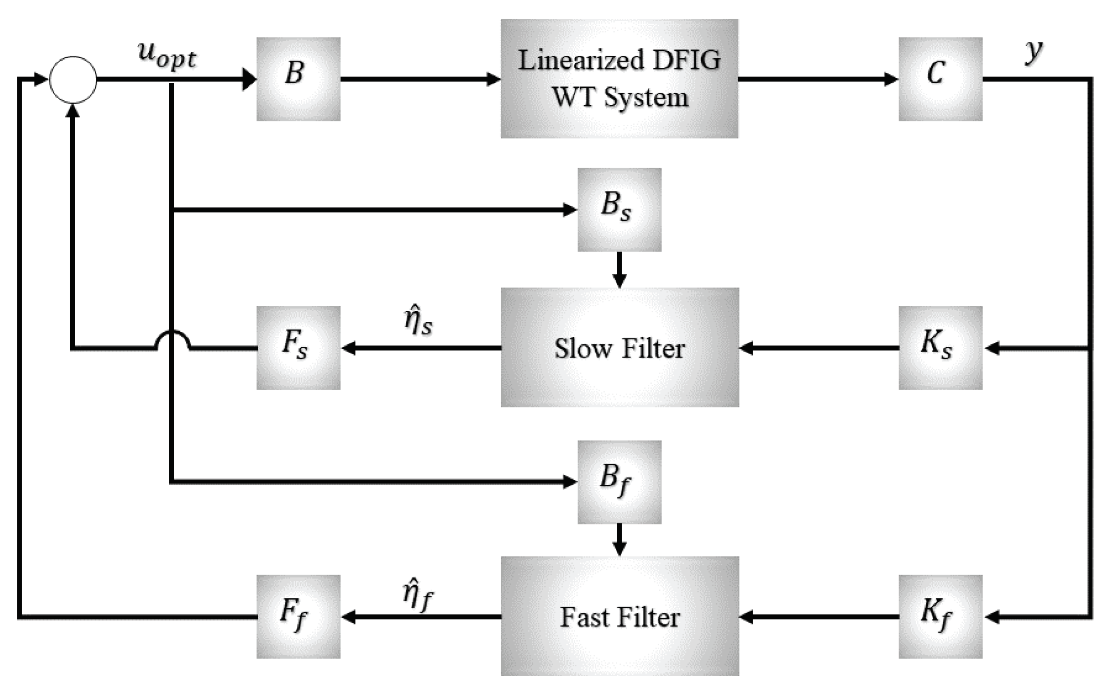
In order to obtain the solution of the linear-quadratic Gaussian LQG control problem of a singularly perturbed DFIG wind turbine system, it is necessary to obtain gain matrices of the the optimal LQR and Kalman filters. In this section, the results of Section 3 and Section 4 are utilized by solving the pure-slow and pure-fast, reduced-order AREs and by implementing the pure-slow and pure-fast, reduced-order Kalman filters. Using the separation principle for linear stochastic control, an optimal LQG controller can be designed for slow and fast subsystems independently, thus, achieving complete separation and parallelism in the design process. The structure of a LQG controller with a decoupled slow and fast subsystems of the LQR and Kalman filter is shown in Figure 3. The decoupled pure-slow and pure-fast local Kalman filters driven by system measurements and system control inputs are given by:

$$\begin{array}{c}\hfill \begin{array}{cc}\hfill {\dot{\widehat{\eta }}}_s\left(t\right)& ={(a_{1F}+a_{2F}{P}_{sF})}^T{\widehat{\eta }}_s\left(t\right)+B_{s}u\left(t\right)+K_{s}y\left(t\right)\hfill \\ \hfill ϵ{\dot{\widehat{\eta }}}_f\left(t\right)& ={(b_{1F}+b_{2F}{P}_{fF})}^T{\widehat{\eta }}_f\left(t\right)+B_{f}u\left(t\right)+K_{f}y\left(t\right)\hfill \end{array}\end{array}$$

(75)

where $P_{sF}$ and $P_{fF}$ are the solutions of the following AREs

$$\begin{array}{c}\hfill \begin{array}{c}\hfill 0=P_{sF}{a}_{1F}-a_{4F}{P}_{sF}-a_{3F}+P_{sF}{a}_{2F}{P}_{sF}\\ \hfill 0=P_{fF}{b}_{1F}-b_{4F}{P}_{fF}-b_{3F}+P_{fF}{b}_{2F}{P}_{fF}\end{array}\end{array}$$

(76)

The pure-slow and pure-fast filter gains, $K_s$, $K_f$ are defined by

$$\left[\begin{array}{c}{K}_s\\ \frac{1}{ϵ}{K}_f\end{array}\right]={\mathit{T}}_{\mathbf{2}}^{-\mathit{T}}\left[\begin{array}{c}{K}_1\\ \frac{1}{ϵ}{K}_2\end{array}\right]$$

(77)

and the remaining matrices are given by:

$$\begin{array}{c}\hfill \begin{array}{cc}\hfill \left[\begin{array}{cc}{a}_{1F}& a_{2F}\\ a_{3F}& a_{4F}\end{array}\right]=(T_{1F}& -T_{2F}M),\left[\begin{array}{cc}{b}_{1F}& b_{2F}\\ b_{3F}& b_{4F}\end{array}\right]=(T_{4F}+ϵM{T}_{2F})\hfill \end{array}\end{array}$$

(78)

In addition, the pure-slow and pure-fast system input matrices are

$$\left[\begin{array}{c}{B}_s\\ \frac{1}{ϵ}{B}_f\end{array}\right]={\mathit{T}}_{\mathbf{2}}^{-\mathit{T}}\left[\begin{array}{c}{B}_1\\ \frac{1}{ϵ}{B}_2\end{array}\right]$$

(79)

The feedback control in the new coordinates is given:

$$u_{opt}\left(t\right)=-F\widehat{x}\left(t\right)=-F{\mathit{T}}_{\mathbf{2}}^{-\mathit{T}}\left[\begin{array}{c}\widehat{{\eta }_s}\left(t\right)\\ \widehat{{\eta }_f}\left(t\right)\end{array}\right]=-\left[\begin{array}{cc}{F}_s& F_f\end{array}\right]\left[\begin{array}{c}\widehat{{\eta }_s}\left(t\right)\\ \widehat{{\eta }_f}\left(t\right)\end{array}\right]$$

(80)

where $F_s$ and $F_f$ are obtained from:

$$\left[\begin{array}{cc}{F}_s& F_f\end{array}\right]=F{\mathit{T}}_{\mathbf{2}}^T=R^{-1}{B}^{T}P{({\mathsf{\Pi }}_{1F}+{\mathsf{\Pi }}_{2F}{P}_F)}^T$$

(81)

5.1. LQG under Similarity Transformation

The optimal performance index $J_{opt}$ of the LQG follows from the known formula

$$\begin{array}{c}\hfill \begin{array}{cc}\hfill J_{opt}& =tr\left\{PK{W}_2{K}^T+P_F{D}^{T}D\right\}\hfill \\ \hfill & =tr\left\{PG{W}_1{G}^T+P_F{F}^{T}RF\right\}\hfill \end{array}\end{array}$$

(82)

Under the similarity transformation, the performance criteria can be derived as follows. Starting with the second line of (82)

$${\overline{J}}_{opt}=tr\left\{\overline{P}\overline{G}{W}_1{\overline{G}}^T+{\overline{P}}_F{\overline{F}}^{T}R\overline{F}\right\}$$

(83)

$${\overline{J}}_{opt}=tr\left\{T^{-T}P{T}^{-1}TG{W}_1{G}^T{T}^T+T{P}_F{T}^T{T}^{-T}{F}^{T}RF{T}^{-1}\right\}$$

(84)

where $P_F=T^{-1}\overline{P_F}{T}^{-T}$, $\overline{P}=T{P}_F{T}^T$, $F=\overline{F}T$

$${\overline{J}}_{opt}=tr\left\{T^{-T}\left(PG{W}_1{G}^T\right)T^T+T\left(P_F{F}^{T}RF\right)T^{-1}\right\}\ne J_{opt}$$

(85)

Similarly, for the first line in (82), we have

$$J_{opt}=tr\left\{PK{W}_2{K}^T+P_F{D}^{T}D\right\}$$

(86)

where $D^{T}D=Q$, $\overline{K}=TK$

$${\overline{J}}_{opt}=tr\left\{\overline{P}\overline{K}{W}_2{\overline{K}}^T+{\overline{P}}_F\overline{Q}\right\}$$

(87)

$${\overline{J}}_{opt}=tr\left\{T^{-T}P{T}^{-1}TK{W}_2{K}^T{T}^T+T{P}_F{T}^T{T}^{-T}Q{T}^{-1}\right\}$$

(88)

$${\overline{J}}_{opt}=tr\left\{T^{-T}\left(PK{W}_2{K}^T\right)T^T+T\left(P_{F}Q\right)T^{-1}\right\}\ne J_{opt}$$

(89)

Hence, the similarity transformation does not preserve the optimal performance criteria of the LQG.

5.2. LQG Slow Fast Optimal Performance Criteria

Based on the method proposed in [19], the optimal performance index for the slow and fast subsytems of the LQG controller can be obtained separately as follows:

$$J_{opt}=tr\left\{PK{W}_2{K}^T+P_F{D}^{T}D\right\}$$

(90)

where $D^{T}D=Q;Q=\left[\begin{array}{cc}{Q}_1& Q_2\\ Q_2^T& Q_3\end{array}\right]$

$$P=\left[\begin{array}{cc}{P}_1& ϵP_2\\ ϵP_2^T& ϵP_3\end{array}\right],K=\left[\begin{array}{c}{K}_1\\ \frac{1}{ϵ}{K}_2\end{array}\right],P_F=\left[\begin{array}{cc}{P}_{1F}& P_{2F}\\ P_{2F}^T& \frac{1}{ϵ}{P}_{3F}\end{array}\right]$$

(91)

$$J_{opt}=tr\left\{\left[\begin{array}{cc}{P}_1& ϵP_2\\ ϵP_2^T& ϵP_3\end{array}\right]\left[\begin{array}{c}{K}_1\\ \frac{1}{ϵ}{K}_2\end{array}\right]W_2\left[\begin{array}{cc}{K}_1^T& \frac{1}{ϵ}{K}_2^T\end{array}\right]+\left[\begin{array}{cc}{P}_{1F}& P_{2F}\\ P_{2F}^T& \frac{1}{ϵ}{P}_{3F}\end{array}\right]\left[\begin{array}{cc}{Q}_1& Q_2\\ Q_2^T& Q_3\end{array}\right]\right\}$$

(92)

$$J_{opt}=tr\{\left[\begin{array}{cc}{P}_1& ϵP_2\\ ϵP_2^T& ϵP_3\end{array}\right]\left[\begin{array}{cc}{K}_1{w}_2{K}_1^T& \frac{1}{ϵ}{K}_1{w}_2{K}_2^T\\ \frac{1}{ϵ}{K}_2{w}_2{K}_1^T& {\frac{1}{ϵ}}^2{K}_2{w}_2{K}_2^T\end{array}\right]+\left[\begin{array}{cc}{P}_{1F}{Q}_1+ϵP_{2F}{Q}_2^T& ϵP_{1F}{Q}_2+ϵP_{2F}{Q}_3\\ P_{2F}^T{Q}_1+P_{3F}{Q}_2^T& P_{2F}^T{Q}_2+P_{3F}{Q}_3\end{array}\right]$$

(93)

$$\begin{array}{c}\hfill \begin{array}{cc}\hfill J_{opt}=& tr\{\left[\begin{array}{cc}{P}_1{K}_1{W}_2{K}_1^T+P_2{K}_2{W}_2{K}_1^T& \frac{1}{ϵ}{P}_1{K}_1{W}_2{K}_2^T+\frac{1}{ϵ}{P}_2{K}_2{W}_2{K}_2^T\\ ϵP_2^T{K}_1{W}_2{K}_1^T+P_3{K}_2{W}_2{K}_1^T& P_2^T{K}_1{W}_2{K}_2^T+\frac{1}{ϵ}{P}_3{K}_2{W}_2{K}_2^T\end{array}\right]+\hfill \\ \hfill & \left[\begin{array}{cc}{P}_{1F}{Q}_1+ϵP_{2F}{Q}_2^T& ϵP_{1F}{Q}_2+ϵP_{2F}{Q}_3\\ P_{2F}^T{Q}_1+P_{3F}{Q}_2^T& P_{2F}^T{Q}_2+P_{3F}{Q}_3\end{array}\right]\}\hfill \end{array}\end{array}$$

(94)

$$\begin{array}{c}\hfill \begin{array}{cc}\hfill J_{opt}=& tr\left\{P_1{K}_1{W}_2{K}_1^T+P_2{K}_2{W}_2{K}_1^T+P_{1F}{Q}_1+ϵP_{2F}{Q}_2^T\right\}+\hfill \\ \hfill & tr\left\{P_2^T{K}_1{W}_2{K}_2^T+\frac{1}{ϵ}{P}_3{K}_2{W}_2{K}_2^T+ϵP_{2F}^T{Q}_2+P_{3F}{Q}_3\right\}\hfill \end{array}\end{array}$$

(95)

$$\begin{array}{c}\hfill \begin{array}{c}\hfill J_{opt}=tr\left\{P_1{K}_1{W}_2{K}_1^T+2P_2{K}_2{W}_2{K}_1^T+P_{1F}{Q}_1+2ϵP_{2F}{Q}_2^T++ϵP_{3F}{Q}_3+\frac{1}{ϵ}{P}_3{K}_2{W}_2{K}_2^T\right\}\end{array}\end{array}$$

(96)

$$\begin{array}{c}\hfill \begin{array}{c}\hfill J_{opt}=\underset{J_{s-opt}}{\underbrace{tr\left\{P_1{K}_1{W}_2{K}_1^T+P_{1F}{Q}_1\right\}}}+\underset{J_{sf-opt}}{\underbrace{2tr\left\{P_2{K}_2{W}_2{K}_1^T+ϵP_{2F}{Q}_2^T\right\}}}+\underset{J_{f-opt}}{\underbrace{\frac{1}{ϵ}tr\left\{P_3{K}_2{W}_2{K}_2^T+ϵP_{3F}{Q}_3\right\}}}\end{array}\end{array}$$

(97)

$$J_{s-opt}=tr\left\{P_1{K}_1{W}_2{K}_1^T+P_{1F}{Q}_1\right\}$$

(98)

$$J_{f-opt}=\frac{1}{ϵ}tr\left\{P_3{K}_2{W}_2{K}_2^T+ϵP_{3F}{Q}_3\right\}$$

(99)

$$J_{sf-opt}=2tr\left\{P_2{K}_2{W}_2{K}_1^T+ϵP_{2F}{Q}_2^T\right\}$$

(100)

The formula for the optimal performance criterion (97) exactly decomposes the optimal performance criteria of the LQG controller into slow and fast components and it shows that in the optimal LQG, the performance criterion is dominated by the fast subsystem.

6. Simulation Results

6.1. Slow-Fast Decomposition of the WT with DFIG System

Using the wind turbine state space matrices defined in (18), the linearized system, control, and output matrices A, B, and C of the considered fifth-order WT-DFIG, evaluated at the system’s operating points (see Appendix A.1, Appendix A.2 and Appendix A.3 for the corresponding values), are given as:

$$A=\left[\begin{array}{ccccc}0.0260& -17.4194& 0.0285& 16.824& 0.538\\ 17.419& 0.026& -16.824& 0.028& -5.308\\ 0.0253& -16.794& 0.029& 16.2094& 0.551\\ 16.795& 0.0253& -16.209& 0.029& -5.432\\ 0.207& -0.129& -0.197& -0.014& 0\end{array}\right]$$

$$B=\left[\begin{array}{ccccc}5.320& 0& -5.189& 0& 0\\ 0& 5.320& 0& -5.189& 0\\ 5.189& 0& -5.311& 0& 0\\ 0& 5.189& 0& -5.311& 0\\ 0& 0& 0& 0& -0.187\end{array}\right]$$

$$C=\left[\begin{array}{ccccc}0& 0& 1& 0& 0\\ 0& 0& 0& 1& 0\end{array}\right],D=\left[\begin{array}{ccccc}0& 0& 0& 0& 0\\ 0& 0& 0& 0& 0\end{array}\right]$$

This DFIG system model is not expressed in the explicit standard singular perturbation form given in (19), where it can be noticed that $ϵ$, a small positive singular perturbation parameter, multiplies the derivatives of some states. Therefore, a rearrangement for the rows of matrix A is necessary to ensure the nonsingularity of sub-matrix $A_4$ and that the system conforms to the explicit standard singular perturbation form (19). As described in [21], such can be established through the use of the Schur transformation. Algebraically [22], for any given square matrix there exists a unitary similarity transformation known as the Schur’s form, where

$$A_{Schur}=U^{T}AU,U^T=U^{-1}$$

(101)

where the left-hand side constitutes an upper quasi-triangular matrix, such that the real eigenvalues reside on the main diagonal while pairs of complex conjugate eigenvalues constitute 2 × 2 blocks on the diagonal. MATLAB’s implementation of the Schur’s form sorts the eigenvalues in a decreasing order, i.e., with the magnitudes of the real parts from the largest to the smallest. When employing U as a similarity transformation for the DFIG system, we also get

$$B_{Schur}=U^{T}B,C_{Schur}=CU$$

(102)

For the singularly perturbed form to conform to (19), the order of the eigenvalues needs to be reversed, i.e., the following permutation matrix need to be employed

$$P=\left[\begin{array}{ccccc}0& 0& 0& 0& 1\\ 0& 0& 0& 1& 0\\ 0& 0& 1& 0& 0\\ 0& 1& 0& 0& 0\\ 1& 0& 0& 0& 0\end{array}\right]$$

(103)

The singularly perturbed form (19) can be established through the relations

$$A_{SP}=P^{T}AP,B_{SP}=P^{T}B,C_{SP}=CP,D_{SP}=D=0$$

(104)

From the wind turbine state space matrices defined in (18), the system matrices A, B, and C are given by:

$$A_{SP}=\left[\begin{array}{ccccc}0.860& 0& 0& 0& 0\\ 0.252& 0.050& 0& 0& 0\\ -1.390& -1.007& -0.839& 0& 0\\ 14.552& -30.084& -8.485& 0.019& -0.606\\ -29.236& -10.565& -12.575& 1.674& 0.019\end{array}\right]$$

$$B_{SP}=\left[\begin{array}{ccccc}-0.144& -0.143& 0.064& 0.290& -0.063\\ -0.093& -0.044& 0.253& 0.117& -0.032\\ 0.433& -0.021& -0.432& 0.089& 0.173\\ 0.778& -7.39& -0.777& 7.378& -0.0003\\ 7.377& 0.777& -7.368& -0.776& -0.0118\end{array}\right]$$

$$C_{SP}=\left[\begin{array}{ccccc}0.305& -0.649& 0.039& 0.071& 0.691\\ -0.607& -0.299& -0.273& -0.680& 0.072\end{array}\right]$$

The initial conditions of the original system, mapped into the new coordinates, are given by

$$x_{SP}\left(0\right)=P^T{U}^{T}x\left(0\right),=P^T{U}^{T}x$$

(105)

The closed-loop eigenvalues of the original system are shown in

Table 1. Eigenvalues of the considered WT with DFIG system.

Original System Eigenvalues
−7.4441 + 0.5867i
−7.4441 − 0.5867i
−0.3806 + 0.6293i
−0.3806 − 0.6293i
−0.2411

. Since all eigenvalues are in the left half plane, this indicates that the system is asymptotically stable. Furthermore, the system has two time-scales (three slow and two fast eigenvalues).

The singular perturbation parameter can be calculated as the ratio between the real part of the fastest slow eigenvalue and the real part of the slowest fast eigenvalue. Here, this ratio is equal to ($ϵ=0.05$). The slow and fast subsystems can be obtained using the criteria explained in Section 3. Using wind turbine system matrices (18), the controllability of the original system has been tested using MATLAB. A full rank controllability matrix was obtained (rank $=5$), which guarantees the controllability of the original system. The partitioned matrices $A_1-A_4$, $B_1-B_2$, Z, and $P_r$ were obtained as in (24), where $A_4$ is nonsingular. Matrices ($a_i,b_i,i=1,2,3,4$), ${\mathsf{\Pi }}_1$ and ${\mathsf{\Pi }}_2$ were calculated as in [18,19]. The nonsingular transformation $\mathit{T}$ is then formulated using (28). Additionally, the Newton recursive algorithm was used to obtain the solutions $P_s$ and $P_f$ of the AREs (27). The solution $P_{rsf}$ of the ARE was reconstructed again using the obtained slow and fast solutions, $P_s$ and $P_f$, respectively, as in (30). The obtained $P_{rsf}$ is found to be identical to $P_r$, with the accuracy of $E_{Pr}=7.4247\times {10}^{-13}$, where $E_{Pr}$ is the absolute maximum error between $P_r$ and $P_{rsf}$. Finally, the slow and fast subsystems were obtained as in (26). The corresponding eigenvalues of the slow and fast subsystems are shown in

Table 2. Eigenvalues of the slow and fast decomposed subsystems.

Slow Subsystem	Fast Subsystem
−0.3806 + 0.6293i	−7.4441 + 0.5867i
−0.3806 − 0.6293i	−7.4441 − 0.5867i
−0.2411

. Notice that, the eigenvalues in Table 2 are equal to those in Table 1, which indicates that the method proposed in Section 3 successfully decomposed the original system into pure-slow and pure-fast subsystems.

6.2. Optimal LQR Design for the WT with DFIG System

In order to obtain the optimal gain that minimizes the performance criteria in (21), Equation (23) should be solved. The weighting matrices R and Q were chosen as identity matrices with the appropriate dimensions as follows:

$$R=I_5,Q=C_{SP}^T{C}_{SP}$$

(106)

The solution of the ARE (23) gives the matrix $P_r$, from which the optimal LQR controller gain $K_r$ for the full-order original system can be obtained as:

$$K_r=R^{-1}{B}^T{P}_r=\left[\begin{array}{ccccc}-2.5026& 0.7102& -0.7276& 0.1007& 0.5132\\ 0.0660& 2.2973& 1.1863& -0.5426& 0.0176\\ 0.4879& 3.2873& 0.7781& -0.1288& -0.4588\\ 3.6358& -0.4617& 0.0295& 0.4194& -0.0303\\ -0.6583& -0.2721& 0.5250& -0.0094& -0.0456\end{array}\right]$$

(107)

with the optimal control input $u_{opt}$ given by (22). The optimal performance index $J_{opt}$ for the full-order WT with DFIG system is calculated as:

$$J_{opt}=\frac{1}{2}{x}_{sp}^T\left(0\right)P_r{x}_{sp}\left(0\right)=1.9799$$

(108)

where $x_{sp}\left(0\right)$ is the initial condition of the full-order WT with DFIG system given by (105) and calculated as:

$$x_{sp}\left(0\right)={\left[\begin{array}{ccccc}27.8963& 12.4845& -84.7021& -120.1073& 165.7279\end{array}\right]}^T$$

(109)

In this section, an optimal LQR is designed for the slow and for the fast subsystems, independently. Having obtained the slow and fast solutions $P_s$ and $P_f$, respectively, from their corresponding AREs (30), the optimal LQR controller gain for the slow subsystem can be obtained, as follows:

$$K_{sr}=R_s^{-1}{B}_s^T{P}_s=\left[\begin{array}{ccc}-1.5209& -4.3229& 2.6228\\ -8.6553& -2.7713& -2.5414\\ -0.4911& 8.3930& -2.5882\\ 12.5216& 4.7245& 3.7339\\ -6138& -0.2921& 0.5316\end{array}\right]$$

(110)

where $R_s$ is the weighting positive definite matrix for the slow subsytem, chosen as an identity matrix, i.e., $R_s=I_5$. The optimal performance index for the slow subsystem $J_{s-opt}$ can be calculated using (49), derived in Section 3.2.

$$J_{s-opt}=1.9122$$

(111)

Similarly, the optimal LQR controller gain for the fast subsystem can be obtained as follows:

$$K_{fr}=R_f^{-1}{B}_f^T{P}_f={\left[\begin{array}{ccccc}0.1453& -0.4403& -0.1477& 0.4209& 0.0096\\ 0.4693& 0.0565& -0.4558& -0.0606& -0.0029\end{array}\right]}^T$$

(112)

where $R_f$ is the weighting positive definite matrix for the slow subsytem, chosen as an identity matrix, i.e., $R_s=I_5$. The optimal performance index for the fast subsystem $J_{f-opt}$ can be calculated using (50), derived in Section 3.2.

$$J_{f-opt}=0.0785$$

(113)

Moreover, the slow-fast term of the optimal performance index is calculated using (51), and is equal to $J_{sf-opt}=-0.0108$. Adding up all three values of $J_{s-opt}$, $J_{f-opt}$, and $J_{sf-opt}$, we get

$$J_{total}=J_{s-opt}+J_{sf-opt}+J_{f-opt}=1.9799$$

(114)

which is equal to the exact value of the optimal performance index $J_{opt}$ of the full-order WT with DFIG system obtained in (108).

6.3. Optimal Kalman Filter Design for the WT with DFIG System

Based on the duality property exhibited by the linear-quadratic optimal filters, on one hand, and the regulators, on the other, the exact decomposition of the singularly perturbed ARE, presented in Section 3, is applied here to design an optimal Kalman filter for the slow and fast subsystems of the WT with DFIG. The design takes into account that the slow and fast filters are completely decoupled and that both of them are driven by the system measurements, as demonstrated in Section 4. After calculating the matrices in (61)–(64), the similarity transformation $T_2$ can be obtained using (65). Using the wind turbine system matrices (18), with the weighting matrices chosen as $R=I_5,Q=C_{SP}^T{C}_{SP}$, and the white noise intensity (spectral density) matrices chosen as $W_1=I_5,W_2=I_2$, the completely decoupled Kalman filters are obtained with pure-slow and pure-fast optimal filter gains $K_s$ and $K_f$ given by:

$$K_s\left[\begin{array}{cc}0.0292& -0.0395\\ 0.0165& -0.0344\\ -0.0285& 0.1238\end{array}\right],K_f\left[\begin{array}{cc}0.0067& -0.0255\\ 0.0262& 0.0028\end{array}\right]$$

(115)

6.4. Optimal Linear-Quadratic Gaussian Design for the WT with DFIG System

In this section, a reduced-order optimal LQG controller is applied to the DFIG wind turbine, by combining the closed-loop regulator with Kalman filter. The inputs to the closed-loop system are the noise of the WT system $w_1\left(t\right)$ and the measurements noise $w_2\left(t\right)$. All the controllers were implemented using MATLAB/Simulink. Figure 4 shows the original and estimated slow and fast states of the considered system, and the performance of the Kalman filter.

In Section 5.1 we showed that the similarity transformation does not preserve the value of the optimal performance criteria for the LQG controller. Therefore, the values of the optimal performance indices for the decomposed slow and fast subsystems do not add up to the same exact value of the optimal performance index before decomposition. The optimal performance index for the full-order LQG controller can be calculated using (82) as follows:

$$J_{opt}=37.3785$$

(116)

Using the derivation in Section 5.2, the optimal performance index for the slow subsystem $J_{s-opt}$ can be calculated using the Equations (98) as:

$$J_{s-opt}=10.0060$$

(117)

whereas, the optimal performance index for the fast subsystem $J_{f-opt}$ can be calculated using (99)

$$J_{f-opt}=22.3614$$

(118)

Moreover, the slow-fast term of the optimal performance index is calculated using (100), and is equal to $J_{sf-opt}=-10.0845$. Adding up all three values of $J_{s-opt}$, $J_{f-opt}$, and $J_{sf-opt}$, we get

$$J_{total}=J_{s-opt}+J_{sf-opt}+J_{f-opt}=22.2829$$

(119)

Since, in the case of the LQG problem, the optimal performance at steady state is averaged over an infinite length of time, the initial conditions do not affect the optimal performance value. The original system output, i.e., before filtering, and the estimated output of the LQG controller of the DFIG WT system after filtering are shown in Figure 5 and Figure 6 for the rotor current output in the d-axis $i_{dr}$ and q-axis $i_{qr}$, respectively. It can be observed from Figure 5 and Figure 6 that the effect of the input white Gaussian noise is reduced successfully by the LQG regulator and its Kalman filter implementation.

6.5. Wind Speed Variations

Here, we test the performances of the slow and fast subsystems of the reduced-order DFIG WT under the effects of wind turbulences and gust. The considered wind turbulence and gust are shown in Figure 7. In order to model the total variation in wind speed, the normal turbulence model (NTM) was evaluated at an average of 9 m/s. A wind gust, shaped as a hamming dip, of width 30 s was added. The total variance, as suggested by the aforementioned NTM, was broken between the turbulence and gust with the ratios of 1/3 and 2/3, respectively. The output responses of the rotor current in d-axis $i_{dr}$ and q-axis $i_{qr}$ of the original and reduced-order of the considered DFIG WT system to wind turbulence and gust are shown in Figure 8 and Figure 9. These figures show the robustness of the designed LQG controller to wind speed variations.

6.6. Voltage Sag

For the evaluation of the dynamic performance of the slow and fast subsystems of the reduced-order DFIG WT, we study the effect of a large-signal disturbance voltage sag as well. We apply a voltage drop of $50\%$ lasting for 1 sec to both the full- and reduced-order models. The output responses of the rotor current in d-axis, $i_{dr}$, and q-axis, $i_{qr}$, of the original and reduced-order DFIG WT system are shown in Figure 10 and Figure 11, respectively, which show the robustness of the designed LQG controller.

7. Conclusions

Optimal control techniques are applied to the DFIG wind turbine by decomposing the algebraic Riccati equation of the singularly perturbed wind turbine system into two reduced-order algebraic Riccati equations that correspond to the slow and fast time scales. The optimal regulator gains, with respect to the optimal pure-slow and pure-fast, reduced-order Kalman filters, and LQG controllers, are obtained. This decomposition allows the design of linear controllers for the slow and fast subsystems independently, thus, achieving the complete and exact separation of the linear-quadratic stochastic regulator problem. Kalman filter was able to accurately track the slow and fast states of the wind turbine system. The response of the reduced-order system was compared to that of the full-order system for the purpose of validating the performance of the proposed method. The effect of the applied white Gaussian noise is reduced successfully by the LQG regulator and its Kalman filter implementation. Moreover, the designed LQG controller showed good performance and robustness when wind turbulence and a large-signal disturbance are applied to the system. Additionally, we showed that the similarity transformation does not preserve the performance index value in the case of Kalman filter and the corresponding LQG controller.

References

1. Kokotovic, P.; Khalil, H.K.; O’Reilly, J. Singular Perturbation Methods in Control: Analysis and Design; Society for Industrial and Applied Mathematics (SIAM): Philadelphia, PA, USA, 1999; Volume 25. [Google Scholar]
2. Kokotovic, P.V.; Allemong, J.J.; Winkelman, J.R.; Chow, J.H. Singular perturbation and iterative separation of time scales. Automatica 1980, 16, 23–33. [Google Scholar] [CrossRef]
3. Chang, K.W. Singular perturbations of a general boundary value problem. SIAM J. Math. Anal. 1972, 3, 520–526. [Google Scholar] [CrossRef]
4. Gajic, Z.; Shen, X. Parallel Algorithms for Optimal Control of Large Scale Linear Systems; Springer: Berlin, Germany, 2012. [Google Scholar]
5. Kodra, K.; Gajic, Z. Optimal control for a new class of singularly perturbed linear systems. Automatica 2017, 81, 203–208. [Google Scholar] [CrossRef]
6. Al-Iedani, I.; Gajic, Z. Recursive reduced-order algorithm for singularly perturbed cross grammian algebraic Sylvester equation. Math. Probl. Eng. 2016, 2016. [Google Scholar] [CrossRef]
7. Anaya-Lara, O.; Jenkins, N.; Ekanayake, J.B.; Cartwright, P.; Hughes, M. Wind Energy Generation: Modelling and Control; John Wiley & Sons: Hoboken, NY, USA, 2011. [Google Scholar]
8. Chatterjee, S.; Naithani, A.; Mukherjee, V. Small-signal stability analysis of DFIG based wind power system using teaching learning based optimization. Int. J. Electr. Power Energy Syst. 2016, 78, 672–689. [Google Scholar] [CrossRef]
9. Jaison, S.; Naidu, D.S.; Zydek, D. Time scale analysis and synthesis of deterministic and stochastic wind energy conversion systems. WSEAS Trans. Syst. Control 2014, 9, 189–198. [Google Scholar]
10. Shanoob, M.L.; Iqbal, K.; Al-Maliki, A. Wind turbine transient response and fault ride-through improvements with optimal control. Int. Trans. Electr. Energy Syst. 2017, 27, e2412. [Google Scholar] [CrossRef]
11. Islam, K.S.; Shen, W.; Mahmud, A.; Chowdhury, M.A.; Zhang, J. Stability enhancement of DFIG wind turbine using LQR pitch control over rated wind speed. In Proceedings of the 2016 IEEE 11th Conference on Industrial Electronics and Applications (ICIEA), Hefei, China, 5–7 June 2016; pp. 1714–1719. [Google Scholar]
12. Prajapat, G.P.; Senroy, N.; Kar, I.N. Stability enhancement of DFIG-based wind turbine system through linear quadratic regulator. IET Gener. Transm. Distrib. 2017, 12, 1331–1338. [Google Scholar] [CrossRef]
13. Al-Iedani, I.; Gajic, Z. Order reduction of a wind turbine energy system via the methods of system balancing and singular perturbations. Int. J. Electr. Power Energy Syst. 2020, 117, 105642. [Google Scholar] [CrossRef]
14. Gurung, N.; Kamalasadan, S. Linear-Quadratic Gaussian based Power Oscillation Damping Controller Design for Doubly Fed Induction Generator. In Proceedings of the 2018 IEEE Power & Energy Society General Meeting (PESGM), Portland, OR, USA, 5–10 August 2018; pp. 1–5. [Google Scholar]
15. Ugalde-Loo, C.E.; Ekanayake, J.B.; Jenkins, N. State-space modeling of wind turbine generators for power system studies. IEEE Trans. Ind. Appl. 2012, 49, 223–232. [Google Scholar] [CrossRef]
16. Ugalde-Loo, C.E.; Ekanayake, J.B. State-space modelling of variable-speed wind turbines: A systematic approach. In Proceedings of the 2010 IEEE International Conference on Sustainable Energy Technologies (ICSET), Kandy, Sri Lanka, 6–9 December 2010; pp. 1–6. [Google Scholar]
17. Gajic, Z.; Lim, M.T. A new filtering method for linear singularly perturbed systems. IEEE Trans. Autom. Control 1994, 39, 1952–1955. [Google Scholar] [CrossRef]
18. Su, W.C.; Gajic, Z.; Shen, X.M. The exact slow-fast decomposition of the algebraic Ricatti equation of singularly perturbed systems. IEEE Trans. Autom. Control 1992, 37, 1456–1459. [Google Scholar] [CrossRef]
19. Gajić, Z.; Lim, M.T. Optimal Control of Singularly Perturbed Linear Systems and Applications; Marcel Dekker: New York, NY, USA, 2001. [Google Scholar]
20. Sinha, A. Linear Systems: Optimal and Robust Control; CRC Press: Boca Raton, FL, USA, 2007. [Google Scholar]
21. Kodra, K.; Zhong, N.; Gajić, Z. Multi-time-scale systems control via use of combined controllers. In Proceedings of the 2016 European Control Conference (ECC), Aalborg, Denmark, 29 June–1 July 2016; pp. 2638–2643. [Google Scholar]
22. Van Loan, C.F.; Golub, G.H. Matrix Computations; Johns Hopkins University Press: Baltimore, MD, USA, 1983. [Google Scholar]
Figure 1. Maximum power extraction characteristic for wind turbines. (a) Optimal power-speed characteristics (b) Torque-speed characteristics.
Energies 13 00287 g001
Figure 2. A typical configuration for a DFIG-based wind turbine.
Energies 13 00287 g002
Figure 3. Slow-fast LQG controller structure for DFIG wind turbine system.
Energies 13 00287 g003
Figure 4. The original and reduced-order estimated states of the WT-DFIG.
Energies 13 00287 g004
Figure 5. Original and reduced-order rotor current output i d r of the LQG-controlled DFIG WT system.
Energies 13 00287 g005
Figure 6. Original and reduced-order rotor current output i q r of the LQG-controlled DFIG WT system.
Energies 13 00287 g006
Figure 7. Wind turbulence and wind gust.
Energies 13 00287 g007
Figure 8. Output responses of the rotor current i d r of the original and reduced-order system for wind turbulence and gust.
Energies 13 00287 g008
Figure 9. Output responses of the rotor current i q r of the full- and reduced-order system for wind turbulence and gust.
Energies 13 00287 g009
Figure 10. Output responses of the rotor current i d r of the original and reduced-order system for voltage sag.
Energies 13 00287 g010
Figure 11. Output responses of the rotor current i q r of the original and reduced-order system for voltage sag.
Energies 13 00287 g011