Abstract
The flashing phenomenon is relevant to nuclear safety analysis, for example by a loss of coolant accident and safety release scenarios. It has been studied intensively by means of experiments and simulations with system codes, but computational fluid dynamics (CFD) simulation is still at the embryonic stage. Rapid increasing computer speed makes it possible to apply the CFD technology in such complex flow situations. Nevertheless, a thorough evaluation on the limitations and restrictions is still missing, which is however indispensable for reliable application, as well as further development. In the present work, the commonly-used two-fluid model with different mono-disperse assumptions is used to simulate various flashing scenarios. With the help of available experimental data, the results are evaluated, and the limitations are discussed. A poly-disperse method is found necessary for a reliable prediction of mean bubble size and phase distribution. The first attempts to trace the evolution of the bubble size distribution by means of poly-disperse simulations are made.
1. Introduction
Flash boiling (flashing) is a process of phase change from liquid to vapor. It distinguishes itself from traditional boiling by the way the liquid gets superheated. It is caused by depressurization or pressure drop instead of heating. For this reason, flash boiling is sometimes also called “adiabatic boiling”, namely without external heat sources. Another more familiar phenomenon of the same type is “cavitation”. Under the term of cavitation, we often understand an isothermal process, where the growth or collapse of pre-existing vapor nuclei is an inertia-controlled process driven by the pressure difference across the gas-liquid interface. The phase change is controlled by pressure drop, and its recovery while liquid temperature remains constant. In this case, the vapor generation rate can be approximated by using the Rayleigh-Plesset equation. On the other hand, the phase change process in flash boiling is similar to that in traditional boiling with external heat sources. It is characterized by nucleation and the inter-phase heat transfer rate, namely by thermal non-equilibrium. The superheated liquid is cooled down by giving up surplus energy to vapor generation. The effect of pressure non-equilibrium between the inside and outside of a vapor bubble is often neglected. Nevertheless, an actual phase change process taking place in superheated liquid due to depressurization is controlled by both thermal (temperature difference) and mechanical (i.e., pressure difference) effects. The terms of “cavitation” and “flashing” above represent only simplification assumptions, i.e., neglecting thermal or mechanical effects, in theoretical treatments. The ratio of thermal and mechanical non-equilibrium contribution to bubble growth and phase change is dependent on the temperature (or pressure) level at which the process is taking place. At a high pressure level, especially in low depressurization rate situations, the phase change process is dominated by the inter-phase thermal heat transfer and is often treated as a flash boiling process.
The flash boiling phenomenon has a fundamental and decisive presence in many industrial and technical applications, where significant pressure drop is present. In nuclear engineering, as an example, it can take place in the following scenarios:
- Large break loss-of-coolant accidents (LOCA) of pressurized water nuclear reactors;
- Pressure release through blow-off valves at the pressurizer or steam generator;
- Two-phase critical flow problem through nozzles;
- Flashing-induced instability in natural circulation systems.
Under these circumstances, the properties of the flashing flow, such as the discharge flow rate, vapor generation rate, void hold-up, as well as two-phase morphology, are of key safety and economic importance. All of these quantities are influenced by the degree of non-equilibrium substantially.
Since the middle of the last century there have arisen many theoretical and experimental investigations on two-phase flashing flow owing to great concern in nuclear safety. With respect to the theoretical study, simplifying and empirical assumptions usually have to be adopted due to the complexity of its nature. The degree of non-equilibrium is accounted for partially or neglected fully. Therefore, the general validity of available methods is largely limited. So far, one-dimensional approaches or system codes are routinely applied to deal with such kinds of issues. However, the flashing two-phase mixture has a strongly three-dimensional nature, which is accompanied with a large heterogeneous gaseous structure and high gas volume fraction. All of these features along with the micro-scale bubble dynamic processes require a more sophisticated prediction tool with high time and space resolution, such as the CFD (computational fluid dynamics) technology. Furthermore, the drawback of increased computational effort in CFD simulations is being offset by the rapidly increasing speed and decreasing hardware costs of parallel computers. Therefore, there exists a need to assess the restrictions and update the closures for flashing situations.
2. State of the Art of CFD Simulation of Flashing Flow
Recently, promising CFD research on flashing flows has been published, such as in [1,2,3,4,5,6,7,8,9]. All of these simulations are based on the framework of a simplified two-fluid-model for bubbly flow, where the interfacial area density for inter-phase exchange is obtained by the particle model. Furthermore, they all assume a mono-disperse interface morphology. That means that the bubble size in each computational cell has a single value instead of a spectrum at any given time.
Laurien and his co-workers studied water evaporation and re-condensation phenomena caused by steady-state pressure variation inside a three-dimensional complex pipeline [1,2,3,4]. Frank [5] simulated the well-known Edwards pipe blow-down test [10] using a one-dimensional simplified mesh in CFX (a commercial CFD code of the company ANSYS). Both of them employed a five-equation model including two continuity equations, two momentum equations for liquid and vapor, respectively, and one energy equation for liquid. The vapor was assumed to remain always at the saturation condition corresponding to local pressure, which is uniform inside and outside the bubble. The assumption is reasonable in the case of a small depressurization rate. For the computation of interfacial area density, a constant bubble diameter, e.g., dg = 1 mm, is prescribed in the whole domain. In addition, the momentum interaction between the gas and liquid phases is modelled only as a drag force while the effect of non-drag forces is ignored. However, Liao [11] showed that non-drag forces have a significant effect on the spatial distribution of phases.
Later on, Laurien [4] suggested that a model presuming bubble number density instead of bubble size, which allows bubble size to grow, is more close to the physical picture of boiling flow. This assumption is acceptable when the nucleation zone is sufficiently narrow and bubble dynamics, such as coalescence and break-up, is negligible. Otherwise, an additional transport equation for the bubble number density with appropriate source terms or even a poly-disperse method is necessary.
Maksic and Mewes [6] simulated flashing flows in pipes and nozzles by using a four-equation model, where a common velocity field is assumed for both phases. The inter-phase heat transfer is assumed to be dominated by conduction. However, it has been shown that in most flashing expansion cases, the convective contribution due to the relative motion of bubbles dominates the heat transfer [12]. Neglecting of inter-phase velocity slip obviously under-predicts the vapor generation rate [11]. Wall nucleation was considered as a unique source of bubble number density in the additional transport equation. The Jones model [13,14,15,16] was used to determine the nucleation rate. Inter-phase mass, momentum and energy transfer due to nucleation were ignored.
Marsh and O’Mahony [7] simulated the nozzle flashing flow using a six-equation model in FLUENT (a commercial CFD code of the company ANSYS), with separate mass, momentum and enthalpy balance equations for liquid and vapor. Inter-phase mass and momentum, as well as energy transfer resulting from both nucleation and phase change were accounted for. However, the effects of non-drag forces on momentum exchange and the heat transfer between vapor and vapor-liquid interface were neglected. A modified version of the Blander and Katz nucleation model [17] was employed to compute the source of bubble number density. The original model was found to create large numerical instability, which is based on the classical homogeneous nucleation theory.
Mimouni et al. [8] simulated the cavitating flow using a six-equation model in NEPTUNE_CFD. The vapor temperature was ensured to be very close to the saturation temperature by using a special heat transfer coefficient. Besides the drag, added mass and lift force were included in the inter-phase momentum transfer. The contribution of nucleation to the vapor generation rate, as well as momentum and energy transfer were considered by the slightly modified Jones model [13,14,15,16]. The original model was shown to be insufficiently general by the authors. Nevertheless, the effect of nucleation and vaporization on the mean bubble size was ignored, namely, a constant bubble size was assumed.
Janet [9] studied the performance of various nucleation models in a flashing nozzle flow by using the five-equation model in CFX Version 14.5. It was found that predictions obtained with the Jones model are more reliable than the RPI (Rensselaer Polytechnic Institute) [18] and Riznic models [19].
Besides closure models for heat transfer coefficient and nucleation rate, basic differences among the above model setups can be summarized as follows.
Although in [7,8], the energy equation of the steam phase was solved, special treatments on heat the transfer coefficient were needed to maintain numerical stability. As a consequence, steam was either near saturated or no heat transfer to the interface. Based on these considerations, the five-equation model is chosen for the present work, which is proven to be sufficient. Various mono-disperse particle models are applied to flashing scenarios relevant to nuclear safety analysis. The limitations of each approach are discussed, and subsequently, a poly-disperse model free of open parameters is established for flow conditions with a broad spectrum of bubble size.
The rest of this paper is structured as follows. Section 3 begins with a brief mathematical description of applied transport equations, as well as the main closure relations. Results and discussions of the mono-simulations are found in Section 4. Section 5 presents a poly-disperse method and the simulation results. Suggestions for future work in Section 6 conclude the paper.
3. Physical Setup
3.1. Fundamental Transport Equations
The ensemble-averaged mass, momentum and energy conservation equations for individual phases are given as follows. Steam is assumed to stay always at the saturated state corresponding to local absolute pressure, and a common pressure field p is assumed for both phases. Pressure non-equilibrium at the steam-water interface is neglected.
Water:
Steam:
The unknown terms Γlg, Flg and El describe the mass, momentum and heat flux to the liquid phase from the interface, which have to be modelled by constitutive relations or closure models. Ui and Hl,i represent interfacial values of velocity and enthalpy carried into or out of the phase due to phase change. They are determined according to an upwind formulation:
where Hl,sat is liquid saturation enthalpy. The saturation parameters are interpolated from the published IAPWS-IF97 steam-water property tables corresponding to local pressure.
3.2. Main Closure Models
3.2.1. Inter-Phase Mass Transfer
As discussed in the Introduction, phase change in a flashing process is assumed to be induced by inter-phase heat transfer, which is called “thermal phase change model” in CFX. The volumetric mass transfer rate is related to heat flux density as follows:
where Ai is the interfacial area density and Hg,sat is the vapor saturation temperature.
3.2.2. Interfacial Area Density
The particle model is adopted for interfacial transfer between two phases, which assumes that one of the phases (here water) is continuous and the other (steam) is dispersed. The surface area per unit volume is then calculated by assuming that steam is present as spherical particles of mean diameter dg. Using this model, the interfacial area density is:
Either mean diameter dg or the number density ng has to be known. They are prescribed or obtained by solving additional transport equations; see Table 1. Depending on the way of calculating dg or ng, mono-disperse and poly-disperse methods are derived. In the latter case, dg represents the Sauter mean diameter of a size spectrum.

Table 1.
Model setup available for CFD simulation of flashing flow.
3.2.3. Inter-Phase Heat Transfer
The sensible heat flux transferring to water from the steam-water interface, El, is given by:
where hl is the overall heat transfer coefficient. It is approximated by the Ranz–Marshall correlation [20,21], which is applicable for spherical particles. It has been widely used such as in [1,2,3,4,5,8,9].
3.2.4. Nucleation Model
The effect of nucleation is investigated by considering two kinds of nucleation mechanisms, namely wall nucleation and bulk nucleation. The wall nucleation rate is computed according to the Jones model [16].
where Rd and Rcr are bubble departure radius and critical radius, respectively. The constant Cdp = 104 (K−3·s−1).
Heterogeneous nucleation due to impurities in the bulk flow is accounted for with the model given by Rohatgi and Reshotko [22].
where mw is the mass of a single liquid molecule, kB the Boltzmann constant and ΔHL latent heat. Nim,B is the number density of impurities (nucleation sites) in the bulk, and φ is the heterogeneous factor. Both Nim,B and φ are treated as adjustable constants; Nim,B = 5 × 10³ (m−3) and φ = 10−6 are adopted in this work.
3.2.5. Turbulence Model
Turbulence in the liquid phase is described by a standard shear stress transport (SST) model augmented by the addition of more source terms. These source terms describe the effect of bubbles, i.e., the bubble-induced turbulence (BIT).
Concerning the source for the k-equation, there is a general agreement that the bubbles’ contribution to turbulence generation comes from the work done by interphase drag force, i.e.,:
Similar to single-phase dissipation, the ε-equation source is obtained by scaling φk with a time scale:
where CεB is an adjustable constant and set to one. The time scale τ is approximated with the ratio between bubble size and turbulence intensity [23]:
3.2.6. Inter-Phase Momentum Transfer
Inter-phase momentum transfer occurs due to interfacial forces acting on each phase by interaction with the other phase. In the present work, both drag force and non-drag forces like, lift force, wall lubrication force, virtual mass force and turbulent dispersion force, are considered, i.e.,:
These forces have to be computed according to appropriate models. So far, identical relations are commonly used for air-water and steam-water dispersed flows. The baseline-closure models defined in the previous work [24] are adopted.
In the following text, the above transport equations and closure models will be used in the CFD simulation of various flashing scenarios. Results obtained with different assumptions for interfacial area density are presented below.
3.3. Numerical Schemes and Convergence Criteria
In the simulation the coupled volume fraction algorithm was used, which allows the implicit coupling of the velocity, pressure and volume fraction equations. The high resolution scheme was selected to calculate the advection terms in the discrete finite volume equations. The discretization algorithm for the transient term was the second order backward Euler. The upwind advection and the first order backward Euler transient scheme were used in the turbulence numerics. The convergence of the simulation was monitored by using the criterion of the root mean square residual throughout the domain of less than 10−4.
4. Mono-Disperse Simulation Results
4.1. Edwards and O’Brien Blowdown Test
4.1.1. Description of the Test
In nuclear safety analysis, the Edwards and O’Brien test [10] represented a standard problem for the verification and assessment of computational programs [25,26]. It consisted of fluid depressurization studies in a horizontal straight pipe 4.096 m long with an inner diameter of 0.073 m; see Figure 1. One end of the pipe is a fixed wall, while at the other end, a glass disc was mounted, which was designed to burst to initiate the depressurization transient.
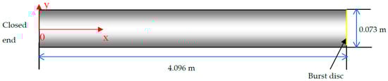
Figure 1.
Edwards and O’Brien blowdown test.
The pipe was filled with sub-cooled water, whose initial conditions ranged from 3.55 MPa to 17.34 MPa and from 514.8 K to 616.5 K. At the burst of the glass disc, the depressurization wave propagates through the pipe, and water becomes superheated and vaporizes suddenly. Measurements were performed at several horizontal positions.
4.1.2. Simulation Results
The problem investigated in the present work has initial conditions of 7.00 MPa and 513.7 K. A pressure boundary was assumed for the outlet, and the background pressure was 1 atm. The simulation is done on a 3D cylinder grid, and furthermore, the five-equation model mentioned above with the prescribed bubble diameter (dg = 1 mm) as in [3] is applied. The results of absolute pressure and void fraction at the position x = 1.469 m are presented in Figure 2a,b and compared with the experimental data.
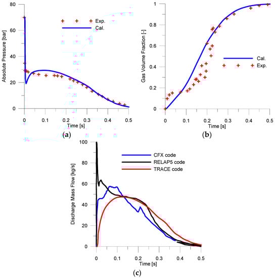
Figure 2.
Evolution of flow parameters at x = 1.469 m after the disc burst: (a) absolute pressure; (b) void fraction; (c) discharged mass flow rate change with the time.
One can see that the water inside the pipe vaporizes completely within a half second after the burst of the glass disc. The agreement between simulation and measurement is acceptable, especially at the later stage. In contrast, considerable deviations are present at the early stage of depressurization. The lowest pressure in the simulation, which corresponds to the maximum superheat degree and is required to trigger the onset of flashing, is obviously lower than that in the measurement. Furthermore, the rate of vapor production is under-predicted at the beginning, while in the period from 0.1 s to 0.2 s, it is over-predicted. It is acknowledged that the simplifying assumption of a constant mean bubble size is responsible for the deviations. It is inconsistent with the physical picture of the process, although it is widely used. The size of pre-existing nuclei in the sub-cooled liquid is substantially smaller than the prescribed value of 1 mm. This indicates a significant under-prediction of interfacial area density available for the initiation of flashing. On the other hand, steam bubbles grow rapidly during the flashing process, leading to a mean size much larger than 1 mm in a short time. Nevertheless, the effect of this uncertainty is weakened with the increase of the void fraction. The effect of prescribed bubble size was investigated in [27].
The discharged mass flow from the blowdown pipe is shown in Figure 2c below. Due to lack of experimental information, the results are compared with those obtained by two classical system codes, i.e., RELAP5 and TRACE, from the recent work [28]. One can see that the maximum value is reached shortly after the burst, where the difference between the codes is largest. According to RELAP5, the mass flow increases rapidly from 0 to 100 kg/s at the moment of the burst, while TRACE and CFX give a significantly lower maximum value with a delay around 0.1 s. In addition, the change of mass the flow rate with time delivered by CFX is much more gentle and smooth in comparison to that by RELAP5 and CFX.
4.2. Flashing-Induced Instability Problem in Natural Circulation
4.2.1. Description of the Problem
Since the middle of the 1980s, it has been recognized that the application of passive safety systems can contribute to improving the economics and reliability of nuclear power plants. In some advanced designs, natural circulation is used as a means for residual heat removal. For example, in a German BWR (boiling water reactor) concept, namely, the KERENA™ reactor [29], the containment cooling condenser (CCC) is the key component of a natural cooling circuit; see the red shaded region in Figure 3. In the case of overpressure, surplus steam in the containment condenses on the outside wall of CCC. Heat released by condensation is transferred to the cooling water inside the CCC tubes and finally to the shielding/storage pool vessel (SSPV) through natural circulation.
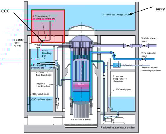
Figure 3.
Section picture of KERENA™ containment [30]. CCC: containment cooling condenser; SSPV: shielding/storage pool vessel.
In the experimental investigation performed by AREVA [30], a severe water hammer was experienced. The flow instability is believed to come from the rapid formation and subsequent destruction of steam bubbles inside the circuit. Natural circulation systems are characterized by a downcomer and a riser, which connect to a heated and a cooled section at the ends, respectively. Nearly saturated warm circulating water can flash to vapor inside the riser if no boiling occurs in the heated section. Liquid temperature remains constant till flashing begins if the heat loss through the riser is negligible (adiabatic), while saturation temperature decreases with increased altitude.
The production of vapor in a flashing process taking place in natural circulation has a periodic oscillation character [31]. The circulation flow rate increases as a result of vapor production, which further leads to a low liquid temperature entering the riser. It can be lower than the saturation temperature at the exit of the riser. As a consequence, the flashing is suppressed, which leads to a decrease in flow rate and subsequently an increase in liquid temperature. Therefore, flashing can take place again in the adiabatic riser and generates a self-sustained oscillating flow. The feature of high frequency oscillation and rapid phase change requires high resolution and can cause numerical instability and convergence problems in high-resolved CFD simulations.
4.2.2. Simulation Results
For the simulation, a 3D pipe section is constructed on the basis of the riser in the AREVA test facility; see Figure 4. Two inlets are connected to two CCC condensers. For details on the experiments please, refer to [27,29]. Boundary conditions, such as inlet temperature, mass flow rate and outlet pressure level are provided by the experimental data. Furthermore, the single-phase condition at the inlet is assured by choosing a proper time segment according to the measurement. The start time for simulation is chosen as 4600 s. Furthermore, a mono-disperse approach is utilized, which distinguishes itself from the last case by the prescription of bubble number density instead of bubble size. A constant value of 5 × 10⁴ m−3 is assumed in the following simulation. The settings are believed to be closer to the physical process of flashing since the bubbles are allowed to grow [4].
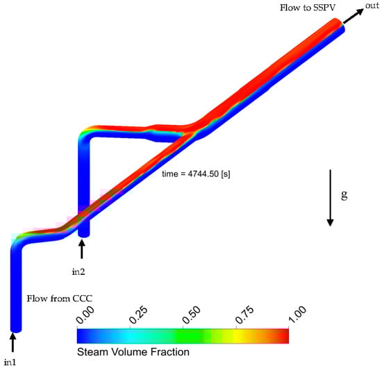
Figure 4.
Segment of the riser pipe applied in the simulation colored by steam volume fraction at t = 4744.50 s.
Figure 4 shows the distribution of steam inside the domain at the moment of 4744.50 s. The red color symbolizes steam, while the blue is water. As discussed above, the liquid at the exit becomes first superheated and initiates the flashing process. This gives rise to a high steam volume fraction at the upper part, while single phase flow exists still in the two straight legs near the inlets. Since the gravitational force is considered, steam is accumulated at the top side of the inclined pipe leading to a stratified flow pattern. A broad range of flow patterns and regime transition represents challenges for current two-phase CFD technology.
The temporal course of the inlet pressure and liquid temperature (the measured pressure at the outlet and temperature at the inlet are given as boundary conditions) is depicted in Figure 5. During the time segment from 4600 s to 5200 s, the production of vapor goes periodically through onset, intensification and ceasing, and thermo-hydraulic parameters oscillate correspondingly. The maximum amplitude of pressure and temperature oscillation can reach 0.8 bar and 50 K, respectively. The predicted period agrees well with the measured one, and the amplitude of temperature profile is also satisfying. Nevertheless, clear deviation is observed at pressure valleys, where the onset of flashing occurs. Similar to the limitation of the last method with constant bubble size, the disagreement results from the prescription of a constant bubble number density and neglecting bubble dynamics, such as coalescence and break-up. The sensitivity study on the prescribed values for bubble number density was performed in the previous work of [32].
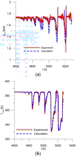
Figure 5.
Comparison between calculation and experiment: (a) inlet pressure; (b) outlet temperature.
4.3. Abuaf [33] Nozzle Flashing Flow Test
4.3.1. Description of the Test
In nuclear safety analysis, the flashing of initially sub-cooled liquid through nozzles, orifices or other restrictions has been studied intensively for several decades due to the design basic accident of LOCA (loss-of-coolant accident). Much attention was paid to the critical flow problem, while a deep insight into the transient development of two-phase flow structure is still missing. In comparison with the single phase, the complexity of two-phase critical flow arises from both thermal and mechanical non-equilibrium effects at the interface, which prevent reliable prediction of the critical flow rate from using empirical relations.
The experimental investigation of water flashing through a converging-diverging nozzle presented in [33] has been widely used as a reference for numerical study or model development, e.g., [7,34]. In the frame of this work, several tests with different boundary conditions, such as inlet pressure, temperature and outlet pressure, are reproduced by means of CFD technology. The geometrical sketch of the circular nozzle is shown in Figure 6. Dynamic pressure decreases with the reduction of channel area in the converging part leading to a decrease in the saturation temperature. If it falls below the liquid temperature before reaching the neck position, the onset of flashing will occur near the neck and vaporization continues in the diverging part.
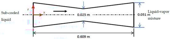
Figure 6.
Circular converging-diverging nozzle used in the tests of [33].
4.3.2. Simulation Results
For this case, the generation and transportation of bubbles is traced by solving an additional transport equation for bubble number density. Similar setups were adopted in [6,7]; see Table 1. The formation of bubbles in superheated liquid is called “nucleation”, which is deemed to take place under two different mechanisms, namely homogeneous and heterogeneous nucleation. Homogeneous nucleation occurs uniformly in the bulk caused by the thermodynamic state fluctuation of liquid molecules. In contrast, heterogeneous nucleation takes place at foreign “nuclei”, which can be microscopic cavities on solid walls or dissolved gasses and impurities pre-existing in the sub-cooled liquid. The latter mechanism has been recognized to be dominant in the real processes, which is therefore taken into account in the current work. Since it allows both bubble size and number to vary, this method is obviously stepwise superior to the previous ones with prescribed bubble size or number density. However, it requires one more closure model, namely the nucleation model, which is still one weak spot in the numerical study of the boiling process. For investigations on the effect of nucleation models, please refer to [9].
From the spatial distribution of steam shown in Figure 7, one can see that the onset of vaporization occurs near the nozzle neck, and bubbles are formed overwhelmingly at the walls and then migrate to the center region. In other words, the mechanism of wall nucleation is dominant in comparison to bulk heterogeneous nucleation. As a result, the radial profile with a clear wall peak is built. The example presented below Figure 8, Figure 9 and Figure 10 has the boundary conditions of inlet pressure 555.9 kPa, outlet pressure 402.5 kPa and inlet temperature 422.25 K.
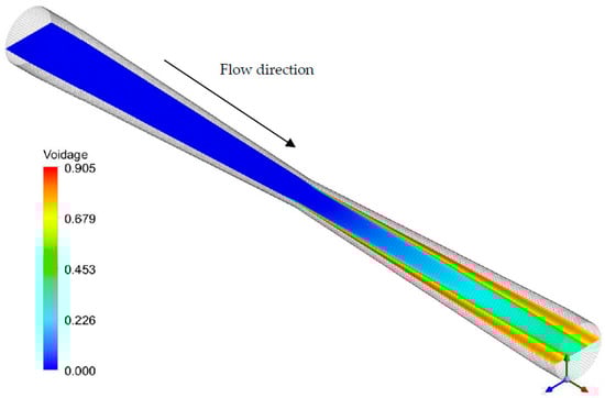
Figure 7.
Distribution of the steam volume fraction inside the nozzle.
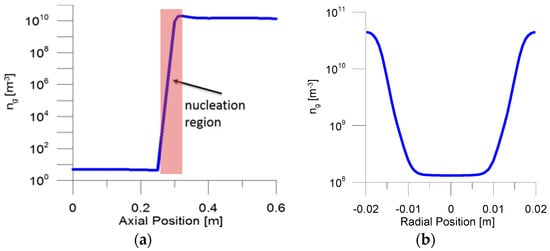
Figure 8.
Distribution of bubble number density in (a) the axial direction and (b) the radial direction at x = 0.458 m.
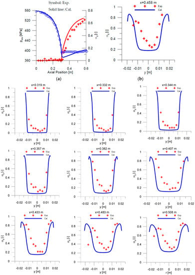
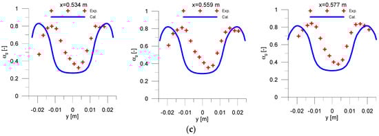
Figure 9.
Comparison between calculation and experiment: (a) axial profile of the pressure and void fraction; (b) radial profile of the void fraction; (c) radial profile of the void fraction at different axial positions.
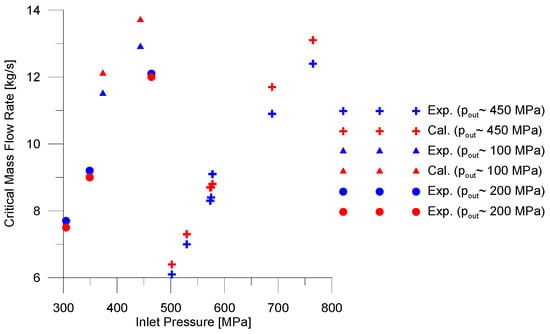
Figure 10.
Dependence of the critical mass flow rate on inlet and outlet pressure in the nozzle.
Furthermore, the nucleation process is found to take place in a narrow region (a few centimeters); see the red shaded region in Figure 8a. The cross-section averaged bubble number density increases steeply in the nucleation region and then remains almost constant in the stable two-phase region. The models described in [16,21] are chosen for the computation of the heterogeneous nucleation rate at the walls and in the bulk. The contribution of bulk nucleation is found to be trivial. In addition, the assumed small initial value is proven to have no influence on the final results [9].
The radial profile of bubble distribution in Figure 8b shows that the majority of steam bubbles remain in the neighborhood of nucleation spots (here, wall cavities), and the concentration in the center region is low and flat. The rate of bubbles migrating from the near-wall region to the nozzle center increases with the bubble size.
In Figure 9, the simulation results are compared with the data. On the left side is the axial profile of absolute pressure (left y-axis) and steam volume fraction (right y-axis), and on the right side is the radial profile of the steam volume fraction at the position x = 0.458 m. Symbols and lines represent measurement and calculation, respectively.
The cross-section averaged steam volume fraction increases in the latter part of flow path, which is in an acceptable agreement with the data. On the other hand, the pressure profile exhibits obvious deviations in the diverging part of the nozzle. The predicted value is lower than the measured one. It suggests that too high a superheat (or pressure undershoot) is required for triggering the onset of flashing in comparison to the experiment. In other words, with the same superheat degree as observed in the experiment, the predicted inter-phase heat transfer rate is insufficient to overcome the latent heat and keep bubbles stable. The interfacial area density or inter-phase heat transfer coefficient is under-predicted at the moment of flashing onset. After triggering the flashing process, the pressure increases under the constraint of the outlet pressure, which is given as the boundary condition. Furthermore, the assumption of pressure equilibrium across the interface might introduce large errors in high pressure undershoot cases.
The transverse distribution of bubbles in the continuous medium is determined by non-drag forces, which depend sensitively on the mean bubble size. It is determined by the bubble number density and nucleation rate, since bubble coalescence and break-up are not considered. As shown in Figure 8b and Figure 9b, bubbles are formed and accumulated in the near wall region and create a void fraction profile with a high wall-peak while a low value in the center region. A similar profile is obtained in the measurement. However, it displays a more gradual transition from the wall peak to the center valley. That means that more bubbles have migrated to the center due to the effect of non-drag forces, i.e., lift and turbulence dispersion. This may imply that bubble growth is under-estimated, and coalescence effects should be taken into account, since lift force pushes large bubbles to the center, while small bubbles to the wall. However, to refine the results, reliable data of local bubble size distributions are indispensable, which are unfortunately missing in most experimental investigations. Furthermore, sufficient turbulent dispersion would also help to improve the agreement. According to the FAD (Favre averaged drag) model, the dispersion force is proportional to eddy viscosity, which is probably under-predicted by the SST model with BIT source terms.
To give more details about the flow structure, the radial profile of the void fraction is depicted in Figure 9c for several axial positions other than x = 0.458 m shown above. The formation of bubbles starts around the throat position (x = 0.305 m; see Figure 6) and first leads to a monotonous peak near the wall. It shifts slowly to the nozzle center due to the effect of non-drag forces along the axis, and an “M-shape” profile is developed over the cross-section. The simulated results agree well with the measured ones except for an over-prediction of the wall-peak at the beginning. Another important observation is that in the experiment, the profile is not symmetrical with respect to the axis. According to the experimenter, the asymmetry might be due to the presence of pressure taps on one side of the nozzle [33], which act as nucleation centers.
Several other tests with different inlet and outlet pressures, as well as inlet temperatures are simulated. The critical mass flow rates are summarized in Figure 10 below. The critical rate of flow through the nozzle depends on a variety of parameters, inlet pressure, quality, pressure-undershoot, and so on. In general, increasing the inlet stagnation pressure or decreasing outlet pressure leads to an increase in the critical mass flow rate. Furthermore, the presence of vapor reduces the average density of the two-phase mixture and, thus, favors the deceleration process in the diverging part of the nozzle.
It is shown that the simulated results are in an overall good agreement with the measured ones. The maximum deviation is within 7%. Nevertheless, the simulation tends to under-predict the critical mass flow rate with the increasing of the inlet pressure and decreasing of the outlet pressure.
5. Poly-Disperse Simulations
Although it is commonly used, the mono-disperse approach presented above is self-evident limited to situations with a constant bubble size or a narrow distribution. On the other hand, flashing processes are always accompanied with rapid vaporization and a high void fraction. This suggests that a broad spectrum of bubble sizes can be present, which asks for a poly-disperse simulation method. However, to the author’s knowledge, no publications in this aspect are so far available for flashing situations, although there is a wide range of poly-disperse simulations for isothermal flows and a few for sub-cooled boiling.
In this work, the first attempts are made to apply the inhomogeneous MUSIG (multiple size group) model [35,36] to controlled pressure release transients, which were carried out on the TOPFLOW facility (see below). MUSIG is a poly-disperse method available in CFX for computing the mean bubble size of a spectrum. It is one kind of class method approximating the size spectrum with several discrete classes; see Figure 11.
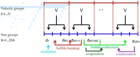
Figure 11.
Schema of the inhomogeneous multiple size group (MUSIG) model.
The division of size groups is finer than that of velocity groups due to the limitation of computational speed. Separate momentum equations are solved for each velocity group while all phenomena that change the size distribution, such as nucleation, coalescence and breakup, are considered within the sub-size groups. The exchange between these size groups due to the above-mentioned phenomena is reproduced by solving additional transport equations with corresponding source/sink terms for the fraction of each group fi. As a result, the mean Sauter diameter of bubbles belonging to a velocity group can be obtained from these size fractions. The MUSIG approach has been expounded in detail elsewhere [24,36].
5.1. TOPFLOW Pressure Release Experiment
One major test section equipped in the TOPFLOW facility is a vertical pipe with a nominal diameter of 200 mm; see Figure 12. The pressure release experiment was carried out at this section. For details about the multipurpose thermal-hydraulic test facility TOPFLOW at Helmholtz-Zentrum Dresden-Rossendorf, please refer to the work of [37].
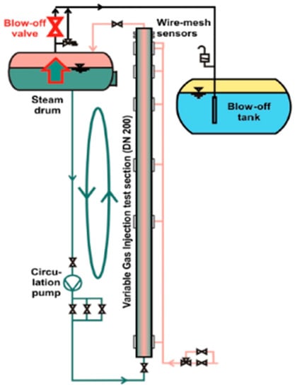
Figure 12.
Schema of the experimental procedure.
During the pressure release experiment, water was circulated with a velocity of about 1 m/s and flows upwards through the test section; see Figure 12. The transient pressure course is controlled by the blow-off valve located above the steam drum, where saturation conditions are always guaranteed. As a result, cavitation in the circulation pump below is avoided. At the same time, the maximum evaporation rate in the test section is limited [27].
The blow-off valve was opened to a maximum level and closed again according to the ramp shape as shown in Figure 13.
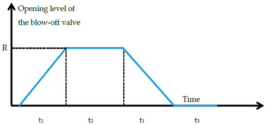
Figure 13.
Operation of the blow-off valve.
The operation speed of the valve is controlled by time t1, while the maximum opening degree and its duration are represented by R and t2. Correspondingly, the generation and disappearance of steam inside the pipe are determined by the pressure release rate and the operation of the valve. Measurements of the volume fraction, gas velocity and bubble size distribution were realized with the aid of wire-mesh sensors (WMS) at the top; see Figure 12. The highly-resolved data of bubble size distributions and radial void fractions are optimal for the validation of simulation results obtained by the poly-disperse method. Rapid expansion of bubbles and a broad size spectrum were observed in the experiment, and for reliable simulation results, it is necessary to use a poly-disperse method. A detailed introduction to the experimental procedure and discussion on the influence of pressure level on the data were given by Lucas [38].
Two test cases under different pressure levels are investigated in the current work, whose experimental conditions are summarized in Table 2 below.
Table 2.
Experimental conditions of the investigated test cases.
Measured inlet temperature, mass flow rate and outlet pressure are used as boundary conditions in the simulation.
5.2. Simulation Results
The aim of poly-disperse simulations is to obtain a realistic mean bubble size by tracing the dynamic change of bubble size distributions, which is important in the case of a broad bubble size spectrum. For this purpose, besides highly-resolved data, reliable closure models for all physical processes that affect the bubble size are indispensable. In this work not only nucleation and phase change, but also bubble coalescence and break-up have been taken into account (see Figure 11). For heterogeneous nucleation, the same models as for the nozzle flow discussed above in Section 4.3.2 were employed, while the models presented in [24] were used for bubble coalescence and break-up. The change resulting from these phenomena is implemented as source or sink in the MUSIG size fraction transport equations mentioned above.
The evolution of the normalized bubble size distribution is displayed in Figure 14 and Figure 15 for the two cases listed in Table 2, respectively. In the vertical axis label, ∆αi represents the void fraction portion belonging to the size group i, while ∑∆αi is the total void fraction. The red line represents experimental data, while the blue one simulation results.
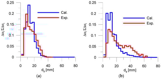
Figure 14.
Evolution of normalized bubble size distribution at the wire-mesh sensor (WMS) plane (Case 1): (a) t = 39 s; (b) t = 45 s.
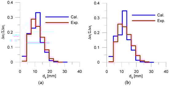
Figure 15.
Evolution of normalized bubble size distribution at the WMS plane (Case 2): (a) t = 29 s; (b) t = 49 s.
In Case 1, whose pressure level is 10 bar, bubble growth within the period from t = 39 s to 45 s is significant. The agreement between calculation and experiment at t = 39 s is satisfying, whereas six seconds later, the fraction of large bubbles is obviously under-predicted. As a result, the mean bubble size is smaller than the measured one, although both of them increase. One possible reason for this discrepancy is that the mechanism for inter-phase mass transfer is not completely reproduced by the “thermal phase change model”. Furthermore, the break-up rate of large bubbles may be overestimated corresponding to the coalescence rate of small bubbles. The predictability of coalescence and break-up models depends on a number of input parameters, such as turbulence intensity and interfacial shear stress. The evaluation of these parameters in such complex two-phase flows is often difficult. In addition, the superposition of various mechanisms, as well as of coalescence and break-up effects increases the difficulty in further development and improvement of these closures.
The growth of bubbles is substantially slowed down with the increase of pressure level. As shown in Figure 15, in Case 2, the change of bubble size distribution within 20 s is trivial. Consequently, the agreement at both time points is acceptable.
The different performance of the applied model setup at two pressure levels suggests that the contribution of pressure non-equilibrium at the interface to inter-phase mass transfer can be significant in Case 1. An approach that takes both thermal and mechanical non-equilibrium into account is necessary to ensure the reliability of predictions in both low and high pressures.
The pressure and velocity field shown in Figure 16 and Figure 17 below is intended to provide further insight into the flashing flow. In the simulation, the pressure boundary condition was specified for the outlet (top), and the measured pressure was imposed on the boundary. The calculated pressure at the inlet (bottom) was found in good agreement with the data, as shown in Figure 16. This implies that the pressure field in the whole domain is well reproduced. Water flashes into steam during the depressurization, whose rate is controlled by the opening of the blow-off valve (see Figure 13).
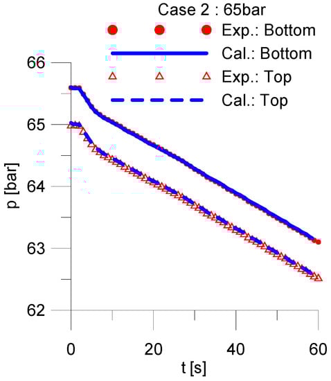
Figure 16.
Evolution of the cross-section averaged absolute pressure at the top and bottom of the test section (Case 2).
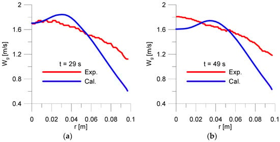
Figure 17.
Evolution of radial gas velocity profiles at the WMS plane (Case 2): (a) t = 29 s; (b) t = 49 s.
The comparison of the gas vertical velocity component at the WMS plane, where data are available, is shown in Figure 17. Instead of a core peak as observed in the measurement, the calculated radial profiles show a transit peak. The velocity profile is similar to the void fraction ones, which depends on the magnitude of non-drag forces. Since the bubble size is well captured (see Figure 15), the discrepancy is caused either by an under-prediction of turbulence dispersion force or an over-prediction of lift force. Under the role of lift force, large bubbles move away from the wall and accumulate in the center, while turbulence dispersion tends to counteract this effect. However, for further evaluation of these models, reliable reference information, e.g., turbulence, is still missing.
Improving the two-phase turbulence, as well as dispersion and lift force modelling will be one of the emphases of future work. Related theoretical and experimental work has been planned and begun.
6. Conclusions
Flashing of liquid to vapor due to pressure drop represents highly complex two-phase situations. Due to its relevance to nuclear safety analysis, the flashing phenomenon has been extensively studied for several decades. Nevertheless, there exists a need to update the analytical approach to a sophistication level that matches available computational technologies, e.g., from system codes to CFD codes. CFD simulations with the simplified mono-disperse approaches, which are commonly used and often deliver satisfying results, are however limited for cases with nearly constant bubble size or number density. Since these conditions are normally not fulfilled, they are shown to have difficulty in capturing the onset of flashing, which consequently affects the agreement in the subsequent phase change stage. In addition, the results are sensitively dependent on the prescribed values and the spatial distribution of phases on the mean bubble size. The poly-disperse approach is promising for removing these restrictions, since it is free of any open parameters and reproduces the realistic change of bubble size distributions. However, as suggested in [12], more elaborate models require more empirical correlations or assumptions for phase interactions which are so far insufficiently tested. As a result, the prediction accuracy of the sophisticated method is greatly affected.
Therefore, before we can exploit the benefits of CFD simulations for flashing flows, we have to understand the physical sub-phenomena, such as nucleation characteristics and inter-phase transfer laws sufficiently, and be able to specify them precisely with closure models. For this purpose, highly-resolved and comprehensive data achieved by experiments or direct numerical simulations are indispensable, especially local bubble size, phase distribution, turbulence, velocity and pressure fields, which are often unavailable, e.g., in Tests 4.1, 4.2 and 4.3. The wire-mesh senor technique applied in the TOPFLOW pressure release experiment can provide the above measurements. Nevertheless, the necessary information on liquid velocity and turbulence parameters is still missing. The development of new measurement techniques is undergoing [39].
The presented results show that the Eulerian CFD technology reproduces global parameters, such as pressure and flow rates, reliably, even in complex practical situations. Nevertheless, the prediction of local phenomena, e.g., phase distribution and velocity fields, is still insufficient. More efforts are required in the assessment and improvement of closures.
Acknowledgments
This work was carried out at Helmholtz-Zentrum Dresden-Rossendorf in the frame of a research project funded by EON Kernkraft GmbH.
Author Contributions
Dirk Lucas and Yixiang Liao conceived of the simulations and evaluated the results. Yixiang Liao performed the simulations and wrote the paper.
Conflicts of Interest
The authors declare that there is no conflict of interest regarding the publication of this paper. The founding sponsors had no role in the design of the study; in the collection, analyses, or interpretation of data; in the writing of the manuscript, and in the decision to publish the results.
Abbreviations
| ANSYS | an American computer-aided engineering software developer headquartered south of Pittsburgh in Cecil Township, Pennsylvania, United States |
| AREVA | a French multinational group specializing in nuclear power and renewable energy headquartered in Paris La Défense |
| CCC | containment cooling condenser, a passive nuclear safety system |
| CFD | computational fluid dynamics |
| CFX | a commercial CFD code developed by ANSYS company |
| CSNI | committee on the Safety of Nuclear Installations, a committee of the OECD/NEA |
| FLUENT | a commercial CFD code developed by ANSYS company |
| IAPWS-IF97 | International Association for the Properties of Water and Steam – Industrial Formulation 1997 |
| KERENATM | a mid-power boiling water reactor developed jointly by the AREVA company and the German energy supply company E.ON |
| NEA | Nuclear Energy Agency, an intergovernmental agency organized under OECD |
| NEPTUNE-CFD | a French code created by EDF (Électricité de France) and CEA (Commissariat à I’Energie Atomique) for nuclear reactor thermal-hydraulics simulation and analyses |
| OECD | Organization for Economic Co-operation and Development |
| RELAP5 | abbreviation of “Reactor Excursion and Leak Analysis Program”, A component-oriented reactor systems thermal-hydraulics analysis code developed at Idaho National Laboratory |
| RPI | Rensselaer Polytechnic Institute |
| SSPV | Shielding/Storage Pool Vessel in KENERA reactor |
| TRACE | TRAC/RELAP Advanced Computational Engine, a component-oriented reactor systems thermal-hydraulics analysis code |
| TRAC | transient reactor analysis code, another reactor system code |
| WMS | wire mesh sensor, a measurement technique |
References
- Giese, T.; Laurien, E. A thermal based model for cavitation in saturated liquids. Z. Angew. Math. Mech. 2001, 81, 957–958. [Google Scholar]
- Giese, T.; Laurien, E. Experimental and numerical investigation of gravity-driven pipe flow with cavitation. In Proceedings of the 10th International Conference on Nuclear Engineering (ICONE10), Arlington, VA, USA, 14–18 April 2002.
- Laurien, E.; Giese, T. Exploration of the two fluid model of two-phase flow towards boiling, cavitation and stratification. In Proceedings of the 3rd International Conference on Computational Heat and Mass Transfer, Banff, AB, Canada, 26–30 May 2003.
- Laurien, E. Influence of the model bubble diameter on three-dimensional numerical simulations of thermal cavitation in pipe elbows. In Proceedings of the 3rd International Symposium on Two-Phase Flow Modelling and Experimentation, Pisa, Italy, 22–24 September 2004.
- Frank, T. Simulation of flashing and steam condensation in subcooled liquid using ANSYS CFX. In Proceedings of the 5th Joint FZR & ANSYS Workshop “Multiphase Flows: Simulation, Experiment and Application”, Dresden, Germany, 26–27 April 2007.
- Maksic, S.; Mewes, D. CFD-Calculation of the flashing flow in pipes and nozzles. In Proceedings of the Joint U.S.—European Fluids Engineering Division Conference (ASME FEDSM’02), Montreal, QC, Canada, 14–18 July 2002.
- Marsh, C.A.; O’Mahony, A.P. Three-dimensional modelling of industrial flashing flows. In Proceedings of the Computational Fluid Dynamics (CFD 2008), Trondheim, Norway, 10–12 June 2008.
- Mimouni, S.; Boucker, M.; Laviéville, J.; Guelfi, A.; Bestion, D. Modelling and computation of cavitation and boiling bubbly flows with the NEPTUNE_CFD code. Nucl. Eng. Des. 2008, 238, 680–692. [Google Scholar] [CrossRef]
- Janet, J.P.; Liao, Y.; Lucas, D. Heterogeneous nucleation in CFD simulation of flashing flows in converging-diverging nozzles. Int. J. Multiph. Flow 2015, 74, 106–117. [Google Scholar] [CrossRef]
- Edwards, A.R.; O’Brien, T.P. Studies of phenomena connected with the depressurization of water reactors. J. Br. Nucl. Enery Soc. 1970, 9, 125–135. [Google Scholar]
- Liao, Y.; Lucas, D.; Krepper, E.; Rzehak, R. Assessment of CFD predictive capacity for flash boiling. In Proceedings of the Computational Fluid Dynamics for Nuclear Reactor Safety-5 (CFD4NRS-5), Zurich, Switzerland, 9–11 September 2014.
- Wallis, G.B. Critical two-phase flow. Int. J. Multiph. Flow 1980, 6, 97–112. [Google Scholar] [CrossRef]
- Jones, O.C., Jr.; Zuber, N. Bubble growth in variable pressure fields. J. Heat Transf. 1978, 100, 453–459. [Google Scholar] [CrossRef]
- Shin, T.S.; Jones, O.C., Jr. An active cavity model for flashing. Nucl. Eng. Des. 1986, 95, 185–196. [Google Scholar] [CrossRef]
- Shin, T.S.; Jones, O.C. Nucleation and flashing in nozzles—1. Int. J. Multiph. Flow 1993, 19, 943–964. [Google Scholar] [CrossRef]
- Blinkov, V.N.; Jones, O.C.; Nigmatulin, B.I. Nucleation and flashing in nozzles—2. Int. J. Multiph. Flow 1993, 19, 965–986. [Google Scholar] [CrossRef]
- Blander, M.; Katz, J.L. Bubble nucleation in liquids. AIChE J. 1975, 21, 833–848. [Google Scholar] [CrossRef]
- Release 14.5. ANSYS CFX-Solver Theory Guide; ANSYS: Canonsburg, PA, USA, 2012.
- Riznic, J.; Ishii, M. Bubble number density in vapor generation and flashing flow. Int. J. Heat Mass Transf. 1989, 32, 1821–1833. [Google Scholar] [CrossRef]
- Ranz, W.E.; Marshall, W.R. Evaporation from drops—Part I. Chem. Eng. Prog. 1952, 48, 141–146. [Google Scholar]
- Ranz, W.E.; Marshall, W.R. Evaporation from drops—Part II. Chem. Eng. Prog. 1952, 48, 173–180. [Google Scholar]
- Rohatgi, U.; Reshotko, E. Non-equilibrium one-dimensional two-phase flow in variable area channels. In Non-Equilibrium Two-Phase Flows, Proceedings of the Winter Annual Meeting, Houston, TX, USA, 30 November–5 December 1975; Meeting Sponsored by the American Society of Mechanical Engineers; American Society of Mechanical Engineers: New York, NY, USA, 1975; Volume 1, pp. 47–54. [Google Scholar]
- Rzehak, R.; Krepper, E. CFD modeling of bubble-induced turbulence. Int. J. Multiph. Flow 2013, 55, 138–155. [Google Scholar] [CrossRef]
- Liao, Y.; Rzehak, R.; Lucas, D.; Krepper, E. Baseline closure model for dispersed bubbly flow: Bubble coalescence and breakup. Chem. Eng. Sci. 2015, 122, 336–349. [Google Scholar] [CrossRef]
- Garner, R.W. Comparative Analyses of Standard Problems, Standard Problem 1 (Straight Pipe Depressurization Experiments); Interim Report I-212-74-5.1; Aerojet Nuclear Company: Rancho Cordova, CA, USA, 1973. [Google Scholar]
- Stello, V. Summary of All Participants Results in Comparison to the Experimental Data for the CSNI Standard Problem 1; For the CSNI-Ad Hoc Working Group on Emergency Core Cooling; OECD/NEA: Paris, Franch, 1975. [Google Scholar]
- Liao, Y.; Lucas, D.; Krepper, E.; Rzehak, R. Flashing evaporation under different pressure levels. Nucl. Eng. Des. 2013, 265, 801–813. [Google Scholar] [CrossRef]
- Gurgacz, S.; Pawluczyk, M.; Niewiński, G.; Mazgaj, P. Simulation and analysis of pipe and vessel blowdown phenomena using RELAP5 and TRACE. J. Power Technol. 2014, 94, 61–68. [Google Scholar]
- Dardy, A. The AREVA Reactor Range—The Nuclear Safety Reference for Europe; AREVA Day: Warsaw, Poland, 2010. [Google Scholar]
- Leyer, S.; Wich, M. The Integral test facility Karlstein. Sci. Technol. Nucl. Install. 2012, 2012, 439374. [Google Scholar] [CrossRef]
- Manera, A. Experimental and Analytical Investigations on Flashing-Induced Instabilities in Natural Circulation Two-Phase Systems. Ph.D. Thesis, Delft University of Technology, Delft, The Netherlands, 2003. [Google Scholar]
- Liao, Y.; Lucas, D. 3D CFD simulation of flashing flows in a converging-diverging nozzle. Nucl. Eng. Des. 2015, 292, 149–163. [Google Scholar] [CrossRef]
- Abuaf, N.; Wu, B.J.C.; Zimmer, G.A.; Saha, P. A Study of Nonequilibrium Flashing of Water in a Converging-Diverging Nozzle: Volume 1—Experimental; U.S. Nuclear Regulatory Commission: Washington, DC, USA, 1981.
- Riznic, J.; Ishii, M.; Afgan, N. Mechanistic model for void distribution in flashing flow. In Proceedings of the Transient Phenomena in Multiphase Flow (ICHMT Seminar), Dubrovnik, Yugoslavia, 24–30 May 1987.
- Krepper, E.; Lucas, D.; Frank, T.; Prasser, H.-M.; Zwart, P.J. The inhomogeneous MUSIG model for the simulation of polydispersed flows. Nucl. Eng. Des. 2008, 238, 1690–1702. [Google Scholar] [CrossRef]
- Liao, Y.; Lucas, D. Poly-disperse simulation of condensing steam-water flow inside a large vertical pipe. Int. J. Therm. Sci. 2016, 104, 194–207. [Google Scholar] [CrossRef]
- Schaffrath, A.; Kruessenberg, A.K.; Weiss, F.P.; Beyer, M.; Carl, H.; Prasser, H.M.; Schuster, J.; Schuetz, P.; Tamme, M.; Zimmermann, W. TOPFLOW—A new multipurpose thermalhydraulic test facility for the investigation of steady state and transient two-phase flow phenomena. Kerntechnik 2001, 66, 209–212. [Google Scholar]
- Lucas, D.; Beyer, M.; Szalinski, L. Experiments on evaporating pipe flow. In Proceedings of the 14th International Topical Meeting on Nuclear Reactor Thermalhydraulics (NURETH-14), Toronto, ON, Canada, 25–30 September 2011.
- Ziegenhein, T.; Zalucky, J.; Rzehak, R.; Lucas, D. On the hydrodynamics of airlift reactors, Part I: Experiments. Chem. Eng. Sci. 2016, 150, 54–65. [Google Scholar] [CrossRef]
© 2017 by the authors; licensee MDPI, Basel, Switzerland. This article is an open access article distributed under the terms and conditions of the Creative Commons Attribution (CC BY) license (http://creativecommons.org/licenses/by/4.0/).