Joint Analysis of Static and Dynamic Importance in the Eye-Tracking Records of Web Page Readers

Abstract

Heat maps highlight cumulative, static importance in eye-tracking records, while network analysis helps elucidate dynamic importance from transitional relations. The present study was designed to perform both analyses in the same conceptual framework, i.e., network representation. For this purpose, heat maps comprising 5 × 5 segments were overlaid with networks, both of which were produced from the eye-tracking records of 20 subjects who read 10 top web pages that were classified into three layout types. The heat of the segments was graded on the basis of five percentile scores, whereas the core-peripheral nodes were identified by the agreement of centrality and ranking indices. The congruence between the two types of importance was generally good at the node level and the community levels. Additional findings included a) mixed patterns of the sustained fixations (i.e., loops) within the total fixations, and b) an increase in reciprocity as the network scope was narrowed to communities and then to the core neighborhoods.

Introduction

Eye-tracking records of web page readers help reveal how much the readers were attracted by different areas of a given page and how their attention shifted among areas through the examination of, for example, heat maps (cumulative-static) and scan paths (relational-dynamic), respectively (see Nielsen et al., 2010 for introductory information). For these purposes, researchers may set a grid or mesh on a screen and count the number of eye fixations in the segments (see Granka et al., 2006; Josephson, 2004; Pan et al., 2004). If the goal of the analysis is to focus on content rather than location, the screen should be segmented by content. Although we employ a uniform grid in the present study to compare different pages, our approach is applicable to content-based segmentation as well.

Figure 1 shows a schematic illustration of the three basic methods for analyzing eye fixations, with uniform segmentation for ease of comparison. In the heat map, segments are colored according to the frequency of fixations: the higher the fixation frequency, the hotter is the segment (see Cutrell et al, 2007). Because it is static in nature, the map does not provide means to trace shifts in attention. To study this dynamic aspect, the scan path is a suitable choice. Drawing paths is simple, but one soon faces difficulties in analyzing multiple paths (Goldberg et al, 1999) owing to the lack of good summary indices other than length.

Network analysis fills the gap between these approaches, since it enables us to capture important segments in the transitional relations, as demonstrated by Matsuda and Takeuchi (2009, 2011), who examined eye-tracking records obtained from viewers of top pages of commercial web sites. They identified both core and peripheral segments on the basis of the centrality and ranking indices. Besides, they extracted communities from the union (U) of the cliques, i.e., complete subgraphs in which all nodes are connected. The network shown in Figure 1 gives a rough idea of a community, i.e., a densely connected subgraph, formed by large and brightly colored nodes. Their approach will be briefly explained next before we provide justification for the present study.

Network Analysis of the Eye-Fixation Data

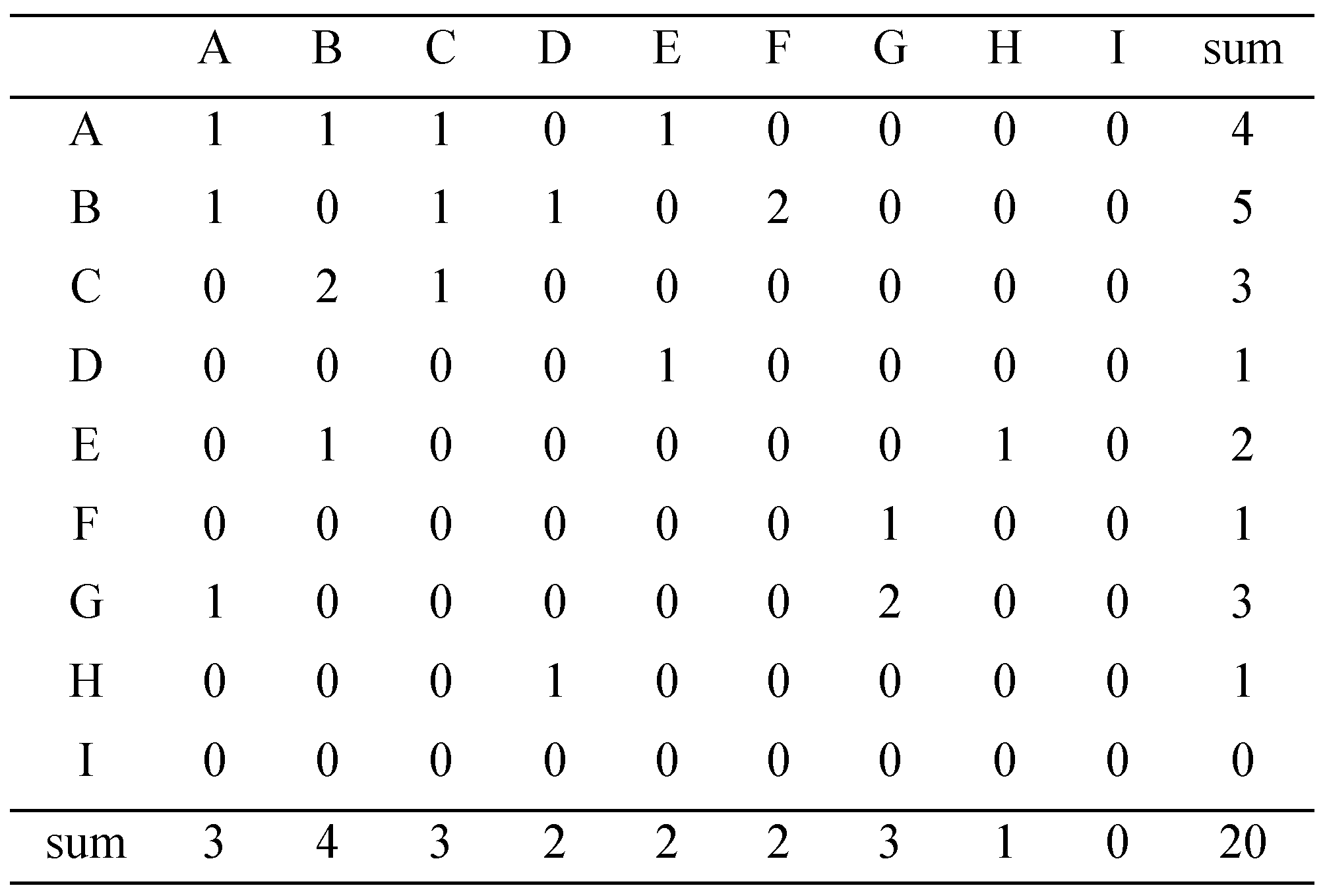
Matsuda et al. (2009, 2011) processed their analysis in four stages (see Appendix A of this paper for supplementary information): a) network construction, b) identification of core and peripheral nodes, c) identification of communities, and, d) visual presentation of the communities. First, the fixation sequences were transformed into adjacency matrices whose elements were the number of transitions between nodes. The diagonal elements corresponded to the self-loop transitions ("loops" for short). Networks of the nodes were constructed from each adjacency matrix.

Various network indices were computed in the second stage, including centralities and ranking scores. The most and least important nodes, referred to as core and peripheral nodes, respectively, were identified on the basis of the agreement of the ranks of these indices. In addition to selecting important individual nodes, Matsuda et al. attempted to extract communities defined as groups of nodes that were densely connected relative to those outside the group(s). In view of the small size of the networks (25 nodes), they formed a single community from the union (U) of the node sets that constituted the largest cliques in each network. Finally, they displayed the communities by the circular mode of Reingold and Tilford's (1981) tree layout algorithm, by placing the core nodes at the center.

Before introducing the motivation of the present study, more detailed explanation of the core (and peripheral) nodes would be necessary, in view of their special bearing on the dynamic importance.

Important Network Nodes

Few will disagree to attributing the importance of nodes to centrality: the greater the centrality of the node, the higher is its importance. However, the concept of centrality itself differs among three well-known centrality indices: degree, closeness, and betweenness (see Freeman, 1979, for the definitions). The two networks in Figure 2 are similar in that they both have three pivotal nodes {A, B, C} around which other nodes fan out.

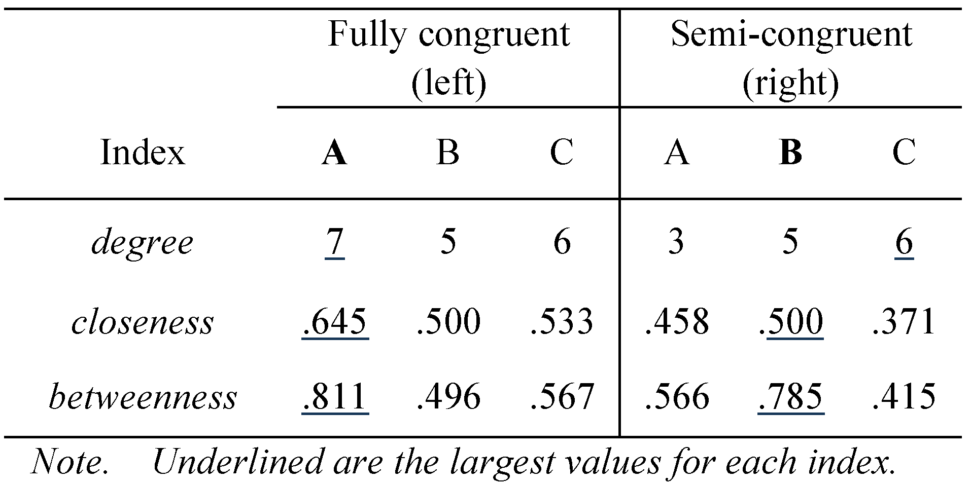
As listed in

Table 1. Centrality measures of the pivotal nodes. 

, node A in the left network is highly central, having the largest number of links connected to it (i.e., degree), being closest to the rest of the nodes in terms of geodesic distance (closeness), and having the largest proportion of short-cut paths running among all pairs of nodes (betweenness). In contrast, node A in the right network is not the most central, despite its middle position among the pivots. Here, C is highest in degree and B is highest in closeness and betweenness. If we were to determine the core status on the basis of congruence among these indices, A and B would be considered the core and semi-core in the left and right networks, respectively.

Besides the classical indices, the importance of nodes can be determined by the scores of PageRank (Brin et al, 1998) and the authority- and hub-scores (Kleinberg, 1999). They are essentially the values of the leading eigenvectors of the matrices differently derived from the adjacency matrix of a given network (see Appendix A, for additional note). Setting aside the mathematical details, what makes these ranking scores distinct from classical centrality measures is their recursive nature. That is, the importance of a node by PageRank depends on the importance of nodes connected to it, and the importance of these nodes further depends on nodes connected to them. The authority- and hub-scores bear mutually reinforcing relationships: The authoritativeness of a node is enhanced by the hubness of the nodes linking to it, while the hubness of a node increases as a function of the authoritativeness of the nodes they link to. We will select cores and peripherals on the basis of the agreement among the centrality indices and ranking scores, after Matsuda et al. (2009, 2011).

Motivations for the Joint Analysis

Although network analysis is useful, it is not sufficient by itself, owing to the difficulties in fully incorporating the static aspect, i.e., heat for two reasons. First, the fixation counts of the entry (or exit) segments are not retrievable from an adjacency matrix that records the number of shifts between the segments (see appendix A). Second, loops represented in the diagonal entries of the matrix cause complications in computing various indices and extracting communities. Hence, the removal of loops from network analysis is generally accepted as a means of avoiding substantial difficulties in interpreting the results. Moreover, loops are not distinguishable from recurrent fixations in heat maps unless specially separated. Therefore, their significance in terms of sustained interest deserves proper treatment to complement both the network approach and heat map analysis.

The purpose of the present analysis is to compare the two types of importance, one static and the other dynamic in nature, using the same records studied by Matsuda et al. (2009, 2011). Static importance, derived from the frequency of fixations, will be examined by heat maps and loops, while dynamic importance, derived from transitional relations, will be analyzed by the core and peripheral nodes. Our relational analysis will be extended to the clique-based communities (see Appendix A) containing the respective cores after the previous work. In addition, we will further narrow the scope of the networks to core neighborhoods comprising the nodes directly linked to and/or from the cores. The neighborhoods were displayed but not examined in the previous study.

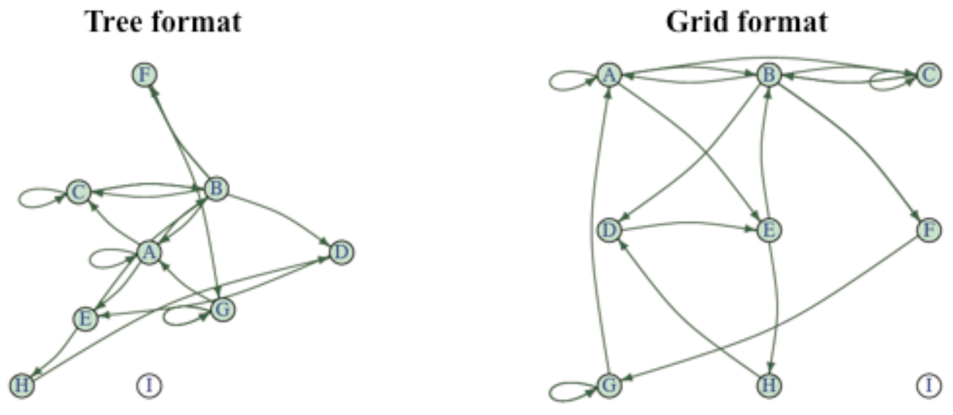
In order to facilitate the joint analysis, networks will be overlaid on the corresponding heat maps. To this end, we will depart in two ways from Matsuda et al. (2009, 2011) who displayed the communities alone, using the circular mode of Reingold and Tilford's (1981) tree layout algorithm. On the one hand, the entire network will be displayed with emphasis on the embedded communities and core-peripheral nodes. On the other, the networks will be displayed in grid form in correspondence to the segmentation of the screen (see Appendix A). The key to presenting the networks over the heat maps is our idea of also treating the latter as unconnected networks devoid of links.

Our study is expected to provide new analytical tools to both researchers and practitioners.

Method

Subjects (Ss). Twenty residents, (7 males and 13 females), living near a research institute called AIST, Japan, were recruited for the experiments. They had normal or corrected vision, and their ages ranged from 19 to 48 years (30 on the average). Ten of the Ss were university students, five were housewives, and the rest were parttime job holders. Eleven Ss were heavy Internet users, while the rest were light users, as judged from their reports about the number of hours they spent browsing in a week.

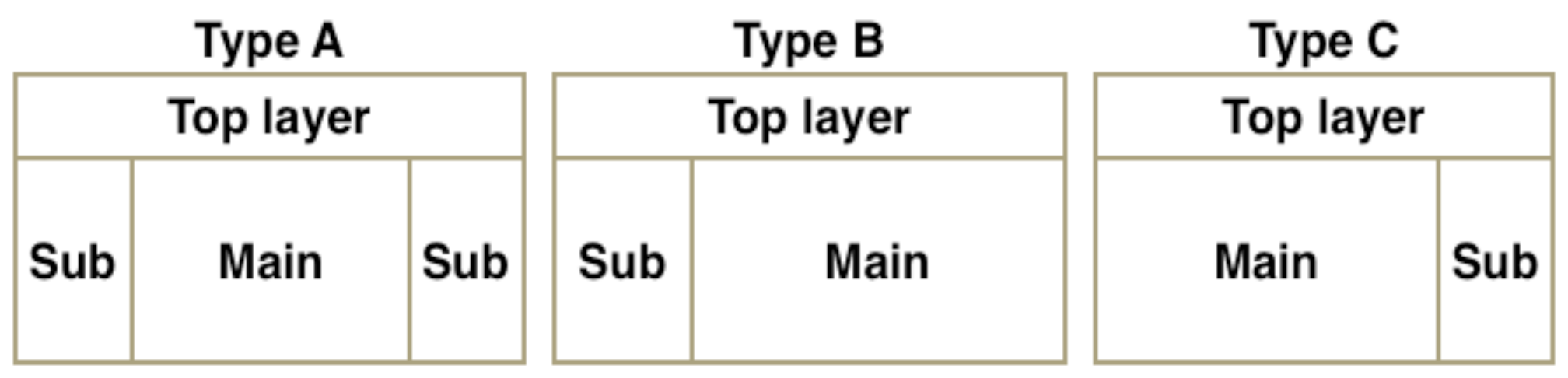
Stimuli. The top pages of ten commercial web sites were selected from various business areas: airline, ecommerce, finance, and banking. The pages were classified into Types A, B, and C, which differed in the layout of the principal part beneath the top layer (see Figure 3). The main area of Type A was sandwiched between sub-areas, while the main areas of Types B and C were accompanied by a single sub-area either on the left (B) or on the right (C).

Apparatus and procedure. The stimuli were presented with 1024 × 768 pixel resolution on a TFT 17” display of a Tobii 1750 eye-tracking system at the rate of 50 Hz. The web pages were randomly displayed to the Ss one at a time, each display lasting 20 sec. The Ss were asked to browse each page at their own pace. The English translation of the instructions is “Various Web pages will be shown on the computer display in turn. Please look at each page as you usually do until the screen darkens. Then, click the mouse button when you are ready to proceed.” The Ss were informed that the experiment would last approximately five minutes.

Segment coding and fixation sequences. A 5 × 5 mesh was imposed on the effective part of the screen stripped of white margins that had no text or graphics.

The segments were sequentially coded, as shown in Figure 4, by the combination of alphabetical and numerical labels for rows and columns, respectively: A1, A2, …, A5 for the first row; B1, …, B5 for the second; …; and E1, …, E5 for the fifth.

The raw tracking data for each subject comprised time-stamped xy-coordinates and were transformed to the fixation points under the condition that the subject’s eyes stayed within a radius of 30 pixels for a 100-msec period. Then, each fixation record was translated into code sequences according to the segments in which the fixation points fell.

Adjacency (Transition) matrix. An adjacency matrix (25 × 25) was constructed for each page to record the frequencies of the fixation shifts from one segment to another aggregated across subjects from the fixation code sequences (see Appendix A). Its rows (and columns) were arranged corresponding to the segment codes sorted, as follows:

[A1, A2, …, A5, B1, …, B5, …, E1, …, E5]

After separating the loops in the diagonal cells for heat analysis, the entries of the matrices were divided by the respective total frequencies. These relative values matrices were used as weights of links for the computation of the ranking indices.

Heat maps. In order to color the segments by heat, the number of fixations (NFix) was first classified into six grades separated at the 25, 50, 75, 95, and 100th percentiles (the 100th percentile is the maximum value). The numeric code and the color assignment are shown in

Table 2. Heat grade and color assignment. 

.

All the computations and graph layouts were carried out by the statistical package R (R Development Core Team, 2008) and its library package called igraph (Csardi et al., 2006) (see also Appendix B of the present paper).

Results

The top 10 pages used as stimuli are abbreviated as TPn hereinafter, where n varies from 1 to 10. Among them, TP5 was eliminated owing to the broad white space. TP4 was also eliminated because the indices for the core identification did not agree well. The following eight pages were subjected to the analysis:

TP1

, 3, 6, and 8 (Type A);

TP1

and 9 (Type B), and; TP7 and 10 (Type C)

Since the node names correspond to the segment codes, the terms nodes and segments would be used interchangeably in this section.

Examination of the Two Types of Heat

The two types of heat of the segments are the number of fixations (NFix) and the number of loops (NLop). First, in the case of NFix, the median was strikingly similar across pages, either 38 or 40. However, the minimum and maximum of NFix varied from 2 (TP9) to 15 (TP1) and from 91 (TP8) to 165 (TP10), respectively, with the range lying between 81 (TP8) and 161 (TP10). There was no obvious difference among the layout types.

Second, the median number of NLop's slightly varied across pages, from 12 to 16. The minimum and maximum values varied from 0 (TP3, 7, 9 and 10) to 3 (TP1) and from 45 (TP1) to 97 (TP10), respectively, with the range lying between 42 (TP1) and 97 (TP10). As in the case of NFix, there was no obvious difference among the layout types.

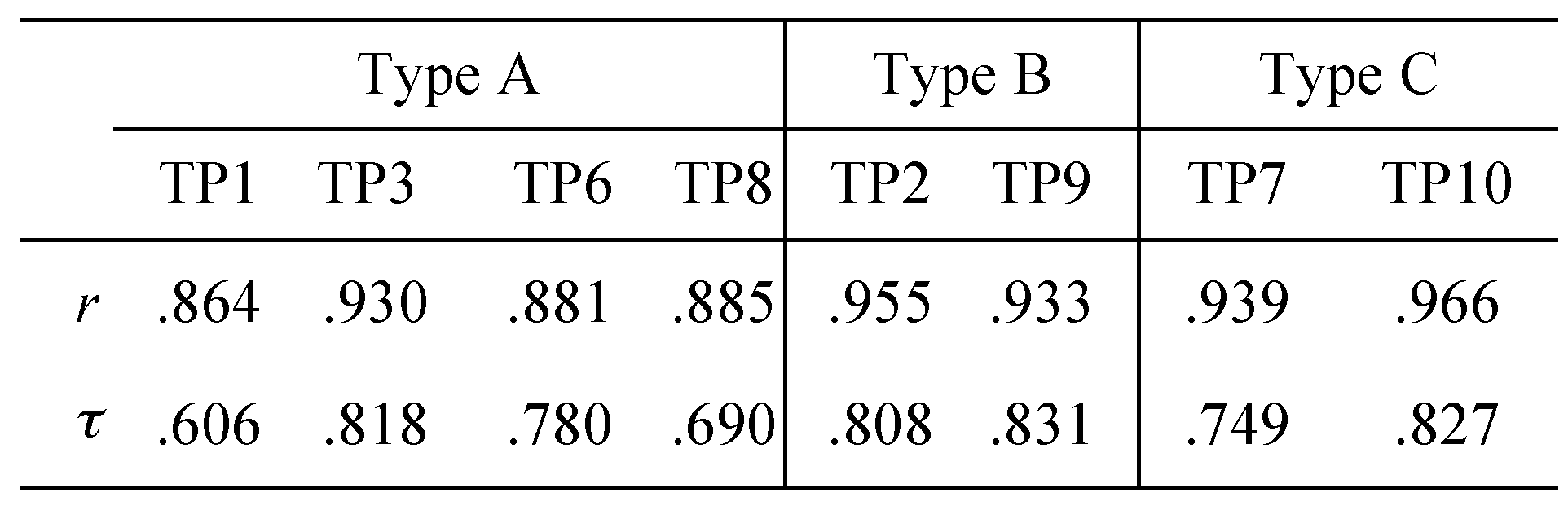
The correlations between NFix and NLop were quite high across TP's, as measured by Pearson's product-moment coefficient shown in

Table 3. Pearson's (r) and Kendall's (τ) correlation coefficients between two heat measures (NFix and NLop) by TP. 

: .864 < r < .966. However, the correlations in ranks, not in magnitude, were somewhat lower, as measured by Kendall's rank coefficients (.606 < τ < .831).

Concerning the first and second modal (i.e., the two most heated) segments, both NFix and NLop showed interesting consistency. As listed in

Table 4. The first and second modal segments on three fixation-related measures. 

, the modal pairs of TP1 (Type A), 2 and 9 (Type B), and, 7 and 10 (Type C) were exactly identical on the two measures. Exceptions were limited to TP3, 6, and 8 of Type A. Among these, the non-identicality on TP3 arose from the reversed order of the pair {A1, B1}. Their values differed only slightly, particularly in NLop. Even on TP6 and 8, A1 maintained its top modality.

This nearly perfect consistency of the modal segments is noteworthy, suggesting the possibility that the frequent loops contributed to the frequent fixations. This was examined in conjunction with the ratio NLop/NFix listed in Table 4.

The contribution in the strict sense was confirmed in only three cases where the first modal segments on NLop, NFix, and NLop/NFix were the same: A1 of TP6 (Type A) as well as D5 of TP7 and B1 of TP10 (Type C). The contribution was weaker in the cases where the second modal segments agreed: B1 of TP1 (Type A), B2 of TP9 (Type B) and A1 of TP7 (Type C). Of these, TP7 alone firmly confirmed the possibility.

A counter tendency was observed on the remaining five pages, in which nearly half of the NFix's (41.9% to 55.6%) were non-loops: A1 of TP3 and 8 (Type A), A1 of TP2 and C2 of TP9 (Type B), A1 of TP10 (Type C). These segments were modal in NFix and NLop but not in NLop/NFix.

Joint Analysis of Heat Maps and Networks

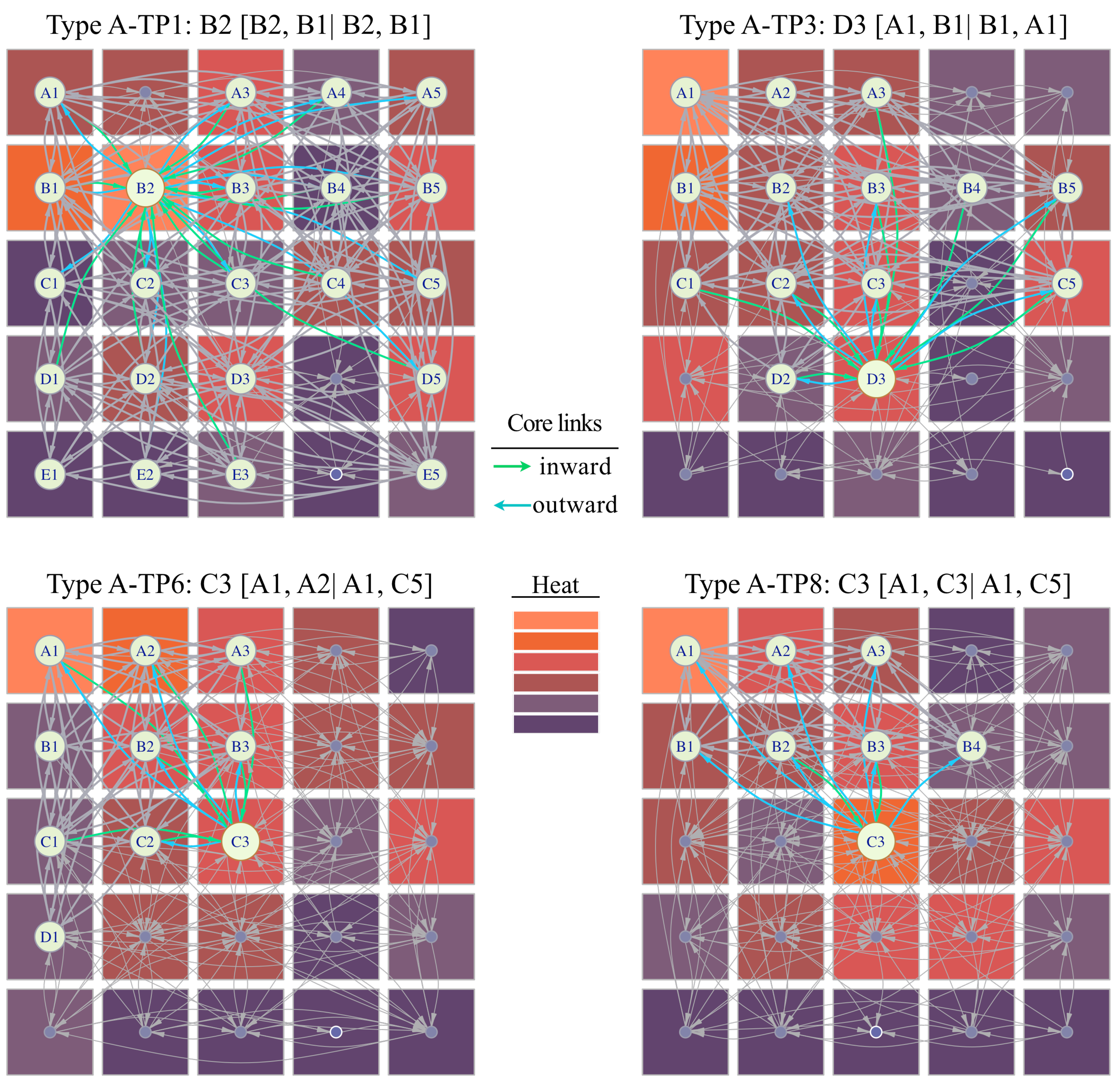
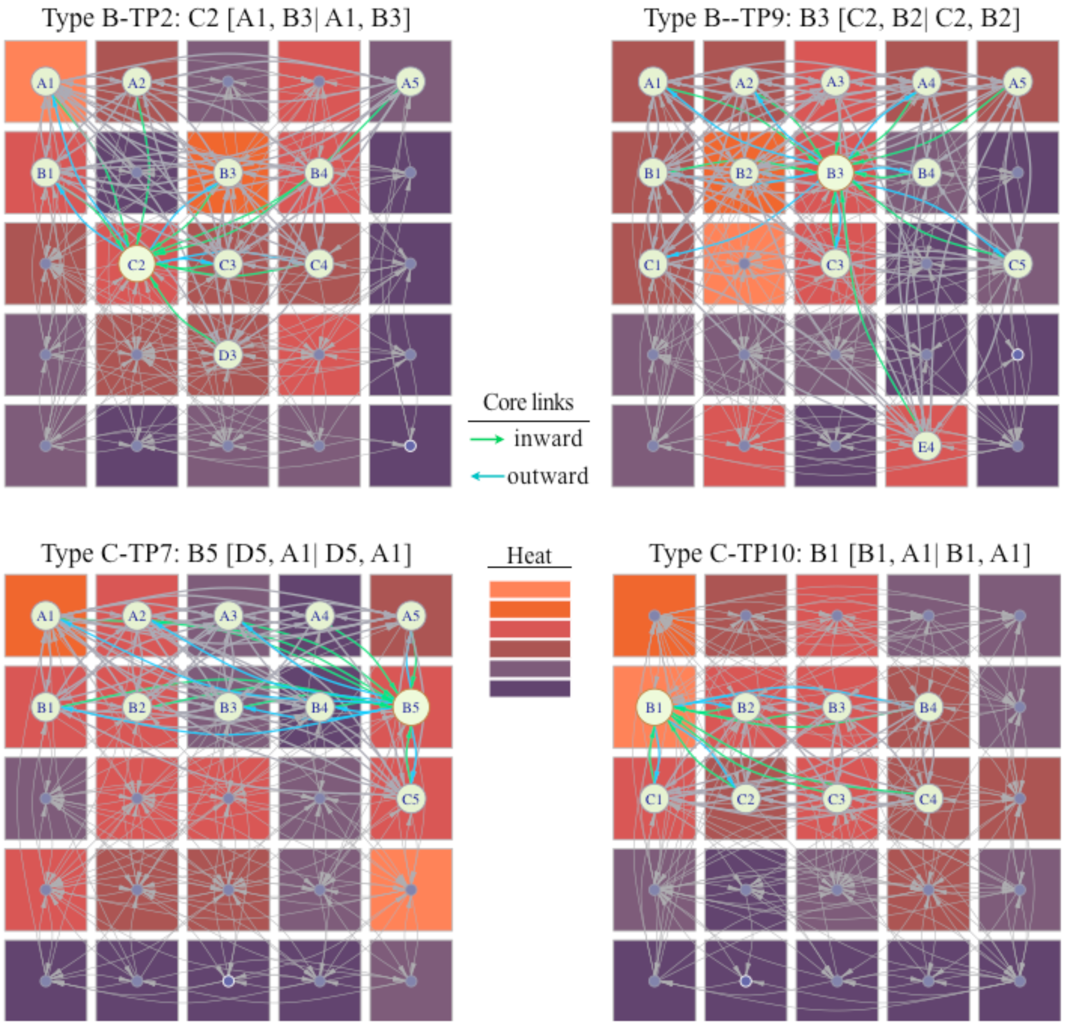
Shown in Figure 5 and Figure 6 are the heat maps by TP overlaid by the respective networks in which the clique-based communities are highlighted by large and bright nodes as well as by segment codes. In addition, the core nodes are the largest in size, while the peripheral nodes, small in size, have light-colored frames. Although most of the nodes are semi-cores and semi-peripherals in the strict sense, they will be called cores and peripherals, respectively, for the sake of brevity, unless particularly necessary.

In these figures, the links connected to (inward) and from (outward) the cores within the individual communities are specially colored using colors different from those used in the previous study (Matsuda et al., 2009, 2011), because of the coloring constrains arising from overlaying.

The heat of the segments of all the core nodes exceeded the 75 percent level, falling in the top three grades. Among them, the primacy of the cores B2 of TP1 (Type A) and B1 of TP10 (Type C) was perfect. These segments were modal in both NFix and NLop, as explained above. However, they differed with respect to NLop/NFix: only C3 maintained the primacy in this ratio. The heat of the other segments fell in the third grade, except for C3 of TP8 (Type A), which belonged to the second grade.

In contrast to the cores, all the peripheral nodes were found in the least heated segments (i.e., grade 6). The lack of importance of the peripherals was also evidenced by the absence of direct links to the cores in the respective networks, except for E3 of TP7 (Type C), which was linked from the core B3. Even this case lacked both static and dynamic importance.

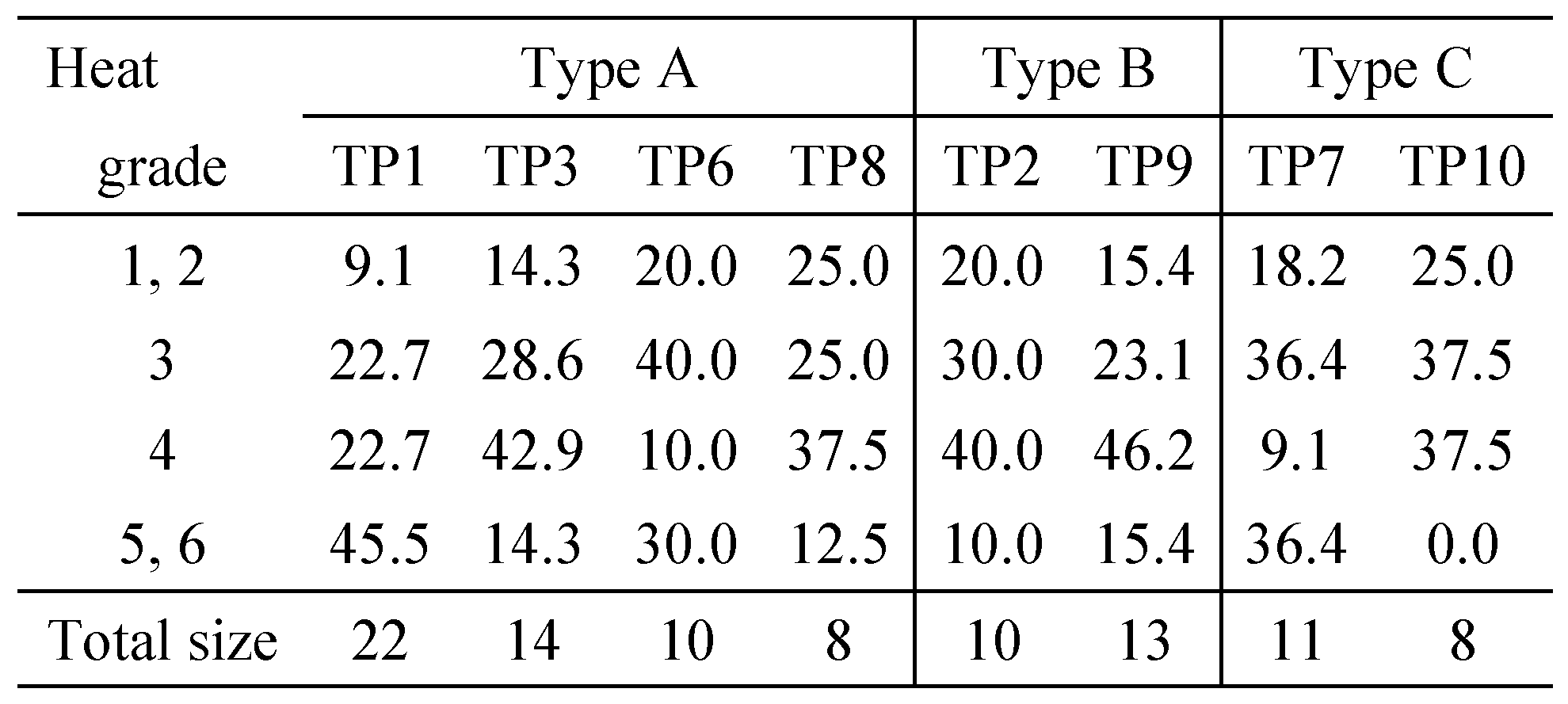
When we extended the scope of importance from the cores to the clique-based community nodes, we found an interesting tendency (see

Table 5. Proportion of the community members by heat grade (%). 

.

). The majority of the community members (>54.5%) were located, on all TP's, in the segments whose heat exceeded the median level (grade 4 or higher). The tendency was more intense on TP6 and 8 (Type A), TP2 (Type B), and TP7 and 10 (Type C): Around 50.0–62.5% of the members belonged to the segments of grade 3 or higher.

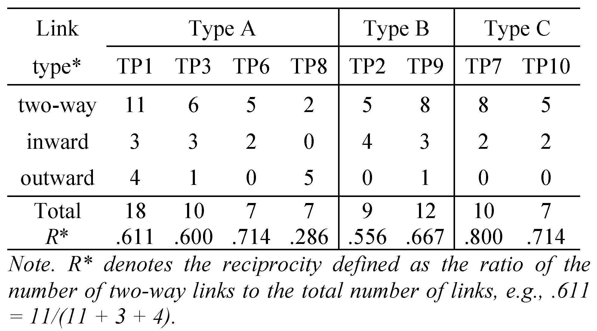
Finally,

Table 6. Number of neighbors of core nodes by type of link. 

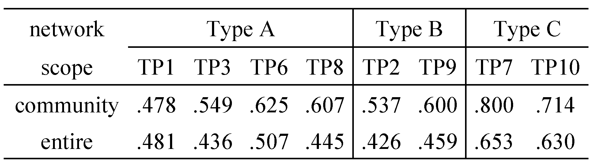
shows the classification of the nodes that were directly connected with the cores by link type: two-way (both inward and outward), inward only, and outward only. As indicated by reciprocity (R*), most of the nodes had two-way links with the respective cores, except for TP8, where outward links were dominant. Generally, the reciprocity tended to increase as we narrowed the scope from entire networks to communities and then to core neighborhoods (see

Table 7. Reciprocity of communities and entire networks. 

).

Discussion

Given a set of coded eye-fixation sequences, researchers can infer two types of importance of each segment: one from the counts of the codes (non-relational), and the other from the transitional relations via the adjacency matrix (see Appendix A). Because the two types of importance are complementary (static and dynamic), their joint analysis is desirable to gain rich knowledge.

The present study revealed an interesting congruence between the static and dynamic importance, namely, in the locations of the most (or least) heated segments and the core (or peripheral) nodes identified in the networks. The core nodes, the most important nodes, were located in the hot segments (whose heat exceeded the 75th percentile level). The opposite congruence was more thorough: the peripheral nodes, the least important nodes, were located in the least heated segments.

Beyond the node-segment matches, extended congruence was observed among the nodes of the clique-based communities bearing importance in terms of fairly tight connections to the cores. The majority of the clique-based community members were in the warm to hot segments (whose heat exceeded the 50th percentile level, i.e., the median).

Considering the fact that the centrality indices incorporate the presence of relations (i.e., transitions) but not their magnitudes, the observed congruence between the frequency-based heat maps and the network nodes was unexpectedly high. The results confirm the merit of the present approach, but there is room for further investigation.

In addition to the congruence, we found that the proportion of the two-way links, as measured by reciprocity, tended to increase as the scope of analysis was narrowed from entire networks to communities and then to core neighborhoods.

A note has been made in the previous section about the prominent primacy of the two cores located in the most heated segments: B2 of TP1 (Type A) and B1 of TP10 (Type C). Upon close examination, we found that the former was the sole genuine core being ranked highest on all six indices. The latter was a semi-core in the strict sense, being ranked highest in four out of six indices: degree, closeness, PageRank, and authority. D3 of TP3 (Type A) also had four top rankings, but the heat of the corresponding segment was not in the top two grades. The two semi-cores (B1-TP10-C, D3-TP3-A for short) ranked highest in degree, closeness, and PageRank, but they differed in the other indices: Their rankings in <betweenness, authority-, hub-scores> were <7, 1, 8> on B1-TP10-C and <1, 2, 6> on D3-TP3-A. If they differed solely in the centrality indices or the ranking scores, the explanation would be far less complicated. A clue to the answer may lie in the large difference in the betweenness scores and the minor differences in the authority- and hub-scores. As explained in brief in Introduction, betweenness reflects the global structure, but currently available algorithms disregard the link weights. Authority- and hub-scores also reflect the global structure, but they incorporate the weights. Hence, for further analysis, we need to wait for the completion of the algorithm for weighted betweenness.

The observed relationships between the fixations (NFix) and the loops (NLop) are also noteworthy, since they indicate recurrent and sustained attention. The use of the ratio NLop/NFix helped us separate three cases in which the large NLops contributed to the large NFixs: A1-TP6-A, D5-TP7-C and B1-TP10-C. Moreover, in five out of the remaining seven cases, we found the counter tendency, namely, nearly half of the large NFix's resulted from non-loops: A1-TP3-A, A1-TP8-A, A1-TP2-B, C2-TP9-B and A1-TP10-C. These results motivated us to investigate patterns of shifts beyond pairs of segments, as recorded in the adjacency matrices.

Although the present approach has merits, it has a limitation arising from the potential dominance of one or a few records in the aggregate tendencies. For instance, a very hot segment may result from a large number of fixations concentrated in a limited number of records (Naturally, unattended segments are free from such a possibility). Similarly, transitions in an adjacency matrix may be dominated by the particular tendency of a few records. This in turn will influence the computation of the ranking scores.

This limitation may be overcome by looking for patterns shared among records. Furthermore, if we explore sequential patterns, we would be able to extend the span of dynamic relationships beyond the chains of node pairs to longer sequences. Suppose links A2-B1 and B1-C4 (in the present coding system) are identified in network analysis, it would be difficult to know whether they resulted from the triad sequence A2-B1-C4 frequently shared among records.

We expect the concept of PrefixSpan (Pei et al., 2001) for frequent pattern mining and Graph Mining (see Chakarabarti et al., 2006) to lead us to extract motifs, i.e., the basic sequence of transitions. The output of this line of search can be used to test the generality of the scan patterns, such as F-shaped (Nielsen, 2006; Nielsen et al., 2010), zigzag (Lorigo et al., 2008), and Z-shaped (as believed by many leaflet designers) patterns.

Probably, many practitioners and students have been inspired by Nielsen and Pernice's (2010) book, which includes viewing patterns of individuals on various web pages. Nielsen and Pernice employed both pixel-based heat maps and gaze plots based on fixation duration rather than frequencies. Their gaze plot is actually a scan path augmented by dots (circles) varying in size according to the fixation duration. However, the overlapping dots make it hard to discern the heat of the dots and trace the trajectory that is frequently covered by the dots. More importantly, the transitional importance is not considered. It is clear that those who are interested in single-case studies can benefit from applying our approach, which enables the quantification of importance and the examination of closely linked segments such as communities and neighborhoods.

Finally, we point out that the identification of the core nodes should be guided by the research purpose and not restricted to the congruence of several indices. For instance, one can use the centrality degree alone or in combination with closeness, if node-centric importance is pertinent. In contrast, betweenness is useful if one is concerned with the mediating importance in the flow of attention over the entire network. Alternatively, one can employ PageRank and/or authority- and hub-scores if one focuses on recursive rankings.