The Influence of Eye Model Parameter Variations on Simulated Eye-Tracking Outcomes
Abstract
:Introduction
Methods
Comparative Studies
Stochastic Eye Model

Simulation Procedure
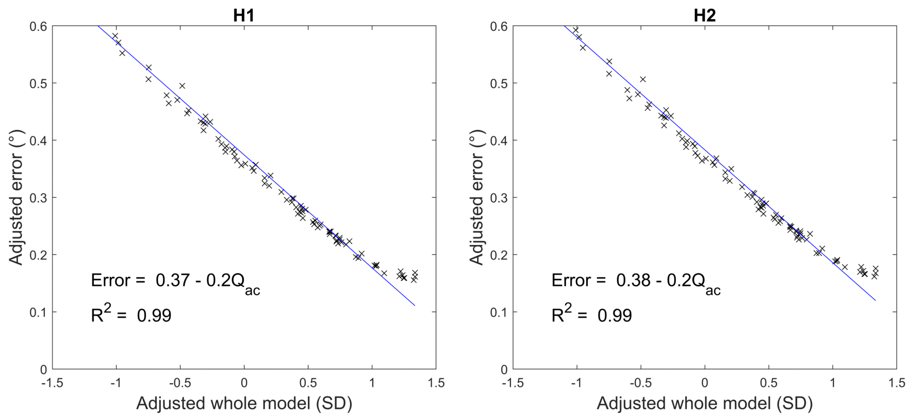
Analyses

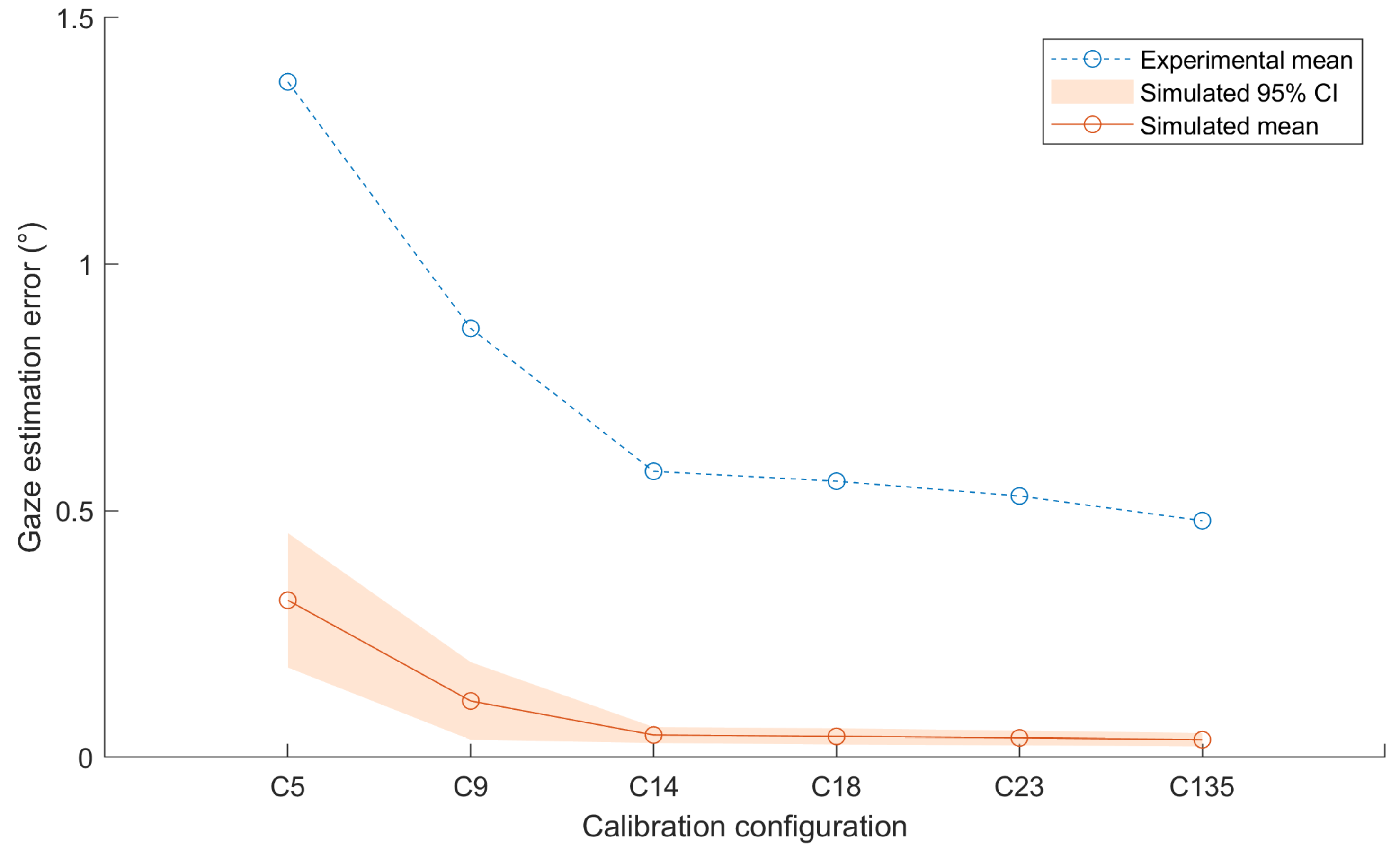
Results
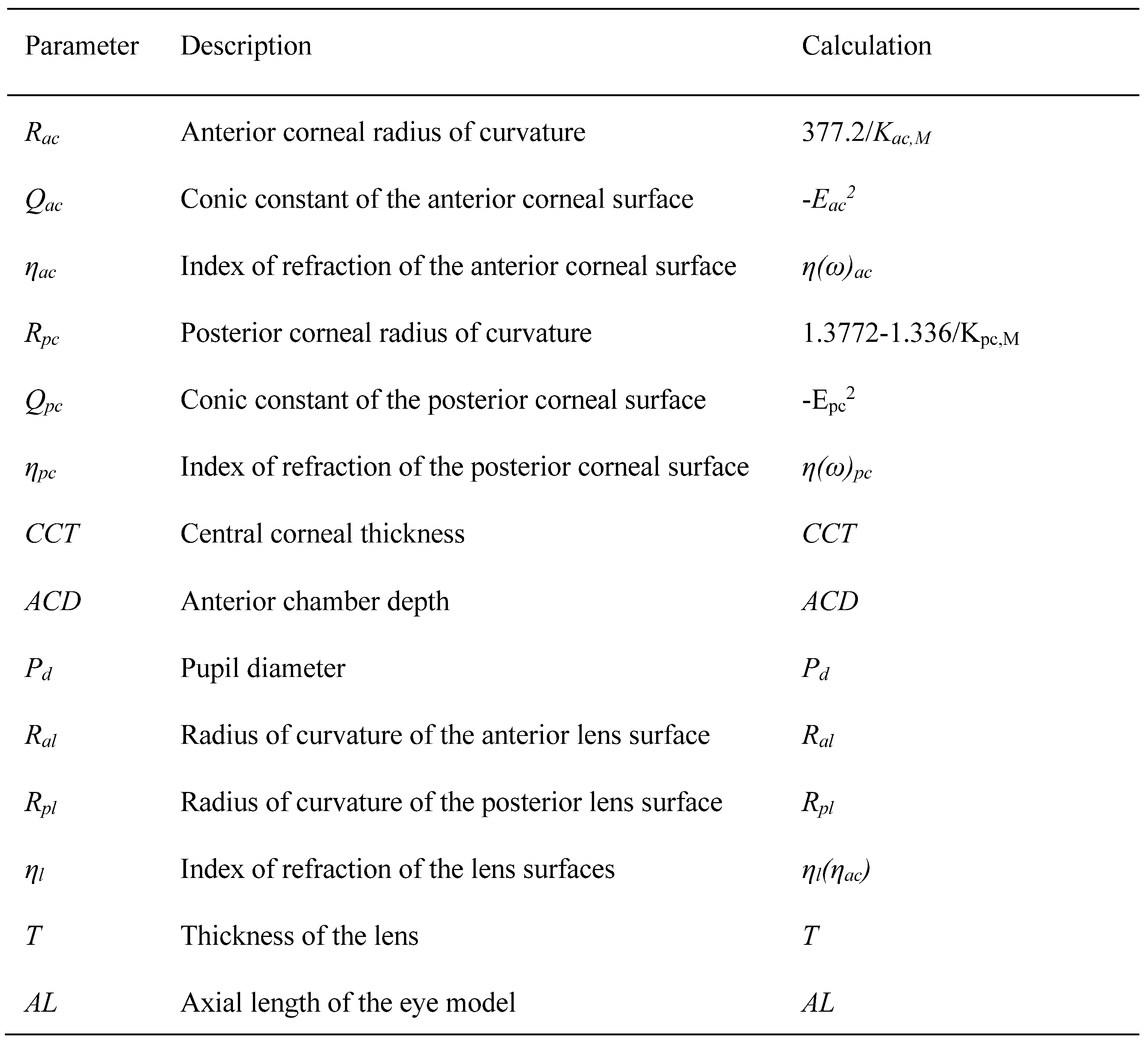
Eye Model Parameters
Simulated Image Features
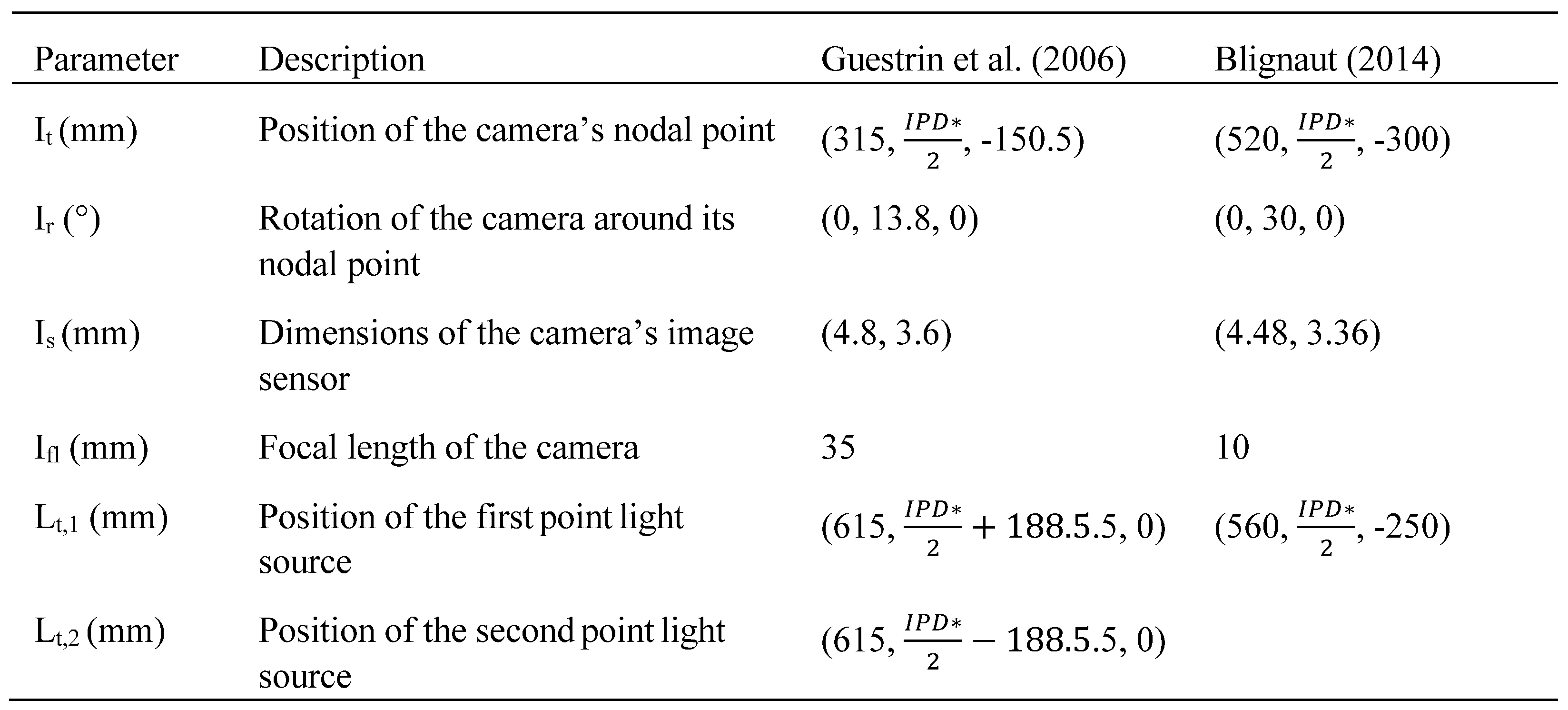
Guestrin and Eizenman (2006)
Blignaut (2014)
Discussion
Implications of Findings
Limitations
Future Work
Ethics and Conflict of Interest
Acknowledgments
References
- Aguirre, G. K. 2019. A model of the entrance pupil of the human eye. Scientific reports 9, 1: 9360. [Google Scholar] [CrossRef] [PubMed]
- Atchison, D. A., and G. Smith. 2005. Chromatic dispersions of the ocular media of human eyes. Journal of the Optical Society of America A 22, 1: 29–37. [Google Scholar]
- Atchison, D. A. 2006. Optical models for human myopic eyes. Vision research 46, 14: 2236–2250. [Google Scholar] [CrossRef]
- Bergmanson, J., A. Burns, and M. Walker. 2019. Anatomical explanation for the central-peripheral thickness difference in human corneas. Investigative Ophthalmology & Visual Science 60, 9: 4652–4652. [Google Scholar]
- Blignaut, P., and D. Wium. 2013. The effect of mapping function on the accuracy of a video-based eye tracker. Proceedings of the 2013 conference on eye tracking South Africa; pp. 39–46. [Google Scholar] [CrossRef]
- Blignaut, P. 2014. Mapping the pupil-glint vector to gaze coordinates in a simple video-based eye tracker. Journal of Eye Movement Research 7, 1. [Google Scholar] [CrossRef]
- Blignaut, P. 2016. Idiosyncratic feature-based gaze mapping. Journal of Eye Movement Research 9, 3. [Google Scholar] [CrossRef]
- Böhme, M., M. Dorr, M. Graw, T. Martinetz, and E. Barth. 2008. A software framework for simulating eye trackers. Proceedings of the 2008 symposium on Eye tracking research & applications; pp. 251–258. [Google Scholar] [CrossRef]
- Choe, K. W., R. Blake, and S. H. Lee. 2016. Pupil size dynamics during fixation impact the accuracy and precision of video-based gaze estimation. Vision research 118: 48–59. [Google Scholar]
- Dierkes, K., M. Kassner, and A. Bulling. 2018. A novel approach to single camera, glintfree 3D eye model fitting including corneal refraction. Proceedings of the 2018 ACM Symposium on Eye Tracking Research & Applications, June; pp. 1–9. [Google Scholar] [CrossRef]
- Dodgson, N. A. 2004. Variation and extrema of human interpupillary distance. Stereoscopic displays and virtual reality systems XI, May, vol. 5291, pp. 36–46. [Google Scholar] [CrossRef]
- Draper, N. R., and H. Smith. 1998. Applied regression analysis, 326. [Google Scholar]
- Durr, G. M., E. Auvinet, J. Ong, J. Meunier, and I. Brunette. 2015. Corneal shape, volume, and interocular symmetry: parameters to optimize the design of biosynthetic corneal substitutes. Investigative Ophthalmology & Visual Science 56, 8: 4275–4282. [Google Scholar] [CrossRef]
- Guestrin, E. D., and M. Eizenman. 2006. General theory of remote gaze estimation using the pupil center and corneal reflections. IEEE Transactions on biomedical engineering 53, 6: 1124–1133. [Google Scholar] [CrossRef]
- Hansen, D. W., J. S. Agustin, and A. Villanueva. 2010. Homography normalization for robust gaze estimation in uncalibrated setups. Proceedings of the 2010 symposium on eye-tracking research & applications; pp. 13–20. [Google Scholar] [CrossRef]
- Holmqvist, K. 2017. Common predictors of accuracy, precision and data loss in 12 eye-trackers. In The 7th Scandinavian Workshop on Eye Tracking. pp. 1–25. [Google Scholar] [CrossRef]
- Huang, J. B., Q. Cai, Z. Liu, N. Ahuja, and Z. Zhang. 2014. Towards accurate and robust crossratio based gaze trackers through learning from simulation. Proceedings of the Symposium on Eye Tracking Research and Applications; pp. 75–82. [Google Scholar] [CrossRef]
- Kar, A., and P. Corcoran. 2017. A review and analysis of eye-gaze estimation systems, algorithms and performance evaluation methods in consumer platforms. IEEE Access 5: 16495–16519. Available online: https://ieeexplore.ieee.org/document/8003267.
- Kim, J., M. Stengel, A. Majercik, S. De Mello, D. Dunn, S. Laine, M. McGuire, and D. Luebke. 2019. Nvgaze: An anatomically-informed dataset for low-latency, near-eye gaze estimation. Proceedings of the 2019 CHI conference on human factors in computing systems; pp. 1–12. [Google Scholar] [CrossRef]
- Lai, C.C., S.W. Shih, and Y.P. Hung. 2014. Hybrid method for 3-D gaze tracking using glint and contour features. IEEE Transactions on Circuits and Systems for Video Technology 25, 1: 2437. [Google Scholar] [CrossRef]
- Mardanbegi, D., and D. W. Hansen. 2012. Parallax error in the monocular headmounted eye trackers. Proceedings of the 2012 acm conference on ubiquitous computing, September; pp. 689–694. [Google Scholar] [CrossRef]
- Nair, N., R. Kothari, A. K. Chaudhary, Z. Yang, G. J. Diaz, J. B. Pelz, and R. J. Bailey. 2020. RIT-Eyes: Rendering of near-eye images for eye-tracking applications. ACM Symposium on Applied Perception 2020, September; pp. 1–9. [Google Scholar] [CrossRef]
- Narcizo, F. B., F. E. D. Dos Santos, and D. W. Hansen. 2021. High-accuracy gaze estimation for interpolation-based eye-tracking methods. Vision 5, 3: 41. [Google Scholar] [CrossRef] [PubMed]
- Nowakowski, M., M. Sheehan, D. Neal, and A. V. Goncharov. 2012. Investigation of the isoplanatic patch and wavefront aberration along the pupillary axis compared to the line of sight in the eye. Biomedical optics express 3, 2: 240–258. [Google Scholar] [CrossRef]
- Petersch, B., and K. Dierkes. 2022. Gaze-angle dependency of pupil-size measurements in headmounted eye tracking. Behavior Research Methods 54, 2: 763–779. [Google Scholar] [CrossRef] [PubMed]
- Polans, J., B. Jaeken, R. P. McNabb, P. Artal, and J. A. Izatt. 2015. Wide-field optical model of the human eye with asymmetrically tilted and decentered lens that reproduces measured ocular aberrations. Optica 2, 2: 124–134. [Google Scholar] [CrossRef]
- Porta, S., B. Bossavit, R. Cabeza, A. Larumbe-Bergera, G. Garde, and A. Villanueva. 2019. U2Eyes: A binocular dataset for eye tracking and gaze estimation. Proceedings of the IEEE/CVF International Conference on Computer Vision Workshops; pp. 3660–3664. [Google Scholar]
- Rozema, J. J., D. A. Atchison, and M. J. Tassignon. 2011. Statistical eye model for normal eyes. Investigative Ophthalmology & Visual Science 52, 7: 4525–4533. [Google Scholar] [CrossRef]
- Rozema, J. J., P. Rodriguez, R. Navarro, and M. J. Tassignon. 2016. SyntEyes: a higher-order statistical eye model for healthy eyes. Investigative ophthalmology & visual science 57, 2: 683–691. [Google Scholar] [CrossRef]
- Świrski, L., and N. Dodgson. 2014. Rendering synthetic ground truth images for eye tracker evaluation. Proceedings of the Symposium on Eye Tracking Research and Applications; pp. 219–222. [Google Scholar] [CrossRef]
- Szczęsna, D. H., and H. T. Kasprzak. 2006. The modelling of the influence of a corneal geometry on the pupil image of the human eye. Optik 117, 7: 341–347. [Google Scholar] [CrossRef]
- Wood, E., T. Baltrušaitis, L. P. Morency, P. Robinson, and A. Bulling. 2016. Learning an appearance-based gaze estimator from one million synthesised images. Proceedings of the Ninth Biennial ACM Symposium on Eye Tracking Research & Applications; pp. 131–138. [Google Scholar] [CrossRef]
- Villanueva, A., and R. Cabeza. 2008. A novel gaze estimation system with one calibration point. IEEE Transactions on Systems, Man, and Cybernetics, Part B (Cybernetics) 38, 4: 1123–1138. [Google Scholar] [CrossRef] [PubMed]
- Wood, E., T. Baltrušaitis, L. P. Morency, P. Robinson, and A. Bulling. 2016. Learning an appearance-based gaze estimator from one million synthesised images. Proceedings of the Ninth Biennial ACM Symposium on Eye Tracking Research & Applications, March; pp. 131–138. [Google Scholar] [CrossRef]
- Velleman, P. F., and R. E. Welsch. 1981. Efficient computing of regression diagnostics. The American Statistician 35, 4: 234–242. Available online: https://10.1080/00031305.1981.10479362. [CrossRef]


 |
 |
 |
 |
 |
Copyright © 2023. This article is licensed under a Creative Commons Attribution 4.0 International License.
Share and Cite
Fischer, J.; van der Merwe, J.; Vandenheever, D. The Influence of Eye Model Parameter Variations on Simulated Eye-Tracking Outcomes. J. Eye Mov. Res. 2023, 16, 1-17. https://doi.org/10.16910/jemr.16.3.1
Fischer J, van der Merwe J, Vandenheever D. The Influence of Eye Model Parameter Variations on Simulated Eye-Tracking Outcomes. Journal of Eye Movement Research. 2023; 16(3):1-17. https://doi.org/10.16910/jemr.16.3.1
Chicago/Turabian StyleFischer, Joshua, Johan van der Merwe, and David Vandenheever. 2023. "The Influence of Eye Model Parameter Variations on Simulated Eye-Tracking Outcomes" Journal of Eye Movement Research 16, no. 3: 1-17. https://doi.org/10.16910/jemr.16.3.1
APA StyleFischer, J., van der Merwe, J., & Vandenheever, D. (2023). The Influence of Eye Model Parameter Variations on Simulated Eye-Tracking Outcomes. Journal of Eye Movement Research, 16(3), 1-17. https://doi.org/10.16910/jemr.16.3.1