Forecasting Detrended Volatility Risk and Financial Price Series Using LSTM Neural Networks and XGBoost Regressor

Abstract

It is common practice to employ returns, price differences or log returns for financial risk estimation and time series forecasting. In De Prado’s 2018 book, it was argued that by using returns we lose memory of time series. In order to verify this statement, we examined the differences between fractional differencing and logarithmic transformations and their impact on data memory. We employed LSTM (long short-term memory) recurrent neural networks and an XGBoost regressor on the data using those transformations. We forecasted risk (volatility) and price value and compared the results of all models using original, unmodified prices. From the results, models showed that, on average, a logarithmic transformation achieved better volatility predictions in terms of mean squared error and accuracy. Logarithmic transformation was the most promising transformation in terms of profitability. Our results were controversial to Marco Lopez de Prado’s suggestion, as we managed to achieve the most accurate volatility predictions in terms of mean squared error and accuracy using logarithmic transformation instead of fractional differencing. This transformation was also most promising in terms of profitability.

1. Introduction

It is common practice to make statistical measures of time series invariant over time to describe data points more precisely using traditional regression methods. Moreover, various data transformations affect how much memory or similarity will remain between modified and unmodified series. However, it is unknown how important data transformation and correlation is to the original form and how they can affect the accuracy of predictions in machine learning. In this research, we compare how well recurrent neural networks perform with and without different data transformations in terms of forecasting prices and volatility, which will be evaluated using different metrics. We will also look into the accuracy of next-day prediction, create a strategy by using different strategies and seek to maximize our profit. These metrics will be the main criteria to determine how well the recurrent neural networks can be applied in daily trading.

To understand detrending (making time series stationary), we have to understand the reasoning for that and how transformation affects time series. In general, we detrend time series to make their mean, variance, and autocorrelation constant over time or, in other words, to decompose them into parts and remove their trend and seasonality components. Removing these parts makes time series more suitable for linear regression, where linear models such as ARIMA benefit the most (more discussed by Millionis (2004)). In general, this implies that the relationship between previous data points and the following ones holds the same relationship; thus, they perform poorly on long-term forecasting because they strongly depend on previous values. On the contrary, we have recurrent neural networks, which are not dependent on a condition for linearity to be satisfied. The best example would be LSTM cells, which excel at remembering long-term dependencies, meaning that with sufficient training data, they can determine the changing fluctuations of the time series.

Like any other model, RNNs are susceptible to a sudden change in financial market behavior. If you train your model using time series when the market was under the influence of certain properties, your testing set can differ from reality if new externalities occur that drastically reshape how the market acts without any similarity in the past. This can also take some time for the model to relearn. However, if a detrended time series were used, then despite the drastic change, the model will likely have better results since it is easier to learn stationary data, or at the very least, use inverse transformation to apply previous day information to have a more accurate prediction. This is also suggested by Salles et al. (2019) in “Non-stationary time series transformation methods: An experimental review”, where the author concludes that to obtain more accurate results, time series transformations in machine learning are necessary.

2. Fractional Differencing for Stationarity and Memory

In “Advances in financial machine learning” de Prado (2018), the author justifies the loss of memory in a time series by examining the relation between non-stationary time series and its stationary transformation, specifically by comparing using first-order logarithmic and fractional differencing usually used for long memory analysis Carreno Jara (2011), Maynard et al. (2013), Sadaei et al. (2016), Baillie (1996). To fully understand this, we have to look into the fractional differentiation of order d:

$$X_t=d{X}_{t-1}-\frac{d(d-1)}{2!}{X}_{t-2}+\frac{d(d-1)(d-2)}{3!}{X}_{t-3}-\dots +{ϵ}_t$$

and rewrite it for our time series ${\left\{S_t\right\}}_{t=1,\dots ,T}$ at time t with weights; then, we obtain its transformation

$$\widehat{S_t}=\sum _{k=0}^{\infty }{\omega }_k{S}_{t-k}$$

with

$${\omega }_0=1\mathrm{and}{\omega }_k=-{\omega }_{k-1}\frac{d-k+1}{k}.$$

Given $d\in (0,1)$, all weights after ${\omega }_0=1$ will be negative and greater than $-1$. When $d=0$, all weights are 0 except for ${\omega }_0=1$, and when $d=1$, we have a standard first-order differentiation because weights sequence $\left\{{\omega }_k\right\}=\{1,-1,0\dots \}$.

In his book de Prado (2018), de Prado provides an example of E-mini S&P log-prices, where the statistic of the Augmented Dickey–Fuller test with $d=0$ (original time series) is $=-0.3387$ and $-3.2733$ with $d=0.4$, while the critical value of 5% is $-2.8623$, meaning that the null hypothesis of the unit root can be rejected after fractional differentiation transformation. Furthermore, the correlation between the two datasets (original and transformed) is around $0.995$, indicating that the memory is still preserved. In comparison, a transformation with $d=1$ gives an ADF statistic of $-46.9114$, but correlation with the original set falls to 0.05. Thus, to achieve stationarity, it is sufficient to fractionally differentiate.

It is easy to see that weights are a recursive sequence that is decreasing and bounded. This means that is has limit $L={lim}_{k\to \infty }{\omega }_k$, and we can show that $L={lim}_{k\to \infty }{\omega }_k=-{lim}_{k\to \infty }{\omega }_{k-1}\frac{d-k+1}{k}=-L*{lim}_{k\to \infty }\frac{d-k+1}{k}(\sin \mathrm{ce}\mathrm{both}\mathrm{limits}\mathrm{exist})=-L*1=-L$. By solving equation $L=-L$, we obtain $L=0$. This can also be seen from Figure 1, as k increases, the weights converge to zero; in other words, the present time variable dependence on historical values decreases and memory fades.

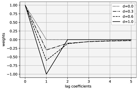
Figure 1. Weights distributed to different lag coefficients.

Memory in Time Series

There are a lot of debates in the financial world about the stationary vs. memory dilemma. Some argue that these two concepts have no correlation Kom Samo (2018) as there are too many assumptions to be considered, while others oppose that opinion. Upon further reading, we tried to evaluate memory in time series before and after fractional differencing from a practitioner’s perspective.

The transformation of fractional differentiation is based on the idea that by transforming present values in relation to past values, the data series persist its trend. This implies that there is a significant connection between trends of original and transformed time series or that there is a correlation between those two sets.

In Figure 2, autocorrelations of fractionally different time series take some time to completely disappear, indicating longer memory compared to first-order difference of logarithmic time series where previous values have no significant relation to each other.

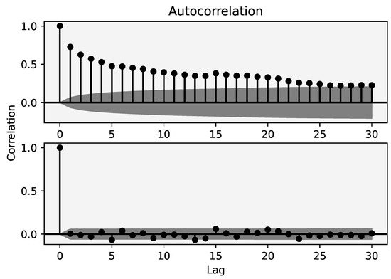
Figure 2. Autocorrelation functions of time series transformation with d = opt (upper one) and d = 1 (lower one).

Hosking (1981) proposed that fractionally differenced processes exhibit long-term persistence and anti-persistence. One way to examine the persistence of time series is to use the Hurst exponent. The Hurst exponent H ranges between 0 and 1. If value $0<H<0.5$, it implies an anti-persistent series, meaning that any positive movement will likely be followed by a negative step and vice versa. If value $0.5<H<1$, it implies that any positive/negative change in time steps will be followed accordingly by positive/negative change. A value of $H=0.5$ indicates no correlation between a series variable and its past values. Since the Hurst exponent relates to the autocorrelations lag rate changes, we can further calculate the decrease in the Hurst exponent and time series trend. An important note is that after adapting the rescaled range analysis, we calculated the average Hurst exponent of all future contracts volatility and prices being on average at around $0.602$ and $0.449$, respectively, indicating that the series of volatility consists of persistence, while prices consist of anti-persistence as well as lack of long memory in time series and the rapid decay of correlations in time. In theory, cases with short memory use ARIMA models as they are more suitable compared to ARFIMA (ARIMA with a fractionally differenced lag), which is used to represent long-range time series.

3. Methodology

In this research, we used 22 future contract close prices as our data. Out of those 22 symbols, 5 were from agricultural, 5 from currency, 5 from the interest rate, 3 from metal, 2 from stock, and 2 from energy sectors. Below, we present a brief description of each of the following experiments:

• Forecasting true range volatility with RNN;
• Forecasting close prices with RNN and implementing results with two strategies;
• Forecasting close prices with XGBoost regressor and implementing results with two strategies.

Each of the experiments was performed for three different time series transformations:

I.

Unmodified time series, without any manipulation, noted as d = 0;

II.

Fractional differenced time series with minimal order d to pass ADF test, noted as d = opt;

III.

Classical logarithmic transformation, noted as d = 1.

Implemented strategies We will be using two simple algorithmic trading strategies. The first strategy uses next-day predictions to determine new positions—if next-day prediction is higher (or lower) than our previous prediction, then the position will be 1 or $-1$ (long or short). The second strategy is more intuitive; if the prediction is higher than today’s price, we will go long, and if the prediction is lower, we will go short. Let us denote our strategy $H_t$, $S_t$ as real price and ${\widehat{S}}_t$ as predicted price, where t indicates time. When our strategies can be described as:

$$\mathrm{Strategy}\mathrm{no}.1:H_t=1\mathrm{if}{\widehat{S}}_t<{\widehat{S}}_{t+1};H_t=-1,\mathrm{if}{\widehat{S}}_t>{\widehat{S}}_{t+1};$$

$$\mathrm{Strategy}\mathrm{no}.2:H_t=1\mathrm{if}{S}_t<{\widehat{S}}_{t+1};H_t=-1,\mathrm{if}{S}_t>{\widehat{S}}_{t+1}.$$

The reason to implement strategy no.1 is that in some cases, RNN can manage to minimize loss efficiently despite the fact that its prediction is below or above our target. However, we can still try to see how accurate predicted positions are.

Data Transformations

In Figure 3 and Figure 4, we will show a process of detrending a few selected symbols. Before any transformation, time series were randomly distributed Figure 4, indicating non-stationarity.

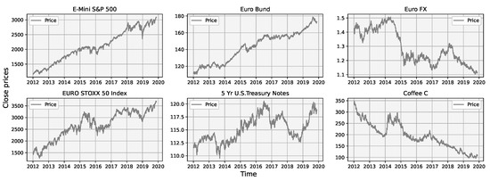
Figure 3. Non-stationary prices of selected futures during an 8 year period.

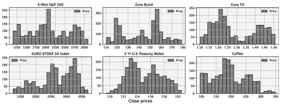
Figure 4. Distribution of selected non-stationary futures prices during an 8 year period.

After the transformation to stationary prices, we can visually see the drastic change in their distributions in Figure 5 and Figure 6.

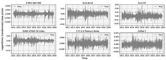
Figure 5. Selected futures prices after logarithmic transformation during an 8 year period.

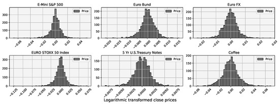
Figure 6. Distribution of selected futures logarithmic returns during 8 year period.

To confirm stationarity, we applied the ADF test to check if there is a need for second-order differentiation as well as a measured correlation between the original set and transformed, see Table 1. Critical value being $-2.863$ at the 95% confidence level.

Table 1. First-order logarithmic differenced series ADF test results and correlation with original series.

Symbol	ADF Statistic	Correlation
ES	$-22.480$	0.001908
FESX	$-8.815$	0.014000
FGBL	$-46.013$	0.002109
FV	$-21.003$	0.042371
KC	$-31.127$	0.017448
EC	$-46.760$	0.030828

According to de Prado (2018), all future contracts achieve stationarity at around $d<0.6$, and most of them are stationary even at $d<0.3$. We conducted the same experiment on 22 futures contracts, and all of them proved Marcos Lopez de Prado’s statement, passing the ADF test with $d<0.6$, and a part of them achieved stationarity with $d=0.3$. Furthermore, looking into those symbols that passed the ADF test, the average correlation between original and transformed data sets with $d=0.6$ is equal to 0.381 and with $d=0.3$ to $0.784$, indicating that the time series with $d=0.6$ might be over-differentiated, removing unnecessary information to achieve stationarity. The results of selected symbols statistics after fractional differencing are seen in Table 2.

Table 2. Statistics of fractional differenced series ADF test results and correlation with original series.

Symbol	ADF Statistic	Correlation
ES	$-7.143408$	0.749509
FESX	$-5.202948$	$-0.182082$
FGBL	$-7.339610$	0.787414
FV	$-7.850287$	0.724982
KC	$-4.875684$	$-0.310578$
EC	$-7.144471$	0.893624

Evaluation metrics

For prediction evaluation, we are using three metrics.

• Profitability. We integrate predictions into the two strategies mentioned above to simulate how profitable each of them could be.
• Accuracy. Position accuracy calculates how many times our predictions from ${\widehat{S}}_t$ to ${\widehat{S}}_{t+1}$ will go in the same direction as the real price movement from $S_t$ to $S_{t+1}$.

  $$\mathit{Accuracy}=\frac{1}{n-1}\sum _{t=1}^{\infty }{𝟙}_{\{sgn(S_{t+1}-S_t)=sgn({\widehat{S}}_{t+1}-{\widehat{S}}_t)\}}.$$
• MSE. Third metric mean squared error, which calculates how far the distance is from the true values of the time series to our estimated regression

  $$\mathit{MSE}=\frac{1}{n}\sum _{t=1}^n(S_t-{\widehat{S}}_t).$$

The experiment was conducted with Python using the Keras library. Because of time consumption, we grouped similarly correlated time series and predicted each group with different models. The hyperparameters for models were selected using the tryout approach. The Adam optimizer was used for all models with MSE as our loss function.

The dataset of each symbol was divided into 3 parts: training, validation, and test samples with the following ratio: 5:1:1 varying from January of 2012 until November of 2019. To deal with underfitting, we monitored each symbol’s performance by looking at the training and validation loss graph, which indicates if there is room for improvement. We also implemented early stopping to stop the model at the inflection point in validation loss to prevent overfitting.

4. Results

Forecasting risk (volatility) using True Range

Table 3 shows the tabulated results of machine learning forecasted volatility using different time series transformations. We used accuracy and MSE for measuring predictions (Figure 7).

Table 3. Accuracy and MSE results of predicted true range volatility.

Symbol	Accuracy			MSE
	d = 0	d = opt	d = 1	d = 0	d = opt	d = 1
BP	0.59	0.61	0.61	$\mathbf{1.12}\times {\mathbf{10}}^{-\mathbf{7}}$	$1.25\times {10}^{-7}$	$1.16\times {10}^{-7}$
C	0.43	0.60	0.51	$7.21\times {10}^{-4}$	$1.38\times {10}^{-2}$	$\mathbf{6.09}\times {\mathbf{10}}^{-\mathbf{4}}$
SB	0.56	0.59	0.59	$1.89\times {10}^{-4}$	$5.90\times {10}^{-5}$	$\mathbf{3.66}\times {\mathbf{10}}^{-\mathbf{5}}$
SI	0.51	0.49	0.48	$1.44\times {10}^{-3}$	$3.06\times {10}^{-4}$	$\mathbf{2.32}\times {\mathbf{10}}^{-\mathbf{4}}$
ES	0.69	0.70	0.70	$\mathbf{2.20}\times {\mathbf{10}}^{-\mathbf{2}}$	$2.21\times {10}^{-2}$	$2.82\times {10}^{-2}$
SF	0.57	0.58	0.58	$4.14\times {10}^{-8}$	$\mathbf{3.16}\times {\mathbf{10}}^{-\mathbf{8}}$	$3.64\times {10}^{-8}$
ED	0.65	0.71	0.65	$1.79\times {10}^{-5}$	$6.84\times {10}^{-3}$	$\mathbf{3.96}\times {\mathbf{10}}^{-\mathbf{6}}$
RR	0.56	0.58	0.62	$3.37\times {10}^{-5}$	$6.22\times {10}^{-5}$	$\mathbf{2.40}\times {\mathbf{10}}^{-\mathbf{5}}$
PL	0.59	0.61	0.72	$1.96\times {10}^{-2}$	$6.02\times {10}^{-3}$	$\mathbf{3.04}\times {\mathbf{10}}^{-\mathbf{3}}$
BO	0.58	0.59	0.70	$2.10\times {10}^{-4}$	$1.88\times {10}^{-4}$	$\mathbf{1.21}\times {\mathbf{10}}^{-\mathbf{4}}$
FESX	0.54	0.63	0.64	$2.17\times {10}^{-3}$	$2.27\times {10}^{-3}$	$\mathbf{1.52}\times {\mathbf{10}}^{-\mathbf{3}}$
FGBS	0.59	0.59	0.57	$3.64\times {10}^{-6}$	$\mathbf{3.22}\times {\mathbf{10}}^{-\mathbf{6}}$	$3.78\times {10}^{-6}$
FV	0.51	0.53	0.58	$1.01\times {10}^{-4}$	$1.52\times {10}^{-4}$	$\mathbf{7.15}\times {\mathbf{10}}^{-\mathbf{5}}$
HG	0.56	0.59	0.56	$1.37\times {10}^{-6}$	$1.32\times {10}^{-6}$	$\mathbf{1.19}\times {\mathbf{10}}^{-\mathbf{6}}$
JY	0.55	0.59	0.58	$3.27\times {10}^{-8}$	$4.47\times {10}^{-8}$	$\mathbf{2.93}\times {\mathbf{10}}^{-\mathbf{8}}$
KC	0.44	0.46	0.52	$4.17\times {10}^{-4}$	$6.45\times {10}^{-4}$	$\mathbf{3.30}\times {\mathbf{10}}^{-\mathbf{4}}$
NE1	0.49	0.47	0.55	$3.81\times {10}^{-8}$	$1.63\times {10}^{-8}$	$\mathbf{1.36}\times {\mathbf{10}}^{-\mathbf{8}}$
NG	0.41	0.45	0.55	$1.77\times {10}^{-5}$	$1.76\times {10}^{-5}$	$\mathbf{3.65}\times {\mathbf{10}}^{-\mathbf{6}}$
QM	0.52	0.55	0.66	$6.75\times {10}^{-3}$	$6.20\times {10}^{-3}$	$\mathbf{4.23}\times {\mathbf{10}}^{-\mathbf{3}}$
US	0.54	0.55	0.55	$4.91\times {10}^{-3}$	$3.19\times {10}^{-3}$	$\mathbf{1.78}\times {\mathbf{10}}^{-\mathbf{3}}$
EC	0.60	0.59	0.57	$5.54\times {10}^{-8}$	$4.33\times {10}^{-8}$	$\mathbf{2.41}\times {\mathbf{10}}^{-\mathbf{8}}$
FGBL	0.52	0.56	0.51	$4.05\times {10}^{-4}$	$4.14\times {10}^{-4}$	$\mathbf{3.65}\times {\mathbf{10}}^{-\mathbf{4}}$
Win Count:	1	9	12	2	2	18

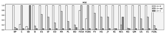
Figure 7. MSE scaled between 0 and 1.

Forecasting prices with LSTM. Strategies returns

From Table 4 below, we can see the comparison between returns with a different order of differencing using both strategies. This shows how much each data manipulation affected each symbol’s profitability. Strategies with d = 1 provide the best outcome.

Table 4. Strategy returns using LSTM predicted prices.

Symbol	Strategy No. 1			Strategy No. 2
	$\mathbf{d}=0$	$\mathbf{d}=\mathbf{opt}$	$\mathbf{d}=1$	$\mathbf{d}=0$	$\mathbf{d}=\mathbf{opt}$	$\mathbf{d}=1$
BP	−4.953	$-\mathbf{3.63}$	−4.420	$\mathbf{2.231}$	−4.218	−5.471
C	$\mathbf{4.715}$	−6.387	−10.452	−14.176	$\mathbf{0.980}$	−5.411
SB	−9.882	−10.886	$\mathbf{0.214}$	−26.0498	−3.776	$\mathbf{0.356}$
SI	$5.159$	$7.944$	$\mathbf{18.119}$	$2.932$	$10.044$	$\mathbf{21.583}$
ES	$-11.401$	$-7.629$	$-\mathbf{2.393}$	$-\mathbf{0.100}$	−12.803	−3.516
SF	$-3.374$	$\mathbf{1.960}$	$1.733$	$-4.015$	$\mathbf{2.360}$	$1.277$
ED	$0.006$	$-0.232$	$\mathbf{0.129}$	$0.087$	$0.181$	$\mathbf{0.269}$
RR	$2.221$	$1.118$	$\mathbf{5.719}$	$-1.663$	$\mathbf{4.774}$	3.331
PL	9.428	1.228	23.783	2.654	19.314	25.646
BO	$\mathbf{0.071}$	$-1.412$	$-7.898$	$\mathbf{0.125}$	$-4.540$	$-1.245$
FESX	$-3.3679$	$-0.196$	$\mathbf{2.933}$	$\mathbf{6.032}$	$1.687$	$2.992$
FGBS	$-0.2806$	$-\mathbf{0.003}$	$-0.596$	$-0.125$	$\mathbf{0.055}$	−0.547
FV	$-2.5998$	$-\mathbf{1.128}$	−2.4	$-2.789$	$-\mathbf{0.627}$	−3.023
HG	$-9.5296$	$-8.075$	$-\mathbf{7.531}$	$-6.385$	$-7.027$	$-\mathbf{0.968}$
JY	$-1.697$	$-0.836$	$\mathbf{0.442}$	$-2.719$	$-1.666$	$\mathbf{0.901}$
KC	−13.3799	$-\mathbf{12.387}$	$-29.527$	$-\mathbf{2.212}$	−15.932	−26.836
NE1	$3.265$	$\mathbf{3.707}$	$1.344$	$0.436$	$\mathbf{3.048}$	$2.166$
NG	$-15.061$	$\mathbf{7.439}$	$6.971$	$\mathbf{33.875}$	$14.393$	−1.366
QM	$-34.882$	−28.416	$-\mathbf{10.163}$	$-25.886$	−31.093	$-\mathbf{8.628}$
US	$\mathbf{3.223}$	$1.497$	$0.129$	$0.095$	$\mathbf{3.866}$	−1.414
EC	$-0.835$	$3.036$	$\mathbf{3.150}$	$-5.925$	$2.523$	$\mathbf{3.367}$
FGBL	$-0.0538$	$0.954$	$\mathbf{1.070}$	$\mathbf{2.277}$	$1.823$	$1.691$
Win Count:	3	7	12	7	7	8

Forecasting prices with LSTM. Accuracy and MSE

Table 5 illustrates the results. Note that a huge variance between MSE was caused by a different tick size of future contracts and price range (Figure 8).

Table 5. Accuracy and MSE results of predicted prices.

Symbol	Accuracy			MSE
	d = 0	d = opt	d = 1	d = 0	d = opt	d = 1
BP	40.85	45.07	45.49	0.001	0.000	0.000
C	49.09	50.91	43.64	1.771	8.490	0.262
SB	49.63	54.81	54.81	0.041	0.040	0.051
SI	54.79	51.51	52.74	0.259	0.081	0.058
ES	32.88	37.95	36.07	1.791	1.407	0.794
SF	51.80	54.82	55.25	0.000	0.000	0.000
ED	46.46	49.28	49.71	0.021	0.006	0.001
RR	45.61	59.30	59.02	0.035	0.030	0.015
PL	42.47	53.01	61.04	8.307	3.449	1.241
BO	51.47	49.04	50.51	0.454	0.111	0.127
FESX	50.00	52.50	55.82	1.845	2.122	0.859
FGBS	45.24	44.52	42.92	0.004	0.008	0.001
FV	42.11	42.98	40.80	0.058	0.055	0.049
HG	46.60	47.18	47.57	0.001	0.001	0.001
JY	46.58	45.48	51.23	0.000	0.000	0.000
KC	48.00	46.40	43.01	4.469	0.410	0.406
NE1	49.04	58.85	57.23	0.000	0.000	0.000
NG	56.16	51.51	50.00	0.074	0.006	0.005
QM	49.32	50.41	56.77	1.971	1.670	1.377
US	53.42	53.01	50.62	3.762	2.037	0.763
EC	46.43	54.36	54.39	0.000	0.000	0.000
FGBL	53.62	54.57	52.17	0.816	0.313	0.237
Win Count:	6	6	10	0	3	19

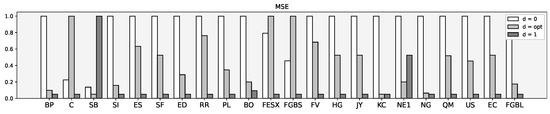
Figure 8. MSE scaled between 0 and 1.

Forecasting prices with XGBoost regressor: Strategy returns

XGBoost, also called Extreme Gradient Boosting, is a machine learning model that originated from Friedman et al. (2000) idea of gradient boosting used for regression and classification problems. We examined the XGBoost classifier for our datasets with window = 20. Each attempt was optimized accordingly on the validation sample. Results are depicted in Table 6.

Table 6. Strategy returns using LSTM predicted prices.

Symbol	Strategy No.1			Strategy No.2
	d = 0	d = opt	d = 1	d = 0	d = opt	d = 1
BP	$-5.469$	$-9.488$	$-\mathbf{4.249}$	$-5.286$	$-\mathbf{0.037}$	$-7.160$
C	$-7.535$	$\mathbf{8.118}$	$-8.518$	$-7.397$	$0.399$	$\mathbf{4.917}$
SB	$-9.350$	−12.053	$-\mathbf{6.298}$	−23.960	−13.049	$-\mathbf{1.238}$
SI	$3.486$	$\mathbf{35.727}$	$0.964$	$\mathbf{4.225}$	$1.424$	$2.566$
ES	$\mathbf{18.170}$	$-4.344$	−20.824	$\mathbf{1.599}$	$-9.179$	$-18.005$
SF	$0.780$	$4.153$	$\mathbf{4.825}$	$-0.411$	$1.001$	$\mathbf{1.823}$
ED	$0.075$	$\mathbf{0.304}$	$-0.320$	$0.124$	$\mathbf{0.180}$	$-0.050$
RR	$0.848$	$\mathbf{6.093}$	$2.142$	$-8.471$	$-1.610$	$\mathbf{0.878}$
PL	$-0.083$	$\mathbf{22.805}$	$12.050$	$17.619$	$\mathbf{20.204}$	$6.976$
BO	$-1.696$	$\mathbf{17.984}$	$-0.018$	$-9.518$	−17.838	$-\mathbf{6.782}$
FESX	$-6.728$	$-2.278$	$\mathbf{1.179}$	$-6.145$	$\mathbf{3.385}$	$-0.031$
FGBS	0.133	$-0.272$	$-0.476$	−0.155	$-0.281$	$-0.939$
FV	$-0.848$	$\mathbf{2.758}$	$-4.825$	$0.452$	$\mathbf{3.138}$	$-4.165$
HG	−26.104	$-9.468$	−8.455	$-\mathbf{5.488}$	−20.174	$-12.823$
JY	$-9.225$	$\mathbf{1.297}$	$0.625$	$-7.154$	$-4.731$	$\mathbf{1.106}$
KC	$-\mathbf{0.189}$	$-1.553$	−27.257	−32.046	−14.720	$-22.572$
NE1	$\mathbf{5.852}$	$-0.196$	$2.164$	$6.324$	$\mathbf{6.632}$	$0.989$
NG	$-0.362$	$12.753$	$\mathbf{14.640}$	$-0.362$	$\mathbf{6.909}$	$5.650$
QM	−27.229	−19.926	$-\mathbf{2.763}$	−25.197	$-2.976$	$\mathbf{4.016}$
US	$4.804$	$\mathbf{7.022}$	$-4.351$	$-5.313$	$\mathbf{6.336}$	$-4.927$
EC	$-6.784$	$\mathbf{2.700}$	$-2.018$	$-1.403$	$\mathbf{3.922}$	$-1.720$
FGBL	$-3.429$	$-0.046$	$\mathbf{2.164}$	$-4.727$	$\mathbf{2.015}$	$0.780$
Win Count:	4	10	8	4	11	7

Forecasting prices with XGBoost regressor: Accuracy and MSE

Table 7 illustrates the results. Note that a huge variance between MSE was caused by a different tick size of future contracts and price range (Figure 9).

Table 7. Accuracy and MSE results of predicted prices.

Symbol	Accuracy			MSE
	d = 0	d = opt	d = 1	d = 0	d = opt	d = 1
BP	50.70	39.44	45.07	0.002	0.000	0.000
C	41.82	52.35	42.95	1.468	1.143	0.498
SB	48.15	50.37	54.07	0.390	0.031	0.026
SI	56.16	60.27	46.58	0.173	0.211	0.091
ES	51.27	44.94	43.04	17.164	1.419	0.896
SF	60.27	53.57	55.40	0.000	0.000	0.000
ED	48.20	52.52	48.92	0.007	0.002	0.002
RR	51.47	56.14	59.65	0.047	0.018	0.010
PL	53.42	55.71	57.53	5.505	2.460	1.731
BO	47.37	58.82	49.26	0.369	0.178	0.107
FESX	44.93	50.72	51.39	35.623	1.150	0.855
FGBS	52.17	48.21	45.83	0.093	0.004	0.001
FV	47.86	50.29	39.18	0.123	0.101	0.054
HG	46.20	44.66	44.66	0.003	0.001	0.001
JY	41.43	50.68	47.95	0.000	0.000	0.000
KC	53.57	45.00	44.00	6.236	5.731	3.290
NE1	56.84	56.84	57.69	0.001	0.000	0.000
NG	56.73	54.05	50.68	0.123	0.004	0.003
QM	46.77	50.35	51.43	2.446	2.768	1.780
US	49.71	53.57	49.32	4.095	2.784	1.076
EC	41.52	53.80	49.32	0.001	0.000	0.000
FGBL	41.29	50.90	54.41	12.868	2.122	0.246
Win Count:	7	8	7	1	3	18

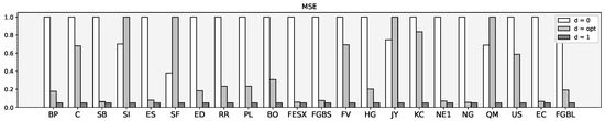
Figure 9. MSE scaled between 0 and 1.

Evaluating portfolio volatility

We can further analyze the risk of each strategy in regard to its prediction method. As Table 8 shows, both strategies show similar results in terms of volatility. As expected, the most consistent method with the difference time series is the first-order logarithmic (d = 1), providing the least amount of variance between the returns.

Table 8. Volatility.

	d = 0	d = opt	d = 1
LSTM strategy no.1	6.880	5.743	7.559
LSTM strategy no.2	8.465	7.548	7.239
XGB regressor strategy no.1	7.089	8.828	6.638
XGB regressor strategy no.2	7.917	6.745	5.451

Assuming returns are normally distributed, we can approximate the monthly value-at-risk with a 95% confidence level (Table 9).

Table 9. VaR 95%.

	d = 0	d = opt	d = 1
LSTM strategy no.1	6.880	5.743	7.559
LSTM strategy no.2	8.465	7.548	7.239
XGB regressor strategy no.1	7.089	8.828	6.638
XGB regressor strategy no.2	7.917	6.745	5.451

Neither data transformation shows a significantly lower risk. However, returns using time series transformation with $d=1$ with both LSTM and XGBoost predictors are the most stable. On average, all methods indicate about at least 5–8% loss every 20 months.

5. Conclusions

According to our research, machine learning algorithms should consider stationary time series transformations as it improved their predicted values. To deal with unknown values, algorithms must have a pool of known variables to find the best fitting estimation. In most cases, first-order difference of logarithmic data transformation $(d=1)$ showed the best results for each metric as the vast majority of symbols (more than 80%) had the best MSE value. One exception was XGBoost regressor, which was most profitable using fractional differencing as 45.45% of and 50% of all symbols earned more using two different strategies compared with other time series modifications.

Both transformations improved forecasting results in comparison with unmodified series. However, concluded results contradicted Marco López de Prado’s suggestion that saving memory in time series can lead to more accurate and profitable results compared to other methods.

For future works, we suggest further analyzing this topic since both transformations $(d=opt$ and $d=1)$ improved neural network predictions compared to raw data series $(d=0)$. One of the possibilities is the absence of long memory in future contract prices. Determining memory impact on the order of transformation and using supplementary tests would be beneficial for future research.

References

- Baillie, Richard T. 1996. Long memory processes and fractional integration in econometrics. Journal of Econometrics 73: 5–59. [Google Scholar] [CrossRef]
- Carreño Jara, Emiliano. 2011. Long memory time series forecasting by using genetic programming. Genetic Programming and Evolvable Machines 12: 429–56. [Google Scholar] [CrossRef]
- de Prado, Marcos Lopez. 2018. Advances in Financial Machine Learning. Hoboken: John Wiley & Sons. [Google Scholar]
- Friedman, Jerome, Hastie Trevor, and Robert Tibshirani. 2000. Additive logistic regression: A statistical view of boosting (with discussion and a rejoinder by the authors). The Annals of Statistics 28: 337–407. [Google Scholar] [CrossRef]
- Hosking, J. R. M. 1981. Fractional differencing. Biometrika 68: 165–76. [Google Scholar] [CrossRef]
- Kom Samo, Yves-Laurent. 2018. Stationarity and Memory in Financial Markets. October 15. Available online: https://towardsdatascience.com/non-stationarity-and-memory-in-financial-markets-fcef1fe76053 (accessed on 1 November 2022).
- Maynard, Alex, Aaron Smallwood, and Mark E. Wohar. 2013. Long memory regressors and predictive testing: A two-stage rebalancing approach. Econometric Reviews 32: 318–60. [Google Scholar] [CrossRef]
- Milionis, Alexandros E. 2004. The importance of variance stationarity in economic time series modelling. A practical approach. Applied Financial Economics 14: 265–78. [Google Scholar] [CrossRef]
- Sadaei, HosseinJavedani, Rasul Enayatifar, Frederico Gadelha Guimarães, Maqsood Mahmud, and Zakarya A. Alzamil. 2016. Combining ARFIMA models and fuzzy time series for the forecast of long memory time series. Neurocomputing 175: 782–96. [Google Scholar] [CrossRef]
- Salles, Rebecca, Kele Belloze, Fabio Porto, Pedro H. Gonzalez, and Eduardo Ogasawara. 2019. Nonstationary time series transformation methods: An experimental review. Knowledge-Based Systems 164: 274–91. [Google Scholar] [CrossRef]
Publisher’s Note: MDPI stays neutral with regard to jurisdictional claims in published maps and institutional affiliations. |
© 2022 by the authors. Licensee MDPI, Basel, Switzerland. This article is an open access article distributed under the terms and conditions of the Creative Commons Attribution (CC BY) license (https://creativecommons.org/licenses/by/4.0/).