Identification of Orbital Angular Momentum by Support Vector Machine in Ocean Turbulence

Abstract

With the advancement of underwater communication technology, the traditional modulation dimension has been introduced, developed and utilized. In addition, orbital angular momentum (OAM) is utilized as the modulation dimension for optical underwater communication to obtain larger spectrum resources. The OAM features are extracted using a histogram of oriented gradient and trained using the support vector machine method with a gradient direction histogram feature. The topological charge value of the OAM was used to identify the classification labels, and the ocean turbulence caused by different temperatures and salinity were analyzed. Experimentation results showed that the recognition accuracy for the OAM under the Laguerre–Gaussian beam rates of 1~5, 1~6, 1~7, 1~8, 1~9, and 1~10 was 98.93%, 98.89%, 97.33%, 96.66%, 95.40%, and 95.33%, respectively. The proposed method achieved a high recognition accuracy and performed efficiently under strong turbulence. Our research explored a new technique that provides a new idea for the demodulation of OAM in optical underwater communication.

1. Introduction

In traditional wireless optical communication, basic information modulation dimensional resources of light waves (amplitude, frequency, wavelength, polarization, and time, etc.) have been developed and utilized. The new spatial information modulation based on orbital angular momentum (OAM) has received extensive attention from the academic community [1,2,3]. The most representative OAM beam is the Laguerre–Gaussian (LG) beam, in which the LG beam is selected as the research object under the underwater channel. The OAM mode value of each photon can be any integer, and different OAM modes are orthogonal to each other. This implies that different OAM modes will not interfere with each other during transmission [4,5,6], so OAM light can be applied to the coding, decoding, and multiplexing transmission of wireless optical communication [7,8,9,10] to meet the ever-increasing demand of information transmission capacity. Unfortunately, OAM suffers from rich information that is mainly caused by the anti-interference ability of the OAM beam and transmission interference. In a challenging situation such as in a complex and changing underwater environment, the beams interfere with the OAM during the transmission process [11,12,13,14,15], thereby increasing the difficulty of the receiver to identify the OAM, and thus, making the identification of the OAM an important process.

The well-established technique of identifying OAM is generally to detect the number of bright fringes that appear in the intensity pattern after the vortex beam passes through the grating. Due to the influence of turbulence, the transceiver is required to be highly aligned, which often results in low identification of the OAM. Integrating neural network technology to identify OAM has proven to be promising with high accuracy [16,17,18,19,20]. The authors in [21,22,23] introduced an OAM recognition method based on a feedforward neural network (FNN). Both CNN and FNN have high accuracy, but there are limitations due to the quest for large training samples and high complexity. On the other hand, the machine learning technique has a good robustness with small datasets and it is capable of extracting the feature vector of trained samples [24,25,26]. Investigation shows that spatial distribution of OAM beams under ocean turbulence can be identified by analyzing the phase space distribution of the beams under turbulence.

Based on the support vector machine (SVM) model, this paper implements a method to identify the OAM mode using the histogram of oriented gradient (HOG) [27,28,29,30]. The results show that obtaining the HOG feature of the spatial phase map is valuable in the OAM modal identification.

2. Basic Theory

2.1. LG Beam

In cylindrical coordinates, the LG beam propagating along the z-axis can be expressed as:

$$\begin{array}{l}L{G}_p^L(r,\theta ,z)=\frac{C}{\sqrt{1+z^2/z_R{}^2}}{\left[\frac{r\sqrt{2}}{w(z)}\right]}^{\left|L\right|}{L}_p^L\left[\frac{2r^2}{w^2(z)}\right]\exp \left[\frac{-r^2}{w^2(z)}\right]\times \exp \left[\frac{ik{r}^{2}z}{2(z^2+z_R^2)}\right]\\ \times \exp (iL\theta )\exp \left[-i(2p+L+1)\arctan \frac{z}{z_R}\right]\end{array}$$

(1)

$w(z)=\sqrt{2(z^2+z_R^2)/k{z}_R}$ is the beam waist radius after the distance of z is transmitted; $z_R=k{w}_0^2/2$ is the Rayleigh length; $w_0$ is the zero-order beam waist radius, which is the beam radius when the transmission distance z = 0; $k=2\pi /\lambda$ is the beam, L is the topology of the beam; $p$ is the radial factor, which represents the phase change in the beam along the radial direction; $\mathrm{C}=\sqrt{2p!/[\pi (\left|L\right|+p)!]}$ is the normalization factor; ${\left[r\sqrt{2}/w\left(z\right)\right]}^{\left|L\right|}$ is affected by the phase singularity vortex kernel function; $L_p^L$ denotes the Laguerre polynomial; $\exp \left(iL\theta \right)$ helical phase factor, i is the imaginary unit; and $\theta$ is the directional phase angle, which indicates that the beam carries an OAM.

2.2. Basic Principles of SVM

SVM is a machine model for classifying data based on statistical theory. The basic idea of SVM is to find the point that can make all points closest to the hyperplane with the largest interval.

As can be seen from Figure 1, the red triangular data points represent the “$y=+1$” class, and the blue circular data points represent the “$y=-1$” class. The SVM classification hyperplane for these two types of data can be expressed by Equation (2).

$$f(x)=w^{T}x+b$$

(2)

where $w$ is the normal vector of the classification hyperplane, and $b$ is the intercept. When $f\left(x\right)$ is greater than or equal to 0, data point $x$ belongs to class “$y=+1$”; for data points $x$ where $f\left(x\right)$ is less than 0, it belongs to class “$y=-1$”. Therefore, the maximum spacing hyperplane can be obtained by solving the variables $w$ and $b$, to realize the classification of data points in the plane.

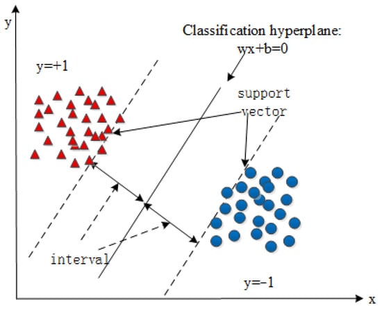
Figure 1. Schematic diagram of SVM classification.

To facilitate the calculation, ${\Vert w\Vert }^2$is used for subsequent solutions. The objective function to obtain the maximum interval classification is:

$$\min \frac{1}{2}{\Vert w\Vert }^2$$

(3)

$$s.t.\hspace{1em}{y}_i\left(w^T{x}_i+b\right)\ge 1,i=1,2,\dots ,N$$

(4)

$x_i$ is the $i$-th eigenvector of the data, and $y_i$ is the category to which the $i$-th data point belongs (+1 or −1). The objective function is a convex quadratic programming problem. The Lagrange multiplier method is used to convert, and transform the problem into a dual problem to be solved. The optimal solution of the objective function is obtained by solving its dual problem.

For the above transformed objective function, its Lagrange function can be expressed as:

$$L(w,b,\alpha )=\frac{1}{2}{\Vert w\Vert }^2-{\displaystyle \sum _{i=1}^N{\alpha }_i}{y}_i(w^T{x}_i+b)+{\displaystyle \sum _{i=1}^N{\alpha }_i},\hspace{1em}i=1,2,\dots ,N$$

(5)

$\alpha ={({\alpha }_1,{\alpha }_2,\dots ,{\alpha }_N)}^T$ is the Lagrange multiplier vector, $L(w,b,\alpha )$is the Lagrange function. Partial derivatives is taken so as to obtain the parameters w and $b$, and finally the classification function is obtained as:

$$\begin{array}{ll}f(x)& ={({\displaystyle \sum _{i=1}^N{\alpha }_i{y}_i}{x}_i)}^{T}x+b\\ & ={\displaystyle \sum _{i=1}^N{\alpha }_i{y}_i}<x_i,x>+b\end{array}$$

(6)

2.3. HOG Features

HOG features are constructed by calculating and counting the local regional gradient of the image. The main purpose of the HOG algorithm is to calculate the gradient of the image to obtain the gradient information of the image as a feature [21]. The gradient of the pixel in the image is:

$$G_x(x,y)=H(x+1,y)-H(x-1,y)$$

(7)

$$G_y(x,y)=H(x,y+1)-H(x,y-1)$$

(8)

where $G_x(x,y)$, $G_y(x,y)$, and $H(x,y)$ represent the horizontal gradient, vertical gradient and pixel value at pixel $(x,y)$ in the input image, respectively. The gradient magnitude and gradient direction at pixel $(x,y)$ are:

$$G(x,y)=\sqrt{G_x{(x,y)}^2+G_y{(x,y)}^2}$$

(9)

$$\alpha (x,y)={\tan }^{-1}(\frac{G_y(x,y)}{G_y(x,y)})$$

(10)

As shown in Figure 2, the image is divided into small cells, and the gradient histogram of the cell is calculated to form the HOG feature of the cell. The gradient direction of the cell is divided into the gradient of the interval, and a cell can be obtained.

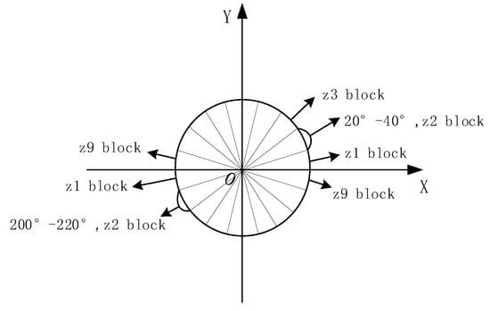
Figure 2. Gradient direction division interval.

As shown in Figure 3, every few cells are formed into a block (for example, 3 × 3 cells/block), and the feature vectors of all cells in a block are concatenated to obtain the HOG feature vector of the block.

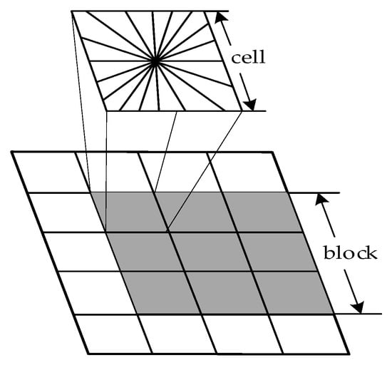
Figure 3. Cell unit building blocks.

Figure 4 shows the HOG feature extraction under ocean turbulence.

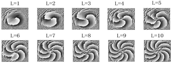
Figure 4. Spatial phase map HOG characteristics of different OAM modes (L = 1~10) under ocean turbulence.

3. LG Beam Pattern Recognition Simulation Design

3.1. Ocean Turbulence Random Phase Screen Model

In free-space transmission without turbulence, the normalized function of the beam on the transmission axis is almost the same as that at the light source. The phase and intensity of the beam are not affected. The intensity perturbation of the beam is small, but the phase perturbation is large. Furthermore, the influence of the ocean turbulence on the beam transmission can be approximated as a pure phase perturbation [11], so that the beam can pass through a series of equidistant random phase screens. To simulate the influence of ocean turbulence on beam transmission, as shown in Figure 5, the ocean turbulence model was constructed by the power spectrum inversion method, and the experimental simulation of the OAM identification under the ocean turbulence channel was carried out based on MATLAB.

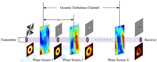
Figure 5. Ocean turbulence random phase screen model.

It is assumed that the plane where the phase screen is located is the $XY$ plane, and the beam propagates in the z-axis direction. In the spatial domain, the light field of the initial beam is $U_0(x,y)$. $U_0(x,y)$ is a complex number, and the magnitude of the modulus value represents the intensity of the light field. The angle represents the spatial phase of the light field. Assuming that the light beam propagates in the free-space channel, and the transfer function in the spatial frequency domain is $U_{prop}(k_x,k_y)$. The light beam only propagates in free space before reaching the first phase screen. The light field when it reaches the first phase screen can be expressed as:

$$U_{1-}(x,y)=F^{-1}\{F[U_0(x,y)]\times U_{prop}(k_x,k_y)\}$$

(11)

$k_x$ and $k_y$ are the frequency components of the $X$-axis and $Y$-axis directions in the spatial frequency domain, respectively. $F$ represents the Fourier transform, and $F^{-1}$ represents the inverse Fourier transform. $U_{prop}(k_x,k_y)$ is the free-space transfer function, which is expressed as:

$$U_{prop}=\exp (i\Delta z\sqrt{k^2-k_x{}^2-k_y{}^2})$$

(12)

After the light beam passes through the phase screen, the spatial phase of its light field is affected by the phase screen model, and the change in the light field is expressed as:

$$U_{1+}(x,y)=U_{1-}(x,y)\times i\phi (x,y)$$

(13)

where $\phi (x,y)$ is the distribution function of the random phase screen.

Based on the power spectrum inversion method, to generate a phase screen, a Hermitian complex Gaussian random number matrix $H\left(k_x,k_y\right)$ with zero mean and a unit variance of 1 is generated in the frequency domain. In addition, $H\left(k_x,k_y\right)$ is filtered by the seawater phase spectrum function $F_{\Phi }\left(k_x,k_y\right)$ that conforms to the Kolmogorov spectrum of ocean turbulence. Then, the inverse Fourier transform is perform to obtain the ocean turbulence random phase screen $\varphi \left(x,y\right)$, which can be expressed as:

$$\varphi \left(x,y\right)=C{\displaystyle {\sum }_{k_x}{\displaystyle {\sum }_{k_y}H\left(k,k_y\right)}}\sqrt{F_{\Phi }\left(k_x,k_y\right)}\exp \left[j\left(k_{x}x+k_{y}y\right)\right]$$

(14)

We generate a Gaussian random number matrix with $N\times N$ of mean value 0, variance 1 by randn ( ), and then perform Fourier transform (FFT) to obtain $H\left(k_x,k_y\right)$.

The seawater phase spectrum $F_{\Phi }\left(k_x,k_y\right)$ on the slice plane perpendicular to the propagation direction of the beam can be expressed as:

$$F_{\Phi }\left(k_x,k_y\right)=2\pi k^2\Delta z\Phi (k_x,k_y)$$

(15)

$k=2\pi /\lambda$ is the light beam, $k_x$ and $k_y$ represent the beam in the direction of $x,y$; $\Delta z$ is the propagation distance of the beam; $\Phi \left(k_x,k_y\right)$ is the refractive index fluctuation spectrum of seawater.

The common seawater refractive index fluctuation spectrum was proposed by [13], and its expression is:

$$\begin{gathered} \Phi (k_x,k_y)=0.388\times {10}^{-8}{\epsilon }^{-1/3}{(\sqrt{k_x^2+k_y^2})}^{-11/3}[1+2.35(\sqrt{k_x^2+k_y^2}\eta )2/3]\times \\ \frac{{\chi }_T}{w^2}(w^2{e}^{-AT\delta }+e^{-AS\delta }-2w{e}^{-ATS\delta }) \end{gathered}$$

(16)

Among them, $\epsilon$ is the kinetic energy dissipation rate per unit volume of seawater with a range of $\epsilon$$[{10}^{-10}{\mathrm{m}}^2/{\mathrm{s}}^3,{10}^{-1}{\mathrm{m}}^2/{\mathrm{s}}^3]$; ${\chi }_T$ is the mean square seawater temperature dissipation rate, with a range of ${\chi }_T$$[{10}^{-10}{\mathrm{K}}^2/\mathrm{s},{10}^{-4}{\mathrm{K}}^2/\mathrm{s}]$; $w$ is the turbulence caused by the change in temperature gradient and salinity gradient, with a range of $w$$\left[-5, 0\right]$; $\eta$ is the Kolmogorov microscale, with a range of $\left[6\times {10}^{-3}\mathrm{m}, 0.01\mathrm{m}\right]$; the value range of the Kolmogorov scale is $\eta$; and the Kolmogorov scale in the deep seawater is close to 0.01 m. Other parameters are set to: $A_S=1.9\times {10}^{-4}$

$$A_T=1.863\times {10}^{-2},A_{TS}=9.41\times {10}^{-3},\delta =8.284\times {(\sqrt{k_x^2+k_y^2}\eta )}^{3/4}+12.978{(\sqrt{k_x^2+k_y^2}\eta )}^2)$$

$C_n^2$ is the equivalent temperature structure parameter, also known as the turbulence intensity, and its expression is:

$$C_n^2={10}^{-8}{\chi }_T{\epsilon }^{-1/3}$$

(17)

3.2. Simulation Analysis

The spatial phase map of OAM mode is obtained by constructing a random phase screen model of ocean turbulence, and HOG feature extraction is performed on the phase map. The data volume used for the experimentation is as follows: (1) 250 pieces of 1~5 OAM modalities; (2) 300 pieces of 1~6 OAM modalities; (3) 350 pieces of 1~7 OAM modalities; (4) 400 pieces of 1~8 OAM modalities; (5) 450 pieces of 1~9 OAM modalities; and (6) 500 pieces of 1~10 OAM modalities.. In order to make the data accurate and reliable, five simulations were carried out and the average result was taken. The obtained data sample set was divided into a training set and test set according to the ratio of 7:3. Based on the influence of different $w$ on the OAM modal recognition rate, we trained the model under the transmission distance, and the OAM mode recognition rate is obtained when the turbulence intensity is equals to the strong turbulence $C_n^2=1.0\times {10}^{-13}{\mathrm{K}}^2{\mathrm{m}}^{-2/3}$.

According to Figure 6a,b, when the ocean turbulence intensity is $C_n^2=1.0\times {10}^{-13}$ ${\mathrm{K}}^2{\mathrm{m}}^{-2/3}$, the OAM single mode recognition rate under different w values is $w$ = −2.0. It can clearly be seen that the OAM mode is less affected by $w$, and the OAM modality recognition rates of L = 1, 2, 3, 4, and 5 have higher recognition rates of 100%, 100%, 100%, 100%, 100%, and 94.64%. In addition, L = 1, 2, 3, 4, 5, and 6 recognition rates achieves 100%, 100%, 100%, 100%, 98.66%, and 94.66%, respectively. When $w$ = −1.75, it has little effect on the OAM modal recognition rate. On the whole, the OAM modal recognition rate gradually decreases with the increase in $w$.

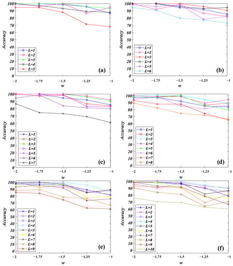
Figure 6. OAM single mode recognition rate under different values: (a) L = 1~5; (b) L = 1~6; (c) L = 1~7; (d) L = 1~8; (e) L = 1~9; (f) L = 1~10.

According to Figure 6c,d, when the ocean turbulence intensity is $C_n^2=1.0\times {10}^{-13}$ ${\mathrm{K}}^2{\mathrm{m}}^{-2/3}$, we obtained varying values for the OAM single mode recognition rate under varying $w$ and L values, especially when L = 1, 2, 3, 4, 5, 6, and 7. When the modal was $w$ = −2.0, the OAM modal was less affected by $w$, and the OAM modal recognition rate had a higher recognition rate of 100%, 100%, 100%, 100%, 100%, 94.66%, and 86.66%. When $w$ = −2.0, the OAM mode was less affected by $w$, and the OAM mode recognition rate was higher. The recognition rates obtained were 97.34%, 100%, 100%, 100%, 98.66%, 94.66%, 93.32%, and 89.32%. In Figure 6c, the OAM modal recognition rate declined relatively gently, and in Figure 6d L = 1 and 3, the OAM modal recognition rate decreased relatively gently, and later fluctuated greatly, but basically the OAM modal recognition rate gradually decreased with the increase in $w$.

According to Figure 6e,f, when the ocean turbulence intensity is $C_n^2=1.0\times {10}^{-13}$ ${\mathrm{K}}^2{\mathrm{m}}^{-2/3}$, we obtained varying values for the OAM single mode recognition rate under varying w and L values, especially when L = 1, 2, 3, 4, 5, 6, 7, 8,and 9. The OAM mode in the case of $w$ = −2.0, $w$ = −1.75, it can be clearly seen that the OAM mode was less affected by $w$, and the OAM mode recognition rate remained relatively stable. When $w$ = −1.5 and −1.25, it had a greater impact on the OAM modal recognition rate, and the decline was larger; when the OAM modalities of L = 1, 2, 3, 4, 5, 6, 7, 8, 9, and 10 are at $w$ = −2.0, $w$ = −1.75, and $w$ = −1.5, it can be clearly seen that the OAM mode was less affected by w, and the rate of decline was relatively gentle. To sum up, looking at Figure 6a–f, the larger the L value of OAM mode, the lower the recognition accuracy, and most of the OAM modal recognition rates gradually decreased with the increase in $w$, and there are a small part of the OAM modal recognition rates that fluctuated up and down, which was caused by the random generation of ocean turbulence.

As shown in Table 1, the OAM multimodal recognition rate under the ocean turbulence channel is characterized. Combined with Figure 6, according to the data shown in Table 1, the experimental results show that in the ocean turbulence channel, with the increase in the value of $w$, the spatial phase distribution of the OAM mode is seriously damaged. The rate decreases accordingly, and the larger the topological charge value, the lower the recognition rate of the OAM mode.

Table 1. Recognition accuracy of OAM multimodality.

$\mathit{w}$	L = 1~5	L = 1~6	L = 1~7	L = 1~8	L = 1~9	L = 1~10
−2.0	0.9893	0.9889	0.9733	0.9666	0.9540	0.9533
−1.75	0.9759	0.9644	0.9581	0.9516	0.9466	0.9240
−1.5	0.9600	0.9466	0.9276	0.9217	0.9214	0.9133
−1.25	0.8792	0.8726	0.8656	0.8383	0.8148	0.8017
−1.0	0.8613	0.8488	0.8228	0.8199	0.7896	0.7854

As shown in Figure 7, the OAM (L = 1~5, 1~6, 1~7, 1~8, 1~9, 1~10) multi-modal recognition rate change trend under different $w$ values can be seen. With the increase in $w$, the OAM modal recognition accuracy gradually decreased, and with the increase in OAM modality, the recognition accuracy also gradually decreased. When the OAM modality was 1~10, the recognition rate decreased from 95.33% to 78.54%.

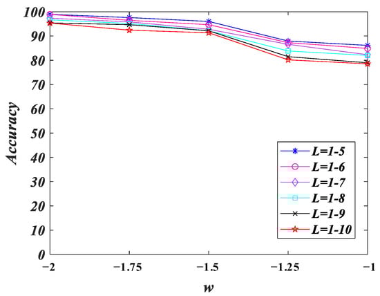
Figure 7. OAM (L = 1~5, 1~6, 1~7, 1~8, 1~9, 1~10) modal recognition rate under different $w$ values.

By simulating the transmission of LG beams under ocean turbulence, the OAM mode recognition rate of SVM was analyzed. In the case of turbulence is $C_n^2=1.0\times {10}^{-13}{\mathrm{K}}^2{\mathrm{m}}^{-2/3}$, the degree of damage to the spatial phase diagram of the OAM mode was different under different $w$.When $w$ = −2.0, the ocean turbulence intensity had little effect on the spatial distribution characteristics of the OAM beams. The classification and recognition rate of SVM with L = 1~5 can reach 98.93%, L = 1~6 can reach 98.89%, L = 1~7 can reach 97.33%, L = 1 to 8 can reach 96.66%, L = 1 to 9 can reach 95.4%, and L = 1 to 10 can reach 95.33%. If it increases, the spatial phase distribution of the OAM mode is seriously damaged, resulting in different degrees of dispersion, and a gradual decline in the SVM recognition accuracy.

4. Conclusions

In this paper, the OAM modal recognition of ocean turbulence based on SVM, and the OAM modal recognition simulation under the ocean turbulence channel was carried out. The influence of strong turbulence on the OAM modal recognition was analyzed. The results show that the accuracy of the OAM modal recognition gradually increased with the decrease in $w$. With the increase in the OAM modes, the recognition accuracy also gradually decreased. According to the experimental results, new ideas can be provided for the demodulation and research of optical underwater communication, which has high experimental and research application value.

References

- Wang, A.; Zhu, L.; Zhao, Y.; Li, S.; Lv, W.; Xu, J.; Wang, J. Adaptive water-air-water data information transfer using orbital angular momentum. Opt. Express 2018, 26, 8669–8678. [Google Scholar] [CrossRef] [PubMed]
- Wang, W.; Wang, P.; Cao, T.; Tian, H.; Zhang, Y.; Guo, L. Performance Investigation of Underwater Wireless Optical Communication System Using M-ary OAMSK Modulation Over Oceanic Turbulence. IEEE Photonics J. 2017, 9, 1–15. [Google Scholar] [CrossRef]
- Li, M. On Performance of Optical Wireless Communication With Spatial Multiplexing Towards 5G. IEEE Access 2018, 6, 28108–28113. [Google Scholar] [CrossRef]
- Zhao, Y.; Xu, J.; Wang, A.; Lv, W.; Zhu, L.; Li, S.; Wang, J. Demonstration of data-carrying orbital angular momentum-based underwater wireless optical multicasting link. Opt. Express 2017, 25, 28743–28751. [Google Scholar] [CrossRef]
- Yao, A.M.; Miles, J.P. Orbital Angular Momentum-Origins, Behavior and Applications. Adv. Opt. Photonics 2011, 3, 161–204. [Google Scholar] [CrossRef]
- Cui, X.; Yin, X.; Chang, H.; Guo, Y.; Zheng, Z.; Sun, Z.; Liu, G.; Wang, Y. Analysis of an adaptive orbital angular momentum shift keying decoder based on machine learning under oceanic turbulence channels. Opt. Commun. 2018, 429, 138–143. [Google Scholar] [CrossRef]
- Yan, Y.; Yue, Y.; Huang, H. Alan Willner. Multicasting in a Spatial Division Multiplexing System based on Optical Orbital Angular Momentum. Opt. Lett. 2013, 19, 3930–3933. [Google Scholar] [CrossRef] [PubMed]
- Baghdady, J.; Miller, K.; Kelly, J.; Srimathi, I.R.; Li, W.; Johnson, E.G. Underwater Optical Communication Link Using Wavelength Division Multiplexing, Polarization Division Multiplexing and Orbital Angular Momentum Multiplexing. In Proceedings of the Frontiers in Optics 2016, OSA Technical Digest (online) (Optica Publishing Group, 2016), paper FTh4E.4. Rochester, NY, USA, 17–21 October 2016. [Google Scholar] [CrossRef]
- Ren, Y.; Li, L.; Zhao, Z.; Xie, G.; Wang, Z.; Ahmed, N.; Yan, Y.; Cao, Y.; Willner, A.J.; Liu, C.; et al. 4 Gbit/s Underwater Optical Transmission Using OAM Multiplexing and Directly Modulated Green Laser. In Proceedings of the Conference on Lasers and Electro-Optics, OSA Technical Digest (2016) (Optica Publishing Group, 2016), paper SW1F.4. San Jose, CA, USA, 5–10 June 2016. [Google Scholar] [CrossRef]
- Wang, W.; Wang, P.; Guo, L. Performance Investigation of OAMSK Modulated Wireless Optical System over Turbulent Ocean Using Convolutional Neural Networks. J. Lightwave Technol. 2020, 38, 1753–1765. [Google Scholar] [CrossRef]
- Sun, R.; Guo, L.; Cheng, M.; Li, J. Multiple Random Phase-Screen Simulation of Scintillation Effect of Bessel-Gaussian Beam in Ocean Turbulence. In Proceedings of the 2018 12th International Symposium on Antennas, Propagation and EM Theory (ISAPE), Hangzhou, China, 3–6 December 2018; pp. 1–4. [Google Scholar] [CrossRef]
- Cheng, M.; Guo, L.; Li, J.; Zhang, Y. Channel Capacity of the OAM-Based Free-Space Optical Communication Links With Bessel–Gauss Beams in Turbulent Ocean. IEEE Photonics J. 2016, 8, 1–11. [Google Scholar] [CrossRef]
- Nikishov, V.V.; Nikishov, V.I. Spectrum of turbulent fluctuations of the seawater refraction index. Int. J. Fluid Mech. Res. 2000, 27, 82–98. [Google Scholar] [CrossRef]
- Baykal, Y. Higher order mode laser beam intensity fluctuations in strong oceanic turbulence. Opt. Commun. 2017, 390, 72–75. [Google Scholar] [CrossRef]
- Li, Y.; Yu, L.; Zhang, Y. Influence of anisotropic turbulence on the orbital angular momentum modes of Hermite-Gaussian vortex beam in the ocean. Optics express 2017, 11, 12203–12215. [Google Scholar] [CrossRef] [PubMed]
- Xiong, W. Convolutional Neural Network Assisted Optical Orbital Angular Momentum Identification of Vortex Beams. IEEE Access 2020, 8, 193801–193812. [Google Scholar] [CrossRef]
- Wang, P. Convolutional Neural Network-Assisted Optical Orbital Angular Momentum Recognition and Communication. IEEE Access 2019, 7, 162025–162035. [Google Scholar] [CrossRef]
- Wang, Z.; Guo, Z. Adaptive Demodulation Technique for Efficiently Detecting Orbital Angular Momentum (OAM) Modes Based on the Improved Convolutional Neural Network. IEEE Access 2019, 7, 163633–163643. [Google Scholar] [CrossRef]
- Wang, Z. Efficient Recognition of the Propagated Orbital Angular Momentum Modes in Turbulences With the Convolutional Neural Network. IEEE Photonics J. 2019, 11, 1–14. [Google Scholar] [CrossRef]
- Liu, W.; Jin, M.; Hao, Y.H. Efficient identification of orbital angular momentum modes carried by Bessel Gaussian beams in oceanic turbulence channels using convolutional neural network. Opt. Commun. 2021, 498, 127251. [Google Scholar] [CrossRef]
- He, Y.; Liu, J.; Wang, X.; Wu, Y.; Zhou, X.; Cheng, Y.; Gao, Y.; Li, Y.; Chen, S.; Fan, D. Detecting Orbital Angular Momentum Modes of Vortex Beams Using Feed-Forward Neural Network. J. Lightwave Technol. 2019, 37, 5848–5855. [Google Scholar] [CrossRef]
- Huang, Z.; Wang, P.; Liu, J.; Xiong, W.; He, Y.; Zhou, X.; Xiao, J.; Li, Y.; Chen, S.; Fan, D. Identification of hybrid orbital angular momentum modes with deep feedforward neural network. Results Phys. 2019, 15, 102790. [Google Scholar] [CrossRef]
- Jing, G.; Chen, L.; Wang, P.; Xiong, W.; Huang, Z.; Liu, J.; Chen, Y.; Li, Y.; Fan, D.; Chen, S. Recognizing fractional orbital angular momentum using feed forward neural network. Results Phys. 2021, 28, 104619. [Google Scholar] [CrossRef]
- Li, J.; Zhang, M.; Wang, D. Adaptive Demodulator Using Machine Learning for Orbital Angular Momentum Shift Keying. IEEE Photonics Technol. Lett. 2017, 17, 1455–1458. [Google Scholar] [CrossRef]
- Sun, R.; Guo, L.; Cheng, M.; Li, J.; Yan, X. Identifying orbital angular momentum modes in turbulence with high accuracy via machine learning. J. Opt. 2019, 21, 075703. [Google Scholar] [CrossRef]
- Wang, S.; Guo, X.; Tie, Y.; Lee, I.; Qi, L.; Guan, L. Graph-Based Safe Support Vector Machine for Multiple Classes. IEEE Access 2018, 6, 28097–28107. [Google Scholar] [CrossRef]
- Feng, K.; Yuan, F. Static hand gesture recognition based on HOG characters and support vector machines. In Proceedings of the 2013 2nd International Symposium on Instrumentation and Measurement, Sensor Network and Automation (IMSNA), Toronto, ON, Canada, 23–24 December 2013; pp. 936–938. [Google Scholar] [CrossRef]
- Li, B.; Huo, G. Face recognition using locality sensitive histograms of oriented gradients. Opt. -Int. J. Light Elect 2016, 6, 3489–3494. [Google Scholar] [CrossRef]
- Xiang, Z.; Tan, H.; Ye, W. The Excellent Properties of a Dense Grid-Based HOG Feature on Face Recognition Compared to Gabor and LBP. IEEE Access 2018, 6, 29306–29319. [Google Scholar] [CrossRef]
- Awais, M. Real-Time Surveillance Through Face Recognition Using HOG and Feedforward Neural Networks. IEEE Access 2019, 7, 121236–121244. [Google Scholar] [CrossRef]
Publisher’s Note: MDPI stays neutral with regard to jurisdictional claims in published maps and institutional affiliations. |
© 2022 by the authors. Licensee MDPI, Basel, Switzerland. This article is an open access article distributed under the terms and conditions of the Creative Commons Attribution (CC BY) license (https://creativecommons.org/licenses/by/4.0/).