Article

Accessing the Impact of Meteorological Variables on Machine Learning Flood Susceptibility Mapping

Natural Resources Canada, Ottawa, ON K1S 5K2, Canada
*
Author to whom correspondence should be addressed.
Remote Sens. 2022, 14(7), 1656; https://doi.org/10.3390/rs14071656
Submission received: 28 January 2022 / Revised: 22 March 2022 / Accepted: 28 March 2022 / Published: 30 March 2022
(This article belongs to the Special Issue Artificial Intelligence and Remote Sensing Datasets)

Abstract

:
Machine learning (ML) algorithms have emerged as competent tools for identifying areas that are susceptible to flooding. The primary variables considered in most of these works include terrain models, lithology, river networks and land use. While several recent studies include average annual rainfall and/or temperature, other meteorological information such as snow accumulation and short-term intense rain events that may influence the hydrology of the area under investigation have not been considered. Notably, in Canada, most inland flooding occurs during the freshet, due to the melting of an accumulated snowpack coupled with heavy rainfall. Therefore, in this study the impact of several climate variables along with various hydro-geomorphological (HG) variables were tested to determine the impact of their inclusion. Three tests were run: only HG variables, the addition of annual average temperature and precipitation (HG-PT), and the inclusion of six other meteorological datasets (HG-8M) on five study areas across Canada. In HG-PT, both precipitation and temperature were selected as important in every study area, while in HG-8M a minimum of three meteorological datasets were considered important in each study area. Notably, as the meteorological variables were added, many of the initial HG variables were dropped from the selection set. The accuracy, F1, true skill and Area Under the Curve (AUC) were marginally improved when the meteorological data was added to the a parallel random forest algorithm (parRF). When the model is applied to new data, the estimated accuracy of the prediction is higher in HG-8M, indicating that inclusion of relevant, local meteorological datasets improves the result.

1. Introduction

As the frequency and intensity of flooding is increasing around the globe, it has become increasingly important to have an understanding of the areas most prone or susceptible to flooding. Identification of flood prone areas and priority setting for flood mapping is one of the key steps outlined by the Canadian Federal Flood Mapping Guidelines being developed by Natural Resources Canada (NRCan) and Public Safety Canada (PSC) [1].
While hydraulic and hydrologic (H&H) models provide detailed assessments of specific areas at risk of flooding under certain circumstances, the spatial coverage provided by these models is generally limited to a watershed or sub-watershed and the outputs are based on user-defined scenarios. Data inputs required for these models to accurately describe the hydrology of the local environment may include measurements of precipitation, temperature, snow water equivalent, water levels, discharge and groundwater measurements [2].
Alternative methods have been proposed to cover various scales, e.g., macro (national) or meso (province, watershed) scale, and can generate a continuous surface, such that users can identify areas that are most prone to flooding in order to prioritize data collection and flood mapping [3].
Several macro and meso studies have used GIS weighting criteria [4,5,6] or multi-criteria decision making [7] to produce flood susceptibility maps. A potential disadvantage of using these traditional weighting methods is that expert opinion is required to assign weights and/or create classifications of the input datasets. Challenges to this method may arise with finding experts and/or with those of differing background and experience assigning differing weights/categories [8], resulting in differing maps.
The advance of computing technologies coupled with a growing archive of data have led to an environment suited to the iterative aspect of machine learning (ML) in order to exploit its capabilities to identify patterns in data and generate predictions. In addition, ML approaches remove the reliance on expert opinion for classification and weighting of the input data layers. Recently, many researchers have explored the use of ML to improve awareness of flooding, from flash flooding [9,10], stream flow simulations [11], flood risk assessments [12] and flood susceptibility [13,14,15,16].
While there is a growing body of literature of ML being applied to flood susceptibility mapping, there is great variability in many components of the process, including the data sets considered, the most suitable ML algorithm to use and selection of appropriate evaluation criteria. Most published studies concur on certain basic data layers necessary to describe flood susceptibility and that multiple models should be applied to a study area to determine the most appropriate model for a region. In most studies, these datasets include a digital terrain model (DTM), some measurement of the hydrographic network (distance to river, river density or stream power index), and some descriptor of the geology or lithology, Figure 1. In addition, several DTM derivatives may be considered: slope, aspect, curvature and terrain wetness index (TWI). Several recent publications have included mean annual rainfall and precipitation [14,15,17,18,19,20,21]. Only one paper, [13], was found to consider other meteorolgoical data such as daily precipitation and frequency of heavy rain.
Given that the development of flood hazard maps includes H&H modelling to account for water input and timing as water flows through the system to generate a flood map, one might ask why these data have not been explored in flood susceptibility mapping. Especially, considering in Canada, most flooding occurs in the spring as temperatures rise, snowpack melts and heavy precipitation falls.
Thus, the objective of this paper is to evaluate the impact of meteorological datasets on flood susceptibility prediction, as it is hypothesized that exclusion of these factors limits the quality of the prediction. The remainder of the paper is structured as follows: in Section 2, the datasets, machine learning model and evaluation metrics are described. In Section 3, the five study areas are introduced. In Section 4, the results are presented, and in Section 5, the results are discussed.

2. Materials and Methods

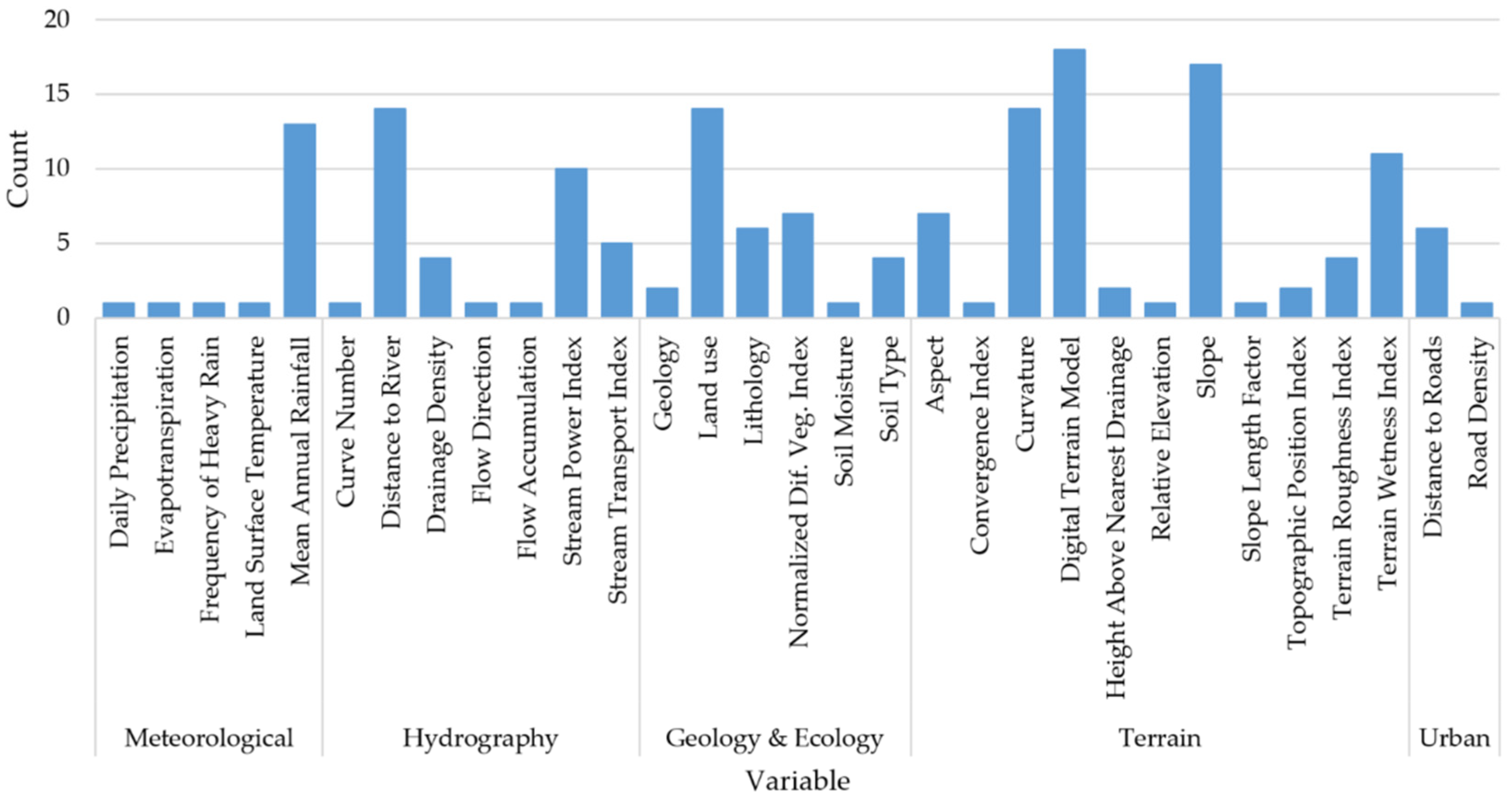
2.1. Exploratory Variables

A list of exploratory variables was compiled from the existing literature of commonly used variables, Figure 1. A complete list of 28 exploratory variables were grouped in three categories for testing: (i) hydro-geomorphological only (HG), (ii) hydro-geomorphological plus precipitation and temperature (HG-PT), (iii) additional climate variables (HG-8M) added to HG-PT, Table 1. The HG category contains exploratory datasets most commonly considered in the literature and comprises data which describe the terrain (DTM, slope, aspect, etc.), the physical structure of the terrain (lithology, land use) and the hydrography of the area. The HG-PT category adds average annual precipitation and temperature, which are referenced in a few flood susceptibility studies [13]. The final category, HG-8M contains all the inputs of HG-PT plus an extended list of climate variables which capture short term intense rainfall, snow accumulations and seasonal temperature patterns which are common factors known to influence flooding in Canada.
Each of the variables explored may be considered to affect the flow, accumulation, absorption or transportation of water on the landscape. Notably the most important variable, digital terrain model (DTM) was generated from a combination of high-resolution Digital Elevations Model (HRDEM) data and the Canadian Digital Elevation Model (CDEM). The CDEM provides national coverage of Canada and was collected and maintained from 1945–2011. The resolution of this dataset varies according to latitude, from 0.75″ × 0.75″ arc seconds to 12.0″ × 48.0″ arc seconds [22]. A modernization effort has been underway, since 2011, with active collection of LiDAR derived digital elevation models south of the productive forest line [23]. In the northern portion of the country, due to the low density of vegetation and infrastructure, only digital surface model is generated from optical digital images [23]. The HRDEM, where available, has a spatial resolution of 1 to 2 m. In this work, the HRDEM was used where available and is supplemented as necessary with CDEM and resampled to 30 m.
Several derivatives from the DTM were generated that provide additional details about the terrain and provide measures of flow direction, accumulation, divergence, and impacts to the rate of flow. Curvature measures of Profile (cpr) and Plan (cpl) describe the rate of change of gradient and aspect, respectively. The profile curvature can identify areas of flow acceleration, erosion or deposition zones, whereas the plan curvature highlights converging and diverging areas of flow. Both curvature files were created in ArcGIS Pro v 2.7. Aspect (asp) presents the compass direction of the steepest downhill gradient while slope (slp) describes the direction and steepness of the line by calculating the ratio of vertical change to horizontal change. The terrain surface roughness (rgh) is defined as the variability of irregularity in elevation; this can affect the velocity of water flow over the ground and is computed as the difference between the maximum and minimum value of a cell and its eight surrounding cells. Terrain Ruggedness Index (tri) is the mean of the absolute differences between the value of a cell and the value of its eight surrounding cells. The Topographic Position Index (tpi) represents the difference between the value of the cell and the mean value of its eight neighbors. Flow direction (flowdir) represents the direction of the largest drop in elevation. Slp, asp, rgh, tpi and tri were computed using the ‘terrain’ function within the raster package (v 3.4-13) of R [24].
The 2015 Land Cover of Canada (lc) is a 30 m spatial resolution dataset produced using images acquired from Operational Land Imager (OLI) Landsat sensor [25]. The reported accuracy is 79.90%. From lc, forested areas were extracted to create the forest cover percentage (fcp) variable and urban areas were extracted to create the impermeable areas (ia) dataset. Both fcp and ia present divergent impacts on water flow through the environment. The fcp supports the water cycle through transpiration, absorption into the soil, influences water retention and evapotranspiration. The ia represents areas where water runoff is more likely as infrastructure such as buildings and roads have impacted the natural flow of water. Soil texture (sol) has also been included in the variables as it provides an indication of the relative proportions of various soil separates (clay, sand, silt) which have an impact on the rate of infiltration. Surficial geology (geo) provides information about the age and type of alluvial deposits. These different geo classes result from differences in rock types in drainage basins, distance from uplands, and can be altered by processes of weathering; thus, they are useful for defining the physical framework of the active fluvial systems [26]. The Normalized Difference Vegetation Index (ndvi) provides a measure of vegetation from Advanced Very High-Resolution Radiometer (AVHRR) satellite records from 1987 to 2020. The 2015 dataset was used.
The Canadian national hydrographic network of flow lines and permanent water bodies was used as a baseline of where permanent water exists. The distance to river (nhn) layer was created by computing the Euclidean distance from these features in ArcPro 2.7. Wetland (wl) areas were extracted from the high-resolution wetland year count for Canada (2015) dataset. This product was generated using both annual gap free composite reflectance images and annual forest change maps following the Virtual Land Cover Engine (VLCE) process of [27].
Canadian Climate Normals, collected from stations that have at least 15 years’ worth of data, have been used as baseline meteorological conditions. This dataset contains observations from 1981 to 2010 [28]. These data are collected at stations across Canada and maintained by Environment and Climate Change Canada (ECCC). To capture patterns across the country and across the four seasons, which can influence flooding several variables, described below, were selected from this dataset. For each of these variables, the point data was queried to find appropriate records and inverse distance weighting (IDW) was applied to generate a continuous surface from the station data. Total average precipitation (precip), as used in several other studies, was included. In addition, the number of days with precipitation greater than 10 mm (R10) and greater than 25 mm (R25) were also queried to capture datasets that represent short-term intense precipitation events that can contribute to flash flood events and the freshet. Total snow (ts) and areas with snow depths greater that 50 cm (sd50) were also used to create additional data layers. These were included as the depth and density of the snowpack can contribute significantly to the potential of flooding as they may represent a large storage of water, which can be computed by the snow to water equivalent. With respect to temperature, the average annual temperature (tavg), number of spring days (March, April, May) with minimum temperatures greater than 0 °C (spr) and the number of days with minimum temperatures colder than 0 °C (tm10) were evaluated.

2.2. Training Data

Training data was created from historic flood events in Canada. The historic flood polygons were primarily extracted from data captured by Natural Resources Canada using satellite imagery and present a historic record of major Canadian flood events since 2011 (UUID: 74144824-206e-4cea-9fb9-72925a128189). These were enriched by provincial holdings of historic flood mapping since the 1970s as found in the National Flood Hazard Data Layer’s, historic feature class [29]. ‘Wet’ training points were identified as being within any flood extent polygon but not overlapping permanent lakes or rivers as found in the National Hydrographic Network (NHN) dataset, while ‘dry’ points were considered those that are disjoint. A roughly equal distribution of the binary classification was generated totaling 10,000-labelled points across all study areas. Many other published studies use much less training data; however, nonlinear algorithms such as random forest and artificial neural networks, as used in this study, have been documented to perform better with greater data.
All datasets were projected to EPSG:3979, Canada Atlas Lambert, NAD83 CSRS with a cell size of 30 m by 30 m. The HRDEM was accessed via Web Coverage Service (WCS) which provided the resampling to 30 m using the default and only resampling algorithm, nearest neighbor. The vector data, nhn, nrn, geo and sol were converted to 30 m raster using maximum area to assign the cell value in ArcGIS. The point data from ECCC were interpolated to a 30 m grid using IDW. The remaining datasets were available in raster format with 30 m cell size.

2.3. Machine Learning

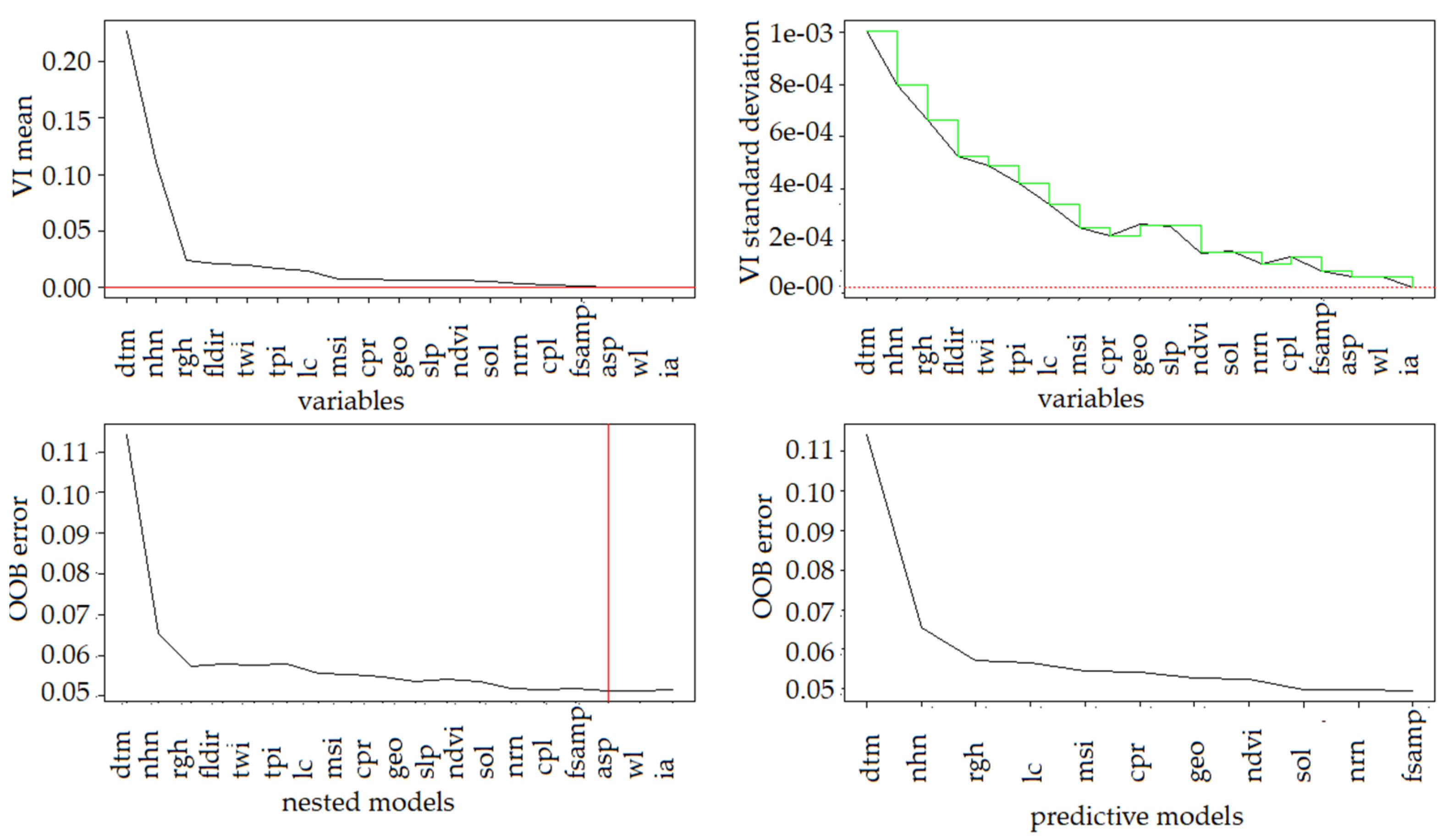
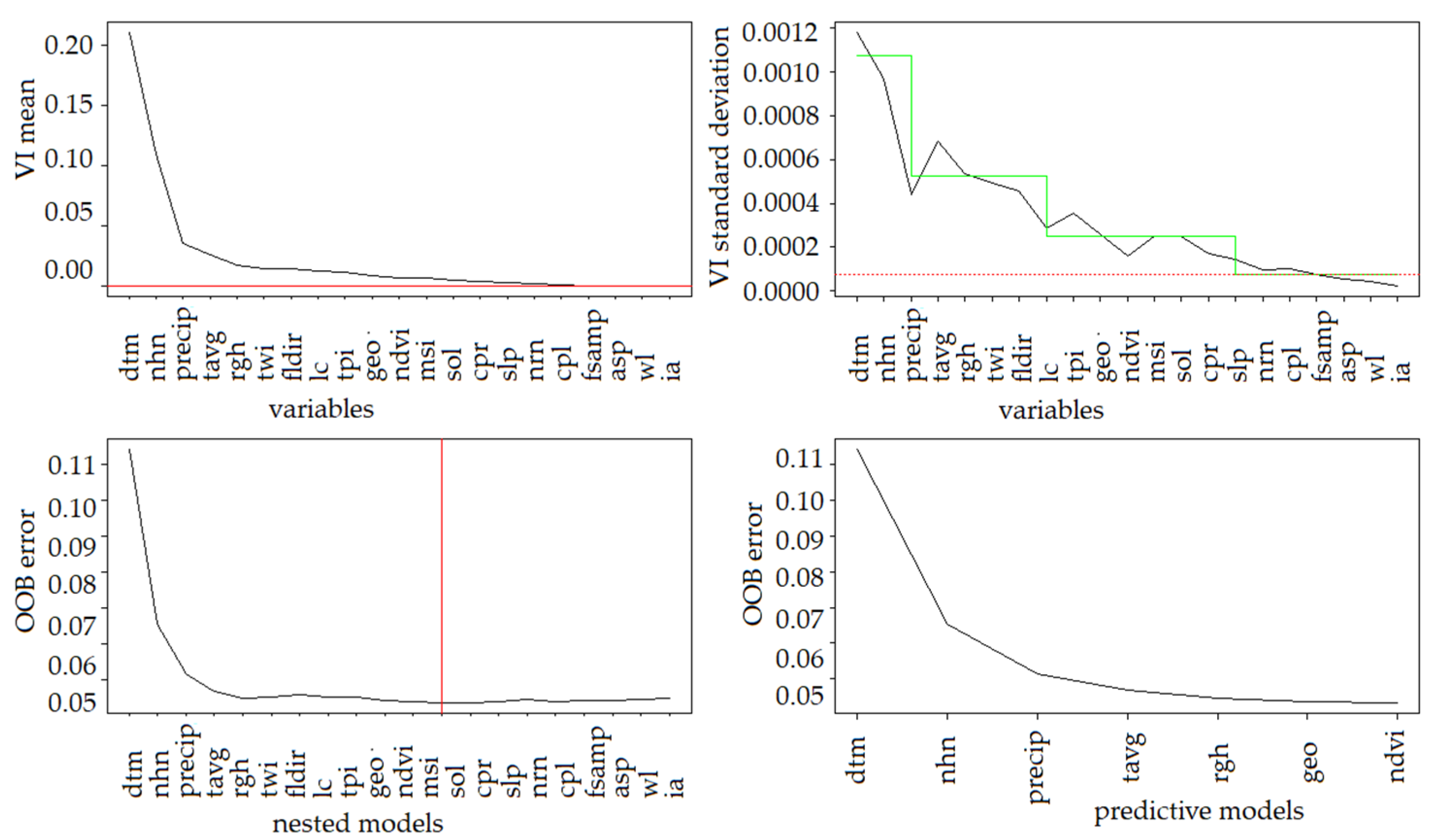
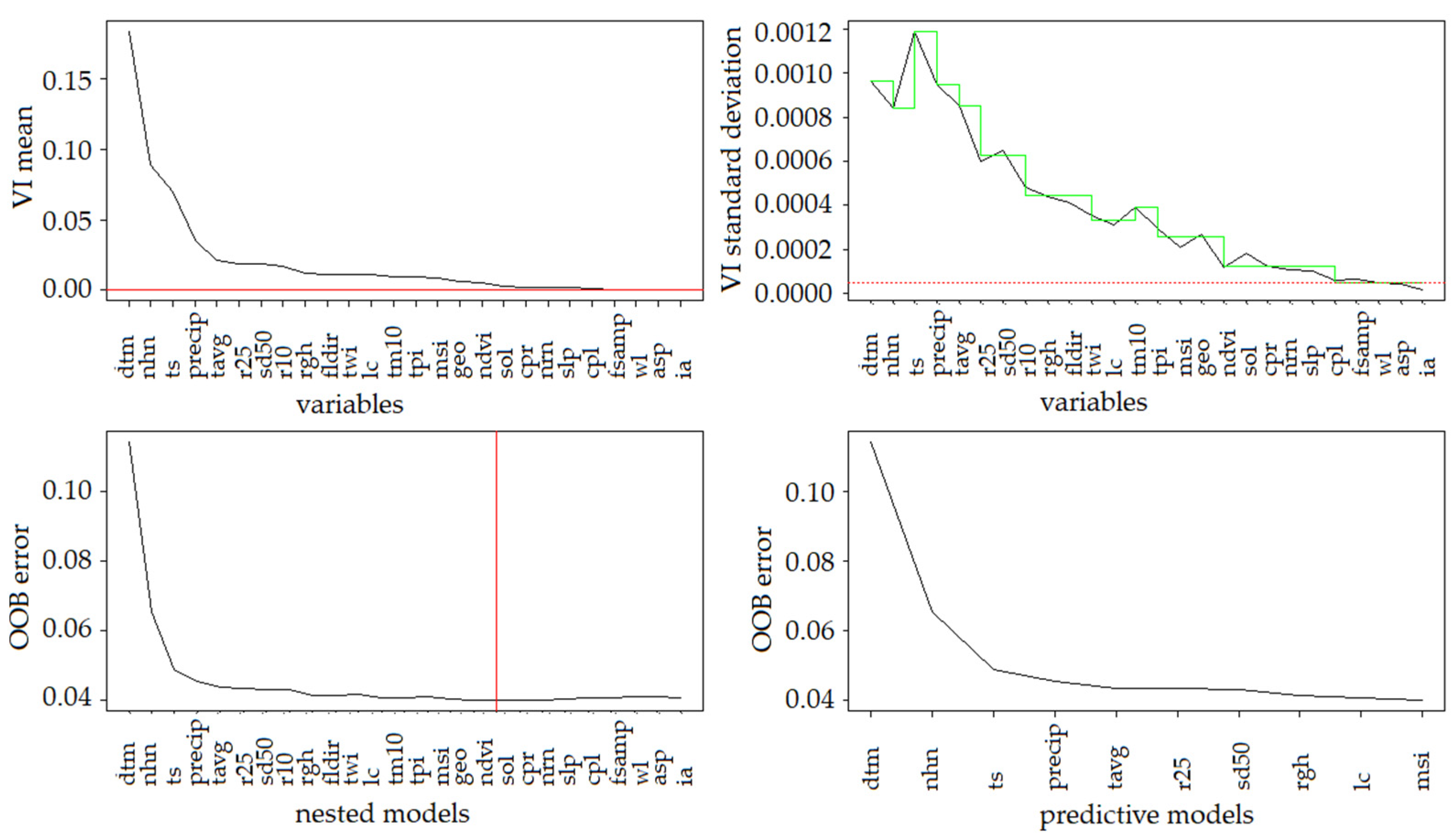
2.3.1. Evaluation of Important Factors

Evaluating the variables that are important for describing the phenomena is a crucial issue. The selection set is limited to those that are supplied. Variable Selection using Random Forest (VSURF) is a three-step variable section using regularized random forest and is best suited for larger datasets [30]. In VSURF hundreds of thousands of decision trees are generated, and the average output of all trees is used to predict an outcome. Each of the tress are derived by performing recursive partitioning of random subsets of the input variables. Variables are selected and the actual cut-points for partitioning is determined based on the goal of splitting data into subsets that have the most differing proportions of the outcome, or information gain. VSURF leverages the variable selection process embedded in random forest and selects the smallest model with an out-of-bag (OOB) error less than the minimal error, augmented by the standard deviation [31]. There are three output variable lists generated: thres, interp and pred; where thres is the full list minus irrelevant variables, interp identifies all variables considered important relative to the response variable based on smallest OOB error, while pred produces a narrower list by eliminating any redundancy in the remaining sub-set of variables for prediction. In this study, those selected by interp were considered those selected by VSURF.

2.3.2. Selected Model

There are a variety of popular ML models available, with many different models showing good performance in flood susceptibility mapping [29]. In various study areas across a wide selection of countries and watersheds, different models have been tested and performed well, with Random Forest being one of those which have performed well. In a study of 179 classifiers from 17 families, [32] found Random Forest to be one of the best classifiers, with the parallel random forest (parRF) providing the best results. They noted that parRF may be considered as a reference (“gold-standard”) to compare with new classifier proposals in order to assess their performance for general classification in general [32]. Other models found to perform very well in their tests were: support vector machine (SVM) avNNet, extreme learning machines with Gaussian kernel and C5.0. The parRF model used in this study was accessed through the R Classification and Regression Training (caret) package [33]. Caret was selected as it provides a set of functions that attempt to streamline the process for creating predictive models, thus, future work testing multiple models can easily be replicated though minimal changes in the code.

Random Forest

Random Forest (RF) classifiers contain a series of individual decision trees that operate as an ensemble. Each individual tree in the RF generates a prediction and the class with the most votes becomes the model prediction, similar to the concept of “wisdom of crowds” [34]. With this approach, a large number of relatively uncorrelated trees operating as a committee will outperform any of the elemental models. To ensure the individual trees are not too correlated, sample with replacement or bagging is used to build the individual trees and node slitting is optimized to produce the greatest separation.
Parallel RF (parRF) as described by [32] optimizes the RF algorithm for use on big data, through hybrid approach that combines data and task parallel optimization. This results in a reduction in processing time and cost, while improving the ability to handle large, noisy and highly dimensional datasets through dimension reduction and a weighted voting approach [35].

2.3.3. Analysis Metrics
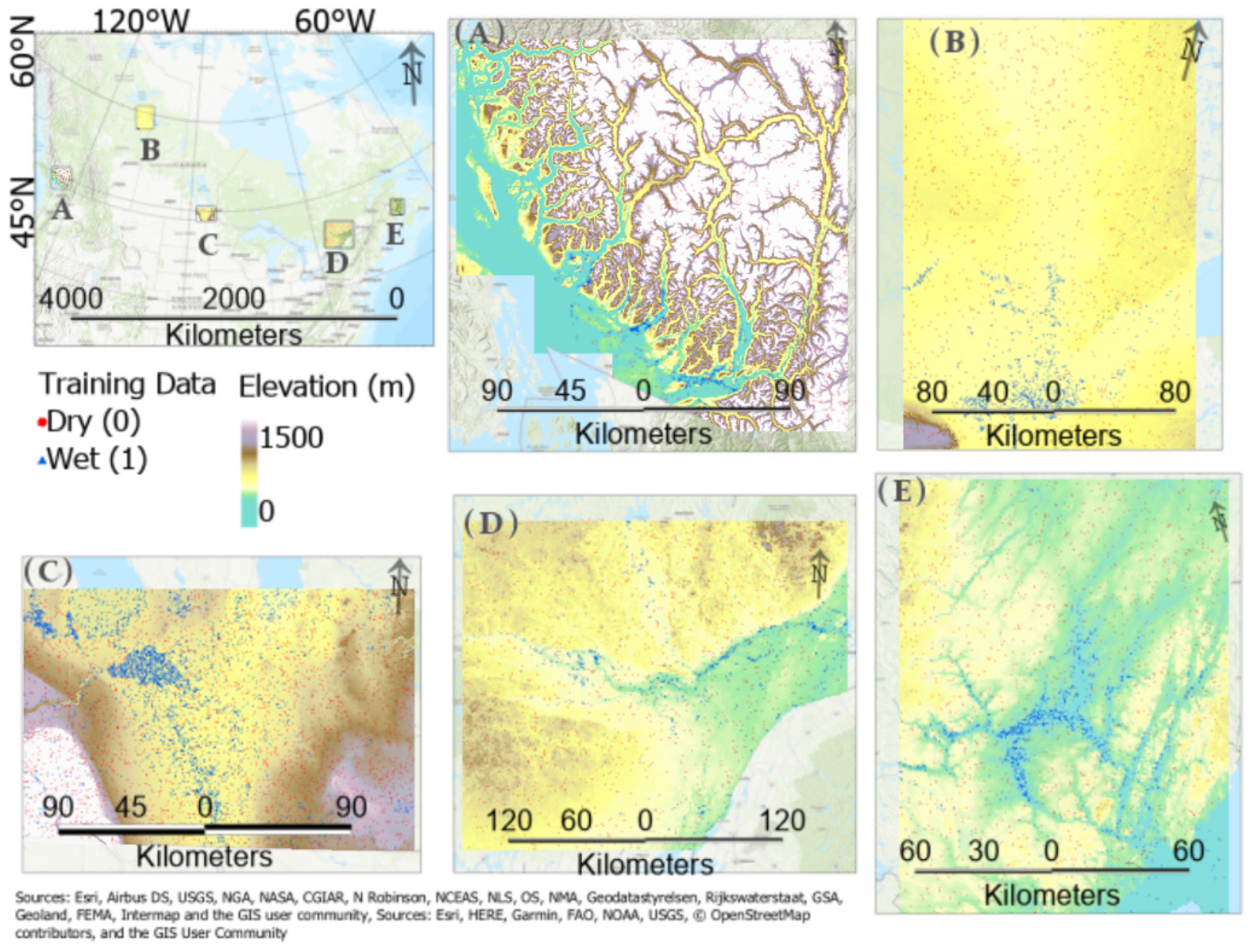
From the literature reviewed, there are a wide variety of metrics used to validate the accuracy of the prediction [10,11,14,15,29]. In this research, Accuracy, ROC, True Skill statistic and F1 were selected to evaluate model performance. Cohen’s kappa coefficient (K), while popular has not been utilized in this research. A shortcoming with K is that while it tries to take away the bias in the actual distribution, evaluation train data gives optimistic results, which may not reflect the model’s performance on unseen data. Cohen’s Kappa, while used in many studies for analysis has not been used in this study, following the recommendation of [36]. Ref. [36] compared Cohens’s Kappa and Matthews Correlation Coefficient (MCC) and found that “when there is a decrease to zero of the entropy of the elements out of the diagonal of the confusion matrix associated with a classifier, the discrepancy between Kappa and MCC rise, pointing to an anomalous performance of the former”.
Accuracy provides a measure of how many points were correctly classified from the confusion matrix, Equation (1):
A c c u r a c y = T P + T N T P + F P + T N + F N
where TP is a true positive, TN is true negative (dry in the reference and dry in the prediction), and FP and FN are incorrectly classified, false positive and false negative, respectively.
The F1 score, a measure of the precision and recall of the classifier is also evaluated:
Precision = T P T P + T N    
Recall = T P T P + F P  
F 1 = ( 1 + β 2 ) P r e c i s i o n   R e c a l l β 2 P r e c i s i o n + R e c a l l
Additionally, the true skill statistic ( T r S k ) is evaluated here. It is defined based on the specificity ( S p ) and sensitivity ( S e ) components of the standard confusion matrix, representing matches and mismatches between observations and predictions [37]:
S p = T P T P + F N
S e = T N F P + T N
T r S k = S p   + S e + 1
Finally, receiver operating characteristic curve (ROC) is generated for validation of the results. A ROC is a graph showing the performance of a classification model at all classification thresholds, plotting the true positive rate versus the false positive rate at different classification thresholds. The Area under the curve (AUC) measures the entire 2-D area underneath the ROC curve, from 0.0 to 1.1.

3. Study Areas

In this study, five study areas in Canada have been selected which have experienced floods in the past 10 years, Figure 2.
The most western study area (BC) surrounds the city of Vancouver. This area is characterized by steep terrain, bedrock geology, with snow-capped mountains, though lower elevation regions rarely experience snow accumulation. This area has the highest average temperature and total precipitation of the selected Canadian study areas. The northern section (AB), which includes a portion of northern Alberta and a southern section of the Northwest Territories, is covered largely with temperate or sub-polar needleleaf forest, relatively flat terrain, and has the coldest average temperatures and the lowest precipitation of the selected study areas. In central Canada, the southern part of Manitoba (MB) was selected, having a long history of flooding, this is an area of flat terrain composed of nutrient rich soils that support significant agricultural crops. The climate is more moderate compared with the AB and BC regions and receives less precipitation. The national capital region (NCR) includes the metropolitan cites of Ottawa, Ontario and Gatineau, Quebec. This area covers the confluence of several waterways including the Ottawa and Gatineau Rivers as they flow into the St. Lawrence River. This study area can be characterized as a large urban, built-up area, surrounded by cropland, forests and hundreds of lakes. It is described by moderate temperature and precipitation, with nearly 4 months of average daily high temperatures above 20 °C and ~3 months of average daily high temperature below 1 °C. The lower portion of the Saint John River in New Brunswick (NB) is the most eastern study area. This area contains Fredericton and St. John as urban centres and Grand Lake and the Grand Lake Meadows Wetland, as well as significant mixed forested areas. In this region the greatest accumulation of snow is found. Several floods have occurred over the past 10+ years, most notably large floods in both 2018 and 2019 that resulted in damage to homes and disruptions to transportation networks, among other impacts [38].

4. Results

4.1. Exploratory Variables
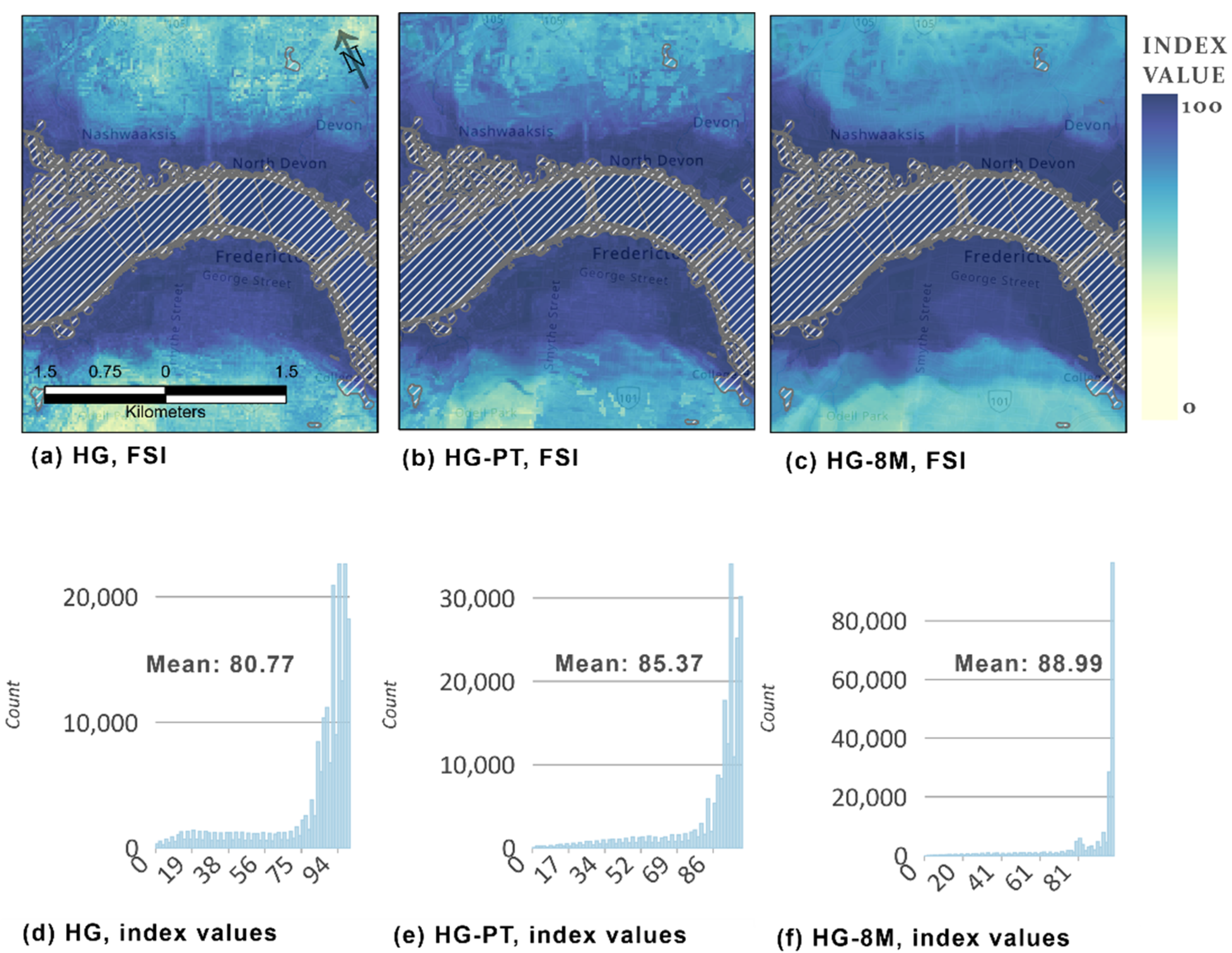
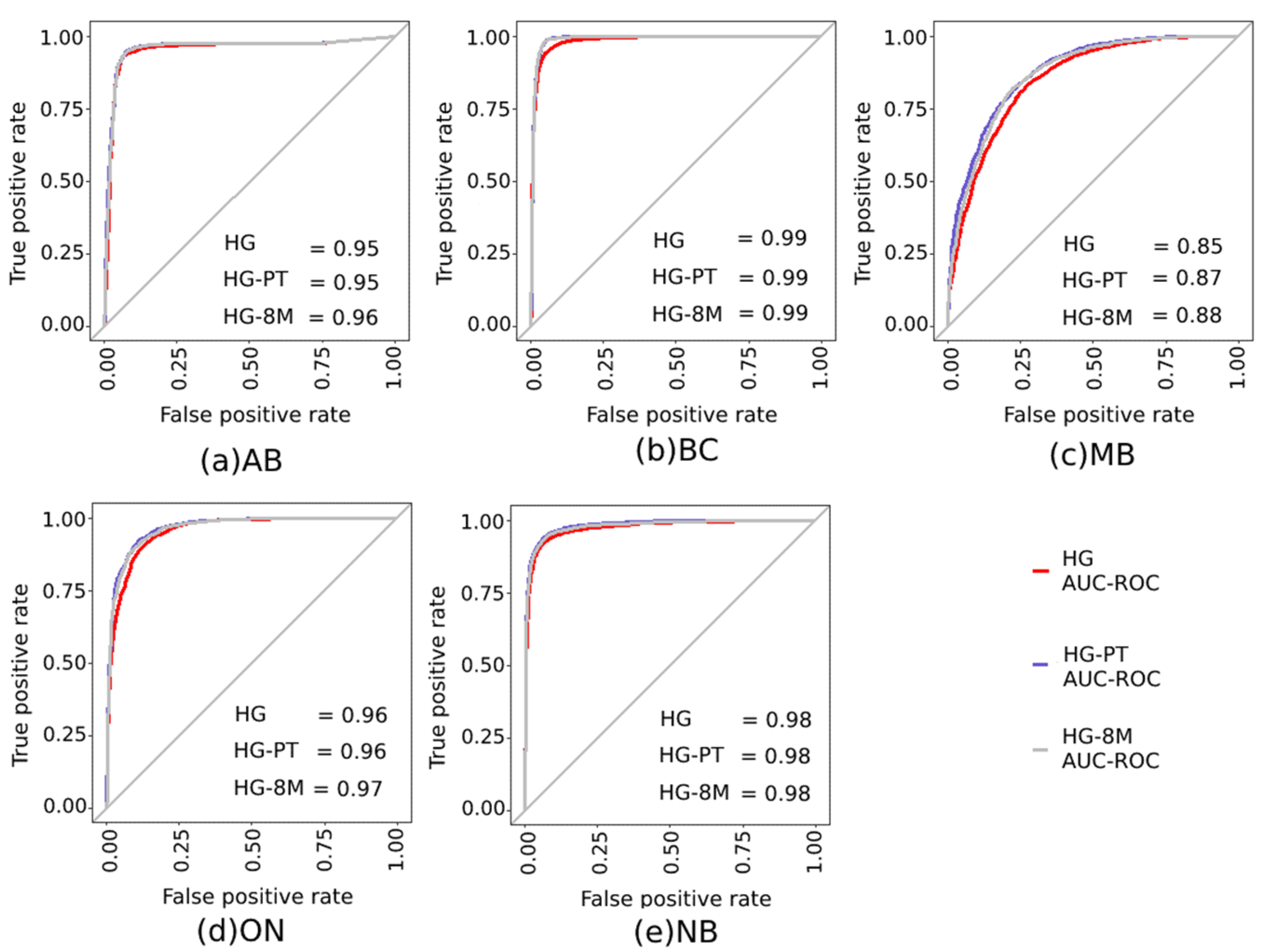
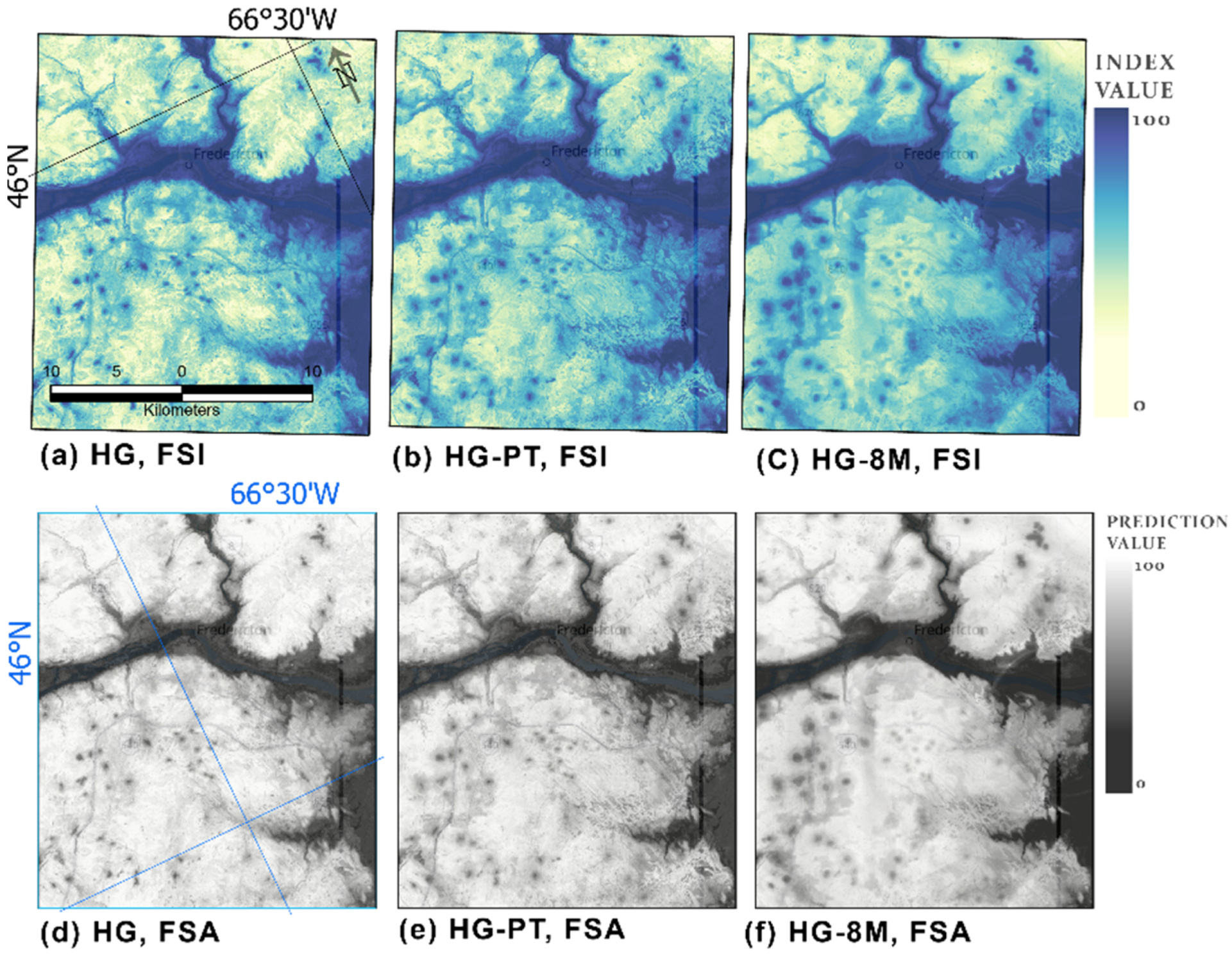
Important variables were tested through three groupings of variables. The results from NB are presented in Figure 3, Figure 4 and Figure 5 for HG, HG-PT and HG-8M, respectively. Equivalent figures for the remaining study areas can be found in the Supplementary Materials. These figures illustrate the mean variable importance and standard deviation of the variable importance in the upper row, while the lower figures display the mean OOB error rate of interpretation step (left) and prediction step (right) of the embedded random forest models.
The HG test included the commonly used variables in flood susceptibility mapping, those that describe the terrain, soil, land cover and hydrography. In all of the study areas, six common variables were retained within the model based on the OOB error rates: dtm, geo, lc, ndvi, nhn and sol, Figure 3. Several other variables were regionally considered important, but not found consistently in all regions.
In HG-PT, for each of the study areas, when precip and tavg were introduced, these variables were considered important in the VSURF test, Figure 4. It is interesting to note that once precip and tavg were added, the overall number of retained variables decreases. In NB, the number of important variables decreases from 10 to 7. Most commonly, the ndvi and sol are dropped from the selection set due to exceeding the OOB error rate, followed by geo, which is dropped in BC, and ON, rgh (dropped from MB and BC), and nrn (AB and NB).
The final test, HG-8M, added several more climate variables not commonly found in flood susceptibility mapping studies, Table 1, Figure 5. An exception is presented by [13], which included frequency of heavy rain, which could be a proxy for the R10 or R25 used in this study. In the HG-8M test, at least three of the eight climate variables were considered important in every study area. The only tested meteorological variable that was absent in the selection set was spr, which represents the number of spring days, March, April, May, with minimum temperatures above 0 °C. In HG-8M, the majority of variables in the selection set were meteorological. All of the sites retained the dtm, lc and nhn variables from the initial HG test.

4.2. Model Results

For each of the study areas, using the optimal variables as determined by VSURF, three ML algorithms were applied to the data. As discussed in Section 2.3.3, the models are evaluated by accuracy, ROC, F1 and true skill ( T r S k ), the results of the parRF model for each study area in Table 2, and Figure 6.
In each of the study areas, the parRF model performs well with regard to the accuracy, true skill and F1 statistic. Of the five study areas, the best results are found in the NB study area and worst in MB. Comparing HG to HG-8M, the parRF model increases from 0.008 to 0.03 in Accuracy, 0.013 to 0.06 in T r S k and 0.006 to 0.038 (F1). The largest improvement from HG to HG-8M is found in the MB study area. Between the HG-PT and HG-8M, there is minor improvements in each of the evaluated metrics. In the ROC curves, there is limited change in between the scenarios tested. The greatest improvement of 0.03 is found in the MB study area.

5. Discussion

The research question considered in this work is why meteorological variables used in engineering flood models are not commonly considered in flood susceptibility studies, and could they improve the performance of ML models if included.
Before the results are discussed, it is important to note that the datasets included cover a range of temporal and spatial scales. The flood events used as training data, primarily range from 2011 to 2020, however, a few significant floods which occurred in the 1970s and 1980s have been included in the training data. Temporal datasets such as land use, wetland, ndvi have been chosen to select 2015 products. Climate data has used the published Normals, with records greater than 15 years over the period of 1980–2010, the most recent period available. The selection of a single year data was thought to not to sufficiently represent the variability of climate, and Normals for 2010–2020 are not available and resources and expertise were not available to generate them. From the available datasets, a 30 m grid was used in many of the geological and ecological datasets and thus was chosen as the resolution for analysis. Downscaling to meet the resolution of the high-resolution terrain data was not appropriate. The authors recognize this variety of time scales and resolutions that were combined in this analysis which may have influence on the presented results.

5.1. Important Factors

In all tests and all study areas, the dtm and nhn layers were considered important variables. These were ranked as either 1 or 2 in order of importance in all study areas, with the exception of MB, where nhn ranked 4th and 8th in the HG and HG-PT tests, respectively. The importance of these variables is expected, given their significance in modelling of floodplain hydrodynamics [39].
When average annual precipitation and temperature, as have been used in several other studies, is included, they are considered an important variable in all five of our study areas. Average annual precipitation and temperature are generally ranked 3rd and 4th in importance, right after the dtm, though in MB and AB, they are ranked 2nd and 3rd, right after the dtm. In three of the five study areas, when precip and tavg are added, the total number of important variables decreases, Table 3, indicating that the addition of these variables produced the most differing proportions of the outcomes.
Several variables found to be important in other studies applying to other regions of the world were not found to be important in these five Canadian study areas: aspect, curvature, both plan and profile, forest cover percentage and wetlands.
Additional meteorological variables, those that capture short-term intense rainfall events, snow coverage and depth, are also considered important and in many cases, more important than traditionally used HG variables Figure 5 (and in Supplementary Materials). In the HG-8M test, at least 3 of the 8 meteorological variables are considered important. Only the spr datasets, which represents the number of spring days with minimum temperature above 0 °C is not considered a significant contributor to flood susceptibility in any of these Canadian study areas. Both snow depth (sd) and Days with min temp < −10 °C (tm10) were found to be important in four of the five study areas.
Surficial geology was found to be important in all but Ontario study area in the HG-8M. This region contains regions of till blanket and till veneer as are found in many of the other regions. However, it largely comprises alluvial sediments along the Ottawa River with regions of offshore and outwash plain sediments. Looking at results of the VSURF test (Supplementary Figure S13), it is surprising that the lc variable passes the OOB error test and geo does not.

5.2. Model Results

While the important factors indicate adding meteorological data, the results of the parRF model shows minor improvements (0.002 to 0.06) in accuracy, true skill, F1, and ROC, Table 2. This suggests that if meteorological factors, relevant to the local environment, are not included in the selection set, then the approach may be missing out on contributing factors to flood susceptibility. As the model is applied to areas not included in the training set, the impact of adding in the meteorological data becomes more apparent. In Figure 7d–f, the prediction accuracy is presented in the NB study area. In Figure 7d, the prediction quality is quite noisy, with many pixels showing an accuracy between 0–50, whereas in Figure 7f, the map presents a larger percentage of pixels with accuracy between 60 and 100.
As the statistical tests showed only minor improvements, the index value of pixels with the historic flood extents boundary were also evaluated, Figure 8. The histogram of pixel values shows a left-skewed distribution in all tests, as is expected. All of the pixels in this polygon extent have the potential to be valued at 100 and could have been part of the training set. The mean value of these pixels increases between HG, HG-PT and HG-8M, with values of 80.77, 85.37 and 88.99, respectively. This provides further evidence supporting the hypothesis to include meteorological datasets, representative of the local environment into the ML model.
The study area with the poorest results was in Manitoba. There are two primary datasets that could potentially explain this decrease in predictive capacity. First, is the limited HRDEM coverage in the area. At the time this analysis was undertaken, this area has the lowest HRDEM coverage, and the majority of the elevation data was therefore derived from the CDEM data. The estimated vertical accuracy of the CDEM in this region is between 0 to 15 m and was validated between 1960 and 1990 [22]. Further to this, the terrain in this region has the smallest elevation relief and it is believed this abundance of CDEM data has attributed to the poorer results. Secondly, this region is largely agricultural, and the national hydrographic dataset does not contain geometry of the agricultural drainage and/or man-made channels that have been excavated to support agricultural fields. The hydrography represents data from 1970 to 1990. Thus, the Euclidean distance raster generated from the hydrographic network likely does not fully represent the try hydrography in the region.

6. Conclusions

In this work, the impact of meteorological factors on the prediction capability of flood susceptibly using ML models has been tested. The standard steps of exploring and evaluating variable importance were first undertaken, then a random forest model was run on five study areas across Canada. These study areas each capture unique characteristics of terrain, geology, land use and climate across the country. Three tests were run: (i) using only hydro-geomorphological (HG) variables; (ii) annual average precipitation and temperature were added (HG-PT), and (iii) including a suite of climate variables including those that capture high-intensity/short duration rainfall, snow accumulation and depth and seasonal norms (HG-8M). The findings illustrate that when adding meteorological variables, their importance outranks many of the traditional datasets that have been tested previously. While the validation metrics of accuracy, true skill, F1 and ROC presented minimal improvements in the prediction capacity, the evaluation of the prediction accuracy and the pixel values with historic flood events further confirmed the assumption that inclusion of meteorological data inputs relative to the local environment improves the resultant flood susceptibility map. Thus, our findings indicate that if some measures of meteorological datasets are not incorporated into flood susceptibility modelling, the approach may not be capturing the full flood susceptibility potential.

Supplementary Materials

The following are available online at https://www.mdpi.com/article/10.3390/rs14071656/s1. Figure S1. AB HG Upper left, mean variable importance, upper right: standard deviation of the variable importance, bottom left: mean OOB error rate of interpretation step of RF models, bottom right: mean OOB error rate of prediction step of RF models. Red lines indicate thresholds, and green line predictions given by a CART tree fitted to standard deviations. Figure S2. AB HG-PT Upper left, mean variable importance, upper right: standard deviation of the variable importance, bottom left: mean OOB error rate of interpretation step of RF models, bottom right: mean OOB error rate of prediction step of RF models. Red lines indicate thresholds, and green line predictions given by a CART tree fitted to standard deviations. Figure S3. AB HG-8M Upper left, mean variable importance, upper right: standard deviation of the variable importance, bottom left: mean OOB error rate of interpretation step of RF models, bottom right: mean OOB error rate of prediction step of RF models. Red lines indicate thresholds, and green line predictions given by a CART tree fitted to standard deviations. Figure S4. BC-HG Upper left, mean variable importance, upper right: standard deviation of the variable importance, bottom left: mean OOB error rate of interpretation step of RF models, bottom right: mean OOB error rate of prediction step of RF models. Red lines indicate thresholds, and green line predictions given by a CART tree fitted to standard deviations. Figure S5 BC HG-PT Upper left, mean variable importance, upper right: standard deviation of the variable importance, bottom left: mean OOB error rate of interpretation step of RF models, bottom right: mean OOB error rate of prediction step of RF models. Red lines indicate thresholds, and green line predictions given by a CART tree fitted to standard deviations. Figure S6. BC HG-8M Upper left, mean variable importance, upper right: standard deviation of the variable importance, bottom left: mean OOB error rate of interpretation step of RF models, bottom right: mean OOB error rate of prediction step of RF models. Red lines indicate thresholds, and green line predictions given by a CART tree fitted to standard deviations. Figure S7. MB-HG Upper left, mean variable importance, upper right: standard deviation of the variable importance, bottom left: mean OOB error rate of interpretation step of RF models, bottom right: mean OOB error rate of prediction step of RF models. Red lines indicate thresholds, and green line predictions given by a CART tree fitted to standard deviations. Figure S8. MB HG-PT Upper left, mean variable importance, upper right: standard deviation of the variable importance, bottom left: mean OOB error rate of interpretation step of RF models, bottom right: mean OOB error rate of prediction step of RF models. Red lines indicate thresholds, and green line predictions given by a CART tree fitted to standard deviations. Figure S9. MB HG-8M Upper left, mean variable importance, upper right: standard deviation of the variable importance, bottom left: mean OOB error rate of interpretation step of RF models, bottom right: mean OOB error rate of prediction step of RF models. Red lines indicate thresholds, and green line predictions given by a CART tree fitted to standard deviations. Figure S10. ON-HG Upper left, mean variable importance, upper right: standard deviation of the variable importance, bottom left: mean OOB error rate of interpretation step of RF models, bottom right: mean OOB error rate of prediction step of RF models. Red lines indicate thresholds, and green line predictions given by a CART tree fitted to standard deviations. Figure S11. ON HG-PT Upper left, mean variable importance, upper right: standard deviation of the variable importance, bottom left: mean OOB error rate of interpretation step of RF models, bottom right: mean OOB error rate of prediction step of RF models. Red lines indicate thresholds, and green line predictions given by a CART tree fitted to standard deviations. Figure S12. ON HG-8M Upper left, mean variable importance, upper right: standard deviation of the variable importance, bottom left: mean OOB error rate of interpretation step of RF models, bottom right: mean OOB error rate of prediction step of RF models. Red lines indicate thresholds, and green line predictions given by a CART tree fitted to standard deviations. Figure S13. Index and estimated accuracy of prediction for the three tested variable groups in the BC study area. Figure S14. Index and estimated accuracy of prediction for the three tested variable groups in the MB study area. Figure S15. Index and estimated accuracy of prediction for the three tested variable groups in the ON/QC study area Figure S16. Index and estimated accuracy of prediction for the three tested variable groups in the AB/NT study area.

Author Contributions

Conceptualization, H.M., methodology, H.M.; software, H.M.; validation, H.M.; formal analysis, H.M.; investigation, H.M.; resources, H.M., P.N.G.; data curation, P.N.G.; writing—original draft preparation, H.M.; writing—review and editing, H.M.; visualization, H.M.; funding acquisition, NRCan, EMS. All authors have read and agreed to the published version of the manuscript.

Funding

This research was funded in part by Natural Resources Canada, Emergency Management Strategy (EMS) fund.

Institutional Review Board Statement

Not applicable.

Informed Consent Statement

Not applicable.

Data Availability Statement

Not applicable.

Acknowledgments

NRCan Contribution number: 20210578. The authors would like to thank Jean-Francois Bourgon, Norah Brown, Marc-Andre Daviault, Jean-Marc Prevost Ryan Ahola and Paula McLeod from CCMEO for their assistance to this work.

Conflicts of Interest

The authors declare no conflict of interest.

References

  1. Natural Resources Canada and Public Safety Canada. Federal Flood Mapping Framework, Technical Report. version 2.0; Government of Canada: Ottawa, ON, Canada, 2018. [Google Scholar]
  2. Coulson, C. Manual of Operational Hydrology in British Columbia; Ministry of Environment, Water Management Division, Hydrology Section: Victoria, BC, Canada, 1991.
  3. Henry, S.; Laroche, A.-M.; Hentati, A.; Boisvert, J. Prioritizing Flood-Prone Areas Using Spatial Data in the Province of New Brunswick, Canada. Geosciences 2020, 10, 478. [Google Scholar] [CrossRef]
  4. Carvalho, A.C.P.; Pejon, O.J.; Collares, E.G. Integration of morphometric attributes and the HAND model for the identification of Flood-Prone Area. Environ. Earth Sci. 2020, 79, 367. [Google Scholar] [CrossRef]
  5. De Lollo, J.A.; Marteli, A.N.; Lorandi, R. Flooding Susceptibility Identification Using the HAND Algorithm Tool Supported by Land Use/Land Cover Data. IAEG/AEG Annu. Meet. Proc. 2018, 2, 107–112. [Google Scholar] [CrossRef]
  6. Echogdali, F.Z.; Boutaleb, S.; Elmouden, A.; Ouchchen, M. Assessing Flood Hazard at River Basin Scale: Comparison between HECRAS-WMS and Flood Hazard Index (FHI) Methods Applied to El Maleh Basin, Morocco. J. Water Resour. Prot. 2018, 10, 957–977. [Google Scholar] [CrossRef] [Green Version]
  7. Khosravi, K.; Shahabi, H.; Pham, B.T.; Adamowski, J.; Shirzadi, A.; Pradhan, B.; Dou, J.; Ly, H.-B.; Gróf, G.; Ho, H.L.; et al. A comparative assessment of flood susceptibility modeling using Multi-Criteria Decision-Making Analysis and Machine Learning Methods. J. Hydrol. 2019, 573, 311–323. [Google Scholar] [CrossRef]
  8. Montani, I.; Marquis, R.; Anthonioz, N.E.; Champod, C. Resolving differing expert opinions. Sci. Justice 2019, 59, 1–8. [Google Scholar] [CrossRef]
  9. Band, S.; Janizadeh, S.; Pal, S.C.; Saha, A.; Chakrabortty, R.; Melesse, A.; Mosavi, A. Flash Flood Susceptibility Modeling Using New Approaches of Hybrid and Ensemble Tree-Based Machine Learning Algorithms. Remote Sens. 2020, 12, 3568. [Google Scholar] [CrossRef]
  10. Alipour, A.; Ahmadalipour, A.; Abbaszadeh, P.; Moradkhani, H. Leveraging machine learning for predicting flash flood damage in the Southeast US. Environ. Res. Lett. 2020, 15, 024011. [Google Scholar] [CrossRef]
  11. Mai, J.; Tolson, B.A.; Shen, H.; Gaborit, É; Fortin, V.; Gasset, N.; Awoye, H.; Stadnyk, T.A.; Fry, L.M.; Bradley, E.A.; et al. Great Lakes Runoff Intercomparison Project Phase 3: Lake Erie (GRIP-E). J. Hydrol. Eng. 2021, 26, 05021020. [Google Scholar] [CrossRef]
  12. Li, X.; Yan, D.; Wang, K.; Weng, B.; Qin, T.; Liu, S. Flood Risk Assessment of Global Watersheds Based on Multiple Machine Learning Models. Water 2019, 11, 1654. [Google Scholar] [CrossRef] [Green Version]
  13. Zhao, G.; Pang, B.; Xu, Z.; Yue, J.; Tu, T. Mapping flood susceptibility in mountainous areas on a national scale in China. Sci. Total Environ. 2018, 615, 1133–1142. [Google Scholar] [CrossRef] [PubMed]
  14. Dodangeh, E.; Choubin, B.; Eigdir, A.N.; Nabipour, N.; Panahi, M.; Shamshirband, S.; Mosavi, A. Integrated machine learning methods with resampling algorithms for flood susceptibility prediction. Sci. Total Environ. 2019, 705, 135983. [Google Scholar] [CrossRef] [PubMed]
  15. Shafizadeh-Moghadam, H.; Valavi, R.; Shahabi, H.; Chapi, K.; Shirzadi, A. Novel forecasting approaches using combination of machine learning and statistical models for flood susceptibility mapping. J. Environ. Manag. 2018, 217, 1–11. [Google Scholar] [CrossRef] [Green Version]
  16. Esfandiari, M.; Abdi, G.; Jabari, S.; McGrath, H.; Coleman, D. Flood Hazard Risk Mapping Using a Pseudo Supervised Random Forest. Remote Sens. 2020, 12, 3206. [Google Scholar] [CrossRef]
  17. Cao, J.; Zhang, Z.; Du, J.; Zhang, L.; Song, Y.; Sun, G. Multi-geohazards susceptibility mapping based on machine learning—a case study in Jiuzhaigou, China. Nat. Hazards 2020, 102, 851–871. [Google Scholar] [CrossRef]
  18. Roopnarine, R.; Opadeyi, J.; Eudoxie, G.; Thongs, G.; Edwards, E. GIS-based flood susceptibility and risk mapping Trinidad using weight factor modeling. Caribb. J. Earth Sci. 2018, 49, 18. [Google Scholar]
  19. Khosravi, K.; Pham, B.T.; Chapi, K.; Shirzadi, A.; Shahabi, H.; Revhaug, I.; Prakash, I.; Bui, D.T. A comparative assessment of decision trees algorithms for flash flood susceptibility modeling at Haraz watershed, northern Iran. Sci. Total Environ. 2018, 627, 744–755. [Google Scholar] [CrossRef] [PubMed]
  20. Arabameri, A.; Saha, S.; Chen, W.; Roy, J.; Pradhan, B.; Bui, D.T. Flash flood susceptibility modelling using functional tree and hybrid ensemble techniques. J. Hydrol. 2020, 587, 125007. [Google Scholar] [CrossRef]
  21. Islam, A.R.M.T.; Talukdar, S.; Mahato, S.; Kundu, S.; Eibek, K.U.; Pham, Q.B.; Kuriqi, A.; Linh, N.T.T. Flood susceptibility modelling using advanced ensemble machine learning models. Geosci. Front. 2020, 12, 101075. [Google Scholar] [CrossRef]
  22. Natural Resources Canada. Map Information Branch. Canadian Digital Elevation Model Product Specifications. 2016. Available online: http://ftp.geogratis.gc.ca/pub/nrcan_rncan/elevation/cdem_mnec/doc/CDEM_product_specs.pdf (accessed on 17 September 2021).
  23. Natural Resources Canada. High Resolution Digital Elevation Model (HRDEM)—CanElevation Series; Product Specifications edition 1.1; Government of Canada: Ottawa, ON, Canada, 2017. [Google Scholar]
  24. R Core Team. R: A Language and Environment for Statistical Computing; R Foundation for Statistical Computing: Vienna, Austria, 2020; Available online: https://www.R-project.org/ (accessed on 1 December 2021).
  25. Latifovic, R. Canada’s Land Cover, Tech. Rep. version 2015; Natural Resources: Ottawa, ON, Canada, 2015. [Google Scholar]
  26. Pearthree, P.A.; Young, J.J.; Cook, J.P. Surficial Geology and Flood Hazards on the Western Piedmont of the Maricopa Mountains and the Southern Piedmont of the Buckeye Hills, Maricopa County, Arizona. 2012. Available online: http://repository.azgs.az.gov/uri_gin/azgs/dlio/1456 (accessed on 27 January 2022).
  27. Hermosilla, T.; Wulder, M.A.; White, J.C.; Coops, N.C.; Hobart, G.W. Disturbance-Informed Annual Land Cover Classification Maps of Canada’s Forested Ecosystems for a 29-Year Landsat Time Series. Can. J. Remote Sens. 2018, 44, 67–87. [Google Scholar] [CrossRef]
  28. Government of Canada. Canadian Climate Normals. Available online: https://climate.weather.gc.ca/climate_normals/ (accessed on 26 August 2021).
  29. Minerva Intelligence and Ebbwater Consulting. National Flood Hazard Data Layer: Schema Design and Implementation Final Report; Minerva Intelligence, Tech. Rep. Project; NRCan—NFHDL: Vancouver, BC, Canada, 2021. [Google Scholar]
  30. Genuer, R.; Poggi, J.-M.; Tuleau-Malot, C. VSURF: An R Package for Variable Selection Using Random Forests. R J. 2015, 7, 19–33. [Google Scholar] [CrossRef] [Green Version]
  31. Sanchez-Pinto, L.N.; Venable, L.R.; Fahrenbach, J.; Churpek, M.M. Comparison of variable selection methods for clinical predictive modeling. Int. J. Med. Inform. 2018, 116, 10–17. [Google Scholar] [CrossRef] [PubMed]
  32. Fernández-Delgado, M.; Cernadas, E.; Barro, S.; Amorim, D. Do we need hundreds of classifiers to solve real world classification problems? J. Mach. Learn. Res. 2014, 15, 3133–3181. [Google Scholar]
  33. Kuhn, M. Caret: Classification and Regression Training; Astrophysics Source Code Library: Leicester, UK, 2021. [Google Scholar]
  34. Bi, J.-W.; Liu, Y.; Fan, Z.-P.; Zhang, J. Wisdom of crowds: Conducting importance-performance analysis (IPA) through online reviews. Tour. Manag. 2018, 70, 460–478. [Google Scholar] [CrossRef]
  35. Chen, J.; Li, K.; Tang, Z.; Bilal, K.; Yu, S.; Weng, C.; Li, K. A Parallel Random Forest Algorithm for Big Data in a Spark Cloud Computing Environment. IEEE Trans. Parallel Distrib. Syst. 2016, 28, 919–933. [Google Scholar] [CrossRef] [Green Version]
  36. Delgado, R.; Tibau, X.-A. Why Cohen’s Kappa should be avoided as performance measure in classification. PLoS ONE 2019, 14, e0222916. [Google Scholar] [CrossRef] [Green Version]
  37. Fielding, A.H.; Bell, J.F. A review of methods for the assessment of prediction errors in conservation presence/absence models. Environ. Conserv. 1997, 24, 38–49. [Google Scholar] [CrossRef]
  38. Mann, R. Recalling the 2018 New Brunswick Floods—One of the Worst in Modern History. Available online: https://www.theweathernetwork.com/ca/news/article/this-day-in-weather-history-april-24-2018-new-brunswick-flooding (accessed on 27 January 2022).
  39. Demir, G.; Akyurek, Z. The Importance of Precise Digital Elevation Models (DEM) in Modelling Floods. In Geophysical Research Abstracts, EGU General Assembly 2016; EGU General Assembly: Vienna, Austria, 2016. [Google Scholar]
Figure 1. Frequency of variables used in flood susceptibility mapping summarized from literature review.
Remotesensing 14 01656 g001
Figure 2. Top-left, overview of study areas the digital terrain model and the training points, (A) British Columbia study (BC), (B) Alberta/Northwest Territories (AB) study area, (C) Manitoba (MB), (D) National Capital Region (NCR) and (E) New Brunswick (NB).
Remotesensing 14 01656 g002
Figure 3. HG variables of importance, NB. Upper left, mean variable importance, upper right: standard deviation of the variable importance, bottom left: mean OOB error rate of interpretation step of RF models, bottom right: mean OOB error rate of prediction step of RF models. Red lines indicate thresholds. The green line represents predictions given by a CART tree fitted to standard deviations.
Remotesensing 14 01656 g003
Figure 4. HG-PT variables of importance, NB. Upper left, mean variable importance, upper right: standard deviation of the variable importance, bottom left: mean OOB error rate of interpretation step of RF models, bottom right: mean OOB error rate of prediction step of RF models. Red lines indicate thresholds. The green line represents predictions given by a CART tree fitted to standard deviations.
Remotesensing 14 01656 g004
Figure 5. HG-8M variables of importance, NB. Upper left, mean variable importance, upper right: standard deviation of the variable importance, bottom left: mean OOB error rate of interpretation step of RF models, bottom right: mean OOB error rate of prediction step of RF models. Red lines indicate thresholds. The green line represents predictions given by a CART tree fitted to standard deviations.
Remotesensing 14 01656 g005
Figure 6. ROC and AUC for each of the five study areas.
Remotesensing 14 01656 g006
Figure 7. Index (ac) and estimated accuracy of prediction (df) for the three tested variable groups in the NB study area.
Remotesensing 14 01656 g007
Figure 8. Distribution of Index pixel values within the boundaries of the Canadian Historic flood event polygon (dissolved polygon of all events on record) from the parRF model.
Remotesensing 14 01656 g008
Table 1. Variables explored in this study. Maps of all study areas and variables can be found in the supplementary data. Datasets are available from open.canada.ca and the universal identifier is indicated. The climate datasets are found on climate-change.canada.ca, CA = specific catchment area, a = local upslope area. Classes: G = geology and ecology, H = hydrography, T = terrain, C = climate, U = urban.
ClassTestVariableCodeSource (UUID from OpenMaps.ca, (Accessed on 17 August 2021))Method
GHGForest Cover (Percent)fcpExtracted from LC
GHGImpermeable AreasiaExtracted from LC
GHGLand Coverlc4e615eae-b90c-420b-adee-2ca35896caf6
GHGNDVIndvi44ced2fa-afcc-47bd-b46e-8596a25e446e
GHGSoilsol0b88062f-ebbe-46c6-ab19-54fd226e9aa7
GHGSurficial Geologygeocebc283f-bae1-4eae-a91f-a26480cd4e4a
HHGFlow DirectionfldirDerivative DTMR raster
HHGMinimum Snow and Icemsi808b84a1-6356-4103-a8e9-db46d5c20fcf
HHGHydrographic networknhna4b190fe-e090-4e6d-881e-b87956c07977
HHGStream Power IndexspiDerivative DTM, NHNln(CA*tan(slp))
HHGTerrain Wetness IndextwiDerivative DTMln(a/tan(slp))
HHGWetlandwl02c992bb-9692-4bff-9517-7a92b09676c7
THGAspectaspDerivative DTMR gdalUtils
THGCurvature-PlancplDerivative DTMR spatialEco
THGCurvature-ProfilecprDerivative DTMR spatialEco
THGDigital Terrain Modeldtm957782bf-847c-4644-a757-e383c0057995, 7f245e4d-76c2-4caa-951a-45d1d2051333
THGRoughnessrghDerivative DTMR gdalUtils
THGSlopeslpDerivative DTMR gdalUtils
THGTerrain Roughness IndextriDerivative DTMR gdalUtils
THGTopographic Position IndextpiDerivative DTMR dalUtils
CHG-PTAverage Precipitationpreciphttps://climate-change.canada.ca/climate-data/#/climate-normals, (accessed on 26 August 2020)R gstat::idw
CHG-PTAverage TemperaturetavgR gstat::idw
C Days with >10 mm Rainfallr10R gstat::idw
CHG-8MDays with >25 mm Rainfallr25R gstat::idw
CHG-8MDays with min temp < −10 °Ctm10R gstat::idw
CHG-8MDays with Snow Depth. 50 cmsd50R gstat::idw
CHG-8MNumber of Spring days, min temp > 0 °CsprR gstat::idw
CHG-8MTotal SnowtsR gstat::idw
UHGEuclidean distance to roadsnrn3d282116-e556-400c-9306-ca1a3cada77f
Table 2. Results of the parRF model for each study area.
parRFAccuracy T r S k F1
SiteHGHG-PTHG-8MHGHG-PTHG-8MHGHG-PTHG-8M
AB0.9530.9550.9570.9040.9110.9140.950.9540.956
BC0.9630.9710.9710.9270.940.940.9630.9690.969
MB0.7970.8220.8270.5930.6430.6530.7820.8110.82
ON0.9030.9230.9260.8050.8450.850.8980.9180.921
NB0.9390.9430.9540.8770.8850.9080.9350.9390.951
Table 3. Summary of important variables, per VSURF Interp, in each of the study areas, viewed by category, HG (hydrographic, terrain and geomorphology) and Meteo for the meteorological variables (temperature, precipitation, snow, etc.).
HGHG-PTHG-8M
HGMeteoTotalHGMeteoTotalHGMeteoTotal
AB707628549
BC9096286511
MB8087298412
ON100106287310
NB120127297512
Publisher’s Note: MDPI stays neutral with regard to jurisdictional claims in published maps and institutional affiliations.

