Ambiguity Resolution for Long Baseline in a Network with BDS-3 Quad-Frequency Ionosphere-Weighted Model

Abstract

For long baseline in a network, the traditional combined ionosphere-free (IF) + wide-lane (WL) strategy is commonly used, but the residual tropospheric delays and larger noise hamper the basic ambiguity resolution (AR). With the completion of the BeiDou global navigation satellite system (BDS-3) and the quad-frequency signals provided by BDS-3 satellites, we can construct more combinations that are conducive to ambiguity resolution. Compared with ionosphere-free linear combinations, we estimated ionospheric delay using three independent WL observations, and formed an ionosphere-weighted model using uncombined code and phase observations, which proved to be quite effective. Based on the real quad-frequency BDS-3 observations of two CORS (Continuously Operating Reference Stations) and two user stations, we processed eight days of data to study the formal and empirical ambiguity success rates and user positioning errors. The rounding success rate of WL ambiguity was significantly improved with ionospheric correction. The success rate of the basic ambiguity increased from 94.4 and 96.1% to 98.0% using the quad-frequency ionosphere-weighted (QFIW) model compared with the double-frequency ionosphere-free (DFIF) model and the triple-frequency geometry-based (TFGB) model. Furthermore, the user E/N/U positioning accuracy improved by 20.6/31.5/13.1% and 6.3/22.9/5.8%, respectively.

1. Introduction

The BeiDou Global Navigation Satellite System (BDS-3) broadcasts five frequency signals, namely B1I, B3I, B1C, B2a, and B2b, centered on 1561.098, 1268.520, 1575.420, 1176.450, and 1207.140 MHz, respectively [1]. Among these signals, B1I, B3I, B1C, and B2a can be received by more civil receivers. This study examines the benefits of these quad-frequency signals with regard to AR for long baseline in a network.

Table 1. Commonly used signals of BDS-2 and BDS-3.

Order Number	Signals		Frequency (MHz)
	BDS-3	BDS-2
1	B1I	B1I	1561.098
2	B3I		1268.520
3	B1C	B3I	1575.420
4	B2a		1176.450
5		B2I	1207.140

shows the commonly used signals of BDS-2 and BDS-3 [1,2].

Multi-frequency observations have significant effects on accelerating ambiguity resolution (AR) and eliminating observation errors such as the ionosphere, and can effectively improve the availability and reliability of RTK positioning. Common multi-frequency AR models include three carrier ambiguity resolution (TCAR) [3,4] and cascading integer resolution (CIR) [5,6]. The basic principles of these two methods are similar. The main idea of TCAR is to fix the ambiguity according to the degree of difficulty. On the basis of selecting the optimal combined observation value of three frequencies, first it fixes the wavelengths of the long extra-wide-lane (EWL) and wide-lane (WL) ambiguities, and finally it fixes the narrow-lane (NL) ambiguity. Common TCAR models include geometry-based (GB), geometry-free (GF), and geometry-ionosphere-free (GIF) models [7,8,9,10].

Early TCAR methods basically used the GF model to solve ambiguity [11,12,13]. Although the GF model will be affected by atmospheric errors, pseudo-range noise, and multipath delays, it is still widely used due to its long wavelength and concise mathematical calculations. The GB model estimates atmospheric error as unknown parameters together with baseline and ambiguity parameters, which greatly improves the strength of the model compared with the GF model. Feng and Li et al. comprehensively analyzed the impact of orbit, ionospheric, and tropospheric errors on the accuracy of combined observations (combined noise). The results showed that even for long baselines, the impact of combined noise on the ambiguity of optimized EWL/WL combinations was basically within 0.2 cycles. However, it is difficult for the GB model to fix the ambiguity of NL [7,11,13]. Gao Wang et al. proposed a network RTK single epoch positioning method based on the BDS three-frequency WL combination. Real-time dynamic positioning is carried out by using the WL observation with fixed ambiguity and minimum noise, and the atmospheric delay correction is obtained by interpolation. The experimental results showed that the success rate of a single epoch model was higher than 99.9%, and the positioning mean error was 3–4 and 5 cm, respectively, for the horizontal and vertical direction [14].

In order to further fix the ambiguity of NL, Li et al. proposed a GIF model using two EWL/WL observations with fixed ambiguity and one NL observation, and estimated the NL ambiguity [13]. However, due to the large model combination coefficient, it was not easy to fix the ambiguity of the narrow lane. Wang et al. added pseudo-range observation to the GIF model and derived a three-frequency combination coefficient of GPS, Galileo, and BDS systems with minimum noise. However, due to the influence of system noise, such as multipath delays, the floating-point solution deviation of basic phase ambiguity was greater than the theoretical derivation result, and hundreds of epochs were needed for smoothing to be less than 0.5 cycles [15]. In addition, Li et al. constructed a GB model using code observations, two EWL observations with fixed ambiguity, and L1 phase observations, and further strengthened the model by imposing constraints on ionospheric and tropospheric parameters. The above models have been verified in ambiguity resolution and high-precision positioning for BDS-2, BDS-3, Galileo, and multi-system GNSS, and have achieved outstanding results [16,17,18].

With the modernization of Galileo and the completion of BDS-3 construction, many scholars have carried out research on fast resolution of quad-frequency or even five-frequency ambiguity. Compared with three-frequency observations, the new frequency point can increase the number of redundant observations and the strength of the positioning model, and theoretically improve the positioning accuracy and robustness [6,19]. Wang et al. used five-frequency Galileo observations, adopted a mathematical model to estimate ionospheric delay with non-combined phase/code observations, and realized the AR of a baseline hundreds of kilometers long under the condition of mitigating the multipath influence. The fixing success rate of three-frequency, quad-frequency, and five-frequency observations was 95, 98, and 99%, respectively, within 10 s smoothing. Therefore, it is proved that quad-frequency or even five-frequency observations provide a certain degree of improvement in the effect of estimating ionospheric delay and AR [19].

Li et al. discussed the advantages of quad-frequency observations, and gave several groups of EWL/WL combination coefficients. Using the observation of ionosphere-free (IF) EWL, dynamic positioning with an accuracy of 0.5 m under a baseline length of 27 km and horizontal positioning accuracy of 1 m under a baseline length of 300 km were achieved. In addition, if the NL observations are used to smooth the IF/EWL combination observations in a short period of time, the positioning error will be reduced to the centimeter level [20]. Most of the research on basic AR using BDS-3 quad-frequency observations are concentrated in the field of PPP [21,22,23].

Ionosphere processing models mainly include ionosphere-fixed, ionosphere-float, ionosphere-free, and ionosphere-weighted models [24]. For sufficiently short baselines, the ionosphere becomes fully correlated. As a result, we can assume that the DD ionospheric delays are known or are absent from the model, which we call the ionosphere-fixed model. However, this assumption is no longer valid when the baseline length increases. For sufficiently long baselines, we can eliminate the influence of ionospheric delays by using the frequency dependent characteristics of the ionosphere through combined dual-frequency or multi-frequency observations, which we call the ionosphere-free model. However, due to the large observation noise, it is generally combined with WL observations to calculate NL ambiguities for positioning. Moreover, we can parameterize the ionosphere in the positioning model to produce an ionosphere-float model that is equivalent to the ionosphere-free model. Therefore, we should try to improve the accuracy of ionosphere information as much as possible to enhance the model strength. For instance, the ionosphere-weighted model is often applied instead of the ionosphere-float model [25].

However, few researchers have comprehensively investigated the benefits of quad-frequency basic AR when the reference stations’ coordinates are precisely known. Hence, in this study, we investigated the aforementioned benefits of quad-frequency signals of BDS-3 in WL AR ionospheric estimation and basic AR in network-based computation.

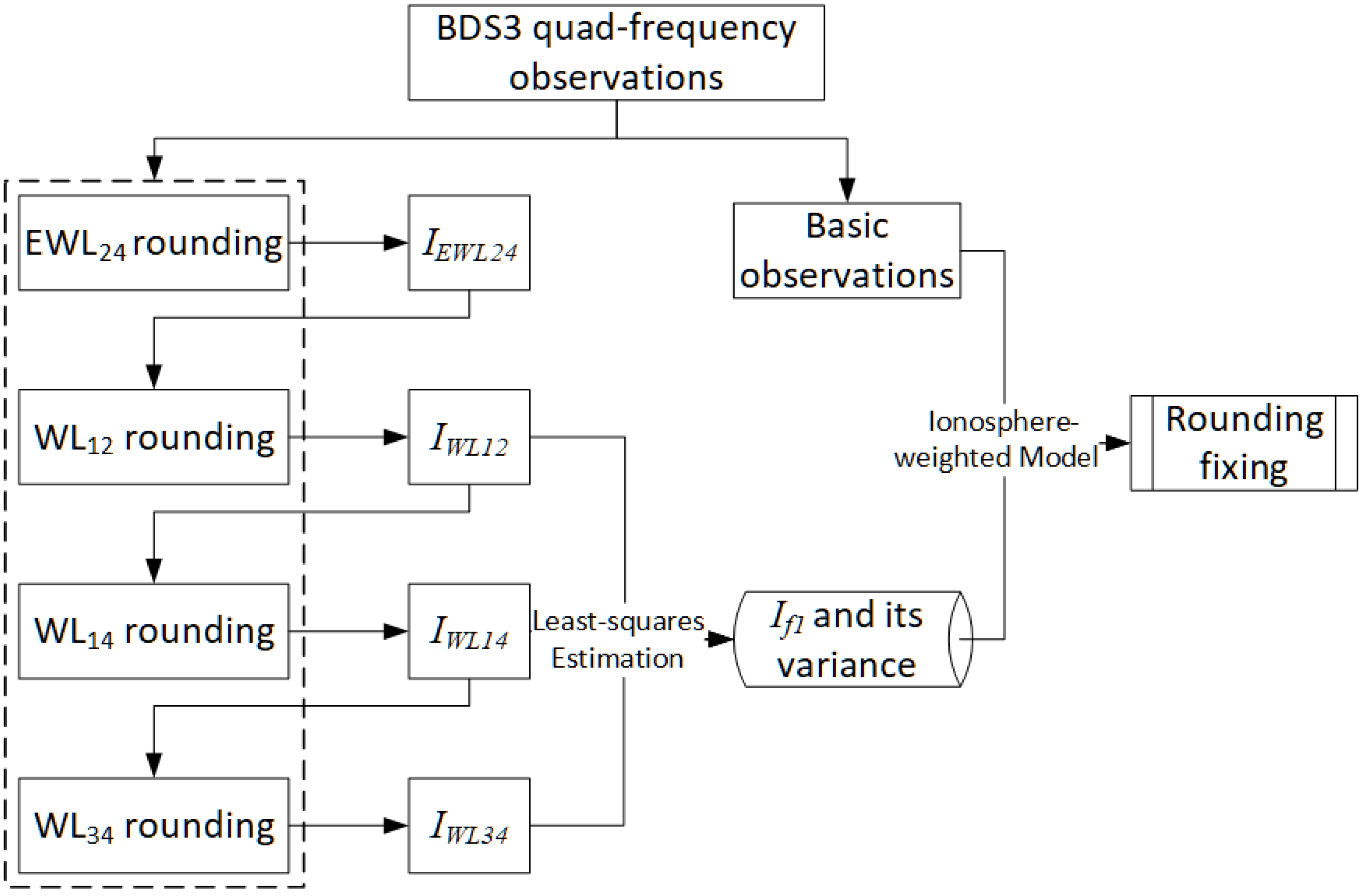
In the following sections, we introduce the general formula of combined multi-frequency observations and give some common combinations of BDS-3 quad-frequency with longer wavelength, less combined noise, or less total noise in cycles. Then, the appropriate EWL/WL combination is selected according to the total noise in cycles and the combined noise coefficient, and the ambiguities of all WL combinations are fixed according to the cascading AR model. In addition, the ionospheric delays are calculated according to three groups of WL observations with fixed ambiguity, and the optimal solution is estimated by least squares. Then, using the ionosphere-weighted model, the floating-point solution of the basic phase ambiguity is estimated by the Kalman filter (KF) and the basic ambiguity is fixed by rounding or the LAMBDA algorithm. Finally, two experiments are conducted to evaluate the performance of quad-frequency basic AR in network-based computation compared with the double-frequency ionosphere-free (DFIF) and triple-frequency geometry-based (TFGB) models [9].

2. Materials and Methods

We begin with the basic observations of BDS multi-frequency signals, then give a description of WL ambiguity resolution step-by-step based on ionosphere correction. Finally, based on quad-frequency observations of BDS-3, the ionosphere-weighted model for basic ambiguity resolution is developed.

2.1. Multi-Frequency Combinations

Multi-frequency observations allow for the formation of more useful combinations, particularly EWL/WL combinations, to enhance AR efficiency. In this section, we first select useful EWL/WL combinations according to the combined wavelength and combined noise.

Satellites $s$ and $r$ are observed by two stations $k$ and $l$ together. By calculating the difference of observations at frequency $f$ of the satellites, the double-differenced (DD) observations between stations and satellites can be obtained.

$$\begin{gathered} \Delta P_{f,kl}^{sr}=\Delta {\rho }_{kl}^{sr}+{\mu }_f\cdot \Delta I_{kl}^{sr}+\Delta T_{kl}^{sr}+\Delta M_{f,kl,p}^{sr}+\Delta e_{f,kl,p}^{sr} \\ \Delta {\varphi }_{f,kl}^{sr}=\Delta {\rho }_{kl}^{sr}-{\mu }_f\cdot \Delta I_{kl}^{sr}+\Delta T_{kl}^{sr}+{\lambda }_f\Delta N_{f,kl}^{sr}+\Delta M_{f,kl,\varphi }^{sr}+\Delta e_{f,kl,\varphi }^{sr} \end{gathered}$$

(1)

In the formula, $\Delta$ represents the double-differenced operator; $P$ and $\varphi$ represent the code and phase observations, respectively; $\rho$ represents the station–satellite distance; $c$ represents the velocity of light; $\mu$ represents the ionospheric delay coefficient; $I$ represents the ionospheric delay; $T$ represents the tropospheric delay; $\lambda$ represents the wavelength of the signal; $N$ represents the DD ambiguity in cycles; $e$ represents the observation noise; and $M_p$ and $M_{\varphi }$ represent the multipath delay of the code and phase, respectively.

Omitting the station and satellite superscripts, the combined observation equations of quad-frequency signals are given as follows:

$$\begin{gathered} \Delta P_{comb}=\Delta \rho +\Delta T+{\eta }_{comb}\Delta I+\Delta M_{P,comb}+\Delta e_{P,comb} \\ \Delta {\varphi }_{comb}=\Delta \rho +\Delta T-{\eta }_{comb}\Delta I+{\lambda }_{comb}\Delta N_{comb}+\Delta M_{\varphi ,comb}+\Delta e_{\varphi ,comb} \end{gathered}$$

(2)

where:

$$\begin{gathered} \Delta {\varphi }_{comb}=\frac{{{\displaystyle \sum }}_{n=1}^4{i}_n\cdot f_n\cdot \Delta {\varphi }_n}{{{\displaystyle \sum }}_{n=1}^4{i}_n\cdot f_n},\Delta P_{comb}=\frac{{{\displaystyle \sum }}_{n=1}^4{i}_n\cdot f_n\cdot \Delta P_n}{{{\displaystyle \sum }}_{n=1}^4{i}_n\cdot f_n} \\ {\lambda }_{comb}=\frac{c}{{{\displaystyle \sum }}_{n=1}^4{i}_n\cdot f_n},\Delta N_{comb}={\displaystyle \sum }_{n=1}^4{i}_n\cdot \Delta N_n,{\eta }_{comb}=\frac{f_1^2({{\displaystyle \sum }}_{n=1}^4{i}_n/f_n)}{{{\displaystyle \sum }}_{n=1}^4{i}_n\cdot f_n} \end{gathered}$$

(3)

Subscript $comb$ represents the quad-frequency combination coefficient $i_1,i_2,i_3,i_4$, and they are all integers, and other symbols have the same meaning as in Formula (1). In this study, we selected useful quad-frequency combinations for AR based on the total noise level relative to the combined wavelength in cycles, the combined wavelength, and the combined noise. The total noise is combined with ionospheric and tropospheric delays and phase noises, as follows:

$${\sigma }_{comb}=\sqrt{{\delta }_T^2+{\eta }_{comb}^2{\delta }_I^2+{\sigma }_{{\varphi }_{comb}}^2}/{\lambda }_{comb}$$

(4)

where ${\sigma }_{comb}$ represents the total noise in cycles, and ${\delta }_T$ and ${\delta }_I$ represent tropospheric and ionospheric delay, respectively. Supposing that the accuracy of the quad-frequency phase observations is the same, i.e., ${\sigma }_{{\varphi }_1}={\sigma }_{{\varphi }_2}={\sigma }_{{\varphi }_3}={\sigma }_{{\varphi }_4}={\sigma }_{\varphi }$, the combination phase noise can be written as: ${\sigma }_{{\varphi }_{comb}}^2=\frac{{{\displaystyle \sum }}_{n=1}^4{(i_n\cdot f_n)}^2}{{({{\displaystyle \sum }}_{n=1}^4{i}_n\cdot f_n)}^2}{\sigma }_{\varphi }^2={\mu }_{comb}^2{\sigma }_{\varphi }^2$, where $\mu$ is the multiplier factor of the phase noise.

Based on the empirical value of ionospheric delays, tropospheric delays, and phase noises, we calculated the total noise level of the combined observations, and some commonly used combinations of EWL and WL are shown in

Table 2. Total noise level for commonly used combinations under different error budgets.

Combinations	${\mathit{\lambda }}_{\mathit{c}\mathit{o}\mathit{m}\mathit{b}}\left(\mathbf{m}\right)$	${\mathit{\mu }}_{\mathit{c}\mathit{o}\mathit{m}\mathit{b}}$	${\mathit{\eta }}_{\mathit{c}\mathit{o}\mathit{m}\mathit{b}}$	Total Noise Level (Cycles)
				${\mathit{\delta }}_{\mathit{I}}=10\mathbf{cm}$	${\mathit{\delta }}_{\mathit{I}}=20\mathbf{cm}$	${\mathit{\delta }}_{\mathit{I}}=80\mathbf{cm}$
				${\mathit{\delta }}_{\mathit{T}}=5\mathbf{cm}$	${\mathit{\delta }}_{\mathit{T}}=10\mathbf{cm}$	${\mathit{\delta }}_{\mathit{T}}=15\mathbf{cm}$
(−1, 0, 1, 0)	20.9323	154.858	−0.991	0.037	0.038	0.053
(0, 1, 0, −1)	3.256	18.791	−1.633	0.060	0.109	0.405
(4, −3, −3, 2)	4.579	137.759	−0.261	0.151	0.152	0.161
(1, −3, 0, 2)	2.765	43.700	−0.558	0.084	0.096	0.188
(1, −1, 0, 0)	1.025	6.875	−1.231	0.134	0.261	0.972
(0, −1, 1, 0)	0.977	6.591	−1.219	0.139	0.272	1.010
(1, 0, 0, −1)	0.779	5.082	−1.327	0.185	0.366	1.377
(0, 0, 1, −1)	0.751	4.928	−1.315	0.190	0.376	1.415

. Table 2 also shows the combined wavelengths and combined phase noises of several EWL/WL combinations under various given error budgets. The basic phase observation noise was set to 5 mm at all frequencies. For each error budget, three linearly independent combinations with the lowest total noise level are shown in bold.

It can be seen from Table 2 that EWL combination (−1, 0, 1, 0) has a total noise level that is less than 0.1 cycles under all error budgets because it has the longest wavelength. At the same time, EWL combinations (1, −3, 0, 2) and (4, −3, −3, 2) also performed well under all error budgets, with a total noise level of less than 0.2 cycles. Although these EWL combinations have small total noise levels in cycles, because of the large, combined noise, the calculated ionospheric delay cannot meet the accuracy requirements. EWL combination (0, 1, 0, −1) performed better under low ionospheric biases, and the total noise level reached 0.4 cycles under high ionospheric biases, but the high fixing success rate of AR could still be achieved with observation smoothing. At the same time, the combination (0, 1, 0, −1) has the smallest ${\mu }_{comb}$ among all EWL combinations listed in the table, allowing ionospheric delay to be calculated with higher precision.

Based on Formula (2), we can calculate ionospheric delay using EWL/WL observations, as shown in Formula (5). It can be seen from the formula that the calculated ionospheric delay is mainly affected by residual tropospheric delay, multipath delay, and combined observation noise. Among them, tropospheric delay is corrected by the empirical model and the residual error is small. Reference stations are mostly built in open areas and are less affected by the multipath phenomenon. Therefore, both errors can be ignored. Furthermore, the combined observation noise can be weakened by three linearly independent WL combinations. The estimated ionosphere delay can be used for the basic phase AR.

$$\Delta I=(\Delta \rho -\Delta {\varphi }_{comb}+\Delta {\lambda }_{comb}\Delta N_{comb}+\Delta T+\Delta M_{comb}+\Delta e_{comb})/{\eta }_{comb}$$

(5)

2.2. Ionospheric Estimation and Basic Ambiguity Resolution

The combined phases ${\varphi }_{(0,1,0,-1)}$ (referred to as EWL₂₄) are used to estimate the approximate value of ionospheric delay $I_{EW{L}_{24}}$, but the accuracy of $I_{EW{L}_{24}}$ is poor and it cannot be used directly for basic ambiguity fixing due to the large noise. Based on the idea of cascading AR, $I_{EW{L}_{24}}$ is brought into the equation of WL phases ${\varphi }_{(1,-1,0,0)}$ (referred to as WL₁₂) to improve the accuracy of its floating-point solution. After ambiguity fixing by rounding, a more accurate ionospheric delay $I_{W{L}_{12}}$ is calculated. The same method is used to fix the ambiguities of WL phases ${\varphi }_{(1,0,0,-1)}$ (WL₁₄) and ${\varphi }_{(0,0,1,-1)}$ (WL₃₄), and the corresponding ionospheric delays $I_{W{L}_{14}}$ and $I_{W{L}_{34}}$ are calculated. Finally, the ionosphere delay $I_{f_1}^s$ of satellite $s$ is calculated by using least-squares estimation (LSE) with Formula (6). The algorithmic process is shown in Figure 1.

$$\left[\begin{array}{c}{I}_{W{L}_{12}}^s\\ I_{W{L}_{14}}^s\\ I_{W{L}_{34}}^s\end{array}\right]=\left[\begin{array}{c}{\eta }_{W{L}_{12}}\\ {\eta }_{W{L}_{14}}\\ {\eta }_{W{L}_{34}}\end{array}\right]I_{f_1}^s,Q_{WL}=diag({\sigma }_{W{L}_{12}}^2,{\sigma }_{W{L}_{14}}^2,{\sigma }_{W{L}_{34}}^2),$$

(6)

where $Q_{WL}$ is the covariance matrix of ionospheric delays calculated by WL observations, and the other symbols have the same meanings as in Formulas (3) and (4). The ionospheric estimation is $I_{f_1}^s={({\eta }^T{Q}_{WL}^{-1}\eta )}^{-1}{\eta }^T{Q}_{WL}^{-1}{I}_{WL}$, and the variance of the ionospheric estimation is $Q_I={({\eta }^T{Q}_{WL}^{-1}\eta )}^{-1}$, where $I_{WL}={[\begin{array}{ccc}{I}_{W{L}_{12}}^s& I_{W{L}_{14}}^s& I_{W{L}_{34}}^s\end{array}]}^T$, $\eta ={[\begin{array}{ccc}{\eta }_{W{L}_{12}}& {\eta }_{W{L}_{14}}& {\eta }_{W{L}_{34}}\end{array}]}^T$.

While the ionosphere delays and their variances are estimated by Formula (6), we can use the ionosphere-weighted model to estimate the basic ambiguity, which we call the quad-frequency ionosphere-weighted model (QFIW). The uncombined DD observation equations of quad-frequency signals are as follows:

$$E\left[\begin{array}{c}\overline{p}\\ \overline{\varphi }\\ x\\ \overline{\iota }\end{array}\right]=\left[\begin{array}{ccccc}{e}_4\otimes A& \eta \otimes I_s& 0& 0& 0\\ e_4\otimes A& \eta \otimes I_s& \mathsf{\Lambda }\otimes I_s& 0& 0\\ 0& 0& 0& 1& 0\\ 0& 0& 0& 0& 1\end{array}\right]\left[\begin{array}{c}x\\ \overline{\iota }\\ z\\ \widehat{X}\\ \widehat{I}\end{array}\right]$$

(7)

where $\overline{p}$ and $\overline{\varphi }$ represent the quad-frequency DD observations of the code and phase, respectively; $\overline{\iota }$ represents the DD ionospheric parameter vector; $A$ is the design matrix for parameters $x$ consisting of three coordinates ${\left[\begin{array}{ccc}\Delta x& \Delta y& \Delta z\end{array}\right]}^T$; $\eta ={\left[\begin{array}{cccc}{\eta }_1& {\eta }_2& {\eta }_3& {\eta }_4\end{array}\right]}^T$ is the scalar vector for the DD ionosphere parameters; $\mathsf{\Lambda }=diag({\lambda }_1,{\lambda }_2,{\lambda }_3,{\lambda }_4)$ denotes the quad-frequency wavelengths; $z={\left[\begin{array}{cccc}{z}_1^T& z_2^T& z_3^T& z_4^T\end{array}\right]}^T$ denotes the quad-frequency DD ambiguities; $\widehat{X}={\left[\begin{array}{ccc}\widehat{x}& \widehat{y}& \widehat{z}\end{array}\right]}^T$ denotes the known coordinates of the baseline; $\widehat{I}={\left[\begin{array}{ccc}{\widehat{I}}_{{}^{f_1}}^1& \cdots & {\widehat{I}}_{{}^{f_1}}^s\end{array}\right]}^T$ denotes the ionospheric delays estimated by Formula (6); $e_4$ is a four-column vector in which all elements are 1; and $I_s$ is an identity matrix with dimension $s$. The covariance matrix of the DD observations is given as follows:

$$Q_{DD}=diag(Q_p,Q_{\varphi },Q_{\widehat{X}},Q_{\widehat{I}})$$

(8)

where $Q_p={\sigma }_p^2\otimes I_4\otimes P^{-1}$ is the covariance matrix of code, $Q_{\varphi }={\sigma }_{\varphi }^2\otimes I_4\otimes P^{-1}$ is the covariance matrix of phase, $Q_{\widehat{X}}=diag({0.1}^2,{0.1}^2,{0.1}^2)$ is the covariance matrix of known coordinates; $Q_{\widehat{I}}=Q_I\otimes P^{-1}$ is the covariance matrix of estimated ionosphere; $P=Q^{-1}$ is the DD weight matrix; and $Q$ is the corresponding co-factor matrix calculated by the elevation weighting model.

Utilizing the above model, when the ambiguity accuracy and deviation are obtained, the a priori success rate of ambiguity rounding fixing can be calculated according to Equation (9). In this study, we assumed that the residual tropospheric delays and multipath delays were systematic error $\delta$ and the observation noise was random error $\sigma$. At the same time, assuming that the observation accuracy of DD phase is ${\sigma }_{\varphi }$ = 3 mm and ${\sigma }_{\varphi }$ = 5 mm, the ambiguity rounding success rates of the DFIF and QFIW models under different system errors are calculated by Equation (9):

$$P(-0.5<x<0.5)={\displaystyle \underset{-0.5}{\overset{+0.5}{\int }}\frac{1}{\sigma \sqrt{2\pi }}\exp (-\frac{{(x-\delta )}^2}{2{\sigma }^2})}dx$$

(9)

The rounding fixing success rates of the two models are shown in Figure 2. It can be seen from the figure that when ${\sigma }_{\varphi }$ = 3 mm, the QFIW model could maintain a 100% success rate when the system error was less than 7 cm, while the DFIF model produced wrong fixing when the system error was greater than 2 cm. When ${\sigma }_{\varphi }$ = 5 mm, the QFIW model could maintain a 100% success rate when the system error was less than 5 cm, while the DFIF model always had the possibility of producing wrong fixing. Under all noise budgets, the QFIW model had a higher ambiguity fixing success rate than the DFIF model. From the aspect of the a priori success rate of AR, we proved the advantages of the QFIW model for AR between reference stations proposed in this study.

3. Results

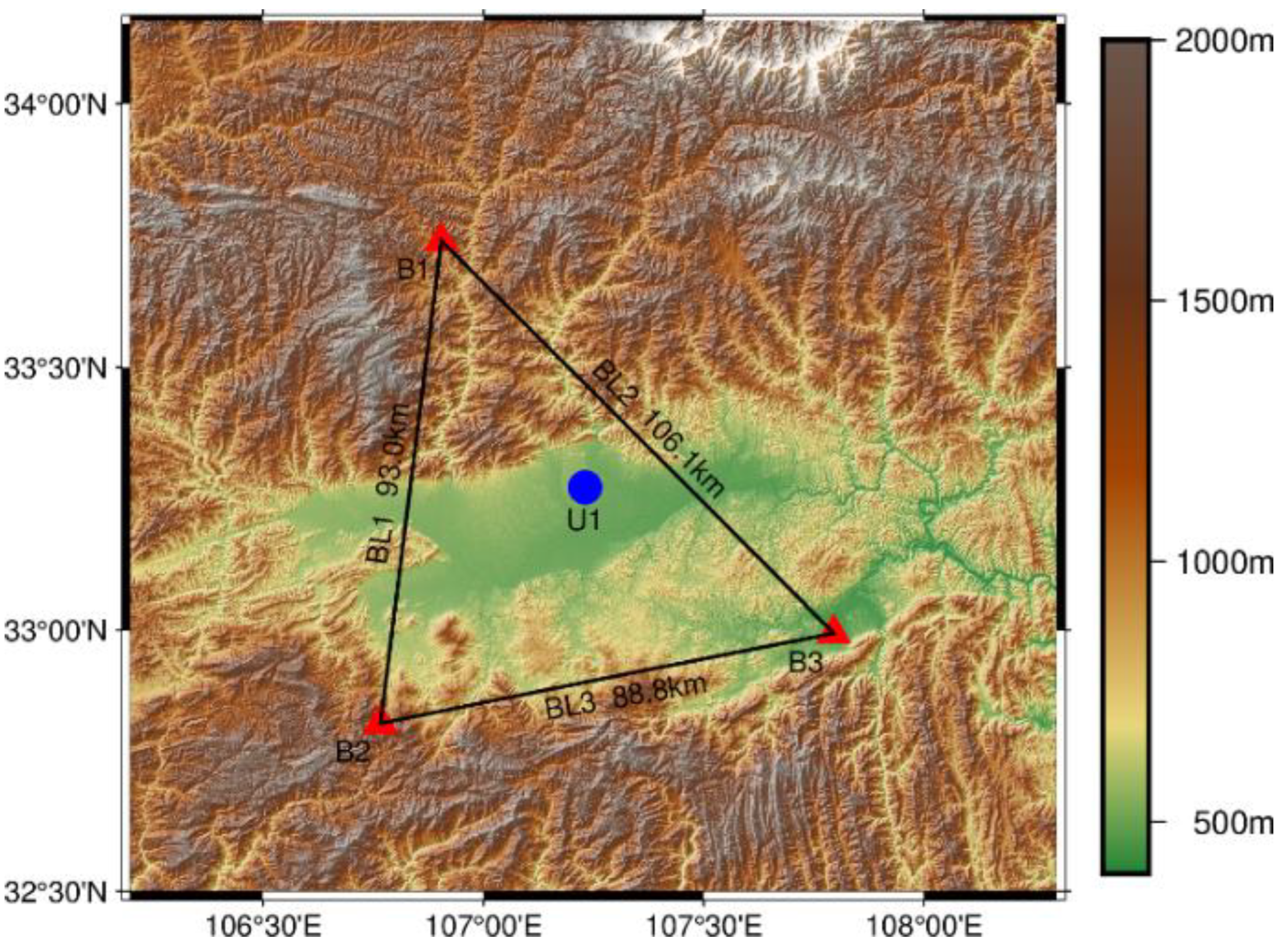
Two CORS (Continuously Operating Reference Stations), each consisting of three reference stations and one user station, distributed around 33°N, 107°E and 32°N, 119°E, respectively, were used for processing. BDS-3 observations of all eight stations were processed on four frequencies. The two CORS are distributed in central China, for long baselines in other regions; the biggest difference is the number of BDS satellites. In this paper we mainly studied the advantages of quad-frequency observations in ambiguity resolution and positioning accuracy compared with double-frequency observations, so the number of satellites does not have a substantial impact on the conclusions.

For the first CORS network, the base stations and user station had the same types of receivers and antennas—Trimble Alloy receivers and TRM159900.00 SCIS antennas. The average length of three baselines is close to 100 km, and the maximum height difference between base stations is up to 1000 m. Observations of day of year (DOY) 148 in 2020 were used for experimental verification in this study. The elevation mask was set to 10°, and the sample rate was 30 s. Figure 3 displays the geographical location of the stations. The broadcast ephemerides were used to assess the satellite ORTs in real time. The tropospheric delay was mitigated by an empirical model, saastamoinen + GPT2_1w. The receiver antenna phase offset was ignored, as the same antenna type was used. The quad-frequency DD algorithm was used in the data processing, and the ambiguities of each epoch were resolved by Kalman filter. With all ambiguities resolved, accurate tropospheric and ionospheric delays of each baseline could be calculated, which were then used to interpolate the atmospheric delay at the user’s position and finally generate virtual observations.

Three groups of BDS-3 network RTK solutions were compared: DFIF, TFGB, and QFIW. We compared the fixing success rate of WL and basic ambiguities, the number of successfully fixed satellites, and the user-side positioning accuracy of the two methods, as follows.

The accuracy of the float WL ambiguity directly determines the success rate of the WL ambiguity resolution, and it has a great impact on both the double-frequency and quad-frequency solution. We followed the idea of cascading AR. First, the EWL₂₄ ambiguities were fixed, and the ionospheric delay $I_{EW{L}_{24}}$ was calculated according to Equation (5). It can be seen from Table 2 that the fixing success rate of rounding was almost 100%. Then, the ionospheric delay $I_{EW{L}_{24}}$ was used as a constraint equation to improve the accuracy of WL₁₂ floating ambiguities. Finally, the fixed WL₁₂ ambiguities were used to calculate the higher-precision ionospheric delay $I_{W{L}_{12}}$, which in turn fixed the WL₁₄ and WL₃₄ ambiguities according to the above method.

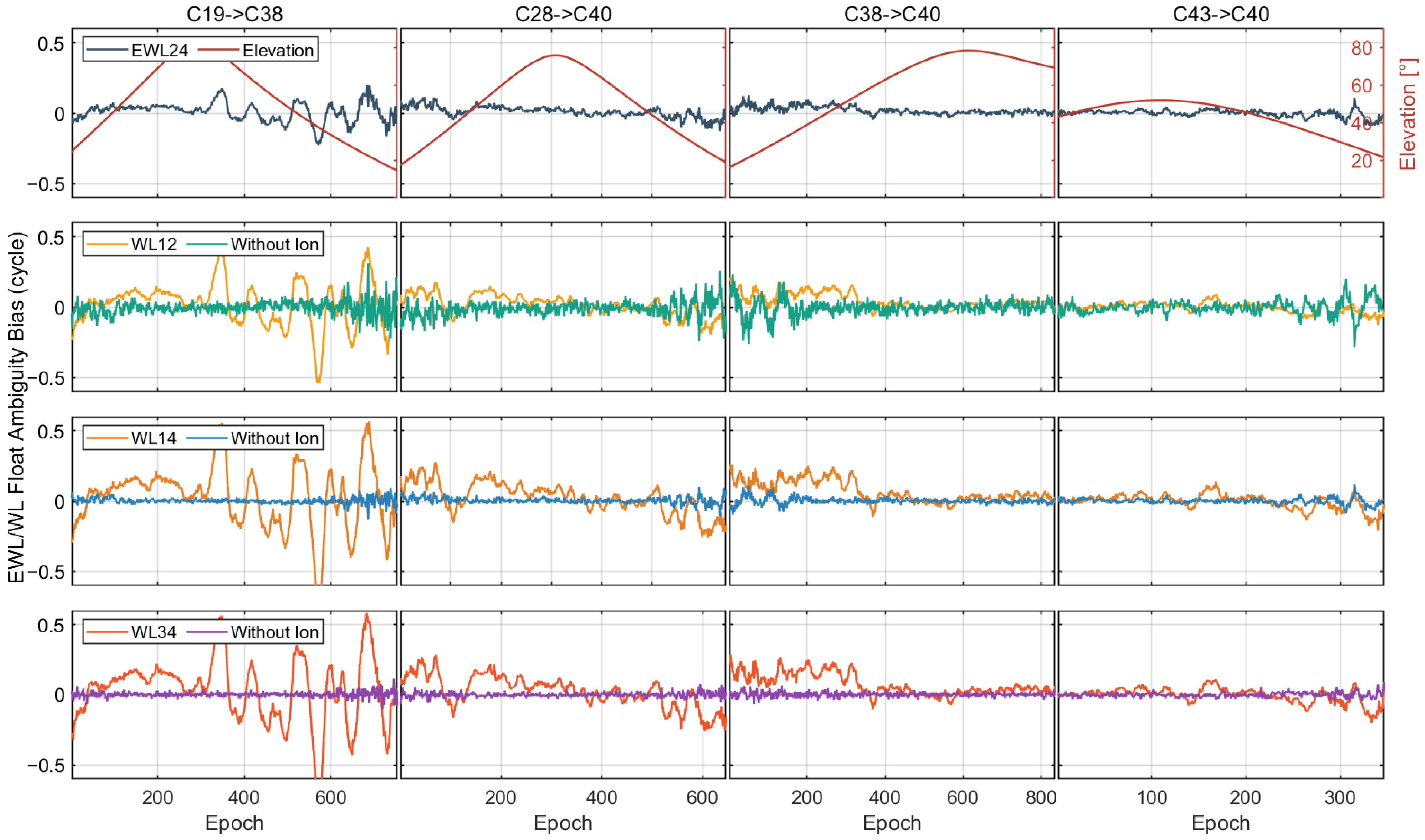
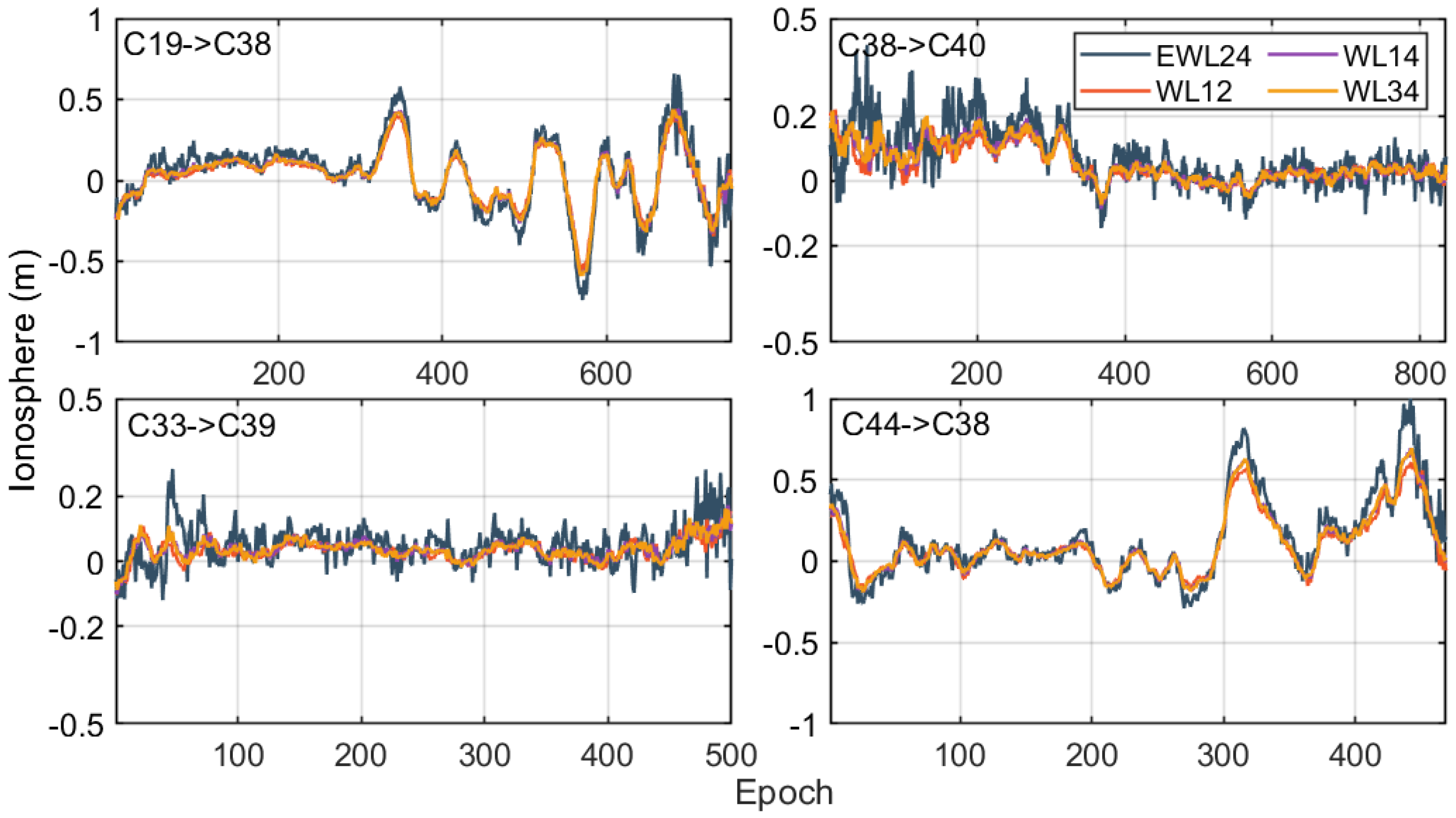
We selected four sets of satellite pairs (C19-C38, C28-C40, C38-C40, and C43-C40) to compare the accuracy of the WL float ambiguities before and after ionospheric correction. It can be seen from Equation (2) that the floating solution bias mainly included ionospheric delay, tropospheric model errors (mainly wet delay), and multipath delay, among which ionospheric delay has the greatest influence. Therefore, the WL floating ambiguities after ionospheric correction were basically close to integers.

Figure 4 shows the float ambiguity biases of EWL and WL combinations. As shown in the figure, all EWL ambiguities could be fixed correctly, benefiting from the long wavelength. In addition, the WL float ambiguity bias of some satellites exceeds 0.5 cycles, indicating that direct rounding will cause this part of the ambiguity to be fixed incorrectly. This will also cause errors in the basic ambiguity resolution. In contrast, the bias of the WL float solution after ionospheric correction was basically within 0.2 cycles, which can effectively ensure the success rate of WL ambiguity resolution by rounding. The WL float solution bias after ionospheric correction was close to white noise, and the fluctuation at a low altitude angle was mainly caused by residual tropospheric wet delays and multipath delays. It can also be seen from Figure 4 that the noise of combinations WL₁₄ and WL₃₄ were equivalent and smaller than that of WL₁₂.

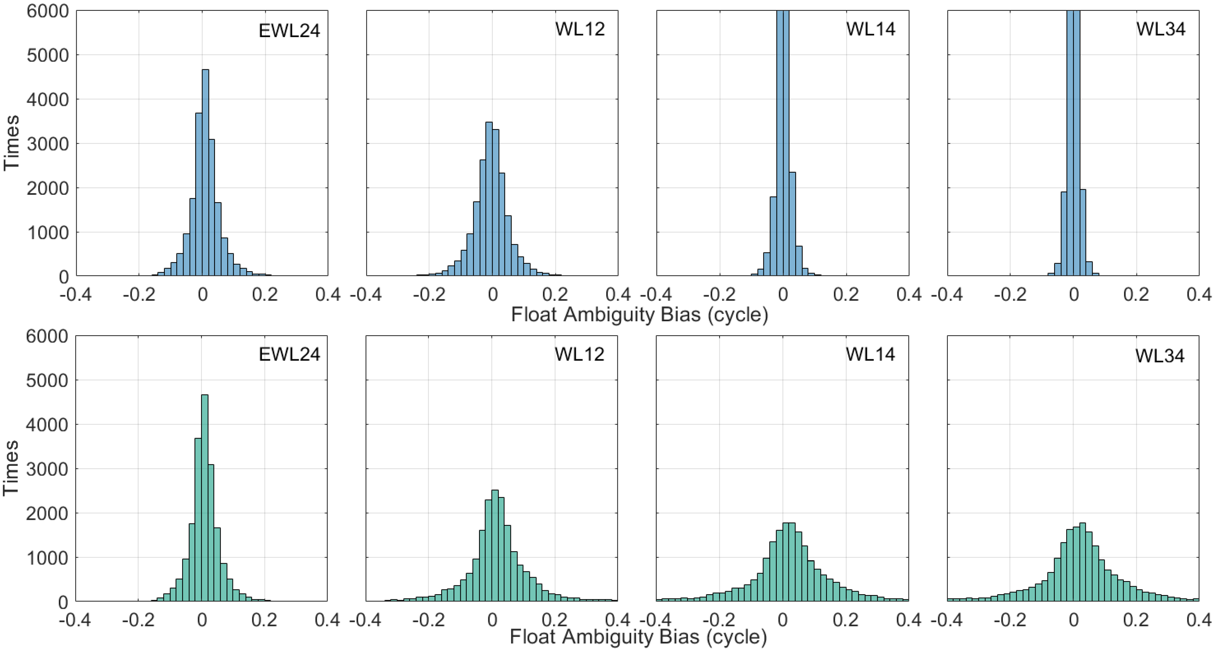
The floating solution biases of WL ambiguities were counted, and are displayed as histograms in Figure 5. The upper panel shows the result after ionospheric correction, and the lower panel shows the result without ionospheric correction. It can be seen from the figure that the WL floating solution bias after ionospheric correction was more concentrated around 0 cycle, and most deviations are less than 0.1 cycles, especially for combinations WL₁₄ and WL₃₄.

The WL floating solution bias was calculated at intervals of 0.1 cycles, as shown in

Table 3. Statistics of EWL/WL float ambiguity bias.

Observation Type		Ambiguity Bias Threshold
		<0.1	<0.2	<0.3	<0.4	<0.5
Without ionosphere correction	EWL24	94.5	99.6	99.9	100.0	100.0
	WL12	76.2	93.3	97.7	99.1	99.7
	WL14	64.8	86.1	94.1	97.2	98.6
	WL34	64.1	85.5	93.7	97.0	98.5
With ionosphere correction	EWL24	-	-	-	-	-
	WL12	91.8	99.3	99.9	100.0	100.0
	WL14	99.7	100.0	100.0	100.0	100.0
	WL34	99.9	100.0	100.0	100.0	100.0

. Without correcting the ionosphere, the probability of deviation less than 0.5 cycles was 99.7/98.6/98.5% for combinations WL₁₂/WL_14/WL₃₄, respectively, which is also regarded as the WL ambiguity fixed success rate by rounding. The fixing success rate after ionospheric correction could reach 100%. In practical applications, the threshold for rounding the WL ambiguity to a fixed value is 0.3–0.4 cycles. The fixing threshold will directly reduce the number of satellites participating in the fixing by 3–6%, which will affect the positioning accuracy of users.

In order to further improve the accuracy of the estimated ionospheric delay, three sets of uncorrelated WL observations (WL₁₂/WL₁₄/WL₃₄) were selected for calculation, and the optimal value was estimated by LSE. Figure 6 shows the ionospheric delay calculated by various EWL and WL observations. It can be seen that $I_{EW{L}_{24}}$ had the largest noise, and $I_{W{L}_{14}}$ and $I_{W{L}_{34}}$ had the smallest noise, which is consistent with the theoretical value of the noise amplification factor given in Table 2. Ultimately, the amplification factor of the noise of the ionospheric delay estimated by LSE was about 4.5, corresponding to the basic ambiguity deviation of about 0.1 cycles.

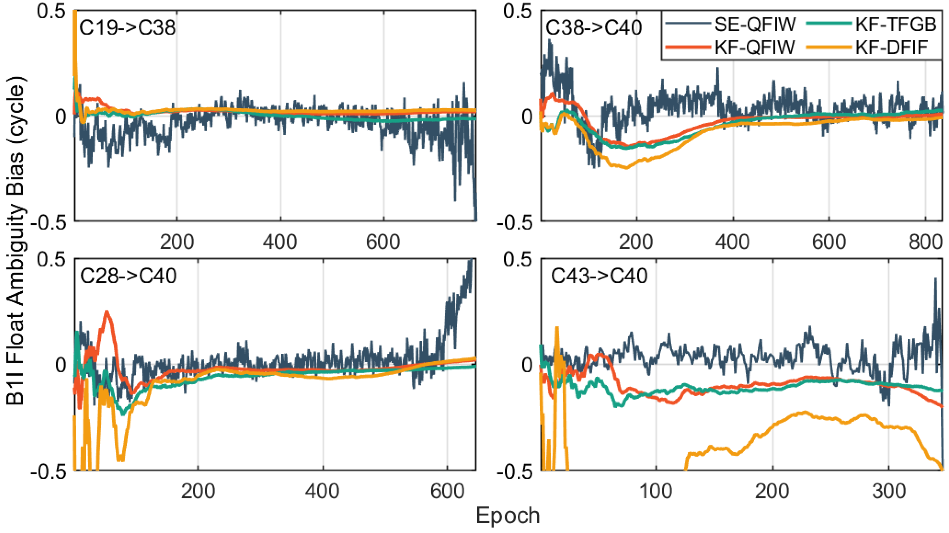
Figure 7 shows the deviations of basic float ambiguities calculated by the three models, DFIF, TFGB, and QFIW. The black, red, green, and orange lines indicate the float ambiguity bias calculated by the single epoch (SE) QFIW model, the KF-QFIW model, the KF-TFGB model, and the KF-DFIF model, respectively. It can be seen from the figure that the estimated bias calculated by the SE-QFIW model was mostly less than 0.5 cycles, which could be fixed correctly by rounding. Only at low elevation, some satellites’ ambiguity bias exceeded 0.5 cycles. The accuracy of the KF-QFIW model was further improved, especially for low-altitude satellites, and an almost 100% rounding fixing success rate could be achieved. The ambiguity bias of the TFGB model is pretty close to the QFIW model. For the DFIF model, due to the large, combined noise, the result was worse than the KF-QFIW model in both ambiguity accuracy and convergence speed.

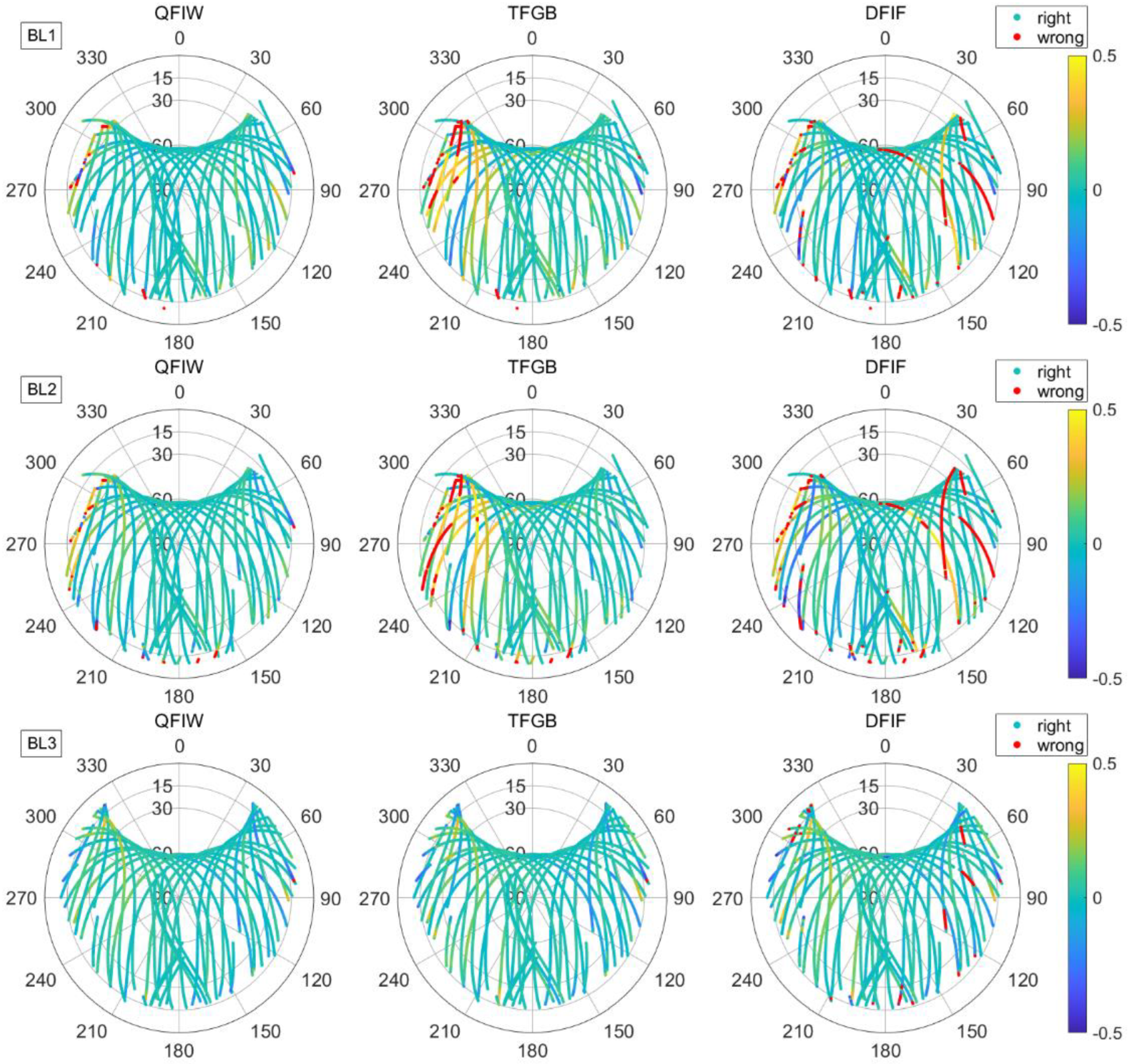
In order to compare the accuracy of the three processing models intuitively, we drew sky maps of the float ambiguity bias, as shown in Figure 8. From top to bottom in the figure are baselines BL1, BL2, and BL3. Red dots indicate deviation of more than 0.5 cycles, and other colors indicate deviation of less than 0.5 cycles. The corresponding relationship between bias and color is shown in the color bar on the right side of the figure. It can be seen from the figure that the floating ambiguity bias of the QFIW model was more than 0.5 cycles at individual low-altitude satellites only sporadically. However, there was a significantly larger proportion of float ambiguity bias of more than 0.5 cycles in the DFIF model, and some satellites exceeded the limit for a long time. The result of the TFGB model is between the two.

It can be seen from the statistical results in

Table 4. Statistics of basic ambiguity resolution success rate.

	BL1 (%)	BL2 (%)	BL3 (%)
QFIW	99.66	99.64	99.98
TFGB	98.32	97.81	99.98
DFIF	96.98	95.61	98.74

that utilizing the QFIW model proposed in this study and the rounding fixing strategy, the ambiguity resolution success rate of the three baselines was 99.66, 99.56, and 99.96%; compared with 96.96, 95.61, and 98.74% for the traditional DFIF model and 98.32, 97.81, and 99.98% for the TFGB model, there was a significant improvement. When the LAMBDA (least-square ambiguity decorrelation adjustment) search strategy was used, the QFIW model was still slightly improved compared to the traditional DFIF and TFGB models.

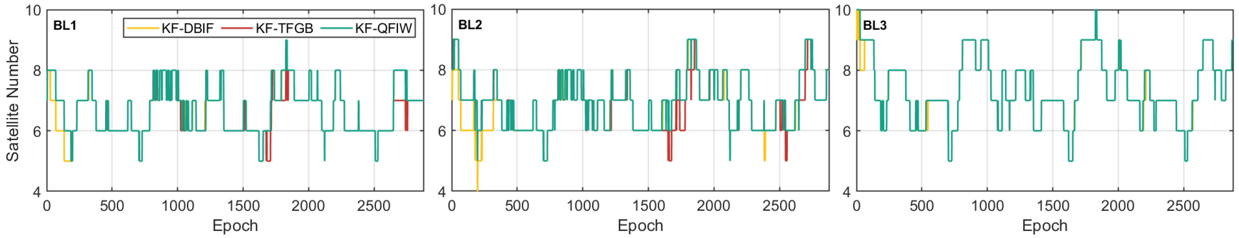
In addition, we made a comparative analysis of the two models on a time scale, and drew a time-sequence diagram of the number of satellites successfully fixed by the two models. It can be seen from Figure 9 that the QFIW model successfully fixed more satellites than the DFIF and TFGB models. In the initialization phase, the advantages of the QFIW model were more obvious. Within 300 s after initialization, the number of satellites it successfully fixed was 7.7, 13.3, and 2.1% higher for the three baselines compared to the DFIF model.

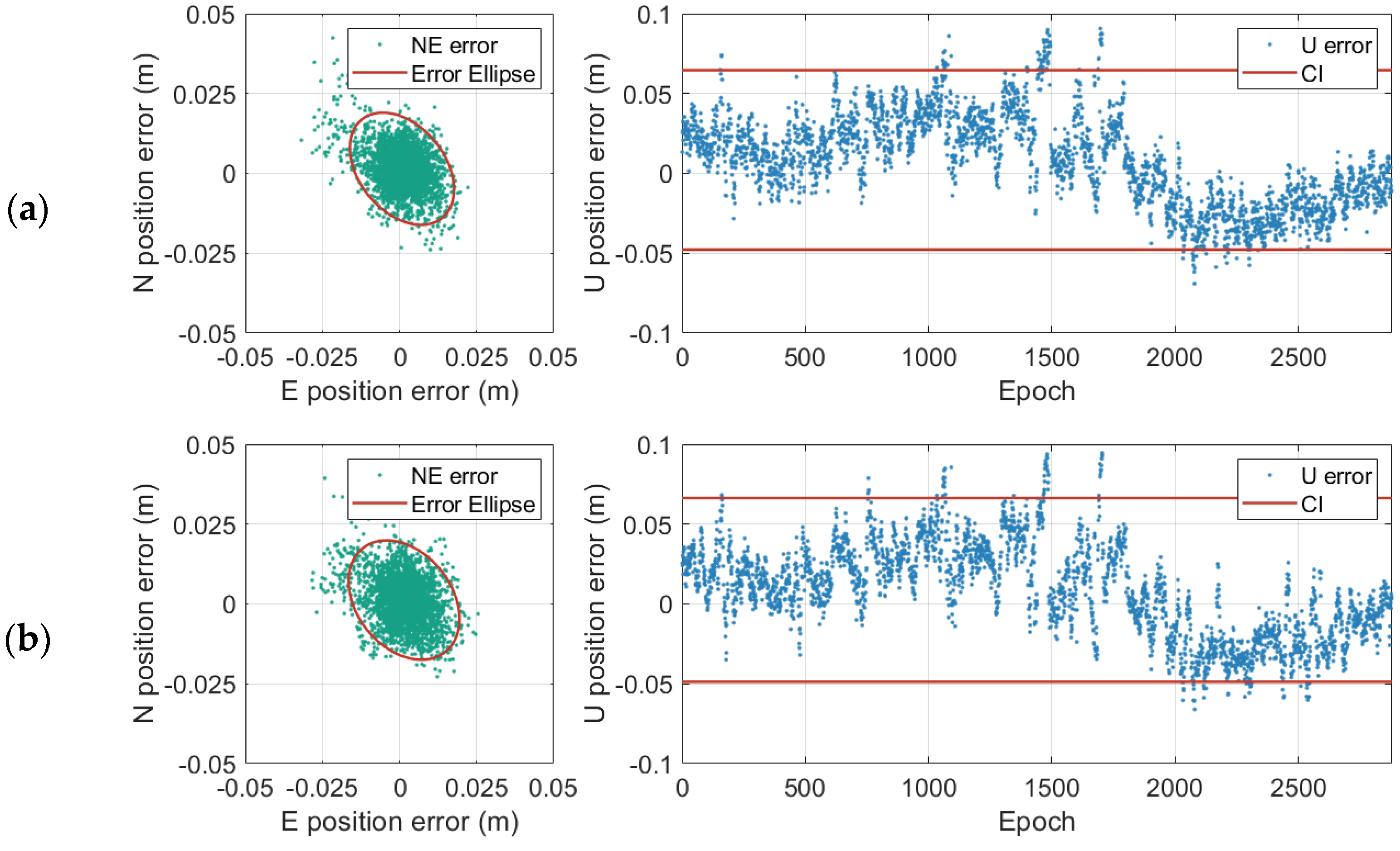
Interpolating ionospheric and tropospheric delays at the user’s position is the key to realizing the user’s high-precision positioning. Based on basic ambiguity fixing, the ionospheric and tropospheric delays at each baseline could be calculated, and the atmospheric error at the user’s position could be interpolated by LIM/LSM/DIM or other models. In this study, the LSM model was selected for atmospheric interpolation [26], and the user positioning results are shown in Figure 10. The green and blue dots in the figure comprise a scatter diagram of positioning error, and the red line represents the error ellipse or 95% confidence interval (CI). The root mean square (RMS) values of the positioning results were 0.0069/0.0072/0.0281 m for E/N/U directions, respectively, for the QFIW model, 0.0073/0.0076/0.0288 m for the TFGB model, and 0.0085/0.0103/0.0342 m for the DFIF model. It can be concluded that using the QFIW model to fix the ambiguity between reference stations could significantly improve the user’s positioning accuracy.

For the second CORS network, the base stations and user station also had the same types of receiver and antenna—the CHCNAV P5 receiver (with UNICORE UB4B0 board) and the CHCNAV AT611 antenna. The average length of the three baselines was about 50 km. Observations of DOY 169–175, 2021, were used for experimental verification in this study. The elevation mask was set to 10°, and the sample rate was 10 s. Figure 11 displays the geographical location of the stations. The data processing strategy was consistent with the first CORS.

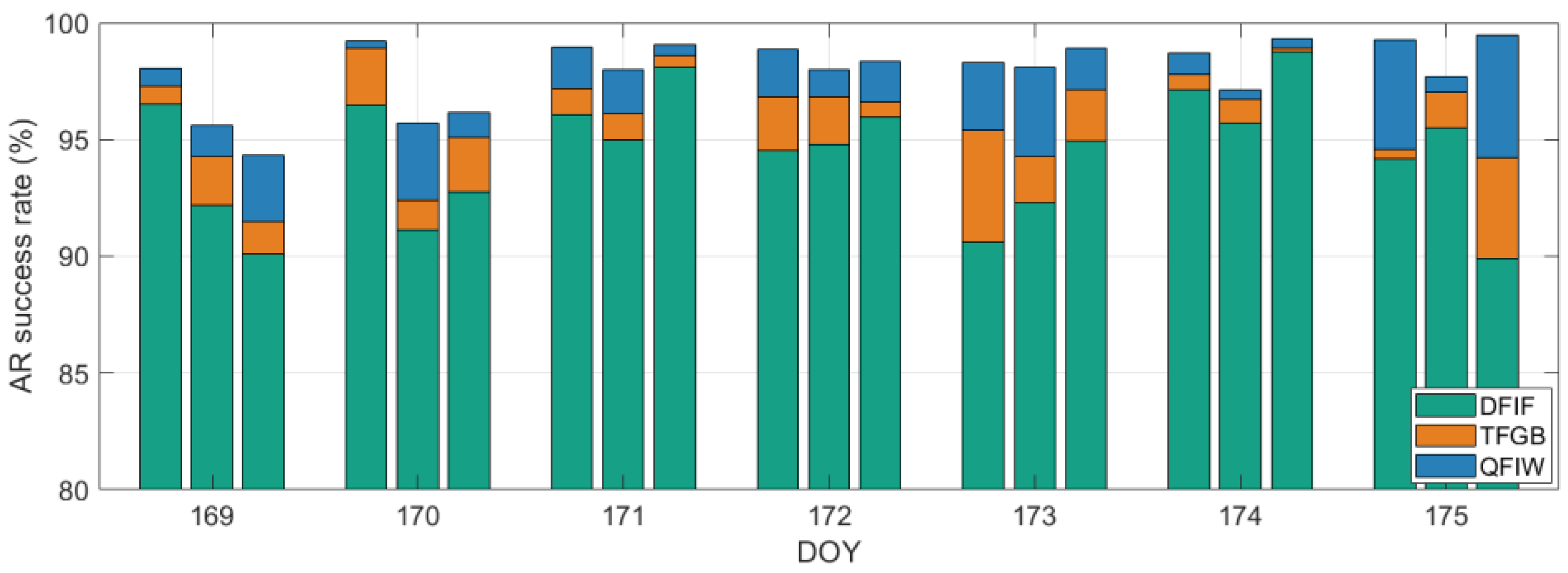
Figure 12 shows the ambiguity fixing success rate of three baselines for seven consecutive days under the two models. The three bars, from left to right, for each day represent baseline JN-JR, JN-LI, and JR-LI, respectively. It can be seen from the figure that the QFIW model had a better success rate than the TFGB and DFIF models for all baselines on all days. The success rate increased from 94.4 and 96.1% to 98.0% compared with the DFIF and TFGB models.

Figure 13 illustrates the user positioning errors under the three models. The three bars, from left to right, for each day represent E, N, and U directions. It can be seen from the figure that the positioning errors were better for the QFIW model than the DFIF and TFGB models on all seven days. For the QFIW model, the plane positioning error was always better than 2 cm, while the maximum vertical error exceeded 6 cm, which may have been caused by large atmospheric modeling error and multipath delay.

We calculated the statistics of the positioning results of the three models, and the results are shown in

Table 5. Positioning error statistics of three models.

	QFIW			TFGB			DFIF
	E (m)	N (m)	U (m)	E (m)	N (m)	U (m)	E (m)	N (m)	U (m)
DOY169	0.0128	0.0108	0.0341	0.0143	0.0113	0.038	0.0177	0.012	0.0422
DOY170	0.0135	0.0119	0.048	0.0146	0.0158	0.0513	0.0173	0.0178	0.0605
DOY171	0.016	0.0113	0.0518	0.016	0.0128	0.0531	0.0164	0.0142	0.055
DOY172	0.0123	0.0107	0.061	0.0138	0.0221	0.0652	0.0215	0.027	0.0738
DOY173	0.01	0.0102	0.0626	0.011	0.0112	0.063	0.011	0.0135	0.0675
DOY174	0.0096	0.0089	0.0575	0.0098	0.0101	0.0616	0.0106	0.0108	0.0631
DOY175	0.0104	0.0111	0.0407	0.0108	0.0138	0.0453	0.0121	0.0141	0.0472
Average	0.0121	0.0107	0.0508	0.0129	0.0139	0.0539	0.0152	0.0156	0.0585

. As summarized in Table 5, the average positioning error was 0.0121/0.0107/0.0508 m for E/N/U directions, respectively, for the QFIW model, and 0.0152/0.0156/0.0585 m for the DFIF model, with the positioning accuracy in the three directions improved by 20.6/31.5/13.1%; the average positioning error was 0.0129/0.0139 and 0.0539 m for the TFGB model, with the positioning accuracy improved by 6.3/22.9/5.8%.

4. Discussion

First, we studied the advantages of BDS-3 quad-frequency observations in the ambiguity resolution of WL. Using step-by-step fixing and ionospheric delay correction with EWL/WL, the accuracy of the WL floating ambiguity was greatly improved. We could achieve a 100% fixing success rate with an epoch, which is significantly higher than the traditional dual-frequency algorithm, as shown in Figure 5. Then, using the LSE and ionospheric delay calculated by three sets of independent WL ambiguities, the ionospheric delay of the basic frequency and its variance were calculated. The estimated ionospheric delay noise of basic frequency was about 0.1 week, which had little effect on the basic ambiguity fixing.

After that, the ionospheric delay constraint equation was added to construct the QFIW model. Compared with the DFIF and TFGB models, the basic ambiguity floating-point solution estimated by the QFIW model was more accurate, and in most cases the floating ambiguity deviation was less than 0.5 weeks. For satellites above 30°, the QFIW model could achieve a 100% fixing success rate; for low-altitude satellites, the fixing success rate was also greatly improved, as shown in Figure 8. Figure 13 shows the results of user positioning accuracy using virtual observations generated by the three methods. Since the wrong fixed satellites were not eliminated, outliers appeared in some epochs, so the positioning error in the U direction was relatively large. However, the advantages of the QFIW model compared to the DFIF and TFGB models can still be intuited from the figure.

For some low-altitude satellites, the QFIW model still had ambiguity resolution errors, which may have been caused by tropospheric residual delay and large multipath delay. In the follow-up, it will be necessary to continue to study the advantages of multi-frequency observations in reducing the tropospheric delay and improving the fixing success rate of the DFIW model at low altitude.

5. Conclusions

Based on BDS-3 quad-frequency observation data, addressing the large noise of the traditional dual-frequency ionosphere-free model (DFIF), a quad-frequency ionosphere-weighted (QFIW) model was proposed to realize fast and accurate fixing of the basic ambiguity between reference stations. For the traditional DFIF and TFGB models, it has been demonstrated that the wide-lane (WL) ambiguity will be fixed at wrong integers after smoothing due to the influence of residual tropospheric and multipath delays. Moreover, due to the large noise of ionosphere-free (IF) combinations, the estimated floating-point ambiguities are inaccurate. The QFIW model proposed in this study could effectively improve the rounding success rate of WL and basic ambiguities.

First, based on the combined observation theory, considering the wavelength and noise amplification factor of the combinations, an EWL observation (0, 1, 0, −1) and three independent WL observations (1, −1, 0, 0), (1, 0, 0, −1), and (0, 0, 1, −1) were selected. Then, on the basis of fixing the ambiguities of the EWL by smoothing and rounding, the ambiguities of the three WL combinations were fixed one-by-one with ionospheric delay correction; the double-differenced ionospheric delays $I_{W{L}_{12}}$, $I_{W{L}_{14}}$, and $I_{W{L}_{34}}$ were calculated by the fixed-ambiguity WL observations. Finally, the ionospheric correction values of the basic frequency point were estimated by LSE with three independent ionospheric delays. In addition, taking the estimated ionospheric correction values as a priori information, the ionosphere-weighted model was constructed with uncombined code and phase observations. The basic ambiguities were fixed by KF and rounding. Finally, based on the fixed basic ambiguities between reference stations, virtual observation values were generated, and user positioning accuracy was evaluated.

In this study, real data of two CORS (DOY 148 in 2020 and 169–195 in 2021) were used to verify the proposed algorithm. The rounding success rate of the WL ambiguity was significantly improved with ionospheric correction. Even when the rounding threshold was set to 0.3 cycles, an almost 100% success rate could be achieved. Then, we analyzed the advantages of the QFIW model from the two scales of space and time and found that the model significantly improved the accuracy of the basic ambiguity estimations for high-altitude-angle satellites and at the initial stage of initialization, and had good performance for low-altitude-angle satellites. According to the statistical results, the QFIW had a better success rate than the DFIF and TFGB models for all baselines on all days, and the success rate increased from 94.4 and 96.1% to 98.0%. Furthermore, the user positioning accuracy was improved by 20.6, 31.5, and 13.1% for E, N, and U directions compared with the DFIF model, and by 6.3, 22.9, and 5.8% compared with the TFGB model.

References

1. Zhang, X.; Li, X.; Lu, C.; Wu, M.; Pan, L. A comprehensive analysis of satellite-induced code bias for BDS-3 satellites and signals. Adv. Space Res. 2017, 63, 2822–2835. [Google Scholar] [CrossRef]
2. Fan, L.; Li, M.; Wang, C.; Shi, C. BeiDou satellite’s differential code biases estimation based on uncombined precise point positioning with triple-frequency observable. Adv. Space Res. 2017, 59, 804–814. [Google Scholar] [CrossRef]
3. Forssell, B.; Martin-Neira, M.; Harrisz, R.A. Carrier phase ambiguity resolution in GNSS-2. In Proceedings of the 10th International Technical Meeting of the Satellite Division of the Institute of Navigation (ION GPS 1997), Kansas City, MO, USA, 16–19 September 1997; pp. 1727–1736. [Google Scholar]
4. Vollath, U.; Birnbach, S.; Landau, H.; Fraile-Ordonez, J.M.; Martin-Neira, M. Analysis of three-carrier ambiguity resolution technique for precise relative positioning in GNSS-2. J. Inst. Navig. 1999, 46, 13–24. [Google Scholar] [CrossRef]
5. Jung, J.; Enge, P.; Pervan, B. Optimization of cascade integer resolution with three civil GPS frequencies. In Proceedings of the 13th International Technical Meeting of the Satellite Division of The Institute of Navigation (ION GPS 2000), Salt Lake City, UT, USA, 19–22 September 2000; pp. 2191–2200. [Google Scholar]
6. Hatch, R.; Jung, J.; Enge, P.; Pervan, B. Civilian GPS: The benefits of three frequencies. GPS Solut. 2000, 3, 1–9. [Google Scholar] [CrossRef]
7. Richert, T.; El-Sheimy, N. Optimal linear combinations of triple frequency carrier phase data from future global navigation satellite systems. GPS Solut. 2007, 11, 11–19. [Google Scholar] [CrossRef]
8. Feng, Y.; Li, B. A benefit of multiple carrier GNSS signals: Regional scale network-based RTK with doubled inter-station distances. J. Spat. Sci. 2008, 53, 135–147. [Google Scholar] [CrossRef] [Green Version]
9. Li, B. Review of triple-frequency GNSS: Ambiguity resolution, benefits and challenges. J. Glob. Position. Syst. 2018, 16, 1–11. [Google Scholar] [CrossRef]
10. Ericson, S. A study of linear phase combinations in considering future civil GPS frequencies. In Proceedings of the 1999 National Technical Meeting of The Institute of Navigation, San Diego, CA, USA, 25–27 January 1999; pp. 677–686. [Google Scholar]
11. Feng, Y.; Rizos, C. Geometry-based TCAR models and performance analysis. In Observing our Changing Earth; Springer: Berlin/Heidelberg, Germany, 2009; pp. 645–653. [Google Scholar]
12. Feng, Y.; Rizos, C. Three carrier approaches for future global, regional and local GNSS positioning services: Concepts and performance perspectives. In Proceedings of the 18th International Technical Meeting of the Satellite Division of the Institute of Navigation (ION GNSS 2005), Long Beach, CA, USA, 13–16 September 2005; pp. 2277–2287. [Google Scholar]
13. Li, B.; Feng, Y.; Shen, Y. Three carrier ambiguity resolution: Distance-independent performance demonstrated using semi-generated triple frequency GPS signals. GPS Solut. 2010, 14, 177–184. [Google Scholar] [CrossRef]
14. Gao, W.; Gao, C.; Pan, S.; Wang, D.; Wang, S. Single-epoch positioning method in network RTK with BDS triple-frequency widelane combinations. Acta Geod. Cartogr. Sin. 2015, 44, 641–648. [Google Scholar]
15. Wang, K.; Rothacher, M. Ambiguity resolution for triple-frequency geometry-free and ionosphere-free combination tested with real data. J. Geod. 2013, 87, 539–553. [Google Scholar] [CrossRef] [Green Version]
16. Liu, G.; Zhang, X.; Li, P. Improving the performance of Galileo uncombined precise point positioning ambiguity resolution using triple-frequency observations. Remote Sens. 2019, 11, 341. [Google Scholar] [CrossRef] [Green Version]
17. Li, P.; Jiang, X.; Zhang, X.; Ge, M.; Schuh, H. GPS+ Galileo+ BeiDou precise point positioning with triple-frequency ambiguity resolution. GPS Solut. 2020, 24, 1–13. [Google Scholar] [CrossRef]
18. Geng, J.; Guo, J.; Meng, X.; Gao, K. Speeding up PPP ambiguity resolution using triple-frequency GPS/BeiDou/Galileo/QZSS data. J. Geod. 2020, 94, 1–15. [Google Scholar] [CrossRef] [Green Version]
19. Weber, R.; Karabatic, A. Potential improvements in GNSS-based troposphere monitoring by use of upcoming GALILEO signals. In Proceedings of the 2nd Colloquium-Scientifc and Fundamental Aspects of the Galileo Program, Padua, Italy, 14–16 October 2009. [Google Scholar]
20. Wang, K.; Khodabandeh, A.; Teunissen PJ, G. Five-frequency Galileo long-baseline ambiguity resolution with multipath mitigation. Gps Solut. 2018, 22, 1–14. [Google Scholar] [CrossRef] [Green Version]
21. Li, B.; Zhang, Z.; Miao, W.; Chen, G.E. Improved precise positioning with BDS-3 quad-frequency signals. Satell. Navig. 2020, 1, 1–10. [Google Scholar] [CrossRef]
22. Jin, S.; Su, K. PPP models and performances from single- to quad-frequency BDS observations. Satell. Navig. 2020, 1, 13. [Google Scholar] [CrossRef]
23. Ge, Y.; Ding, S.; Qin, W.J.; Zhou, F.; Yang, X.H.; Wang, S.L. Performance of ionospheric-free PPP time transfer models with BDS-3 quad-frequency observations. Measurement 2020, 160, 107836. [Google Scholar] [CrossRef]
24. Teunissen, P. The geometry-free GPS ambiguity search space with a weighted ionosphere. J. Geod. 1997, 71, 370–383. [Google Scholar] [CrossRef] [Green Version]
25. Li, B.; Feng, Y.; Gao, W.; Li, Z.; Bofeng, L.; Yanming, F.; Weiguang, G.; Zhen, L. Real-time kinematic positioning over long baselines using triple-frequency BeiDou signals. IEEE Trans. Aerosp. Electron. Syst. 2016, 51, 3254–3269. [Google Scholar] [CrossRef]
26. Zhao, C.; Bei, J.; Dang, Y.; Liu, X. Analysis on Ionosphere Interpolation Models. J. Geomat. Sci. Technol. 2013, 30, 140–143, 148. [Google Scholar]
Figure 1. Algorithm process of the quad-frequency ionosphere-weighted model.
Remotesensing 14 01654 g001
Figure 2. AR (ambiguity resolution) success rates of DFIF (double-frequency ionosphere-free) and QFIW (quad-frequency ionosphere-weighted) models under different system errors and phase errors: (a,b).
Remotesensing 14 01654 g002
Figure 3. Distribution of first CORS (Continuously Operating Reference Stations) and user station.
Remotesensing 14 01654 g003
Figure 4. Float ambiguity bias of EWL (extra-wide-lane)/WL (wide-lane).
Remotesensing 14 01654 g004
Figure 5. Histograms of EWL/WL float ambiguity bias.
Remotesensing 14 01654 g005
Figure 6. Ionosphere delay calculated by EWL24/WL12/WL14/WL34 observations.
Remotesensing 14 01654 g006
Figure 7. The B1I float ambiguity bias calculated by the QFIW, TFGB (triple-frequency geometry-based) and DFIF model.
Remotesensing 14 01654 g007
Figure 8. Basic float ambiguity bias for three baselines calculated by QFIW, TFGB, and DFIF models.
Remotesensing 14 01654 g008
Figure 9. Number of satellites successfully fixed by QFIW, TFGB, and DFIF models.
Remotesensing 14 01654 g009
Figure 10. User positioning errors by three models: (a) QFIW; (b) TFGB; (c) DFIF. (N means north direction, E means east direction, NE means north and east directions, U means up direction, CI means confidence interval).
Remotesensing 14 01654 g010aRemotesensing 14 01654 g010b
Figure 11. Distribution of second CORS and user station.
Remotesensing 14 01654 g011
Figure 12. AR success rate of seven days under three models.
Remotesensing 14 01654 g012
Figure 13. User positioning error of seven days under three models.
Remotesensing 14 01654 g013