Technical Note

Spatial Negative Co-Location Pattern Directional Mining Algorithm with Join-Based Prevalence

1
College of Earth Sciences, Guilin University of Technology, Guilin 541004, China
2
Guangxi Key Laboratory of Spatial Information and Geomatics, Guilin University of Technology, No. 12 Jian’gan Road, Guilin 541004, China
3
College of Information and Computer, Taiyuan University of Technology, Taiyuan 030024, China
*
Author to whom correspondence should be addressed.
Remote Sens. 2022, 14(9), 2103; https://doi.org/10.3390/rs14092103
Submission received: 18 January 2022 / Revised: 7 April 2022 / Accepted: 25 April 2022 / Published: 27 April 2022
(This article belongs to the Special Issue Artificial Intelligence and Remote Sensing Datasets)

Abstract

:
It is usually difficult for prevalent negative co-location patterns to be mined and calculated. This paper proposes a join-based prevalent negative co-location mining algorithm, which can quickly and effectively mine all the prevalent negative co-location patterns in spatial data. Firstly, this paper verifies the monotonic nondecreasing property of the negative co-location participation index (PI) value as the size increases. Secondly, using this property, it is deduced that any prevalent negative co-location pattern with size n can be generated by connecting prevalent co-location with size 2 and with an n − 1 size candidate negative co-location pattern or an n − 1 size prevalent positive co-location pattern. Finally, the experiment results demonstrate that while other conditions are fixed, the proposed algorithm has an excellent efficiency level. The algorithm can eliminate the 90% useless negative co-location pattern maximumly and eliminate the useless 40% negative co-location pattern averagely.

1. Introduction

After Yoo et al. proposed two co-location algorithms based on join and join-less methods [1,2,3,4,5], the method for co-location mining received increasing attention. Subsequently, in order to mine co-location patterns quickly, Wang et al. proposed a new co-location mining algorithm, CPI-Tree [6,7]. In recent years, many scholars were inspired by the transaction-based approach [8,9,10,11,12] and the transaction-free approach [13,14,15,16,17]. An increasing number of co-location pattern algorithms were also developed, including “fuzzy co-location pattern mining”, “parallel co-location pattern mining”, “the adaptive maximal co-location (AMCM) algorithm”, “efficient co-location pattern mining” and “co-location pattern mining with rare features” [18,19,20,21,22,23,24,25,26]. With the popularity of the join-less co-location mining algorithms, Zhou et al. applied co-location patterns to decision trees and proposed a co-location-based decision tree (CL-DT, a method of decision tree) [27] and the CL-DT method of maximum variance expansion [28]. Subsequently, to further study the join-less co-location algorithm, the maximal instance algorithm for the fast mining of spatial co-location patterns [29] and a book about data mining for co-location patterns [30] proposed by Zhou et al. have made great contributions to spatial mining [31,32,33,34,35,36]. To mine negative relationships in the dataset, Zheng et al. proposed some constraint conditions and mining algorithms for negative sequence PT [37]. Cao et al. proposed the E-NSP algorithm, which can effectively identify negative sequence PT [38,39,40,41,42,43], and Dong et al. proposed the F-NSP algorithm [44,45,46,47,48]. Although there are an increasing number of algorithms for spatial data mining at present, there are still some potentially useful patterns that are not fully developed, including the negative co-location pattern. In the study of negative co-location rules, many scholars proposed mining algorithms for association rules.
  • Related Work
In 2004, in order to more effectively mine the co-location patterns in spatial data, Huang et al. [4] first proposed a join-based algorithm on the basis of the Apriori algorithm. This algorithm can efficiently handle continuous spatial data and keep track of spatial information that is not modeled by transactions. However, this algorithm did not extend to mine nonlinear distribution spatial data sets. In 2016, Zhou et al. [28] proposed an MVU(maximum variance unfolding)-based CL-DT algorithm, which extend co-location mining method to nonlinear distribution in spatial data sets. This algorithm overcomes the deficiency of the traditional CL-DT method, in which the Euclidean distance of instances that are nonlinear distributions in high-dimensional space cannot accurately reflect the co-location relationship between instances. To further shorten the calculation amount and time, in 2021, Zhou et al. [29] first defined maximal instances and proposed a maximal instance algorithm. This algorithm constructed the RI-tree to find maximal instances from a spatial data set and pruned it to prevalent co-location patterns. Although both algorithms can find co-location very efficiently, they do not extend to negative co-location.
A mutually exclusive relationship is extremely important in aspects such as investment and construction planning. In order to solve the problem that the traditional co-location cannot mine the mutually exclusive relationship, in 2004, Wu et al. [37] first proposed a new pattern of negative co-location and defined the prevalent negative co-location pattern in order to research the negative relationship patterns in space. They called all unexpected patterns except positive co-location negative co-location, which solved the basic concept of negative co-location. The practical application significance of negative co-location is explained by taking the example of the mutually exclusive relationship between coffee and tea in the shopping baskets of supermarket customers. However, their definition about negative co-location has not been detailly given, and it is not clearly defined and inefficient. So, a more precise definition is needed. In 2010, Jiang et al. [49] proposed the accurate concept of negative co-location patterns and the calculation method of the PI value of negative co-location in order to more accurately define the negative co-location pattern and speed up the mining speed. They also proposed a “mining algorithm for spatial positive and negative patterns”, which is called the traditional algorithm in this paper. This algorithm can effectively mine negative co-location patterns and calculate whether negative co-location is prevalent. However, the disadvantage of this algorithm is that it cannot distinguish useless negative co-location and eliminate it, and a large number of useless negative co-location patterns need to be calculated. In 2021, Wang et al. [50] proposed an upward inclusive negative co-location pattern algorithm and proposed the concept of minimal negative co-location in order to find the co-location pattern more effectively. Their algorithm uses the upward inclusiveness of negative co-location patterns to mine all negative co-location patterns by adding the features to minimal negative co-locations. However, this algorithm does not save much calculation time because it needs to search for the minimal negative co-location pattern first, and the calculation method of minimal negative co-location is complicated; therefore, upward inclusion cannot effectively and completely remove the useless co-location pattern.
Spatial data mining with a negative co-location pattern can be significant because it can find features with strong negative correlations and determine mutually exclusive relationships between spatial features, which can play a vital role in many applications. For example, Cao et al. [39] proposed that with negative mining being applied to the detection of gene sequences, the birth of disabled babies can be effectively avoided by mining the negative co-location relationship between certain diseases and specific gene sequences. It is also possible to prevent the occurrence of diseases in advance by mining gene sequences. Zheng et al. [38] proposed an Apriori-like negative mining algorithm to mine the data of supermarket shopping baskets. He defined negative correlation as (1) A B = ; (2) s u p p   A     m s   a n d   s u p p   B     m s ; (3) s u p p   A ¬ B   m s   o r   s u p p   ¬ A B     m s ,   o r   s u p p   ¬ A ¬ B     m s . However, the algorithm was not extended to the mining of spatial negative co-location. Moreover, because a large number of useless negative mining need to be calculated, the pruning of the algorithm needs to be further improved. The two negative mining examples above discover that it must calculate a large number of useless negative co-location patterns to obtain prevalent negative co-location patterns. For this reason, this paper proposes a join-based algorithm, which avoids calculating a large number of useless co-location patterns and effectively mines prevalent negative co-location patterns. This paper also provides a directional mining algorithm. Given a specified space feature set Y and size number, the prevalent candidate negative co-location pattern can be quickly determined.
In summary, the main innovations of this paper can be condensed as follows:
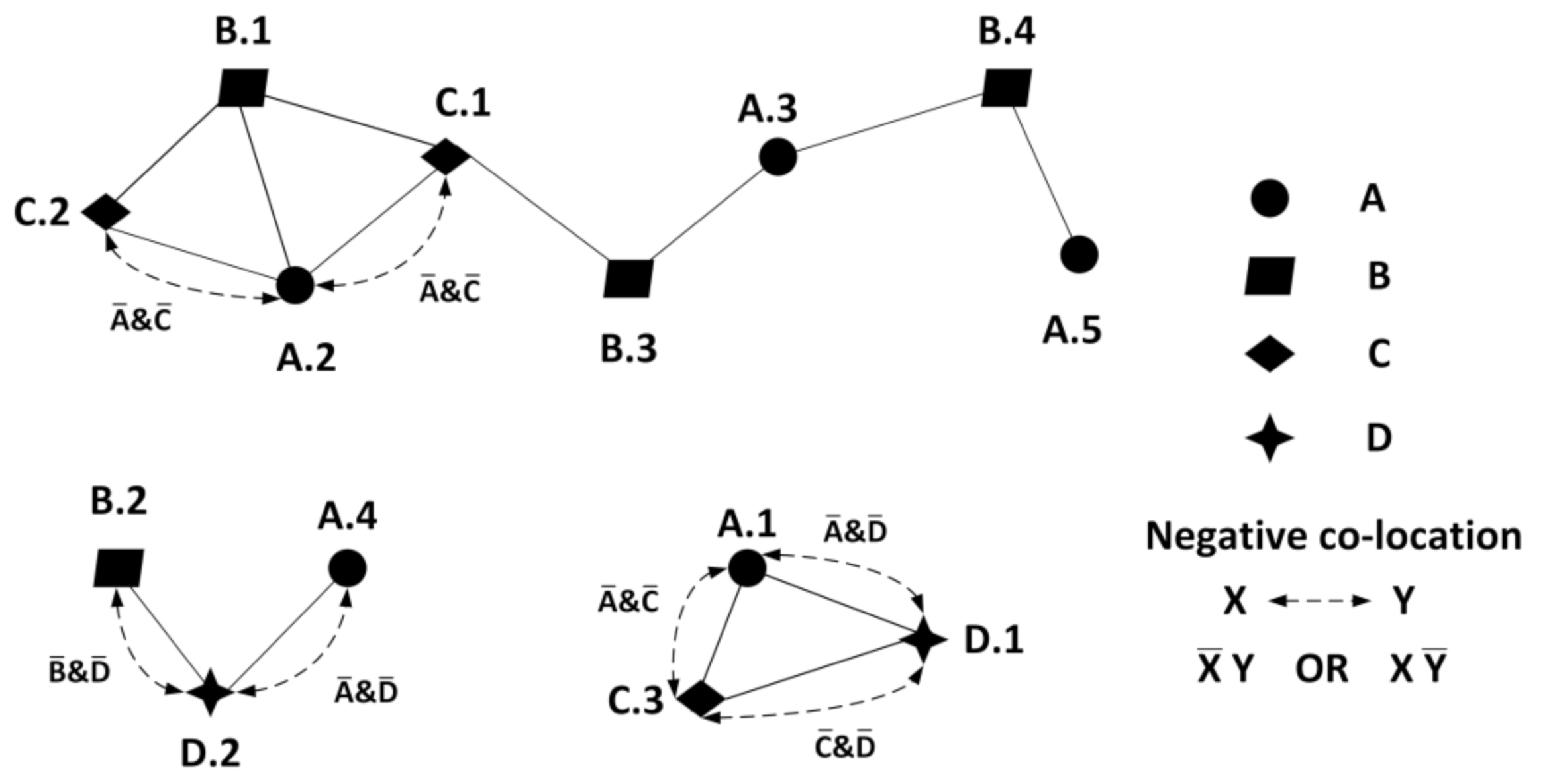
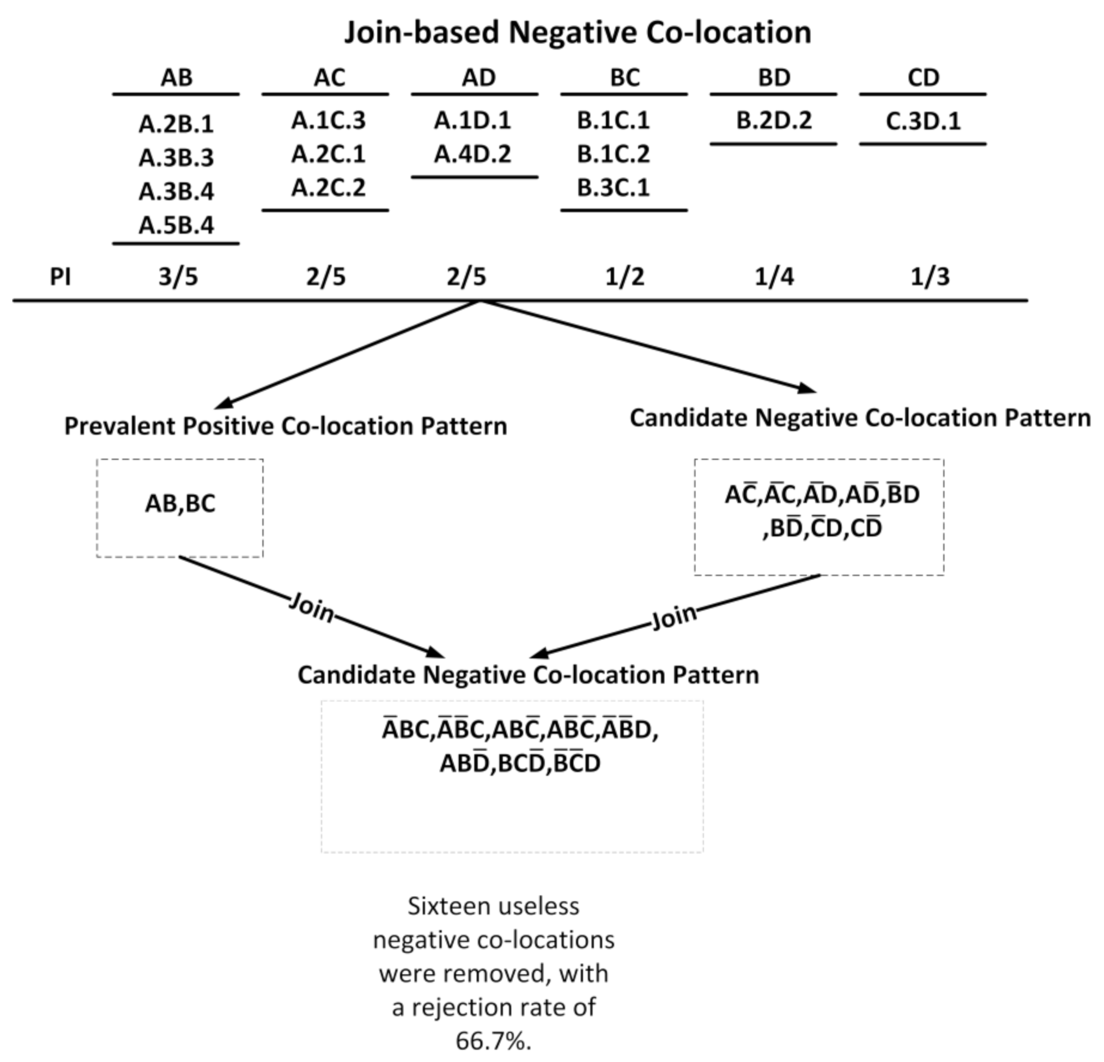
  • A candidate negative co-location pattern is proposed based on the definition [49] of prevalent negative co-location patterns. Additionally, we prove that any prevalent negative co-location pattern of size n can be generated by connecting the prevalent co-location of size 2 with an n − 1 size candidate negative co-location pattern or an n − 1 size prevalent positive co-location pattern.
  • For the specified spatial feature set Y , the negative co-location pattern T   =   X Y of the specified size can be calculated directly through the join-based algorithm.
  • According to the definition of a negative co-location pattern, the monotonous non-decrement of the PI value of a negative co-location pattern is strictly proven, and a quick pruning method is proposed by using this monotonous non-decrement of the PI value.
  • By combining the negative co-location patterns from small to large size, two patterns in extreme cases and their meanings are proposed: a “single positive of negative co-location pattern” and a “single negative of negative co-location pattern”. Additionally, an algorithm for solving the pattern is given.

2. Negative Co-Location Definition and Lemma

2.1. Preliminary Definitions

In this section, the abbreviations are explained as follows (Table 1):

2.2. Basic Definition of Negative Co-Location

Given a spatial feature set F = f 1 , f 2 , f 3 , , f n , the corresponding spatial feature instance set is S = s 1 , s 2 , s 3 , , s n . Given a relation R in a spatial feature instance, where R is assumed to be Euclidean distance and the threshold is d A .1 ,   B .1 S , R   A .1 , B .1 ( d i s t a n c e   A .1 , B .1   d , R can represent topological relationships (e.g., linked, intersection), distance relationships (e.g., Euclidean distance metric) and mixed relationships (e.g., the shortest distance between two points on a map) [49].
For a set of spatial instances, as shown in Figure 1, if two instances satisfy the relation R, they are connected by solid lines. If there is a candidate negative C-L relationship, it is connected with a dotted line.
Definition 1 (prevalent negative co-location pattern) [49].
“Given a minimum prevalent threshold (min_prev), a negative C-LP T   =   X Y is a prevalent negative C-LP if T meets the following conditions.”
“(1) P I X m i n _ p r e v ,   P I Y     m i n _ p r e v   a n d   P I X Y   <   m i n _ p r e
(2) P I T     m i n _ p r e v
Example 1.
In Figure 1, set the minimum threshold min_prev = 0.6, T   =   A B . The P I T   =   P I T ,   A   =   1     P R A ,   B ,   A   =   2 / 5 .   P I T   <   m i n _ p r e v , so T   =   A B is not prevalent.
Example 1 shows that it is impossible to directly calculate the participation rate PI of a negative C-LP at present. Only by calculating all the negative C-LP and corresponding PI of the C-LP can we judge whether it is a prevalent negative C-LP. However, the number of combinations of all negative C-LP is very large, and the amount of computation is very large. Most combinations are useless C-LP. The number of candidate negative C-LP that can be generated by an infrequent C-LP of size n is C n 1   +   C n 2   +   C n 3   +     +   C n n   =   2 n     1 . Therefore, the number grows exponentially. Once there are too many spatial features, the amount of calculation will be very large. To solve this problem, this paper proposes a join-based negative C-LP algorithm, which can quickly determine prevalent negative C-LP and greatly reduce the computation amount of useless negative C-LP.

2.3. Lemma and Definition of Join-Based Algorithm

Definition 2 (Single positive of negative co-location pattern).
If a negative C-LP T   =   F M and M = 1, this negative C-LP is called a single positive of negative C-LP.
If in a negative C-LP, there is only one negative spatial feature and the others are all positive, then M has a strong negative correlation with spatial feature objects such as F. For example, fungicides, herbicides and mosquito-repellent incense can kill or strongly repel a certain type of spatial characteristic object.
Definition 3 (Single negative of negative co-location pattern).
If a negative C-LP T   =   F M and F = 1, this negative C-LP is called a single positive of negative C-LP. The meaning is similar to the previous one.
Both of these PTs can be directly solved using the algorithm proposed in this paper, and the candidate negative C-LP with a specified spatial feature set and arbitrary size can be obtained.
Lemma 1.
For any negative C-LP T   =   F M , increase its spatial feature object; that is, with the increase in the size of the negative C-LP, the participation rate and participation degree are monotonically nondecreasing.
Proof. 
(1) The instance number of spatial features F i in negative C-LP F M is Number _ 1 i . The number of instances of spatial feature F i in negative C-LP F M is Number _ 2 i . T   =   F M ,   N   =   F M ,   F M . F and F in the same space features, in the F instance, will be in the F line of instance. However, due to the instance of rows that appear in F , they do not have to be in F. Thus, P R T ,   F i   =   F i     N u m b e r _ 1 i F i     F i     N u m b e r 2 i F i   =   P R N , F i ,   P I T   =   m i n F i     N u m b e r _ 1 i F i     m i n F i     N u m b e r _ 2 i F i   =   P I N .
(2) Assume T   =   F M ,   N   =   F M ,   M M   T   =   F M ,   N   =   F M .   Because   M M   MaxPR   T ,   F     MaxPR   N ,   F and PI T , F   =   1     MaxPR   T ,   F , P I N ,   F   =   1     M a x P R N ,   F .   T h e r e f o r e ,   P R N ,   F     P R T ,   F .
The equal sign holds if and only if M a x P R T , F   =   M a x P R N ,   F .
(3) Assume T   =   F M ,   N   =   F M ,   M M ,   F     F ,   T   =   F M ,   N   =   F M .   Because M     M ,   F F   MaxPR   T , F     MaxPR   N , F and PI T ,   F   =   1     MaxPR   T ,   F , PI N ,   F   =   1     MaxPR N , F   PR N ,   F     PR M ,   F .
The equal sign holds if and only if M a x P R T ,   F   =   M a x P R N ,   F .
Lemma 2.
For a prevalent negative C-LP T   =   F M , if F F and F is a prevalent C-LP, then T   =   F M is a prevalent negative C-LP.
Proof. 
For T   =   F M , because   T   =   F M is a prevalent negative C-LP ,   PI M min _ prev ,   PI F M     min _prev,   PI F M min _ prev . As the size of the C-LP increases, its PI is monotonically nonincreasing. Then, F   F ,   PI   F M min _ prev . Because   F is a prevalent C-LP ,   PI F min _ prev , namel PI M min _ prev ,   PI F min _ prev ,   PI M F min _ prev .   Because   PI F M min _ prev ,   F F , It can be obtained from Lemma 1   that   PI F M PI F M min _ prev . It is thus proved that T   =   F M is a prevalent negative C-LP. □
Lemma 3.
For a prevalent negative C-LP T   =   F M , if M M and M is a prevalent C-LP, then T   =   F M is a frequently negative C-LP.
Proof. 
T   =   F M is a prevalent negative C-LP. Therefore ,   PI F min _ pre ,   PI F M min _ prev ,   PI F M min _ prev . As the size of the C-LP increases, its PI is monotonically nonincreasing. In addition, M   M ;   therefore ,   PI F M min _ prev .   Because   M is a prevalent C-LP,   PI M min _ prev . Therefore,   PI M min _ prev , PI F min _ prev ,   PI F M min _ prev .   Because   PI F M min_prev ,   M   M . It can be obtained from Lemma 1 that   PI F M PI F M min _ prev . It is thus proved that T   =   F M is a prevalent negative C-LP. □
Definition 4 (Candidate negative co-location).
According to the definition of prevalent negative C-LP in Jiang et al. [49], to better calculate the prevalent negative C-LP, the negative C-LP that meets the following conditions is called the candidate negative C-LP: P I X m i n _ p r e v ,   P I Y m i n _ p r e v   a n d   P I X Y   <   m i n _ p r e v ”.
Lemma 4.
For any size n candidate negative C-LP, it must be composed of an SZ n − 1 candidate negative C-LP or prevalent C-LP connected to an SZ 2 prevalent C-LP.
Proof. 
Assume an SZ n candidate negative C-LP, T   =   F M . T h e r e f o r e   P I F min _ p r e v , P I M min _ prev .
  • (1) For any spatial feature in F   =   F 1 ,   F 2 ,   F 3 ,   ,   F n , if one of them is removed, P I F min _ p r e v will still be true. The C-LP composed of any two spatial features in F   =   F 1 ,   F 2 ,   F 3 ,   ,   F n must be the SZ 2 prevalent C-LP. In addition, if F   =   F 1 ,   F 2 ,   F 3 ,   ,   F n   1   M , P I F min _ p r e v , P I M min _ p r e v . If PI F M min _ prev , then it is prevalent C-LP. If PI F M < min _ prev , it is a candidate negative C-LP. T h e r e f o r e ,   P I F min _ p r e v , P I M min _ p r e v . If PI F M min _ prev , it is prevalent C-LP. If PI F M < min _ prev , it is a candidate negative C-LP.
  • (2) This is the same as M   =   M 1 ,   M 2 ,   M 3 ,   ,   M n . It is thus proved that any SZ n candidate negative C-LP must be composed of an SZ n − 1 candidate negative C-LP or prevalent C-LP connected to an SZ 2 prevalent C-LP. □
Lemma 5.
For any spatial feature set M, M   =   m , specify the prevalent negative C-LP of T   =   F M of SZ n. F must be an n m SZ prevalent C-LP in the space set and F M   =   .
Proof. 
B e c a u s e   T is a prevalent C-LP, F ,   M must be a prevalent C-LP. In addition, T is size n, so F is SZ n-m, and F M   =   .

2.4. An Illustrative Example of Join-Based Co-Location

For example, in Figure 1, given min_prev = 0.5, the steps to find all of its candidate negative C-LP are shown in Figure 2 and Figure 3.
After the candidate mode is determined, all prevalent C-LP can be quickly determined by the pruning method and PI value comparison.

3. Join-Based Negative Co-Location Algorithm

In this section, the J-B prevalent negative C-LP algorithm and J-B directional prevalent negative C-LP mining algorithm are proposed. The specific steps are as follows: Section 3.1. J-B Prevalent Negative C-LP Algorithm.

3.1. Join-Based Prevalent Negative Co-Location Pattern Algorithm

The join-based prevalent negative co-location pattern algorithm includes the following steps:
(1) Calculate the positive C-LP of all instances and use any algorithm for mining prevalent positive C-LP. Store all prevalent C-LP of SZ 2 and above and store PI values for all C-LP of size 2.
(2) Compare the PI value of the SZ 2 C-LP with the threshold value of min_prev. Find and store all the SZ 2 candidate negative C-LP. The prevalent negative C-LP of SZ 2 is calculated to facilitate pruning.
(3) Starting from SZ 2, an SZ 2 prevalent C-LP or candidate negative C-LP is connected to an SZ 2 prevalent C-LP to generate an SZ 3 candidate negative C-LP. Then, an SZ 3 prevalent C-LP or candidate negative C-LP is connected to an SZ 2 prevalent C-LP to generate an SZ 4 candidate negative C-LP, and so on.
(4) The candidate negative C-LP obtained is pruned. According to Lemmas 2 and 3, if the SZ 2 candidate negative C-LP connected is a prevalent negative C-LP, then it is a prevalent negative C-LP. The remaining unpruned candidate negative C-LP are judged by the comparison between the PI value and the set threshold value of min_prev to obtain prevalent negative C-LP.

3.2. Join-Based Prevalence Negative Co-Location Pattern Directional Mining Algorithm

This section introduces a J-B mining algorithm for directional prevalent negative C-LP. The algorithm proposed in this paper can quickly find the prevalent negative C-LP T = X Y   for the specified Y . Based on Lemma 5, once Y   and the size of the final prevalent negative C-LP T are determined, then the SZ of X is also determined. Then, the determined prevalent C-LP X and Y   are selected from the entire data set to be connected to become the candidate T. However, the traditional algorithm cannot give feedback to Y and can only calculate all the negative C-LP. We need to count 2 n − 1 negative C-LP to solve this. The specific steps are as follows:
(1) Calculate the C-L relationships for all instances. The prevalent positive C-LP is mined using any existing algorithm. Store all prevalent C-LP of SZ 2 and above.
(2) For the specified mining SZ k Y .
(3) According to Lemma 5, the negative C-LP of the specified SZ c Y must be formed by the prevalent C-LP of SZ (c − k) and the connection of Y .
(4) Loop through all the prevalent C-LP of SZ (c − k) and connect them with Y to generate a negative C-LP of SZ c.
(5) Finally, all candidate negative C-LP are obtained. These are compared with the threshold value to screen out the final SZ c prevalent negative C-LP Y .

4. Experiment and Analysis

To date, there are only a few studies on the mining of negative C-LP. To evaluate the filtering rate and effectiveness of the J-B prevalent negative C-LP algorithm proposed in this paper, Algorithms 1 and 2 proposed in this paper are compared with the algorithm in Jiang et al. [49] (referred to as the traditional algorithm) on real and synthetic datasets. All algorithms are written in Python, and the experimental environment is PyCharm running in Windows10.
Algorithm 1: Join-based prevalent negative co-location pattern algorithm.
1. Input
2.  F: Collection of spatial f 1 , f 2 , f 3 , , f n
3.  S: Set of spatial instances S 1 , S 2 , S 3 , , S m
4.  R: C-L relationship
5.  min_prev: Minimum PI threshold
6. Output:
7.  nPPC: SZ n prevalent positive C-L collection
8.  2CNC: SZ 2 candidate negative C-L collection
9.  2PNC: SZ 2 prevalent negative C-L collection
10.   nCNC: SZ n candidate negative C-L collection
11.   nPNC: SZ n prevalent negative C-L collection
12. Variable:
13.  NT: Instance C-L relation
14. Method:
15. Calculate all NT
16. Mine the set Nppc   =   n P P C 1 , n P P C 2 , n P P C 3 , , n P P C m
17. for each PT in 2 C N C & 2 P P C {
18.   PT & 2PPC → 3CNC
19.   if 3CNC is not repetitive
20.    put 3CNC in Set3CNC}
21. for each PT in 3 C N C & 3 P P C {
22.   PT & 2PPC → 4CNC
23.    if 4CNC is not repetitive
24.    put 4CNC in Set4CNC}
25. so on
26. for each PT in n 1 C N C & n 1 P P C {
27.   PT & 2PPC → nCNC
30.    if nCNC is not repetitive
31.    put nCNC in SetnCNC}
32. for each PT in nCNC{
33.  if PT ⊇ lowPNC
34.     PT is a nPNC}
35. for other PT in nCNC{
36.  if PI > min _ prev
37.     PT is a nPNC}
Algorithm 2: Join-based prevalent negative co-location pattern directional algorithm.
1. Input:
2.  F: Collection of spatial features   f 1 , f 2 , f 3 , , f n
3.  S: Set of spatial instances S 1 , S 2 , S 3 , , S m
4.  R: C-L relationship
5.  min_prev: Minimum PI threshold
6.  C: The SZ of the final directional mining
7.  K: The SZ of Y
8. Output:
9.   nPPC: SZ n prevalent positive C-L collection
10.  nCNC: SZ n candidate negative C-L collection
11.  nPNC: SZ n prevalent negative C-L collection
12. Variable:
13.  NT: Instance C-L relation
14. Method:
15. Calculate all NT
16. Mine the set Nppc = n P P C 1 , n P P C 2 , n P P C 3 , , n P P C m
17. for each PT in (c-k)PPC{
18.  for each X i ( c - k ) PPC {
19.     X i & Y → cCNC
20.    if cCNC is not repetitive
21.     put in SetcCNC
22.  }
23.}
24. for each PT in cCNC{
25.  if PI   min_prev
26.    PT is cPNC
27.    else delete}

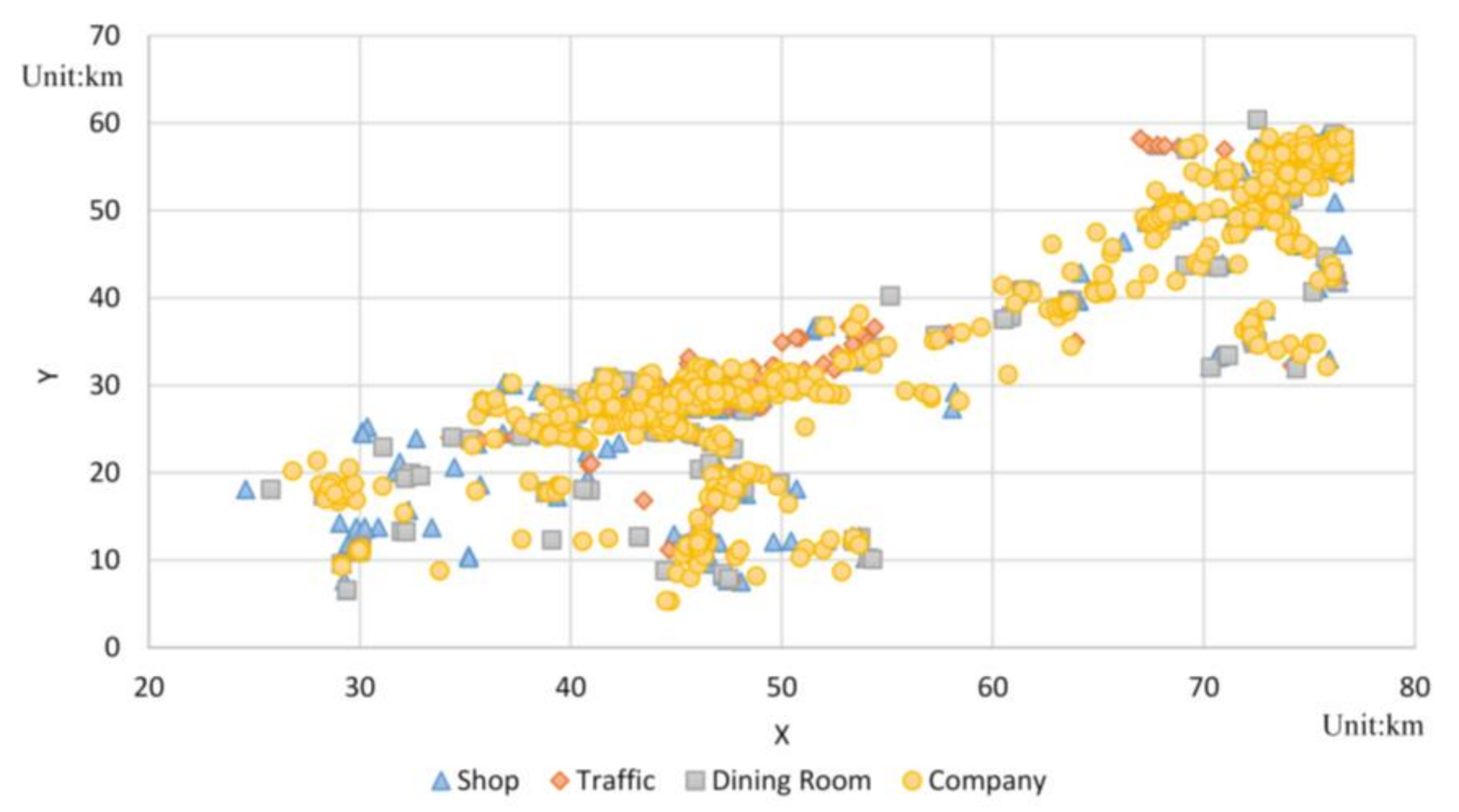
4.1. Experiment and Analysis of Real Data Sets

The real data set selected in the experiment is the distribution data from Shopping, Traffic, Dining and Companies in Jinan, Shandong, with a total of 11,189 data points. Among these four features, there is a negative C-L relationship between each of them. For example, most companies have their own staff canteens, and they are all free. Therefore, around the company, the number of other dining rooms may decrease. As another example, people do not choose to be next to their workplace most of the time when shopping, and they are more likely to choose entertainment complexes. In addition, most companies have commuter buses for their own employee routes, so other traffic may also be reduced. In this section of the experiment, different strong and weak negative C-LPs are mined by controlling the size of the min_prev value.
Convert the latitude and longitude of the data in Table 2 into the corresponding XY coordinate axes, as shown in Figure 4.
In the experiment in this section, the distance threshold was fixed at d = 1000 m. The participation threshold was changed from 0.1 to 0.7, and the relevant tests were performed.
According to the obtained data, a positive C-LSZ 1–4 was obtained, as shown in Figure 5. The line charts represent the sum of the total number of positive C-LP for each SZ, and the bar charts represent the number of detailed positive C-LP for each SZ.

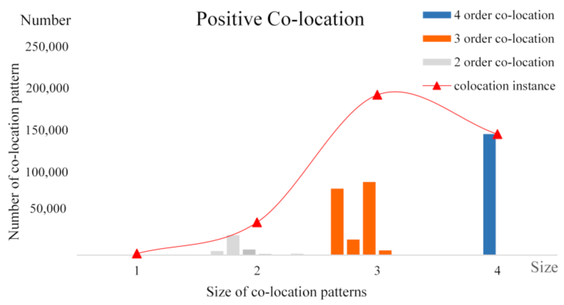
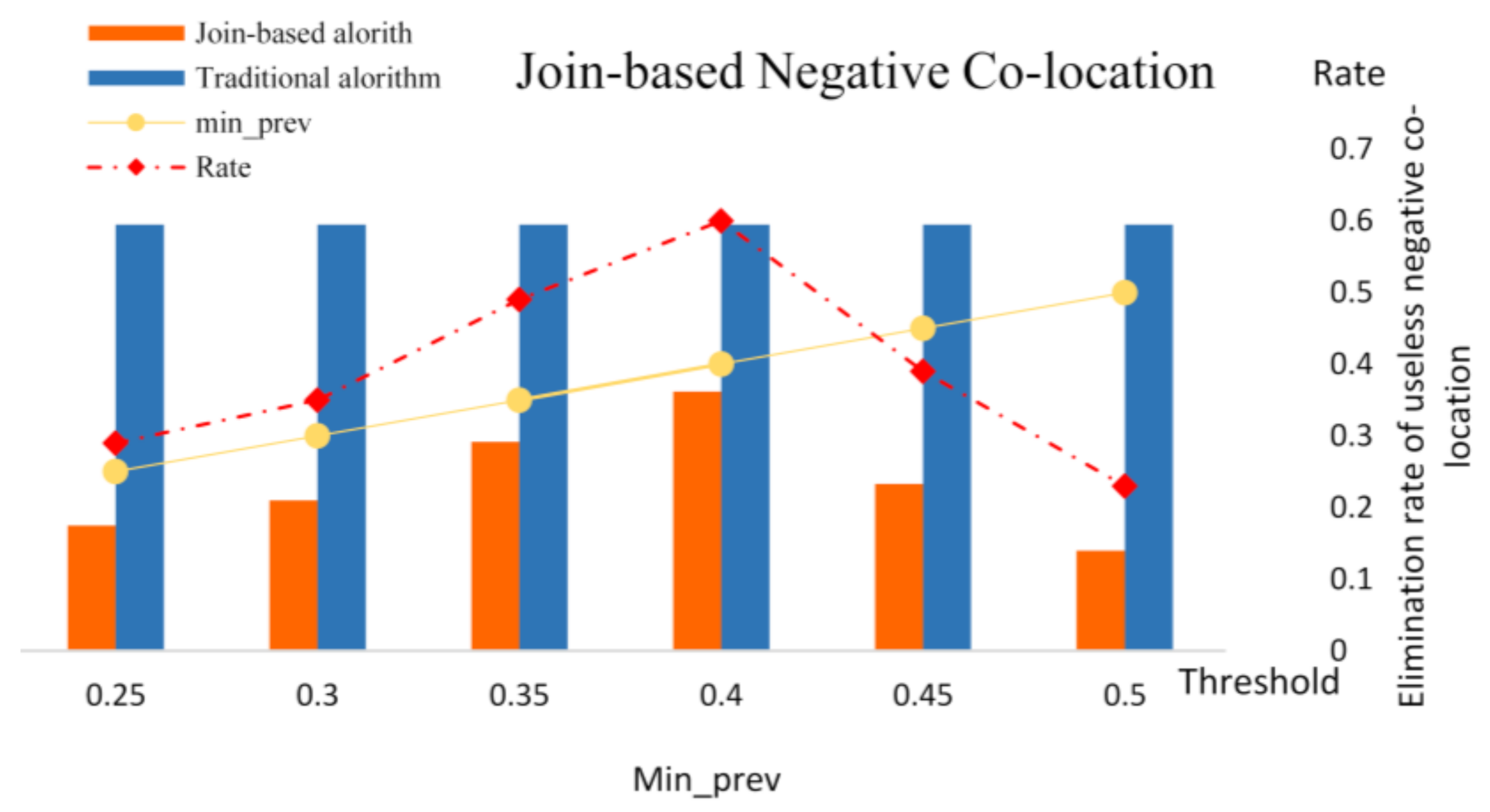
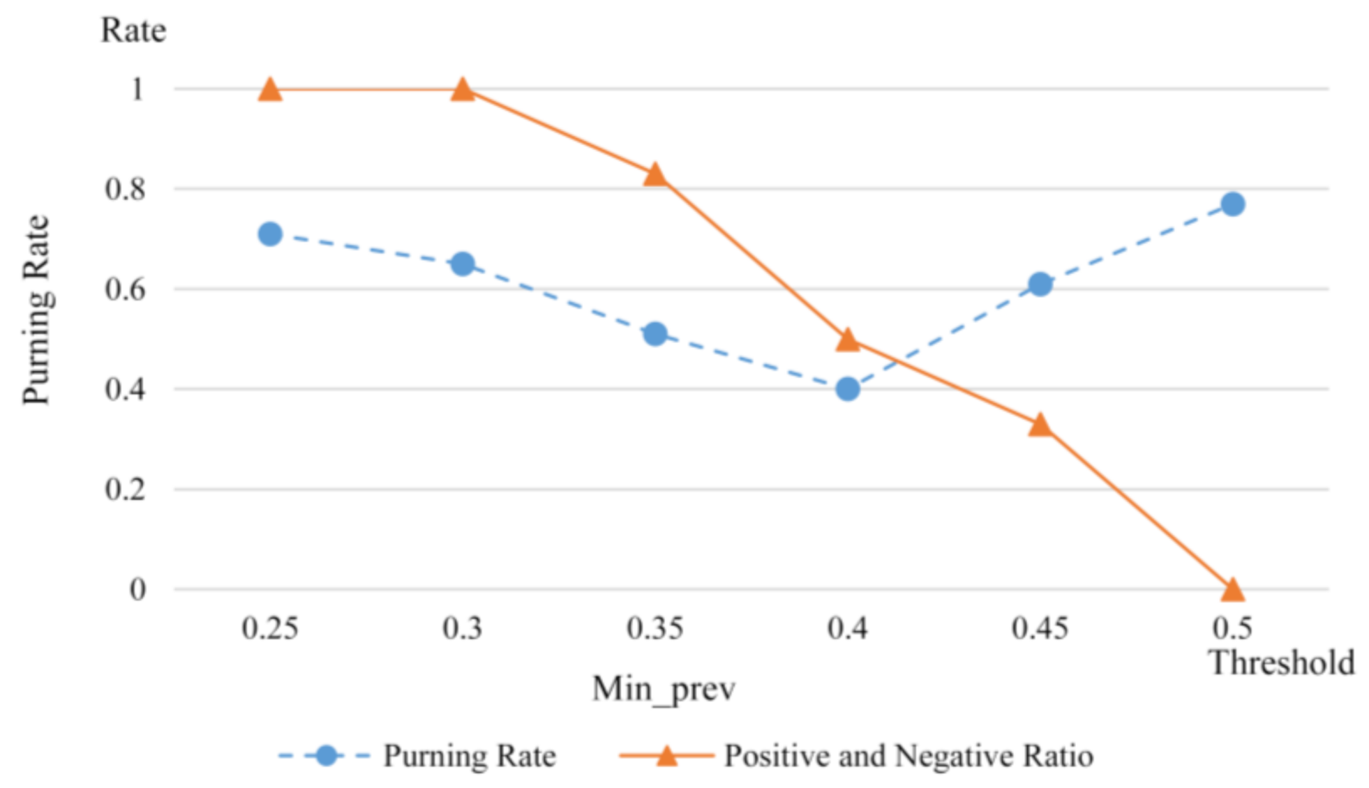
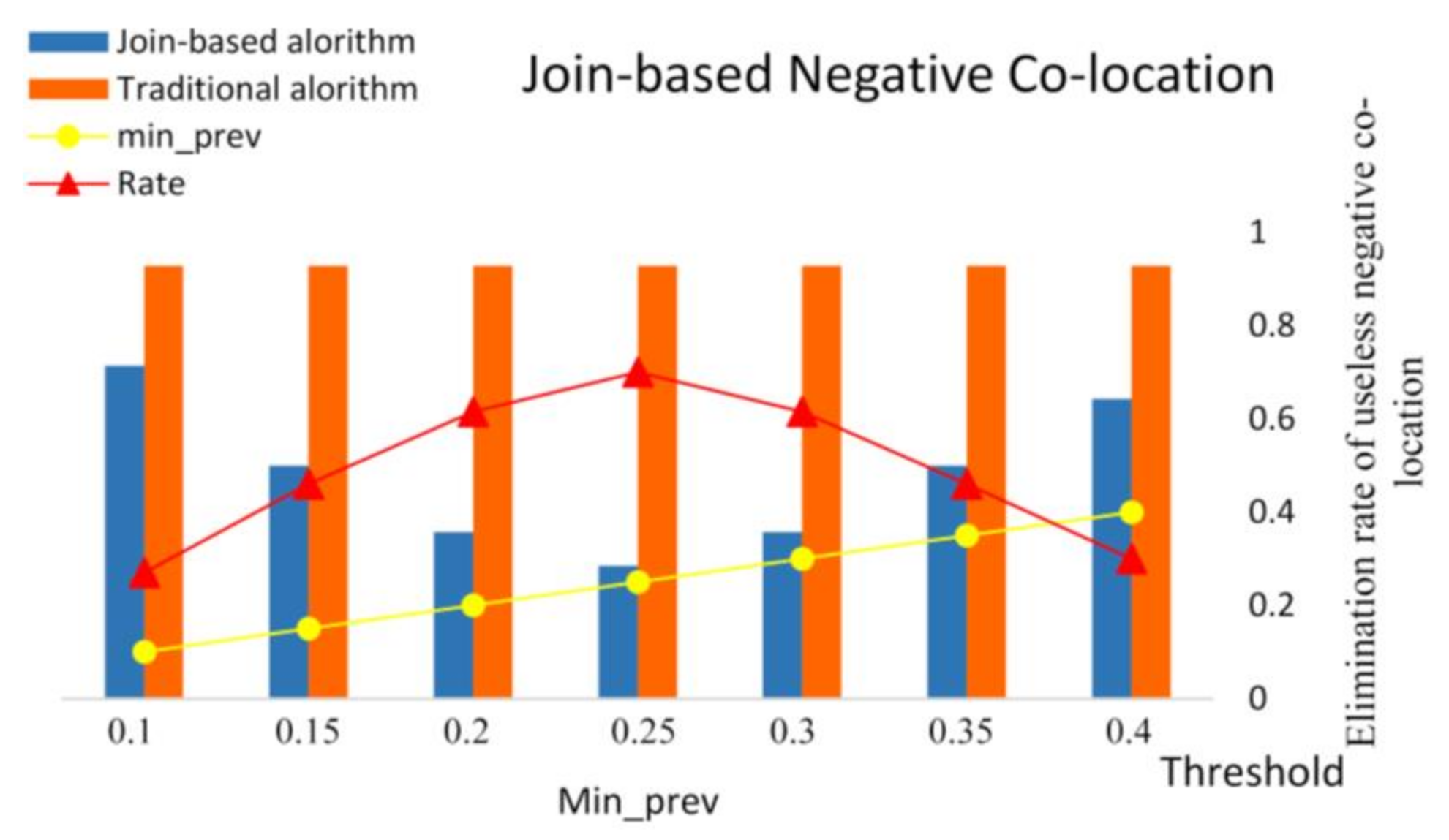
4.2. Experiment-1 with Join-Based Prevalent Negative Co-Location Pattern Algorithm

In this experiment, the traditional mining algorithm and J-B algorithm were used to mine all negative C-LP under different thresholds.
As seen in Figure 6 and Figure 7, the effect of the J-B algorithm changed with the change in min_prev. In this experiment, the prevalent negative C-LP under each threshold was certain. We observed that the two algorithms required a certain number of prevalent negative C-LP, the calculations that needed to be carried out, and the number of infrequent negative C-LP produced to determine the quality of the algorithm. When the number of prevalent C-LSZ 2 was equal to the number of candidate negative C-LSZ 2, it was the most complex, and the effect was the worst, but its number was approximately 0.6 of the traditional algorithm. The traditional algorithm enumerates all negative C-LP, independent of the value of min_prev, without fluctuations.

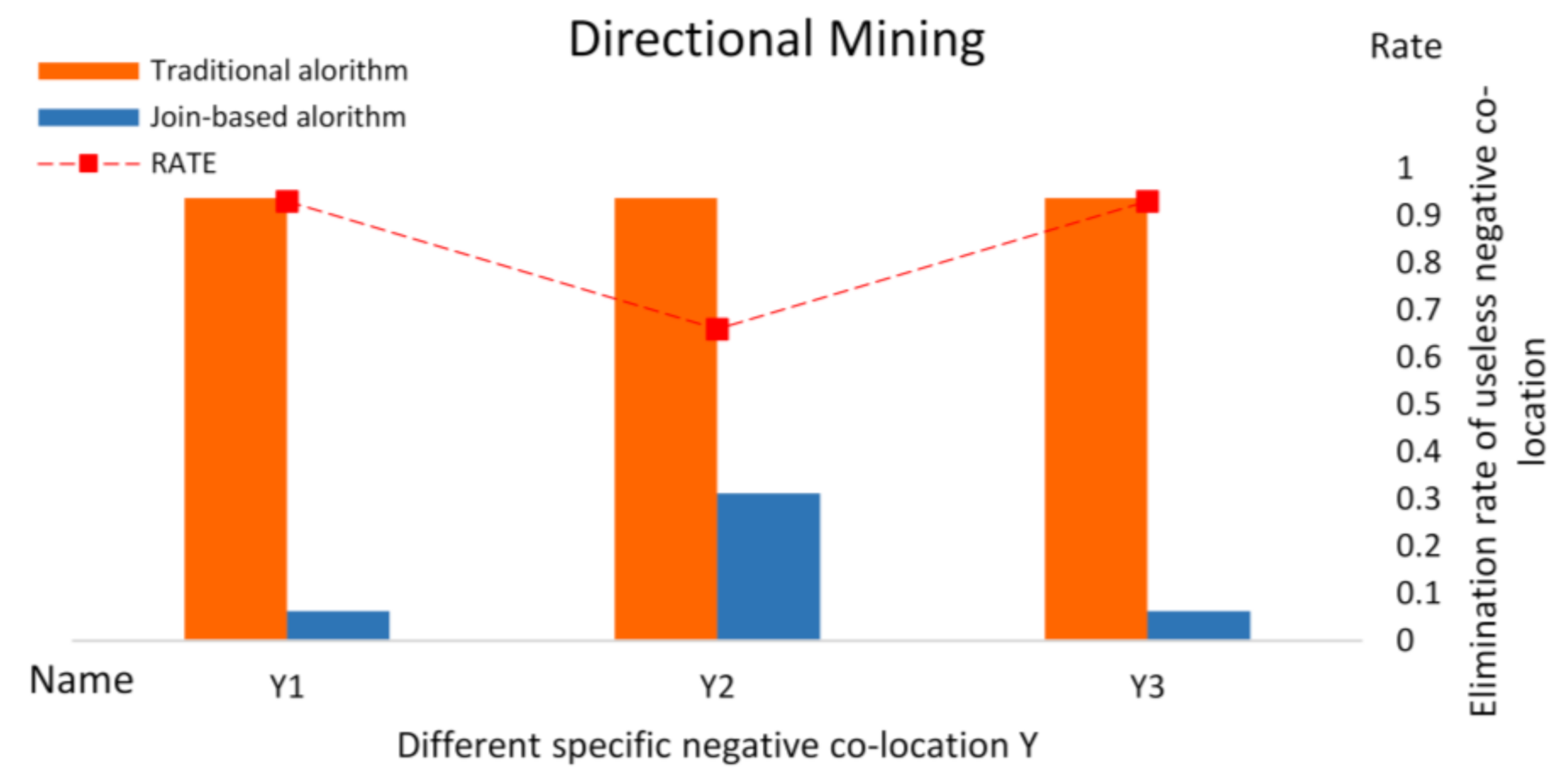
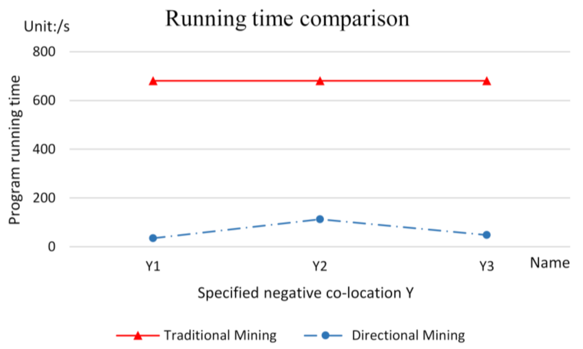
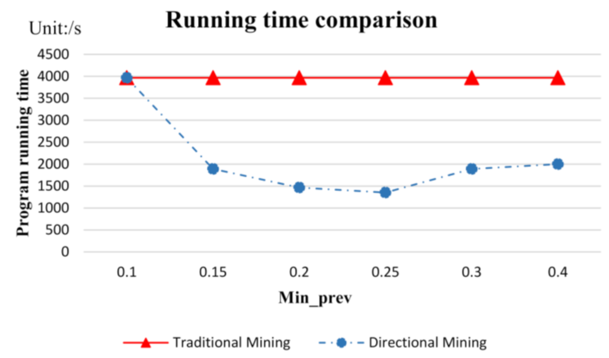
4.3. Experiment-1 with Join-Based Prevalent Negative Co-Location Pattern Directional Mining Algorithm

In this section, the experiment was carried out for directional mining with min_prev = 0.3 and different specified Y and SZs. And the results are shown in Figure 8 and Figure 9. The efficiency of filtering useless negative C-LP and the amounts of computation required by the different algorithms were compared. This experiment aimed to determine the number and filtration rate of candidate negative C-LP of Y 1 = S H O P ,   Y 2 = S H O P , T R A F F I C , Y 3 = T R A F F I C ,   DINING   R O O M , C O M P A N Y .
In the experiment of this section, we compared the calculation amount required for a certain number of frequent negative C-LP under the same features. Additionally, we also made a comparison between the calculation time of the algorithm proposed in Section 3 and the traditional algorithm. The traditional algorithm cannot cope with the change of Y . It can only calculate all the negative C-LP to obtain prevalent negative C-LP. So, its time and computational complexity were not affected by Y . Traditional algorithms are not directional. We can clearly see that the original algorithm could only calculate each negative C-LP and then compare min_prev. Therefore, the J-B algorithm can connect directly and save considerable time.

4.4. Experiments with Real Data-2

As shown in Table 3, to further validate the performance of the algorithm proposed in this paper, the real data, kindergartens, automobile services, restaurants, shops and Guilin per capita income, which include 1466 kindergartens, 1193 automobile services, 4202 restaurants and 473 shops, were used. According to the nature of the schools, kindergartens were classified into four types: public, private, public institutions and local businesses. The number of teachers and the size of the kindergarten were judged according to the number of classes and degrees in the kindergarten. In this paper, the per capita income of Guilin was divided as follows according to the “Guilin per capita disposable income from January to September 2021” issued by the Guilin Statistics Bureau of Guangxi Province. For urban personnel, a monthly income of more than 3500 RMB is rich, a monthly income of 3300~3500 RMB is medium and a monthly income of less than 3300 RMB is poor. For rural people, a monthly income of more than 1400 RMB is rich, a monthly income of 1100~1400 RMB is medium and an income of less than 1100 RMB is poor.
Because the number of some kindergarten types was small, the co-location PI and negative co-location PI for kindergartens in special data analysis were the PI values of the spatial features for kindergartens and were not the minimum values in the co-location pattern. The experiments were conducted to compare the performance of algorithms with spatial analysis by setting different thresholds of min_prev.
  • Algorithm performance analysis
This section analyzes the performance of the algorithm. Figure 10 show the comparison between our algorithm and the traditional algorithm, in which the broken line Rate represents the elimination rate of the useless co-location in the traditional algorithm by our algorithm, and the histogram is the calculation amount of each algorithm. It can be analyzed from Figure 10 that in this experiment, the elimination rate of the algorithm in this paper increased first and then decreased with the increase of the min_prev value. It can be seen that when min_prev was 0.25, the elimination rate was the largest, which was 0.7. It can be seen from Figure 11 that in this group of experimental data, the algorithm running time decreased first and then increased with the increase of min_prev. When min_prev was 0.25, the running time was the shortest, which was 1437 s. Through the experiments in this section, it was proved once again that our algorithm is faster than the traditional algorithm [49] and reduces the operation of useless negative co-location.
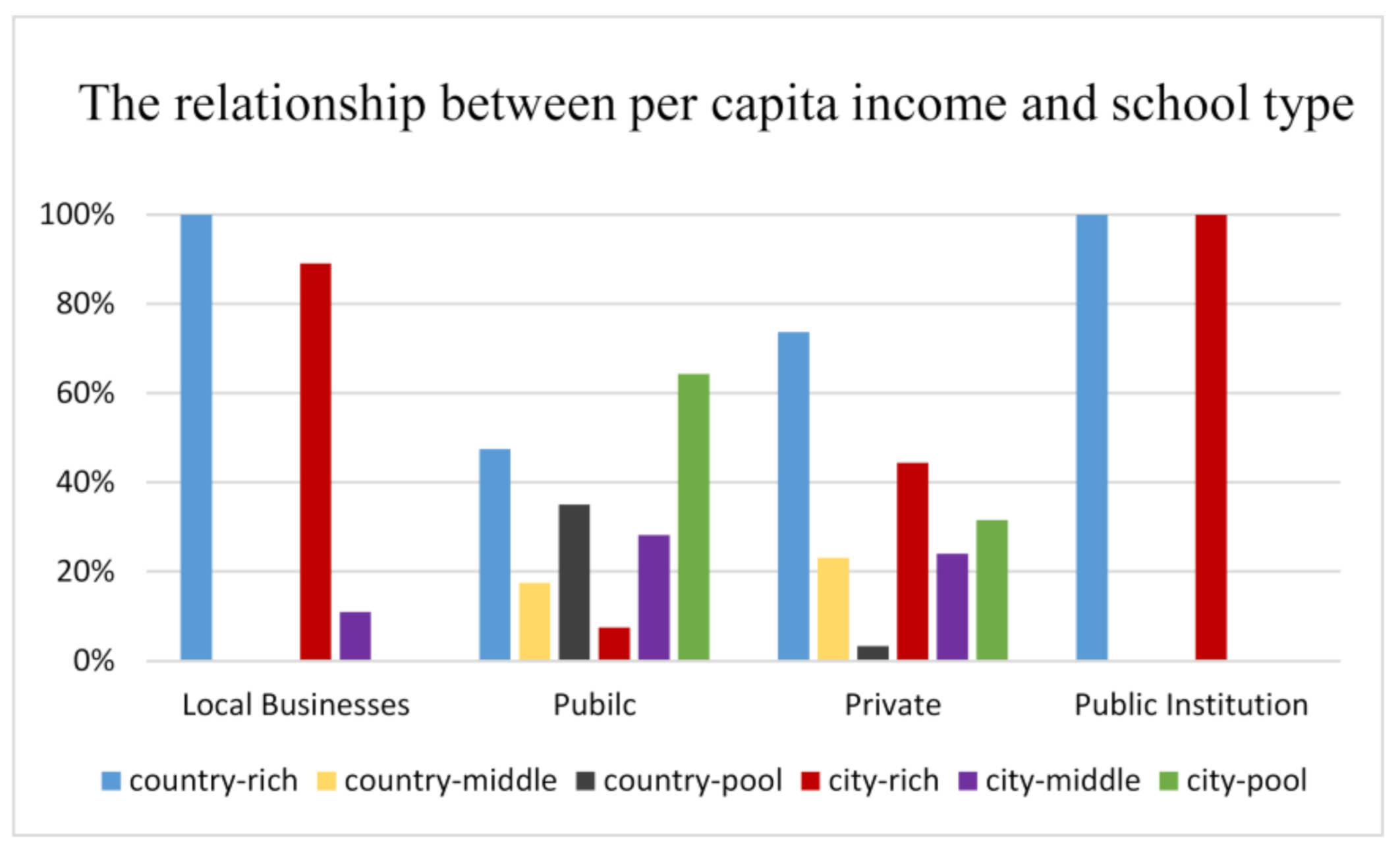
  • Spatial co-location analysis
This section conducts a spatial analysis of co-location PI values and negative co-location PI values for different types of kindergartens and the surrounding spatial features in Guilin. The analysis revealed the relationship between PI value and the size of kindergartens, as well as the economic situation of kindergarten families. The result is shown in Figure 12. As observed in Figure 12, the spatial analysis for private and public kindergartens is as follows:
(1) The PI value for the total co-location pattern F 0 = { private and public kindergarten, restaurant, shop, automobile service} is 0.11, and the PI value for the total negative co-location pattern F 0 = { private and public kindergarten, restaurant , shop ,   automobile   service } is 0.89. The negative co-location PI value is large, indicating that its mutual exclusion is greater than its correlation, showing that private and public kindergartens are widely distributed. In order to meet the schooling needs of most families, whether the surrounding environment of the kindergarten is prosperous is not the focus of the construction of private and public kindergartens.
(2) The size 2 co-location PI values for F 1 = { private and public kindergarten, restaurant},   F 2 = { private and public kindergarten, shop}, F 3 = { private and public kindergarten, automobile service} are 0.28, 0.17 and 0.21. Additionally, the negative co-location PI values for private and public schools F 1 = { private and public kindergarten,   restaurant   }, F 2 = { private and public kindergarten, shop }, F 3 = { private and public kindergarten, automobile   service } are 0.72, 0.83 and 0.79. The total negative co-location PI value may be too large because one of the features is mutually exclusive. By analyzing the size 2 negative co-location PI value, it can be seen that private and public kindergartens have no strong correlation with the surrounding features, indicating that their geographical location is indeed not very good, which is consistent with the conclusion of the total negative co-location.
(3) The co-location PI value and negative co-location PI value for the kindergarten and the surrounding features also discover the relationship between the size of the kindergarten and the economic status of students’ families. For example, the average number of private and public kindergarten classes is 5.38, and the average number of degrees is 139.13. This shows that there are fewer teachers and students in the kindergarten, which is consistent with the high negative co-location value (negative C-LPI: 0.89). Similarly, it can be seen from Figure 13 that in the family income of private and public kindergartens, poor families account for the highest proportion of 60%. The PI value of negative co-location is high, and the schools’ geographical location is not good; therefore, the families of the nearby schools are not wealthy, and teachers and students are scarce.
As observed in Figure 12, the spatial analysis for local business kindergartens is as follows:
(1) The PI value for the total co-location pattern F 0 = { local business kindergarten, restaurant, shop, automobile service} is 0.66, and the PI value for the total negative co-location pattern F 0 = { local business kindergarten, restaurant , shop ,   automobile   service } is 0.34. The negative co-location PI value for local business kindergartens is significantly lower than private and public kindergartens (negative C-LPI: 0.89), indicating that it has a good correlation with the surrounding spatial features. It shows that local businesses often build their own kindergartens next to business districts with better environments.
(2) The size 2 co-location PI value for local business kindergartens F 1 = { local business kindergarten, restaurant}, F 2 = { local business kindergarten, shop}, F 3 = { local business kindergarten, automobile service} are 0.88, 0.82 and 0.82. Additionally, the negative co-location PI value for local business kindergartens F 1 = { local business kindergarten,   restaurant   }, F 2 = { local business kindergarten, shop }, F 3 = { local business kindergarten, automobile   service } are 0.12, 0.18 and 0.18. From the size 2 co-location and negative co-location, it can be seen that the local business school has a good correlation with the surrounding spatial features, which is consistent with the total negative co-location.
(3) The average number of local business kindergarten classes is 11.17, and the average number of degrees is 316. Both of them are higher than public and private kindergartens (classes: 5.38, degrees: 139.13), indicating that there are many teachers and students in local business kindergartens, and the size of the kindergarten is large. Additionally, its negative co-location PI value of 0.34 is also smaller than public and private kindergartens (negative C-LPI: 0.89). This reveals that the smaller the negative co-location PI value, the larger the school size and the larger number of teachers and students. It can be seen from Figure 13 that 90% of the household economic income for local business kindergartens are high-income groups, and 10% are middle-income groups. This indicates that the smaller the negative co-location PI, the better the location of the kindergarten and the more affluent families that attend kindergartens nearby.
As observed in Figure 12, the spatial analysis for public institution kindergartens is as follows:
(1) The PI value for the total co-location pattern F 0 = { public institution kindergarten, restaurant, shop, automobile service} is 0.58, and the PI value for the total negative co-location pattern F 0 = { public institution kindergarten, restaurant , shop ,   automobile   service } is 0.42. The negative co-location PI value for public institution kindergarten is less than 0.5, indicating that its correlation with surrounding spatial features is greater than mutual exclusion. The kindergartens of public institutions are basically affiliated schools of universities, which is in good correlation with spatial features such as shops and restaurants.
(2) The size 2 co-location PI values for public institution kindergartens F 1 = { public institution kindergarten, restaurant}, F 2 = { public institution kindergarten, shop}, F 3 = { public institution kindergarten, automobile service} are 0.75, 0.58 and 0.58. Additionally, the negative co-location PI values for public institution kindergartens F 1 = { public institution kindergarten,   restaurant   }, F 2 = { public institution kindergarten, shop }, F 3 = { public institution kindergarten, automobile   service } are 0.25, 0.42, 0.42. The size 2 negative co-location PI value for public institution kindergartens is higher than local business kindergartens (negative C-LPI: 0.34) and lower than public and private kindergartens (negative C-LPI: 0.89). This is because although there are many restaurants and shops near the kindergarten affiliated with the university, it is not as numerous and dense as the kindergartens around the business district.
(3) The average number of classes in public institution kindergartens is 8.33, and the average number of degrees is 244.83. Both of them are higher than public and private kindergartens (classes: 5.38, degrees: 139.13) and lower than local business kindergartens (classes: 11.17, degrees: 316). Therefore, the number of the kindergartens’ students is “local business’s number > public institution’s number > number of private and public”, which is inversely proportional to the negative co-location PI value (each negative C-LPI: 0.34, 0.42 and 0.89). However, it is shown that the high-income families account for 100% of the household income for the kindergartens in public institutions in Figure 13, which is higher than local business kindergartens (high-income family: 90%). According to the negative co-location PI value (local business: 0.39, public institution: 0.42), it should be that the family income of local business kindergartens is higher than public institutions. This is because some low-level employees’ children in the local business also study in the school, but the staff and teachers in the university are basically senior intellectuals and have higher incomes.
Based on the above analysis, it can be seen that the lower the negative co-location PI value of the kindergarten and its surrounding features, the more prosperous the kindergarten is located, the more teachers and students the kindergarten has and the better the economic conditions of the family.

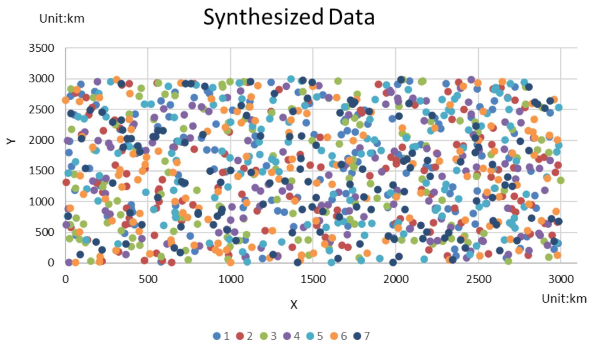
4.5. Experiments and Analysis with Synthetic Data Sets

As shown in Figure 14, in the experiment on the synthetic data set, the data set is seven sets generated by random numbers, and the total number of instances is 1000.
In this experiment section, the fixed distance threshold d = 150, and the participation threshold min_prev vary from 0.55 to 0.7. Since the experimental data are a random generation number, the data points are too random to generate a high-order negative C-LP. Therefore, this experiment is conducted on the SZ 3 negative C-LP. For example, the C-LP T = 0 , 1 , 2 . PI value of set 0 is 0.319, the PI value of set 1 is 0.248 and the PI value of the set is 0.207. Set the threshold min_prev = 0.5. For any negative C-LP generated by T, such as R = 0 , 1 , 2 and F = 0 , 1 , 2 , it must not satisfy the (1) of definition 3, and cannot become the prevalent negative C-LP, so we can just throw it out. However, traditional algorithms cannot deal with that, so they do a lot of useless calculations. With the change of the participation threshold, the number of candidate negative C-LPs mined by Algorithm 1 and the number of candidate negative C-Ls mined by the traditional algorithm are shown in Figure 15. When the threshold changes, the traditional method does not respond to it, and the algorithm starts filtering out the useless negative C-LP. When participation reaches 0.7, it is impossible to generate prevalent negative C-LP, but the traditional algorithm still needs to calculate all the PI values in the 198 PT to reach this conclusion. The curve above represents the actual number of prevalent negative C-LP.
The filtering rate of Algorithm 1 for the prevalent negative C-LP in the traditional algorithm is shown in Figure 15 and Figure 16. In Figure 15 the blue bar chart shows the number of candidates and useless negative C-LP required to calculate all the negative C-Ls under the set threshold. The orange bar chart shows the number of excluded PTs compared to the amount of computation required by traditional algorithms. The PI rate of the data in this randomized experiment is too dense, so the filtering rate can reach 100%, but there may be some differences in the actual situation.

5. Conclusions

To obtain the prevalent negative co-location pattern quickly and effectively, this paper proposes a join-based algorithm to mine them. Firstly, the algorithm mines the candidate negative co-location patterns at each size and then combines them with size 2 prevalent co-location patterns. This method can generate size n candidate negative co-location patterns by combining size n − 1 candidate negative co-location patterns with size 2 prevalent co-location patterns. The join-based method can avoid a lot of calculations for useless negative co-location patterns by combining each of them. Finally, the prevalent negative co-location patterns can be obtained by eliminating a small number of useless candidate negative co-location patterns.
From the experimental results, the following conclusions can be drawn up. The proposed algorithm, which calculates prevalent negative co-location patterns, is 30% faster than the traditional algorithm. Additionally, the algorithm reduces the calculations for useless negative co-location patterns by an average of about 40% relative to the traditional algorithm.
Although our method can mine prevalent negative co-location patterns effectively, it cannot perform an analogy for those similar negative co-location patterns with different spatial features. It is hopeful that we can solve this problem by adding convolution into the algorithm in the future.

Author Contributions

Conceptualization, G.Z. and Z.W.; methodology, Z.W.; software, G.Z.; validation, Q.L.; formal analysis, Z.W.; investigation, G.Z.; resources, G.Z.; data curation, G.Z.; writing—original draft preparation, G.Z.; writing—review and editing, G.Z.; visualization, G.Z.; supervision, Q.L.; project administration, Z.W.; funding acquisition, G.Z. All authors have read and agreed to the published version of the manuscript.

Funding

This paper is financially supported by the National Natural Science of China (Project No. 41961065), Guangxi Science and Technology Base and Talent Project (Project No. GuikeAD19254002, GuikeAA18118038 and GuikeAA18242048), Guangxi Natural Science for Innovation Research Team (Project No. 2019GXNSFGA245001), Guilin Research and Development Plan Program (Project No. 20190210-2), the National Key Research and Development Program of China (Project No. 2016YFB0502501), the BaGuiScholars program of Guangxi (Guoqing Zhou), Innovation Project of Guangxi Graduate Education (Project No. YCBZ2021061) and Guangxi Key Laboratory of Spatial Information and Geomatics Program (Project No. 19-050-11-14).

Conflicts of Interest

The authors declare no conflict of interest.

References

  1. Morimoto, Y. Mining Frequent Neighboring Class Sets in Spatial Databases. In Proceedings of the seventh ACM SIGKDD International Conference on Knowledge Discovery and Data Mining, San Francisco, CA, USA, 26 August 2001; pp. 353–358. [Google Scholar]
  2. Shekhar, S.; Huang, Y. Co-location Rules Mining: A Summary of Results. In Proceedings of the International Symposium on Spatio and Temporal Database (SSTD’01), Redondo Beach, CA, USA, 12–15 July 2001; Springer: Berlin/Heidelberg, Germany; pp. 236–240. [Google Scholar]
  3. Huang, Y.; Shekhar, S.; Xiong, H. Discovering colocation patterns from spatial data sets: A general approach. IEEE Trans. Knowl. Data Eng. 2004, 16, 1472–1485. [Google Scholar] [CrossRef] [Green Version]
  4. Yoo, J.S.; Shekhar, S.; Smith, J.; Kumquat, J.P. A partial join approach for mining co-location patterns. In Proceedings of the 12th Annual ACM International Workshop on Geographic Information Systems (GIS), Washington, DC, USA, 12–13 November 2004; ACM Press: New York, NY, USA, 2004; pp. 241–249. [Google Scholar]
  5. Yoo, J.S.; Shekhar, S.; Celik, M. A join-less approach for co-location pattern mining: A summary of results. In Proceedings of the IEEE International Conference on Data Mining, Houston, TX, USA, 27–30 November 2005; IEEE Press: Piscataway, NJ, USA, 2005; pp. 813–816. [Google Scholar]
  6. Wang, L.; Bao, Y.; Lu, J.; Yip, J. A New Join-less Approach for Co-location Pattern Mining. In Proceedings of the IEEE 8th International Conference on Computer and Information Technology (CIT2008), Sydney, NSW, Australia, 8–11 July 2008; pp. 197–202. [Google Scholar]
  7. Wang, L.; Bao, Y.; Lu, Z. Efficient discovery of spatial co- location patterns using the iCPI-tree. Open Inf. Syst. J. 2009, 3, 69–80. [Google Scholar] [CrossRef] [Green Version]
  8. Djenouri, Y.; Lin, C.W.; Nrvg, K.; Ramampiaro, H. Highly Efficient Pattern Mining Based on Transaction Decomposition. In Proceedings of the IEEE 35th International Conference on Data Engineering (ICDE), Macao, China, 8–11 April 2019. [Google Scholar]
  9. Xun, Y.; Zhang, J.; Qin, X.; Zhao, X. FiDoop-DP: Data partitioning in frequent itemset mining on Hadoop clusters. IEEE Trans. Parallel Distrib. Syst. 2017, 28, 101–114. [Google Scholar] [CrossRef]
  10. Djenouri, Y.; Comuzzi, M. Combining apriori heuristic and bioinspired algorithms for solving the frequent itemsets mining problem. Inf. Sci. 2017, 420, 1–15. [Google Scholar] [CrossRef]
  11. Deng, Z.-H.; Lv, S.-L. PrePost+: An efficient n-lists-based algorithm for mining frequent itemsets via children—Parent equivalence pruning. Expert Syst. Appl. 2015, 42, 5424–5432. [Google Scholar] [CrossRef]
  12. Djenouri, Y.; Djenouri, D.; Lin, J.C.-W.; Belhadi, A. Frequent itemset mining in big data with effective single scan algorithms. IEEE Access 2018, 6, 68013–68026. [Google Scholar] [CrossRef]
  13. Zhang, B.; Lin, J.C.-W.; Shao, Y.; Fournier-Viger, P.; Djenouri, Y. Maintenance of Discovered High Average-Utility Itemsets in Dynamic Databases. Appl. Sci. 2018, 8, 769. [Google Scholar] [CrossRef] [Green Version]
  14. Deng, Z.H.; Lv, S.L. Fast mining frequent itemsets using nodesets. Expert Syst. Appl. 2014, 41, 4505–4512. [Google Scholar] [CrossRef]
  15. Yao, H.; Hamilton, H.J.; Butz, C.J. A foundational approach to mining itemset utilities from databases. In Proceedings of the SIAM International Conference on Data Mining, Lake Buena Vista, FL, USA, 22–24 April 2004; pp. 215–221. [Google Scholar]
  16. Lan, G.C.; Hong, T.P.; Huang, J.P.; Tseng, V.S. On-shelf utility mining with negative item values. Expert Syst. Appl. 2014, 41, 3450–3459. [Google Scholar] [CrossRef]
  17. Liu, J.; Wang, K.; Fung, B.C.M. Direct discovery of high utility itemsets without candidate generation. In Proceedings of the IEEE International Conference on Data Mining, Brussels, Belgium, 10–13 December 2012; pp. 984–989. [Google Scholar]
  18. Bao, X.; Wang, L. A clique-based approach for co-location pattern mining. Inf. Sci. 2019, 490, 244–264. [Google Scholar] [CrossRef]
  19. Wang, L.; Zhou, L.; Lu, J.; Yip, Y.J. An order-clique-based approach for mining maximal co-locations. Inf. Sci. 2009, 179, 3370–3382. [Google Scholar] [CrossRef]
  20. Celik, M.; Kang, J.M.; Shekhar, S. Zonal Co-location Pattern Discovery with Dynamic Parameters. In Proceedings of the Seventh IEEE International Conference on Data Mining (ICDM 2007), Omaha, NE, USA, 28–31 October 2007. [Google Scholar]
  21. Yu, C. A Review of Spatial Co-location Pattern Mining Algorithms. Comput. Digit. Eng. 2014, 42, 6. [Google Scholar]
  22. Wang, L.; Bao, X.; Chen, H.; Cao, L. Effective lossless condensed representation and discovery of spatial co-location patterns. Inf. Sci. 2018, 436–437, 197–213. [Google Scholar] [CrossRef]
  23. Wang, L.; Bao, X.; Zhou, L. Redundancy reduction for prevalent co-location patterns. IEEE Trans. Knowl. Data Eng. 2018, 30, 142–155. [Google Scholar] [CrossRef]
  24. Hu, X.; Wang, L.; Zhou, L.; Wen, F. Mining Spatial Maximal Co-Location Patterns. J. Front. Comput. Sci. Technol. 2014, 8, 150–160. [Google Scholar]
  25. Ouyang, Z.; Wang, L.; Chen, H. Research on Mining Spatial Co-location Pattern of Fuzzy Objects. Chin. J. Comput. 2011, 34, 1947–1955. [Google Scholar] [CrossRef]
  26. He, F.; Jia, Z.; Zhang, D. Mining spatial co-location pattern based on parallel computing. J. Yunnan Norm. Univ. (Nat. Sci. Ed.) 2015, 35, 56–62. [Google Scholar]
  27. Zhou, G.; Wang, L. Co-location decision tree for enhancing decision-making of pavement maintenance and rehabilitation. Transp. Res. Part C 2011, 21, 287–305. [Google Scholar] [CrossRef] [Green Version]
  28. Zhou, G.; Zhang, R.; Zhang, D. Manifold Learning Co-Location Decision Tree for Remotely Sensed Imagery Classification. Remote Sens. 2016, 8, 855. [Google Scholar] [CrossRef] [Green Version]
  29. Zhou, G.; Li, Q.; Deng, G. Maximal Instance Algorithm for Fast Mining of Spatial Co-Location Patterns. Patterns. Remote Sens. 2021, 13, 960. [Google Scholar] [CrossRef]
  30. Zhou, G. Data Mining for Co-location Pattern: Theory and Application; Taylor & Francis: Oxfordshire, UK; CRC Press: Boca Raton, FL, USA, 2021; 212p, ISBN 978-03-67-654269. [Google Scholar]
  31. Zhou, G.; Huang, S.; Wang, H.; Zhang, R.; Wang, Q.; Sha, H.; Liu, X.; Pan, Q. A buffer analysis based on co-location algorithm. ISPRS Int. Arch. Photogramm. Remote Sens. Spat. Inf. Sci. 2018, XLII-3, 2487–2490. [Google Scholar] [CrossRef] [Green Version]
  32. Zhou, G.; Li, Q.; Deng, G.; Yue, T.; Zhou, X. Mining co-location patterns with clustering items from spatial data sets. ISPRS Int. Arch. Photogramm. Remote Sens. Spat. Inf. Sci. 2018, XLII-3, 2505–2509. [Google Scholar] [CrossRef] [Green Version]
  33. Zhou, G.; Zhou, X.; Yang, J.; Tao, Y.; Nong, X.; Baysal, O. Flash Lidar Sensor using Fiber Coupled APDs. IEEE Sens. J. 2015, 15, 4758–4768. [Google Scholar] [CrossRef]
  34. Zhou, G.; Yue, T.; Huang, Y.; Song, B.; Chen, K.; He, G.; Ni, G.; Zhang, L. Study of an SCSG-OSM for the Creation of an Urban Three-Dimensional Building. IEEE Access 2020, 8, 126266–126283. [Google Scholar] [CrossRef]
  35. Zhang, R.; Zhou, G.; Huang, J.; Zhou, X. Maximum Variance Unfolding Based Co-Location Decision Tree for Remote Sensing Image Classification. In Proceedings of the 2017 IEEE International Geoscience and Remote Sensing (IGARSS), Fort Worth, TX, USA, 23–28 July 2017. [Google Scholar]
  36. Zhou, G. Urban High-Resolution Remote Sensing: Algorithms and Modelling; Taylor & Francis: Oxfordshire, UK; CRC Press: Boca Raton, FL, USA, 2020; 465p, ISBN 978-03-67-857509. [Google Scholar]
  37. Wu, X.; Zhang, C.; Zhang, S. Efficient mining of both positive and negative association rules. ACM Trans. Inf. Syst. 2004, 22, 381–405. [Google Scholar] [CrossRef]
  38. Zheng, Z.; Zhao, Y.; Zuo, Z.; Cao, L. Negative-GSP: An efficient method for mining negative sequential patterns. In Proceedings of the Eighth Australasian Data Mining Conference, Melbourne, Australia, 1 December 2009; ACM Press: New York, NY, USA, 2009; pp. 63–67. [Google Scholar]
  39. Cao, L.; Dong, X.; Zheng, Z. e-NSP: Efficient negative sequential pattern mining. Artif. Intell. 2016, 235, 156–182. [Google Scholar] [CrossRef] [Green Version]
  40. Cao, L. In-depth behavior understanding and use: The behavior informatics approach. Inf. Sci. 2010, 180, 3067–3085. [Google Scholar] [CrossRef]
  41. Cao, L.; Zhao, Y.; Zhang, C. Mining impact-targeted activity patterns in imbalanced data. IEEE Trans. Knowl. Data Eng. 2008, 20, 1053–1066. [Google Scholar] [CrossRef]
  42. Dong, X.; Zhao, L.; Han, X.; Jiang, H. Comparisons of several definitions about negative containment. In Proceedings of the ICCNT’ 11, Harbin, China, 24–26 December 2011; pp. 553–556. [Google Scholar]
  43. Zheng, Z.; Zhao, Y.; Zuo, Z.; Cao, L. An efficient ga-based algorithm for mining negative sequential patterns. In Advances in Knowledge Discovery and Data Mining; PAKDD 2010; Lecture Notes in Computer Science; Springer: Berlin/Heidelberg, Germany, 2010; Volume 6118, pp. 262–273. [Google Scholar]
  44. Dong, X.; Gong, Y.; Cao, L. F-NSP+: A fast negative sequential patterns mining method with self-adaptive data storage. Pattern Recognit. 2018, 84, 13–27. [Google Scholar] [CrossRef]
  45. Rastogi, V.; Khare, V.K. Apriori Based: Mining Positive and Negative Frequent Sequential Patterns. Int. J. Latest Trends Eng. Technol. (IJLTET) 2012, 1, 24–33. [Google Scholar]
  46. Khare, V.K.; Rastogi, V. Mining Positive and Negative Sequential Pattern in Incremental Transaction Databases. Int. J. Comput. Appl. 2013, 71, 18–22. [Google Scholar]
  47. Mesbah, S.; Taghiyareh, F. A new sequential classification to assist Ad auction agent in making decisions. In Proceedings of the 2010 5th International Symposium on Telecommunications (IST), Kish Island, Iran, 4–6 December 2010; pp. 1006–1012. [Google Scholar]
  48. Schwartz, G.W.; Shokoufandeh, A.; Ontan, S.; Hershberg, U. Using a novel clumpiness measure to unite data with metadata: Finding common sequence patterns in immune receptor germline V genes. Pattern Recognit. Lett. 2016, 74, 24–29. [Google Scholar] [CrossRef]
  49. Jiang, Y.; Wang, L.; Lu, Y.; Chen, H. Discovering both positive and negative co-location rules from spatial data sets. In Proceedings of the 2nd International Conference on Software Engineering and Data Mining, Chengdu, China, 23–25 June 2010; IEEE Press: Piscataway, NJ, USA, 2010; pp. 398–403. [Google Scholar]
  50. Wang, G.; Wang, L.; Yang, P.; Chen, H. Minimal negative Co-location model and Effective Mining Algorithm. Comput. Sci. Explor. 2021, 15, 366. [Google Scholar]
Figure 1. Spatial negative co-location example.
Remotesensing 14 02103 g001
Figure 2. Join-based algorithm with a connect example.
Remotesensing 14 02103 g002
Figure 3. Join-based algorithm with a complete example.
Remotesensing 14 02103 g003
Figure 4. The position of each feature in Jinan is displayed.
Remotesensing 14 02103 g004
Figure 5. The number of JINAN positive C-LP.
Remotesensing 14 02103 g005
Figure 6. A comparison between the negative C-LP algorithm based on the J-B and traditional algorithms with the change in threshold value.
Remotesensing 14 02103 g006
Figure 7. The relationship between the ratio of the number of positive and negative PT and the pruning rate.
Remotesensing 14 02103 g007
Figure 8. A comparison between the negative C-LP algorithm based on the J-B and traditional algorithms with the change in Y and SZ.
Remotesensing 14 02103 g008
Figure 9. Comparison of running times between traditional mining and directional mining under different numbers of features.
Remotesensing 14 02103 g009
Figure 10. A comparison between the negative C-LP algorithm based on the J-B and traditional algorithms with the change in threshold value (experiment-2).
Remotesensing 14 02103 g010
Figure 11. Comparison of running times between traditional mining and directional mining under different Min_prev.
Remotesensing 14 02103 g011
Figure 12. Different school types of the value of PI.
Remotesensing 14 02103 g012
Figure 13. The relationship between per capita income and school type.
Remotesensing 14 02103 g013
Figure 14. Synthetic data used to detect the generality of the algorithm. In the figure, random numbers are used to generate 7 sets of coordinates that are irregular.
Remotesensing 14 02103 g014
Figure 15. The traditional algorithm and the J-B negative C-L algorithm need to calculate the comparison between the number of PT and the actual negative C-LP.
Remotesensing 14 02103 g015
Figure 16. Filtration rate of connection algorithm for useless negative C-LP.
Remotesensing 14 02103 g016
Table 1. Abbreviation explanation.
TermsAbbreviationDefinition
Co-locationC-LCo-location is two spatial feature instances that satisfy R (e.g., Euclidean distance metric). [2]
Co-location patternC-LPThe co-location pattern is the co-location combination of spatial instance S   =   s 1 , s 2 , s 3 , , s n satisfying R in a given spatial feature F   =   f 1 , f 2 , f 3 , , f n . [2]
The PI value of the C-LPC-LPIIn this paper, the C-LPI is the value of the participation index for the co-location pattern.
PatternPTIn this paper, the pattern represents a specific spatial instance co-location relationship.
Participation IndexPIThe participation index (PI) of a co-location c   =   f 1 , f 2 , f 3 , , f n . [49]
The value of the participation indexTVPIThe value of the participation index is the minimum in all PR (c, , f k ) of co-location C. [49]
SizeSZIn this paper, size is the number of spatial feature sets F   =   f 1 , f 2 , f 3 , , f n .
Co-location of SizeC-LSZCo-location of size is the number of spatial feature sets F   =   f 1 , f 2 , f 3 , , f n . [2]
Table 2. In the real data, the number and category of 4 kinds of features.
TypeAbbreviationNumber
ShoppingS7284
TrafficT582
Dining RoomD1963
CompaniesC1360
Table 3. In the real data, the number and category of 4 kinds of features.
TypeAbbreviationNumber
SchoolS1466
Automobile ServiceA1193
RestaurantR4202
ShopSP473
Publisher’s Note: MDPI stays neutral with regard to jurisdictional claims in published maps and institutional affiliations.

