Computationally Efficient Implementation of Joint Detection and Parameters Estimation of Signals with Dispersive Distortions on a GPU

Abstract

The detector is an integral part of the device for receiving and processing radio signals. Signals that have passed through the ionospheric channel acquire an unknown Doppler shift and are subject to dispersion distortions. It is necessary to carry out joint detection and parameter estimation to improve reception quality and detection accuracy. Modern hardware base developing makes it possible to implement a device for joint detection and evaluation of signals based on standard processors (CPU) and graphic processors (GPU). The article discusses the implementation of a signal detector that allows for real-time operation. A comparison of implementations of algorithms for estimating the Doppler frequency shift through multiplication by a complex exponent and the fast Fourier transform (FFT) is performed. A comparison of computational costs and execution speed on the CPU and GPU is considered.

1. Introduction

Ionospheric radio communication is a highly reliable and cost-effective solution for organizing communication with outlying regions, as well as with regions whose infrastructure has been disrupted due to natural disasters. Currently, development of decameter ionospheric radio communication systems is on the way to increasing the speed of information transmission [1,2,3,4,5,6]. When using broadband signals in the decameter range, the frequency dispersion has a significant effect on the signal [7,8,9,10,11,12,13,14]. Thus, due to the frequency dispersion, at different frequencies wideband signals have different propagation delays. Such a difference leads to a synchronization error and affects the quality of signal detection and the quality of information reception [15,16,17]. A separate problem is the detection of long signal preambles with a duration of about several seconds long, with a spectrum wider than 100 kHz [18,19,20] and with a coherent accumulation of the detected signal energy throughout its duration. In this case, the signal base reaches a value exceeding 50 dB, and the required accuracy of estimation and compensation of the Doppler frequency shift is in the tenths and in some cases hundredths of a hertz. Otherwise, the coherent accumulation of signal energy over time intervals of units or even tens of seconds becomes impossible. Simultaneously, with the evaluation of the Doppler shift [21,22,23,24,25,26], it is also required to evaluate and compensate for the dispersion distortions of the detected signals.

In this paper, we show the possibility of constructing a device for the joint detection and estimation of the parameters of signals with dispersion distortions on graphic processors. Implementations proposed in this paper allow for the simultaneous detection of signals and estimation of dispersion distortions, delay, Doppler shift, and initial phase in real time.

2. Related Work

Stein, Tolimieri, and Winograd are the founders of research on algorithms for calculating uncertainty functions. Stein has described a processing approach for obtaining joint delay and frequency offset (DTO/DFO) estimates for continuous signals based on the efficient calculation of complex ambiguity functions [27]. Typically, it involves a two-mode process called coarse and fine modes. Coarse mode is used to greatly reduce the time delay and frequency offset uncertainty, after which fine mode calculations are performed. Precise mode uses product/filter mixing interpretation, greatly reducing the processing load. Tolimieri and Winograd proposed an algorithm for the discrete ambiguity function calculation in [28]. They rely on the fact that, in most basic applications, it is necessary to calculate the limited parts of the DFT of a discrete ambiguity function. To do this, they first pass a long sequence through a decimated FIR filter, and then they use the FFT algorithm. Additionally, computationally efficient algorithms for the joint estimation of the Doppler shift and time delay are considered in [29,30]. These papers propose a new method based on a pre-weighted Zoom FFT with a cascaded filter algorithm to minimize the processing load of cross-ambiguity functions without compromising performance. The weighting process in the Zoom FFT method provided an opportunity for the researchers to get rid of redundant calculations. The multi-stage filtering method was used to reduce complexity and to obtain a high-performance system. A method for processing segments was also proposed, adapted to calculate the ambiguity function when imposing input data frames. By considering the calculation of the cross-ambiguity functions of overlapping data frames as the calculation of the FFT of the overlapping data, the redundancy of the calculations can be eliminated.

Modern techniques for reducing the complexity of the cross-ambiguity function (CAF) are based on numerical fitting for CAF [31]. These algorithms make full use of the property that the CAF is symmetrical in the frequency domain. Simulation results show that, compared to the method that looks for the CAF peak, the proposed algorithm can significantly reduce computational complexity while meeting the accuracy requirements of the joint time-frequency estimate.

In paper [32], the authors propose a method for solving the problem of determining the mutual delay time of ultra-wideband signals. A modified algorithm, which can be implemented by parallel calculation of the cross-ambiguity function, was used to compensate Doppler shift of the recorded signals. This algorithm was based on the division of an ultra-wideband signal into separate frequency channels. An increase in the computational efficiency of the proposed algorithm was achieved by parallel calculation of the convolution function and cross-ambiguity.

However, all the above works do not take into account the problem of compensating for dispersion distortions and processing signals with a base over 50 dB. There are also no computationally efficient solutions implemented on the GPU that allow for the real-time detection of signals with a base of more than 50 dB (the signal spectrum width is hundreds of kHz, the duration is a few seconds) with the simultaneous estimation of dispersion distortions, delay, Doppler shift, and initial phase. Given these features, the joint detection and estimation of signal parameters requires large computational resources. The modern technology level makes it possible to consider the possibility of developing a computationally efficient implementation of various algorithms on GPUs. For example, such GPU implementation allows you to build systems for parallel simulation of MIMO radars [33] and build digital downconverter [34]. Additionally, GPUs are very often used in deep learning [35]. Thus, computing on GPUs is becoming more and more efficient.

3. Analytical Formulation of the Problem

The complex envelope of the signal at the joint detection and signal parameters estimation device input can be represented as a composition of the useful signal complex envelope, distorted by the frequency dispersion of ionospheric channel, and the complex envelope of white Gaussian noise:

$$\begin{array}{c}{\dot{y}}_i(\phi ,\tau =l\cdot \Delta t,f_d,s)=e^{-j\phi }{e}^{j2\pi f_d\left(i-l\right)\Delta t}{\dot{x}}_{i-l}\left(s\right)+{\dot{n}}_i,\\ i=0÷N_p-1,\end{array}$$

(1)

where $\dot{\overline{x}}\left(s\right)=\dot{\overline{x}}\ast \dot{\overline{h}}(s)$ is distorted by the ionospheric channel useful signal complex envelope, ${\dot{h}}_i\left(s\right)$ is the ionospheric channel impulse response (IR) complex envelope, ${\dot{x}}_i$ is the complex envelope of useful undistorted signal, $f_d$ is the doppler frequency shift, $\tau$ is the delay in seconds, $l$ is the delay in samples, $\Delta t$ is the sample time, $s$ is the slope of the dispersion characteristic (parameter that characterizes dispersion distortions), $\phi$ is the unknown phase shift, $\dot{n}(t)$ is the complex envelope of white Gaussian noise with zero mean and variance ${\sigma }_{ɯ}^2$, and $N_p$ is the number of samples.

The ionospheric channel impulse response (IR) complex envelope connects with frequency response of the ionospheric channel $\dot{H}(j2\pi f)$ through Fourier transform $\dot{H}(j2\pi f)$:$\dot{h}\left(t,s\right)={\displaystyle \underset{-\infty }{\overset{\infty }{\int }}\dot{H}(j2\pi f)e^{j2\pi f}df}$, where $x\left(t\right)$ is a transmitted signal that is known at the receiving side.

The ionospheric channel model, which takes into account frequency dispersion, is proposed in [8]. We consider version of this model with a linear dispersion characteristic. Then frequency response of the ionospheric channel in the absence of multipath signal propagation can be described as

$$\dot{H}(j2\pi f)=e^{-j\pi s{f}^2},f\in \left[-\Delta f/2;\Delta f/2\right],$$

(2)

where $\Delta f$ is the bandwidth of the ionospheric channel.

The decision statistic can be found as:

$${\dot{\lambda }}_i(\phi ,\tau ,f_d,s)={\displaystyle \sum _{n=0}^{N_p-1}{\dot{y}}_n(\phi ,\tau =l\cdot \Delta t,f_d,s){\dot{g}}_{i-n}^{\ast }(f_d,s)},$$

(3)

where the matched filter impulse response $\dot{g}$ is defined as

$${\dot{g}}_{N_p-1-i}(f_d,s)={\displaystyle \sum _{n=0}^{N_p-1}{\dot{x}}_n{e}^{j2\pi f_{d}n\Delta t}{\dot{h}}_{i-n}^{\ast }(s)}.$$

(4)

Then, the parameter estimates can be found as:

$$\widehat{\phi },\widehat{\tau },\widehat{f_d},\widehat{s}=\underset{\phi ,\tau ,f_d,s}{\arg \max }{\dot{\lambda }}_i(\phi ,\tau ,f_d,s),$$

(5)

where $\widehat{\phi },\widehat{\tau },\widehat{f_d}$ and $\widehat{s}$ are estimates of $\phi ,\tau ,f_d$ and $s$, respectively.

4. Implementation of a Matched Filter

This section may be divided by subheadings. It should provide a concise and precise description of the experimental results, their interpretation, and the experimental conclusions that can be drawn. From Equation (2) it can be seen that the number of matched filters to obtain a complete set of decision statistics ${\dot{\lambda }}_i(\phi ,\tau ,f_d,s)$ is determined by the number of possible Doppler frequency shifts $f_d$ and slopes of the dispersion characteristic $s$:

$$N_{mf}=N_{f_d}{N}_s,$$

(6)

where $N_{mf}$ is the number of matched filters, $N_{f_d}$ is the number of possible Doppler frequency shifts $f_d$, and $N_s$ is the number of possible slopes of the dispersion characteristic $s$. A large number of matched filters imposes high requirements on the computing platform. Doppler frequency shift $f_d$ consideration (for its estimation) can be carried out after matched filtering, then Equation (2) can be represented as:

$${\dot{\lambda }}_i(\phi ,\tau ,f_d,s)=e^{j2\pi f_{d}i\Delta t}{\displaystyle \sum _{n=0}^{N_p-1}{\dot{y}}_n(\phi ,\tau =l\cdot \Delta t,f_d,s){\dot{g}}_{i-n}(s)},$$

(7)

where

$${\dot{g}}_{N_p-1-i}(s)={\displaystyle \sum _{n=0}^{N_p-1}{\dot{x}}_n{\dot{h}}_{i-n}^{\ast }(s)}.$$

(8)

The above transformation reduces number of required matched filters to $N_{mf}=N_s$, which can significantly reduce computational costs. However, in the conditions of an ionospheric channel, due to the presence of a Doppler frequency shift during the observation of the complex envelope at the input of the matched filter, a phase drift occurs, which leads to losses in the SNR at the output of the matched filter. To minimize these losses, we will convolve not with a reference signal of duration $N_p$, but with signals (see Figure 1):

$${\dot{x}}_{m,n}={\dot{x}}_{n+m\cdot N_{pp}},n=0÷N_{pp}-1,m=0÷M-1,$$

(9)

where $N_{pp}=\frac{N_p}{M}$, and $M$ is the number of splits of the original sequence.

In this case, matched filtering can be performed using a series-matched filter, which is a set of filters matched with sequences ${\dot{x}}_{m,n}$.

4.1. Estimation Algorithm via Complex Exponents

A filter matched with a series of sequences is shown at Figure 2. The signal at the output of each matched filter can be written as:

$${\dot{\lambda }}_{m,n}(s)={\displaystyle \sum _{l=0}^{N_{pp}-1}{\dot{y}}_{m,l}{\dot{g}}_{m,n-l}^{\ast }(s)},n=0÷N_{pp}-1,m=0÷M-1,$$

(10)

where ${\dot{g}}_{M-1-m,N_{pp}-1-n}(s)={\displaystyle \sum _{k=0}^{N_p-1}{\dot{x}}_{{}_{k+m{N}_{pp}}}{\dot{h}}_{n-(k+m{N}_{pp})}^{\ast }(s)}$ is the complex impulse response envelope of the filter matched to the $m$-th sequence.

Doppler frequency shift is taken into account:

$${\dot{\lambda }}_{m,n}(f_d,s)={\dot{\lambda }}_{m,n}(s)\cdot e^{j2\pi f_d(n+m{N}_{pp})\Delta t}.$$

(11)

The decision statistics at the matched filter output can be obtained as:

$${\dot{\lambda }}_n(f_d,s)={\displaystyle \sum _{m=0}^{M-1}{\dot{\lambda }}_{m,n}(f_d,s)}.$$

(12)

The interval of allowable values of the Doppler frequency shift is $\left[-\frac{f_s}{2N_{pp}}:\frac{f_s}{2N_{pp}}\right]$, where $f_s$ is the sample rate. Within this interval, value of the estimated Doppler frequency shift can be arbitrary. A significant drawback of this implementation is the requirement for the amount of RAM to store arrays with complex exponents.

Joint detection and signal parameters estimation device scheme is shown in Figure 3.

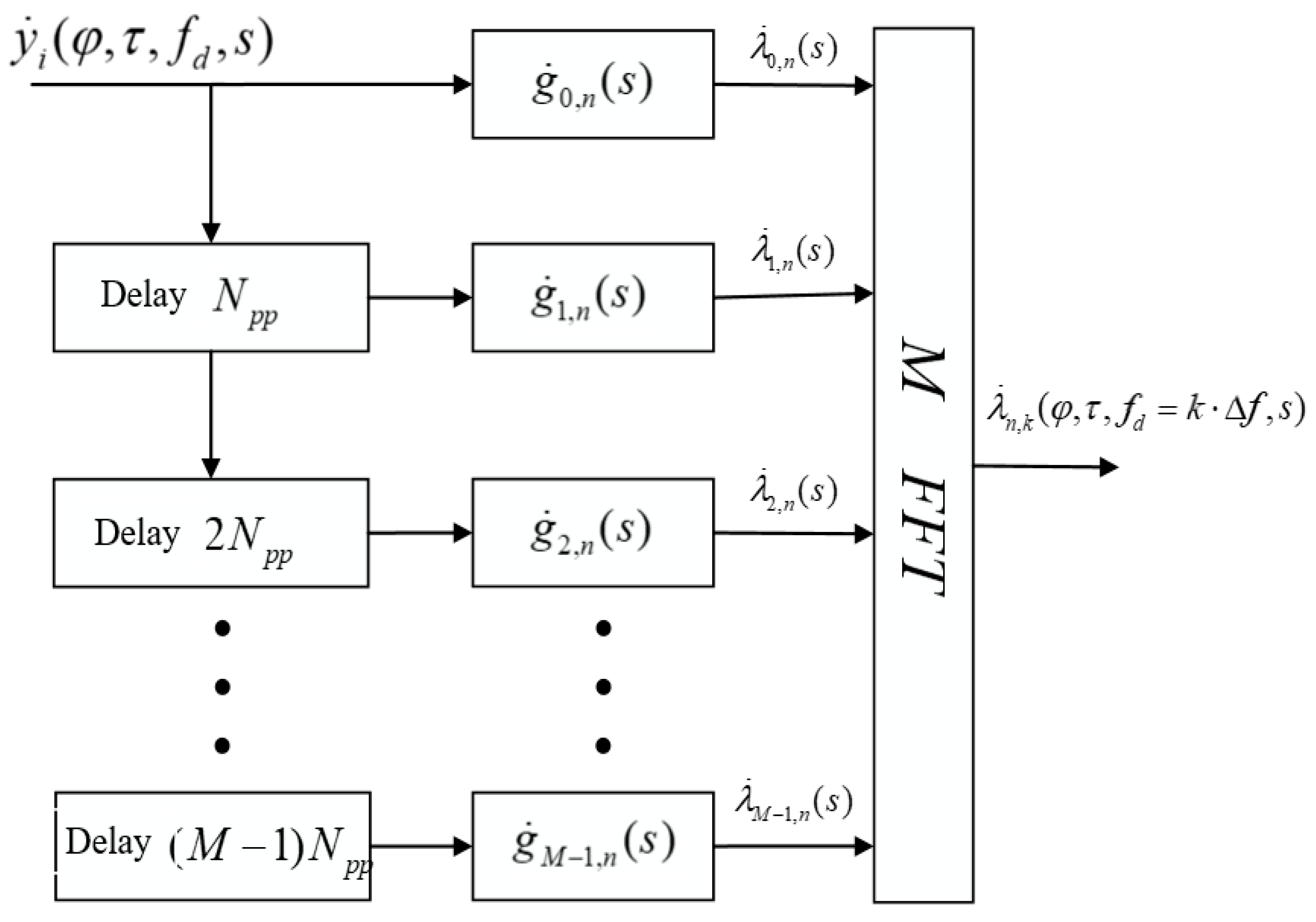
4.2. Algorithm with Doppler Estimation via FFT

Multiplication by complex exponents and the subsequent summation to further estimate the Doppler frequency shift can be done using the FFT.

Let $f_d=k\frac{f_s}{N}$, then Equation (10) can be represented as:

$${\dot{\lambda }}_{n,k}(f_d=k\cdot \Delta f,s)={\displaystyle \sum _{m=0}^{M-1}{\dot{\lambda }}_{m,n}(s)\cdot e^{j2\pi km}},$$

(13)

where

$$\begin{array}{l}{\dot{\lambda }}_{m,n}(s)={\displaystyle \sum _{l=0}^{N_{pp}-1}{\dot{y}}_{m,l}{\dot{g}}_{m,n-l}^{\ast }(s)},\\ n=0÷N_{pp}-1,m=0÷M-1.\end{array}$$

(14)

Equation (11) can be calculated using FFT algorithms from ${\dot{\lambda }}_{m,n}(s)$ for each $k$. This algorithm, in contrast to the algorithm with multiplications by complex exponents, makes it possible to estimate the Doppler frequency shift only for $f_d=k\cdot \Delta f$, where $k=[-\frac{N_{pp}}{2}:\frac{N_{pp}}{2}]$. The scheme of the filter matched with a series of sequences with searches for Doppler frequency shifts through the FFT is shown in Figure 4.

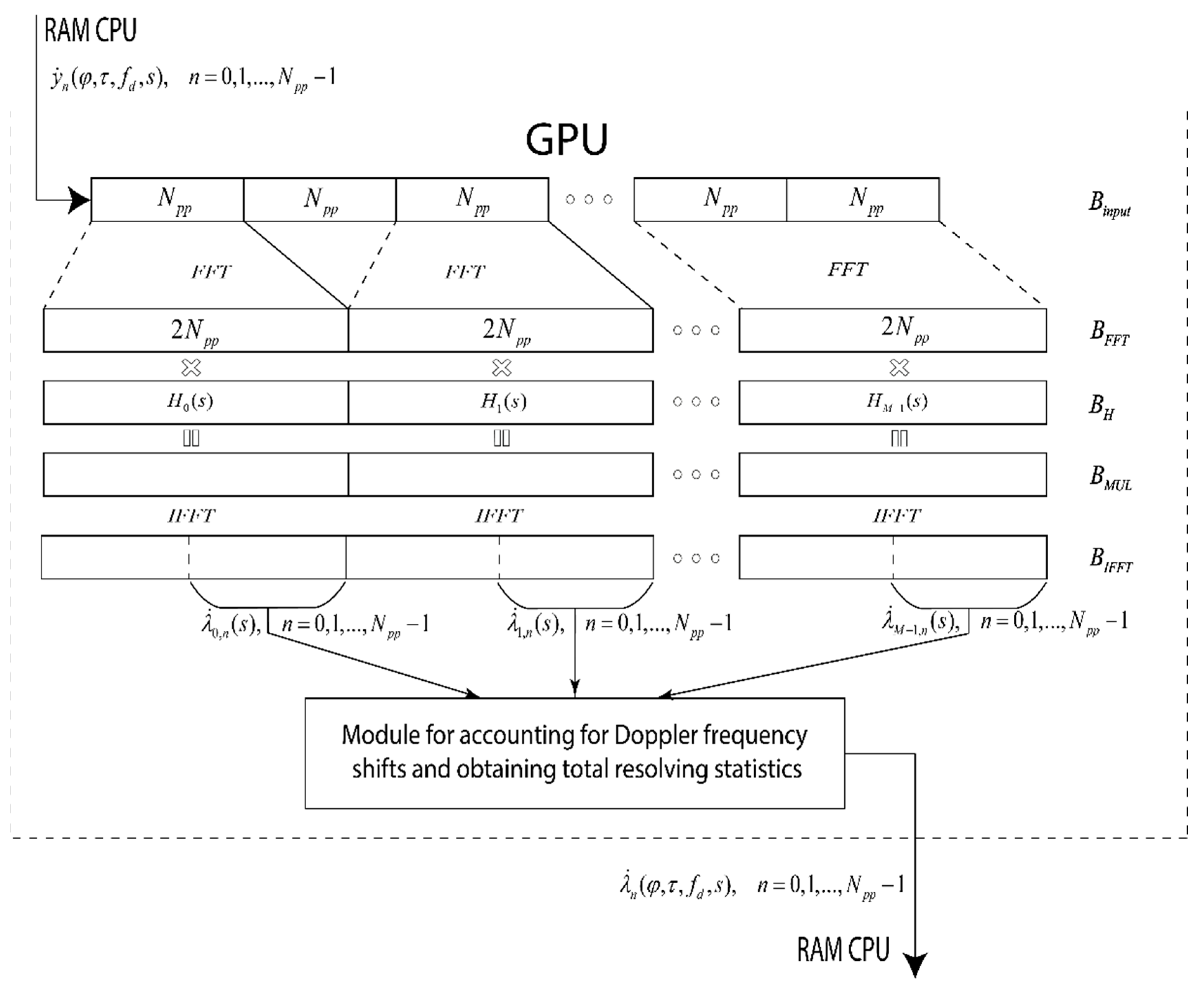
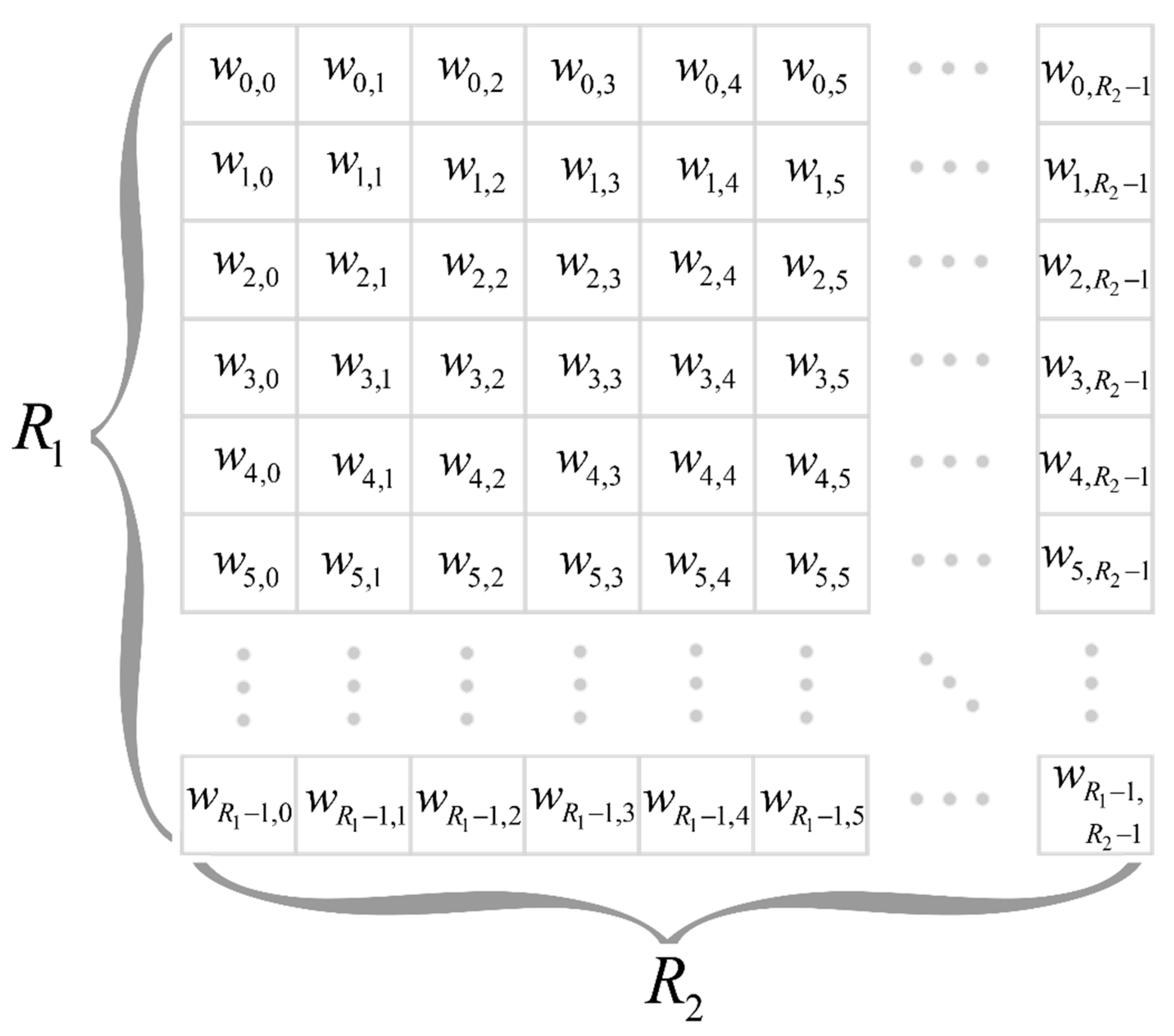
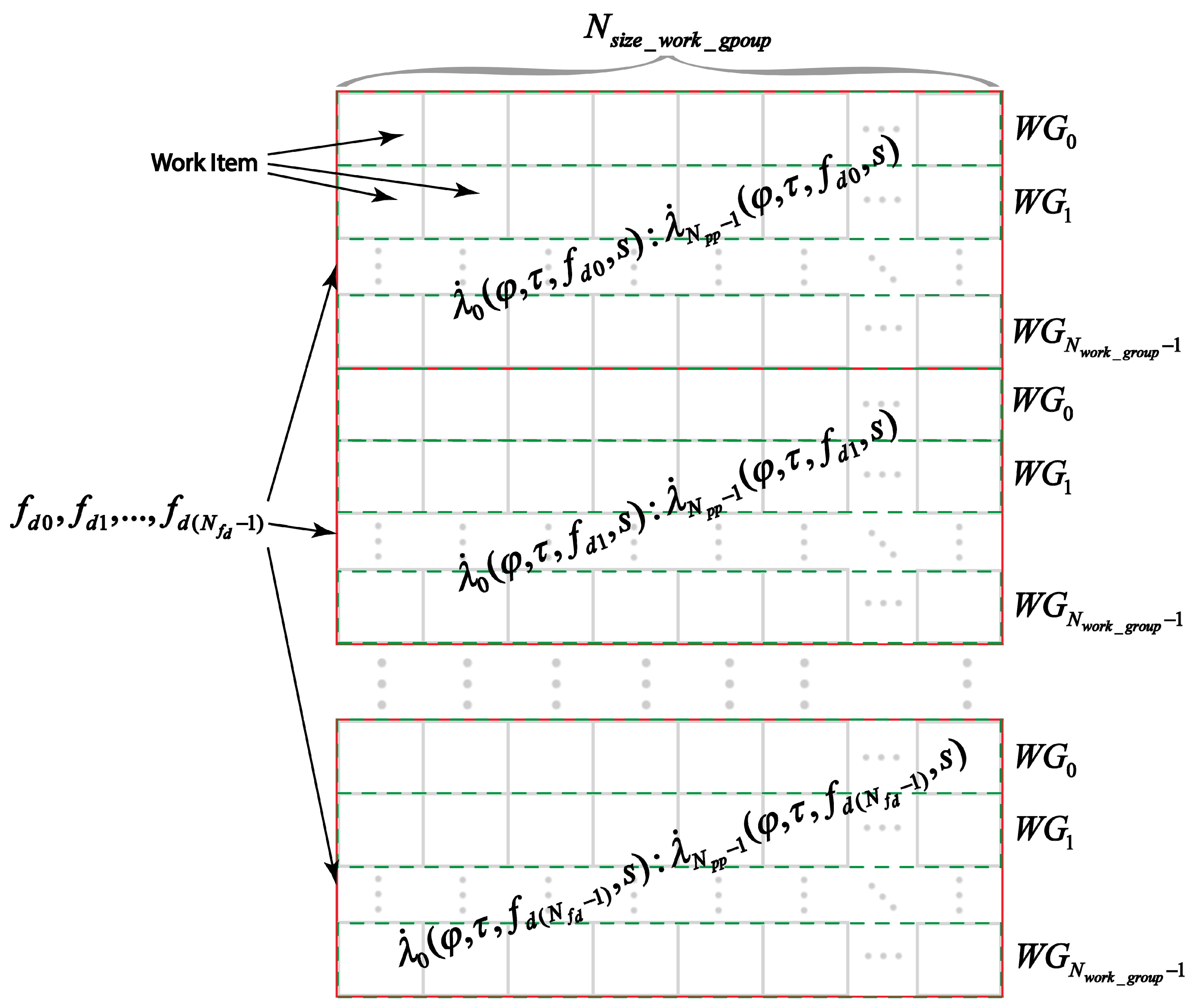
5. GPU Implementation

A matched filter with a series of sequences on the GPU is implemented using the fast convolution algorithm “Overlap and Save” [36] and the FFT and IFFT parallel computation library on the GPU–clFFT, implemented on OpenCL [37] (see Figure 5). The clFFT library is developed by clMathLibraries, an OpenCL library implementation of discrete fast Fourier transforms. The input data are loaded into the GPU in blocks of $N_{pp}$ samples. Loading is performed into a circular buffer $B_{input}$, size $N_{pp}(M+1)$. After loading the next block of samples, the buffer $B_{input}$ is fed to the calculation of the FFT with the size of $2N_{pp}$ with an overlap in $N_{pp}$ samples. FFT results are written to a buffer $B_{FFT}$, size $2N_{pp}M$. Post-FFT samples are multiplied with frequency response samples $\begin{array}{cc}{H}_i(s),& i=0,1,\dots ,M-1\end{array}$. The multiplication result is written to the buffer $B_{MUL}$ and fed to the calculation of the IFFT, size $2N_{pp}$. Samples after this IFFT are placed in the $B_{IFFT}$ buffer. The second half of each $2N_{pp}$ sample is the response of the filter ${\dot{\lambda }}_{m,n}(s)$ matched to the $m$-th sequence.

Received responses are transferred to the module for taking into account Doppler frequency shifts and obtaining the total decision statistics. This module is made in two versions. The first option is to directly multiply by complex exponents and then sum the filter responses. Multiplication operations by complex exponents are performed by calculating different samples of decision statistics using different GPU work items (WI).

The work items set $w_{i,j}$ of the graphic processor is represented as a matrix $W$, dimension $R_1\times R_2$ (see Figure 6). Where $R_1$ and $R_2$ are numbers of work items in the 1st and 2nd dimension, respectively. These values determined by GPU implementation and have to be taken into account in the parallelization of the algorithm adaptation for GPU.

Within the available number of work items, it is proposed to parallelize the calculation of all samples of the decision statistics for all possible values of the Doppler frequency shifts $f_d$. The required number of work items to compute decision statistic samples ${\dot{\lambda }}_n(f_d,s)$ for a single Doppler frequency shift value is $N_{pp}$. The maximum number of work items per calculation of the decision statistic samples for one value of the Doppler frequency shift can be calculated as:

$$N_{\max \_items\_\exp }=\lfloor \frac{R_1{R}_2}{N_{f_d}}\rfloor .$$

(15)

Then, the actual number of work items is defined as:

$$N_{items\_\exp }=\min (N_{\max \_items\_\exp },N_{pp}).$$

(16)

In the case when required number of work items exceeds number of available GPU items, some work items will calculate several samples of decision statistics ${\dot{\lambda }}_n(f_d,s)$.

When performing calculations on the GPU, work items are combined into work groups (WG). The best performance is achieved by setting the work group size $N_{size\_work\_group}$ to the maximum, which is determined by the specific GPU implementation. The number of work groups for computing decision statistics samples ${\dot{\lambda }}_n(f_d,s)$ for one value of Doppler frequency shift:

$$N_{work\_group}=\lceil \frac{N_{items\_\exp }}{N_{size\_work\_group}}\rceil .$$

(17)

The distribution of calculations between work items and GPU work groups is shown in Figure 7. This figure shows that the decision statistics values calculation ${\dot{\lambda }}_n(\phi ,\tau f_d,s)$ is divided into $N_{f_d}$ groups by $N_{work\_group}\times N_{size\_work\_group}$ work items. Each of these groups performs the calculation of the decision statistics samples ${\dot{\lambda }}_n(\phi ,\tau f_d,s)$ for one of the possible values of the Doppler frequency shift $f_d$. This improves the performance of the algorithm by performing parallel computations.

The second option for building a module for taking into account Doppler frequency shifts and obtaining the total decision statistics was performed using the FFT through the clFFT library. According to Equation (11) and Figure 4, the FFT must be taken from the $n$-th samples of all responses ${\dot{\lambda }}_{m,n}(s)$. The clFFT library allows you to perform all the necessary FFTs using a buffer $B_{IFFT}$ without additional memory operations. Figure 8 shows that the clFFT library allows you to perform an FFT from all $n$-th samples for all ${\dot{\lambda }}_{m,n}(s)$, $n=0÷N_{pp}-1,m=0÷M-1$ that were in the buffer $B_{IFFT}$ without additional data copies. The number of these FFT operations is $M$.

The FFT results are written to the buffer $B_{mf}$ in such a way that the decision statistics ${\dot{\lambda }}_n(f_d,s)$ for different values of the Doppler frequency shift are sequentially stored in the memory.

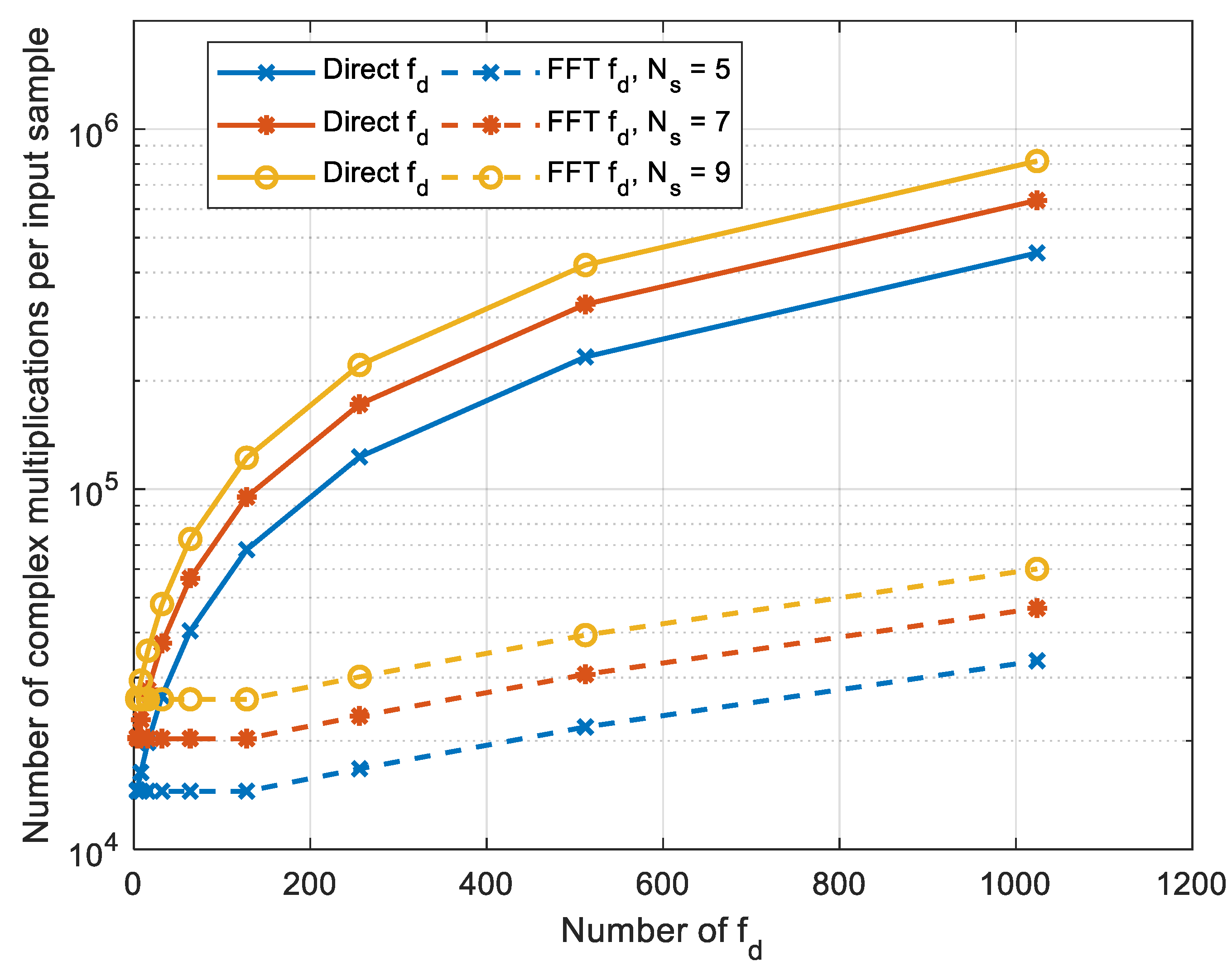
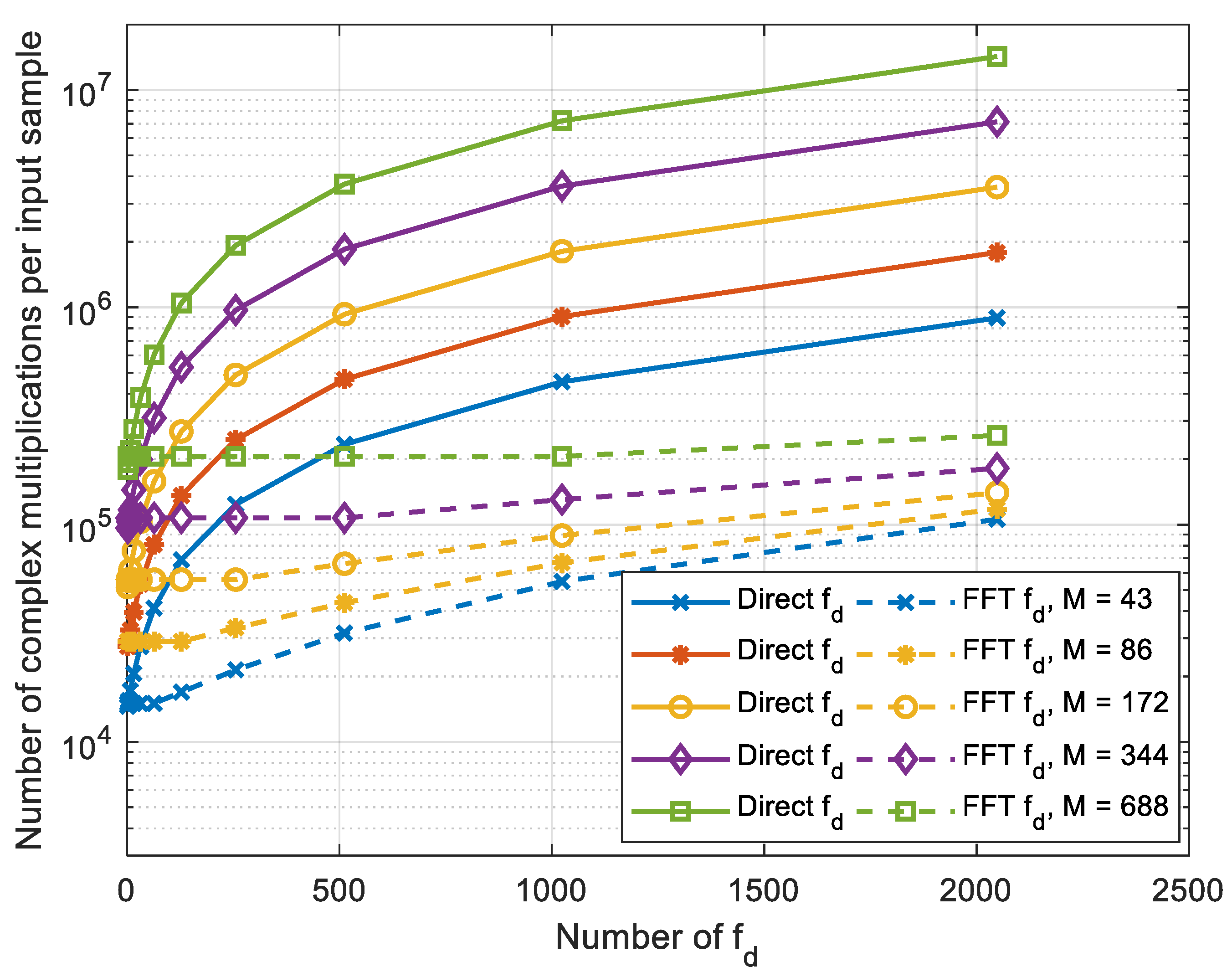
6. Comparison of Algorithms Computational Complexity

Computational complexity is affected by the number of possible values $f_d$ and $s$, which are defined as $N_s$ and $N_{f_d}$, respectively. Computational complexity is given in the number of complex multiplications per one input sample. Computational complexity of the device for joint detection and estimation of signal parameters for two implementations of the algorithm is defined as:

$$N_{cm}=\left(2M\left({\log }_2(2N_{pp})-1\right)+M{N}_{f_d}\right)N_s,$$

(18)

$$N_{cm\_fft}=\left(2M\left({\log }_2(2N_{pp})-1\right)+\frac{N_{f_d}}{2}\left({\log }_2(N_{f_d})-2\right)\right)N_s.$$

(19)

Thus, computational complexity of the proposed algorithm depends on the number of partitions of the original sequence $M$, the duration of one part of the original sequence $N_{pp}$, the number of possible values of Doppler shifts in frequency $N_{f_d}$, and slopes of the dispersion characteristic of the ionospheric channel $N_s$.

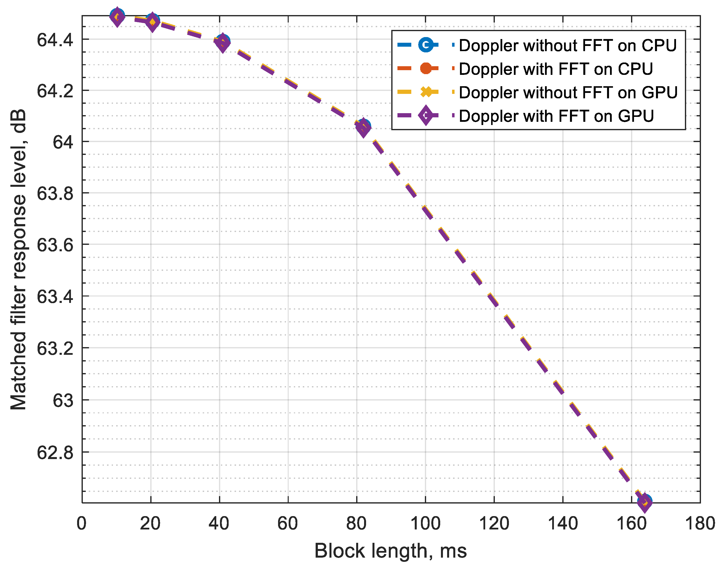
7. Test Results on CPU and GPU

For the experiment, a six-core Intel Core i7-8700 CPU with a clock frequency of 3.2 GHz and a Geforce RTX 3060 GPU with 3584 CUDA cores, a base clock frequency of 1.32 GHz, and a 192-bit memory bus were used. The experiment was run on a computing platform of 32 GB of RAM with a speed of 2400 MT/s. The experiment was carried out in the operating system Linux Ubuntu 20.04 with Nvidia GPU driver version 460.73.01. The used clFFT library version was 2.12.2. For algorithm implementation, compilation was used with a gcc 9.4.0 compiler with compiler flags set to o2. To execute calculations, five cores and 10 threads of Intel Core i7-8700 CPU were used. One core and two threads were left for the needs of the operating system. Testing was performed on a signal with a bandwidth $\Delta F=400 \mathrm{kHz}$ and a duration $T=7$ s. The base of this signal was 64.5 dB. These parameters were chosen based on the results of field experiments carried out on single-hop ionospheric paths up to 3000 km long. The search ranges for the Doppler frequency shift and the slope of the dispersion characteristic of the ionospheric channel were also selected based on the results of field experiments. Dependence of the computational complexity on the number of possible values of Doppler shifts in frequency $N_{f_d}$ for a different number of slopes of the dispersion characteristic of the ionospheric channel $N_s$ for $N_{pp}=32768$ and $M=86$ is shown in Figure 9.

This graph shows that an increase in the number of possible values $N_{f_d}$ leads to a slight increase in computational complexity compared to an increase in the number of possible values $N_s$. The dependence of the number of complex multiplications on the number of possible values $f_d$ for a different number of splits $M$ of the original signal at is shown in Figure 10.

The number of experiments performed to obtain averaged results was 1000. Increasing the number $M$ leads to an increase in computational complexity.

Table 1. Experimental running time of the algorithms per one input sample, with different block durations.

Algorithm Implementation Type	Block Length 10.24 ms µs	Block Length 20.48 ms µs	Block Length 40.96 ms µs	Block Length 81.92 ms µs	Block Length 163.84 ms µs
Doppler without FFT on CPU	251.1	124.4	62.59	31.3	15.91
Doppler with FFT on CPU	17.83	9.17	5.88	3.98	2.51
Doppler without FFT on GPU	7.36	4.21	2.49	1.61	1.19
Doppler with FFT on GPU	3.91	2.03	1.29	0.91	0.55

shows the dependence of the algorithm running time on the block duration for $\begin{array}{cc}{f}_d=-5:0.05:5& N_{f_d}=201\end{array}$.

Table 2. GPU RTX 3060 Performance Boost vs. CPU Intel Core i7-8700.

Algorithm Implementation Type	Block Length 10.24 ms	Block Length 20.48 ms	Block Length 40.96 ms	Block Length 81.92 ms	Block Length 163.84 ms
Doppler without FFT	34.12	29.55	25.14	19.44	13.37
Doppler with FFT	4.56	4.52	4.56	4.37	4.56

shows how many times RTX 3060 GPU is faster than base Intel i7-8700 processor. It can be seen that the performance gain of the RTX 3060 GPU in the algorithm without FFT decreases with increasing block duration, while in the algorithm with FFT, it remains constant.

The TDP of the RTX 3060 GPU is 170W, while the TDP of the Intel Core i7-8700 is 65W. Thus, the increase in power consumption when using the RTX 3060 GPU compared to the Intel Core i7-8700 CPU is 2.62 times, and the minimum performance increase is 4.37 times. Therefore, it is advisable to use a GPU, since the increase in performance exceeds the loss in power consumption.

Dependence of the response level of the matched filter on the block duration at the Doppler shift $f_d=3$ is shown in Figure 11.

Implementation with Doppler shift estimation via FFT on the GPU is the most efficient and allows for processing one sample in less than 2 µs with a loss of no more than 0.5 dB. With a block duration of less than 80 ms, the loss does not exceed 0.5 dB.

8. Conclusions

This paper proposes two implementations of the joint detection and estimation of the parameters of signals with dispersion distortions on the CPU and GPU. In the first method, the estimation of the Doppler frequency shift is performed in a direct way, by multiplying by complex exponents. In the second method, estimation of the Doppler frequency shift is performed through the FFT. All FFTs in the proposed implementations are performed through the “Overlap and Save” fast convolution algorithm. The computational complexity of the proposed implementations of joint detection and estimation of signal parameters is calculated. It is shown that the method based on the estimation of the Doppler frequency shift through the FFT is the most computationally efficient. Implementation of this method on the GPU allows for the joint detection and estimation of signal parameters in real time. It is shown how the duration of a block in a matched filter with a series of sequences affects the response level. Reducing the block duration results in a reduction in matched response level loss but results in an increase in computational complexity.

References

1. Jorgenson, M.B.; Johnson, R.W.; Nelson, R.W. An Extension of Wideband HF Capabilities. In Proceedings of the IEEE Military Communications Conference, San Diego, CA, USA, 18–20 November 2013; pp. 1202–1206. [Google Scholar]
2. Pijoan, J.L.; Altadill, D.; Torta, J.M.; Alsina-Pagès, R.M.; Marsal, S.; Badia, D. Remote Geophysical Observatory in Antarctica with HF Data Transmission: A Review. Remote Sens. 2014, 6, 7233–7259. [Google Scholar] [CrossRef] [Green Version]
3. Kandaurov, N.A. Signal-Code Constructs for Wideband HF Communication. In Proceedings of the 2019 Systems of Signal Synchronization, Generating and Processing in Telecommunications, Yaroslavl, Russia, 1–3 July 2019; p. 5. [Google Scholar] [CrossRef]
4. Laraway, S.A.; Loera, J.; Moradi, H.; Farhang-Boroujeny, B. Experimental Comparison of FB-MC-SS and DS-SS in HF Channels. In Proceedings of the MILCOM 2018 IEEE Military Communications Conference (MILCOM), Los Angeles, CA, USA, 29–31 October 2018; pp. 714–719. [Google Scholar] [CrossRef]
5. Deumal, M.; Vilella, C.; Socoro, J.; Alsina-Pagès, R.M.; Pijoan, J.L. A DS-SS signaling based system proposal for low SNR HF digital communications. In Proceedings of the 10th International Conference on Ionospheric Radio Systems and Techniques, London, UK, 18–21 July 2006; pp. 128–132. [Google Scholar]
6. Laraway, S.A.; Farhang-Boroujeny, B. Performance Analysis of a Multicarrier Spread Spectrum System in Doubly Dispersive Channels with Emphasis on HF Communications. IEEE Open J. Commun. Soc. 2020, 1, 462–476. [Google Scholar] [CrossRef]
7. Sun, H.; Yang, G.; Cui, X.; Zhu, P.; Jiang, C. Design of an Ultrawideband Ionosonde. IEEE Geosci. Remote Sens. Lett. 2015, 12, 1042–1045. [Google Scholar] [CrossRef]
8. Ivanov, D.V. Methods and Mathematical Models for Study of the Propagation of Decameter Complex Signals and Correction its Dispersion Distortions; MarSTU: Yoshkar-Ola, Russia, 2006. [Google Scholar]
9. Male, J.; Porte, J.; Gonzalez, T.; Maso, J.M.; Pijoan, J.L.; Badia, D. Analysis of the Ordinary and Extraordinary Ionospheric Modes for NVIS Digital Communications Channels. Sensors 2021, 21, 2210. [Google Scholar] [CrossRef] [PubMed]
10. Adjemov, S.S.; Lobov, E.M.; Kandaurov, N.A.; Lobova, E.O. Methods and algorithms of broadband HF signals dispersion distortion compensation. In Proceedings of the 2019 Systems of Signal Synchronization, Generating and Processing in Telecommunications (SYNCHROINFO), Yaroslavl, Russia, 1–3 July 2019; pp. 1–9. [Google Scholar] [CrossRef]
11. Barnes, R.I.; Earl, G.F. A wideband technique for micro-ranging in OTHR. In Proceedings of the 2008 IEEE Radar Conference, Rome, Italy, 26–30 May 2008; pp. 1–6. [Google Scholar] [CrossRef]
12. Huang, D.; Liu, E.; Hu, H.; Liu, J. Algorithm for the estimation of ionosphere parameters from ground scatter echoes of SuperDARN. Sci. China Technol. Sci. 2018, 61, 1755–1764. [Google Scholar] [CrossRef]
13. Ajemov, S.S.; Lobov, E.M.; Kandaurov, N.A.; Lobova, E.O.; Lipatkin, V.I. Algorithms of Estimating and Compensating the Dispersion Distortions of Wideband Signals in the HF Channel. H&ES Res. 2021, 13, 57–74. [Google Scholar]
14. Lipatkin, V.I.; Lobova, E.O.; Kandaurov, N.A. Wideband Signals Dispersion Distortions Optimum Tracking Compensator Based On Digital Filter Banks Using Farrow Filters. In Proceedings of the 2020 Systems of Signals Generating and Processing in the Field of on Board Communications, Moscow, Russia, 19–20 March 2020; p. 6. [Google Scholar] [CrossRef]
15. Lipatkin, V.I.; Lobova, E.O. Broadband Noise-like Signal Parameters Joint Estimation Quality with Dispersion Distortions in the Ionospheric Channel. In Proceedings of the 2020 Systems of Signal Synchronization, Generating and Processing in Telecommunications, SYNCHROINFO 2020, Svetlogorsk, Russia, 1–3 July 2020; p. 6. [Google Scholar] [CrossRef]
16. Lipatkin, V.I.; Lobova, E.O.; Telengator, K.E. The Influence of the Quality of the Estimation of Dispersion Distortions of a Broadband HF Signal on the Noise Immunity of a Radio Link. In Proceedings of the 2021 Systems of Signal Synchronization, Generating and Processing in Telecommunications, SYNCHROINFO 2021, Svetlogorsk, Russia, 30 June–2 July 2021; p. 4. [Google Scholar] [CrossRef]
17. Lipatkin, V.I.; Lobov, E.M.; Lobova, E.O.; Kandaurov, N.A. Cramer-Rao Bounds for Wideband Signal Parameters Joint Estimation in Ionospheric Frequency Dispersion Distortion Conditions. In Proceedings of the 2021 Systems of Signals Generating and Processing in the Field of on Board Communications, Moscow, Russia, 16–18 March 2021; p. 7. [Google Scholar] [CrossRef]
18. Arnold, E.; Rodriguez-Morales, F.; Paden, J.; Leuschen, C.; Keshmiri, S.; Yan, S.; Ewing, M.; Hale, R.; Mahmood, A.; Blevins, A.; et al. HF/VHF Radar Sounding of Ice from Manned and Unmanned Airborne Platforms. Geosciences 2018, 8, 182. [Google Scholar] [CrossRef] [Green Version]
19. Davey, S.J.; Fabrizio, G.A.; Rutten, M.G. Multipath-aware detection and tracking in skywave over-the-horizon radar. In Proceedings of the 2017 IEEE Radar Conference (RadarConf), Seattle, WS, USA, 8–12 May 2017; pp. 0636–0640. [Google Scholar] [CrossRef]
20. Fabrizio, G.; Zadoyanchuk, A.; Francis, D.; Nguyen, V. Using emitters of opportunity to enhance track geo-registration in HF over-the-horizon radar. In Proceedings of the 2016 IEEE Radar Conference (RadarConf), Philadelphia, PA, USA, 2–6 May 2016; pp. 1–5. [Google Scholar] [CrossRef]
21. Tao, S.; Ran, T.; Rong, S.R. A Fast Method for Time Delay, Doppler Shift and Doppler Rate Estimation. In Proceedings of the 2006 CIE International Conference on Radar, Shangai, China, 16–19 October 2006; pp. 1–4. [Google Scholar] [CrossRef]
22. Wang, Y.L.; Wu, Y.; Yi, S.C. An Efficient Direct Position Determination Algorithm Combined with Time Delay and Doppler. Circuits Syst. Signal Process 2016, 35, 635–649. [Google Scholar] [CrossRef]
23. Deng, L.; Wei, P.; Zhang, Z.; Zhang, H. Doppler Frequency Shift Based Source Localization in Presence of Sensor Location Errors. IEEE Access 2018, 6, 59752–59760. [Google Scholar] [CrossRef]
24. Ren, F.; Gao, H.; Yang, L. Distributed Multistatic Sky-Wave Over-The-Horizon Radar Based on the Doppler Frequency for MarineTarget Positioning. Electronics 2021, 10, 1472. [Google Scholar] [CrossRef]
25. Warrington, E.M.; Stocker, A.J. Measurements of the Doppler and multipath spread of the HF signals received over a path oriented along the midlatitude trough. Radio Sci. 2003, 38, 1–12. [Google Scholar] [CrossRef] [Green Version]
26. Knapp, C.H.; Karter, G.C. The Generalized Correlation Method for Estimation of Time Delay. IEEE Trans. Acoust. Speech Signal Process. 1976, 24, 320–327. [Google Scholar]
27. Stein, S. Algorithms for ambiguity function processing. IEEE Trans. Acoust. Speech Signal Process. 1981, 29, 588–599. [Google Scholar] [CrossRef]
28. Tolimieri, R.; Winograd, S. Computing the ambiguity surface. IEEE Trans. Acoust. Speech Signal Process. 1985, 33, 1239–1245. [Google Scholar] [CrossRef]
29. Zhihai, Z.; Tao, S. Research on Fast Computation of Ambiguity Function. In Proceedings of the 2008 Congress on Image and Signal Processing, Washington, DC, USA, 27–30 May 2008; pp. 188–192. [Google Scholar] [CrossRef]
30. Zhang, W.; Tao, R.; Ma, Y. Fast computation of the ambiguity function. In Proceedings of the 7th International Conference on Signal Processing, 2004, Beijing, China, 31 August–4 September 2004; Volume 3, pp. 2124–2127. [Google Scholar] [CrossRef]
31. Zhang, Z.; Wang, X.; Zou, Y.; Zhang, R. A Low Complexity Algorithm for Time-Frequency Joint Estimation of CAF Based on Numerical Fitting. In Proceedings of the 2020 IEEE/CIC International Conference on Communications in China (ICCC Workshops), Online, 9–11 August 2020; pp. 214–218. [Google Scholar] [CrossRef]
32. Ershov, R.A.; Morozov, O.A.; Fidelman, V.R. Time Delay Estimation of Ultra-wideband Signals by Calculation of the Cross-Ambiguity Function. In Wireless Communications, Networking and Applications. Lecture Notes in Electrical Engineering; Zeng, Q.A., Ed.; Springer: New Delhi, India, 2016; Volume 348. [Google Scholar]
33. Liu, G.; Yang, W.; Li, P.; Qin, G.; Cai, J.; Wang, Y.; Wang, S.; Yue, N.; Huang, D. MIMO Radar Parallel Simulation System Based on CPU/GPU Architecture. Sensors 2022, 22, 396. [Google Scholar] [CrossRef] [PubMed]
34. Kandaurov, N.A.; Lipatkin, V.I.; Varlamov, V.O. Implementing Digital Downconversion on a GPU. In Proceedings of the 2021 Systems of Signal Synchronization, Generating and Processing in Telecommunications, SYNCHROINFO 2021, Svetlogorsk, Russia, 30 June–2 July 2021; p. 8. [Google Scholar] [CrossRef]
35. He, Y.; Li, X.; Li, R.; Wang, J.; Jing, X. A Deep-Learning Method for Radar Micro-Doppler Spectrogram Restoration. Sensors 2020, 20, 5007. [Google Scholar] [CrossRef] [PubMed]
36. Proakis, J.G. Digital Communications, 4th ed.; McGraw-Hill: New York, NY, USA, 2001. [Google Scholar]
37. Munshi, A. The OpenCL Specification. Khronos OpenCL Working Group. Version 1.2. Document Revision 19. 2012. Available online: https://www.khronos.org/registry/OpenCL/specs/opencl-1.2.pdf (accessed on 17 April 2022).
Figure 1. Reference signal divided into M parts.
Sensors 22 03105 g001
Figure 2. Matched filter with a series of sequences with complex exponents.
Sensors 22 03105 g002
Figure 3. Scheme of the device for joint detection and signal parameter estimation.
Sensors 22 03105 g003
Figure 4. Matched filter with a series of sequences with searches over Doppler frequency shifts via FFT.
Sensors 22 03105 g004
Figure 5. Implementation diagram of a matched filter with a series of sequences.
Sensors 22 03105 g005
Figure 6. A set of GPU work items.
Sensors 22 03105 g006
Figure 7. Distribution of computations between GPU work items.
Sensors 22 03105 g007
Figure 8. Scheme of the module for taking into account Doppler frequency shifts and obtaining the total decisive statistics, implemented through the FFT.
Sensors 22 03105 g008
Figure 9. Dependence of the number of complex multiplications on the number of possible values f d for a different number of possible values of the slope of the dispersion characteristic of the ionospheric channel N s , M = 86 , N p p = 32768 .
Sensors 22 03105 g009
Figure 10. Dependence of the number of complex multiplications on the number of possible values f d for a different number of splits M of the original signal at N s = 10 .
Sensors 22 03105 g010
Figure 11. Dependence of the response level of the matched filter on the duration of the block with a Doppler frequency shift f d = 3 .
Sensors 22 03105 g011