
Facial Motion Analysis beyond Emotional Expressions

 , , and
Abstract
:1. Introduction
- A new dataset specifically acquired for GFE in the context of sign languages providing their face landmarks and AUs.
- A thorough assessment of GCN for Grammatical Facial Expression Recognition (GFER) with two types of input features (facial landmarks and action units) and comparison of this technique over two different GFE datasets and also against classical CNN techniques.
- A comparison of the experimental results with human performance on the new dataset.
2. Related Work
3. Materials
3.1. Datasets
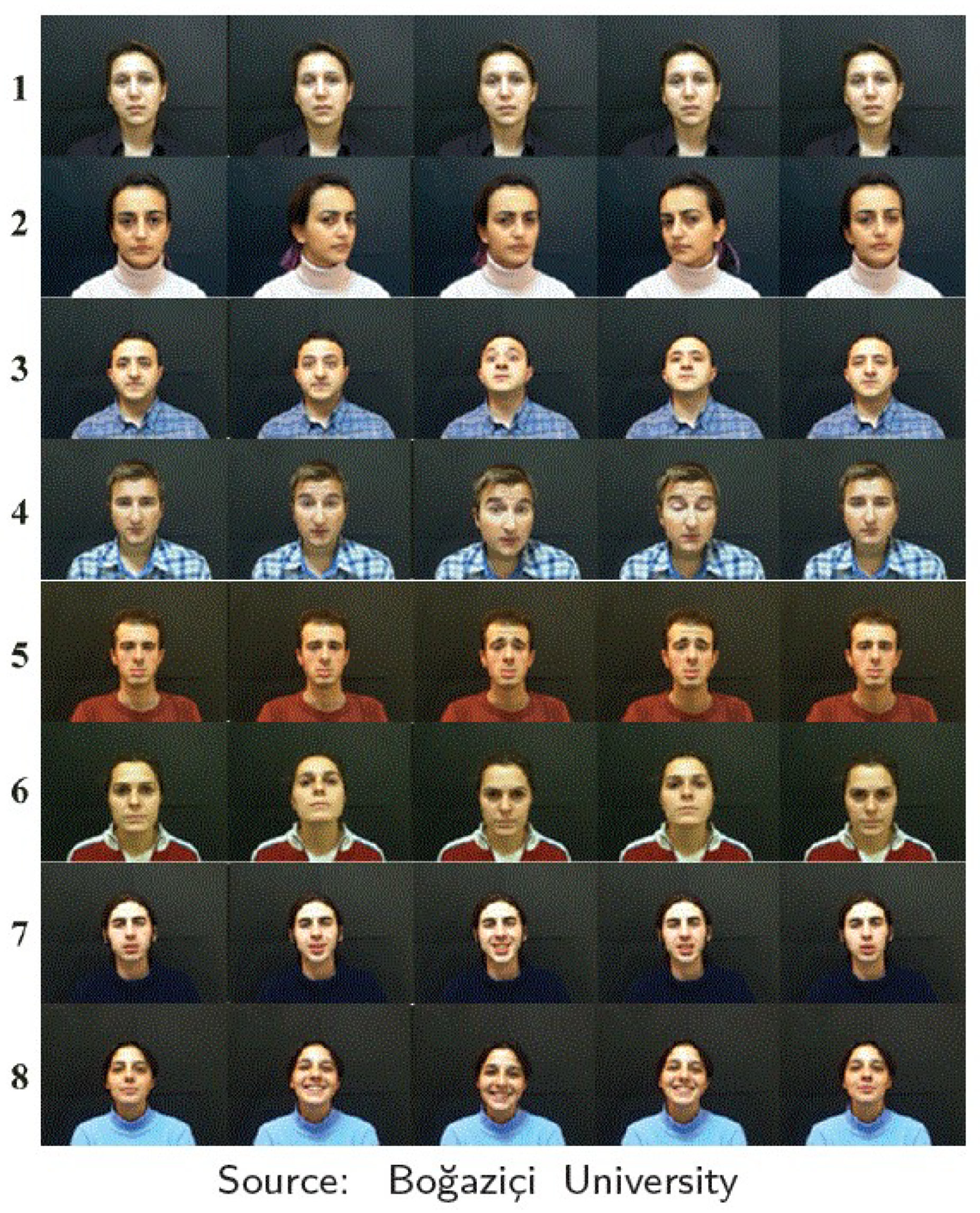
3.1.1. BUHMAP
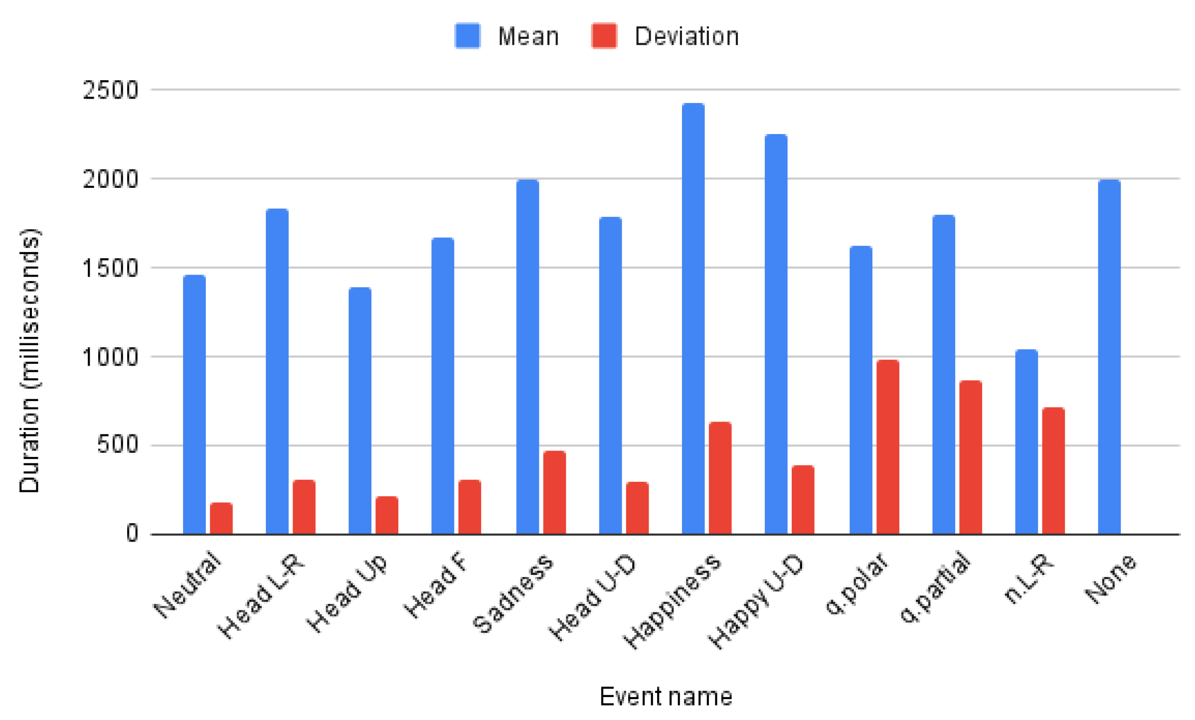
- Neutral: The neutral state of the face. The subject neither moves his/her face nor makes any facial expressions.
- Head L-R: Shaking the head to right and left sides. The initial side varies among subjects, and the shaking continues about 3–5 times. This sign is frequently used for negation in Turkish Sign Language (TSL).
- Head Up: Raise the head upwards while simultaneously raising the eyebrows. This sign is also frequently used for negation in TSL.
- Head F: Head is moved forward accompanied with raised eyebrows. This sign is frequently used to change the sentence to question form in TSL.
- Sadness: Lips turned down, eyebrows down. It is used to show sadness, e.g., when apologizing. Henceme subjects also move their head downwards.
- Head U-D: Nodding head up and down continuously. Frequently used for agreement.
- Happiness: Lips turned up. Subject smiles.
- Happy U-D: Head U-D + Happiness. The preceding two classes are performed together. It is introduced to be a challenge for the classifier in successfully distinguishing this confusing class with the two preceding ones.
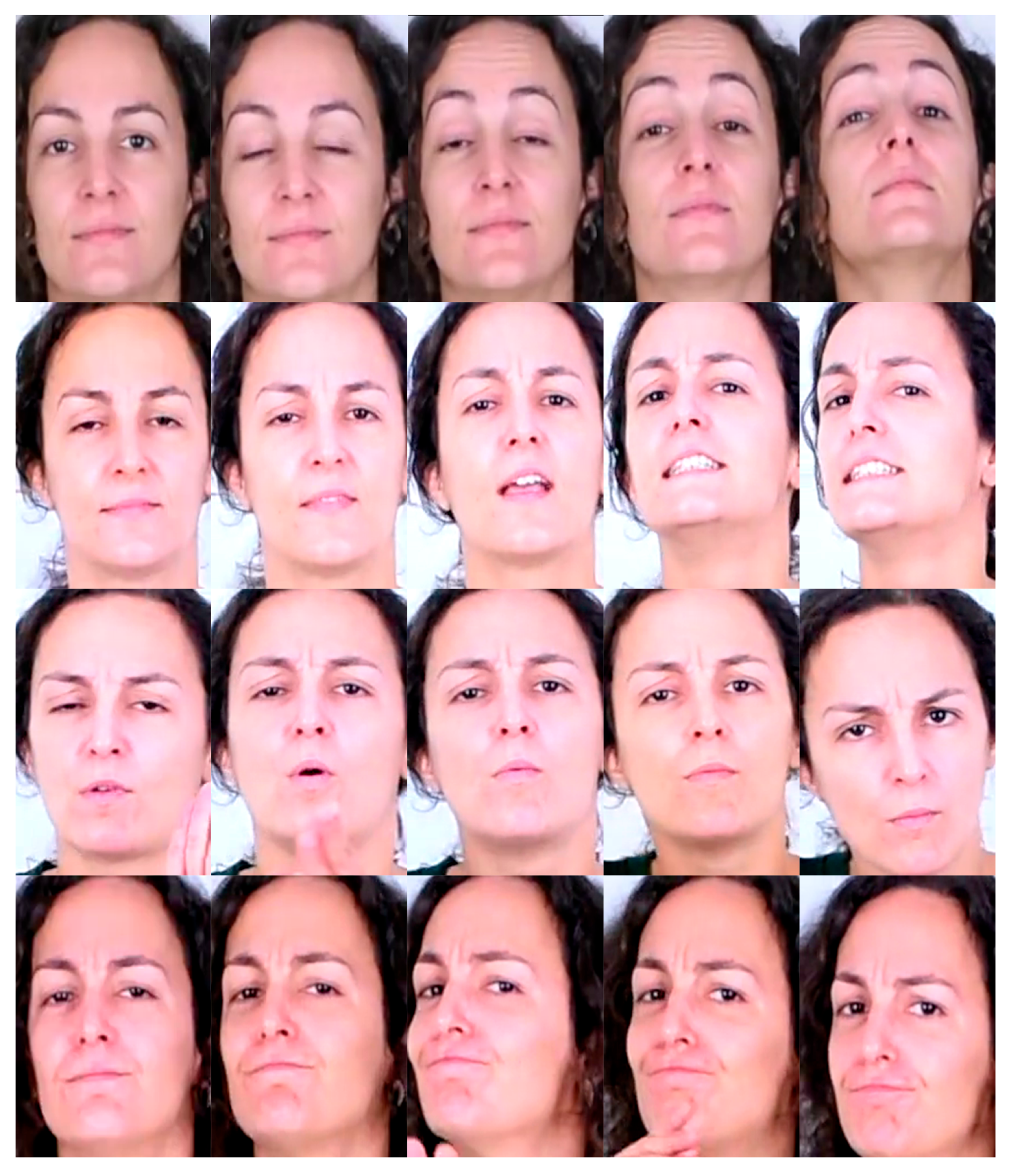
3.1.2. LSE_GFE
- q.polar: Yes/no question. Head and body is slightly moved forward accompanied with raising eyebrows. This sign is frequently used to change the sentence to close question form in LSE. 123 samples performed by 19 people.
- q.partial: Open question. Head and body is moved forward accompanied with frown eyebrows. This sign is frequently used to change the sentence to open question form in LSE. 265 samples performed by 13 people.
- q.other: General question form, not assimilable to polar (close) or partial (open). 16 samples from 9 people.
- n.L-R: Typical “no” negation, similar to Head L-R in BUHMAP. 176 samples performed by 22 people.
- n.other: General negation, not assimilable to n.L-R. 53 samples from 19 people.
- None: Samples without any of these questioning or negation components were extracted from the available videos of 24 people, to ensure the capacity of the model to detect the presence of non manual components. This class is quite different to the BUHMAP Neutral class, because in the LSE_GFE case, other communicative expressions can be included in the None class, i.e, dubitation with complex head and eyebrows movement.
3.2. Features
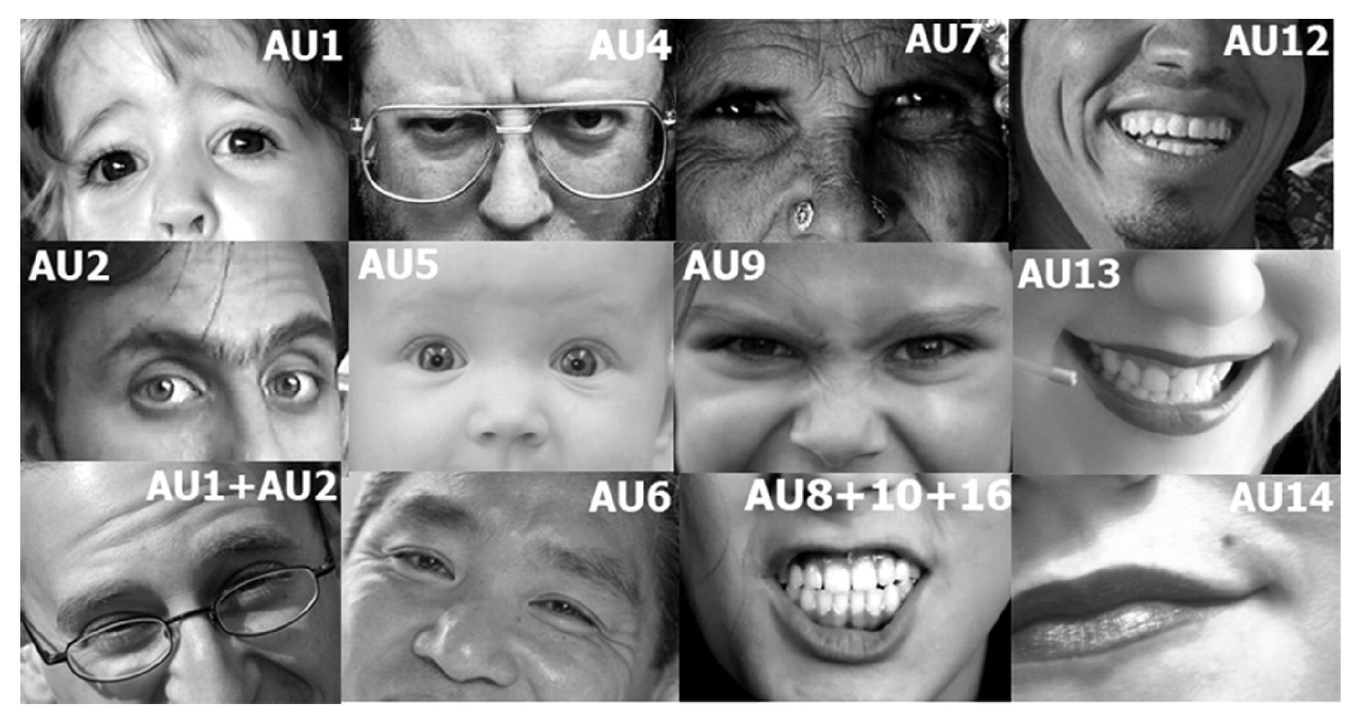
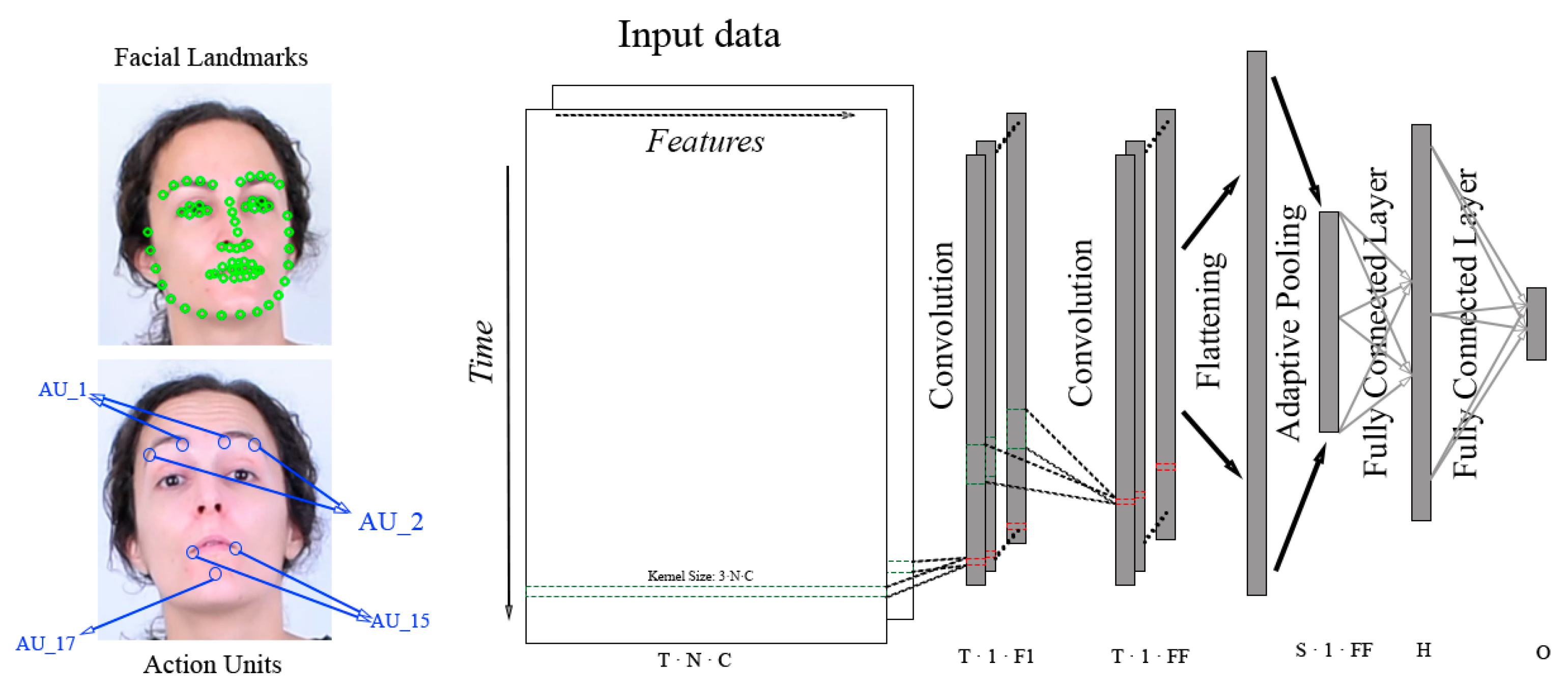
3.2.1. Action Units
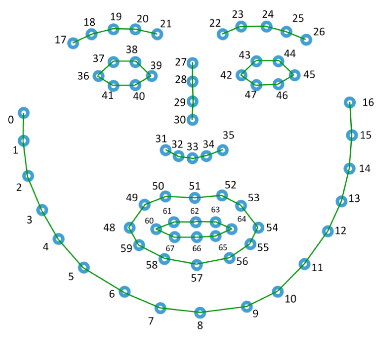
3.2.2. Facial Landmarks
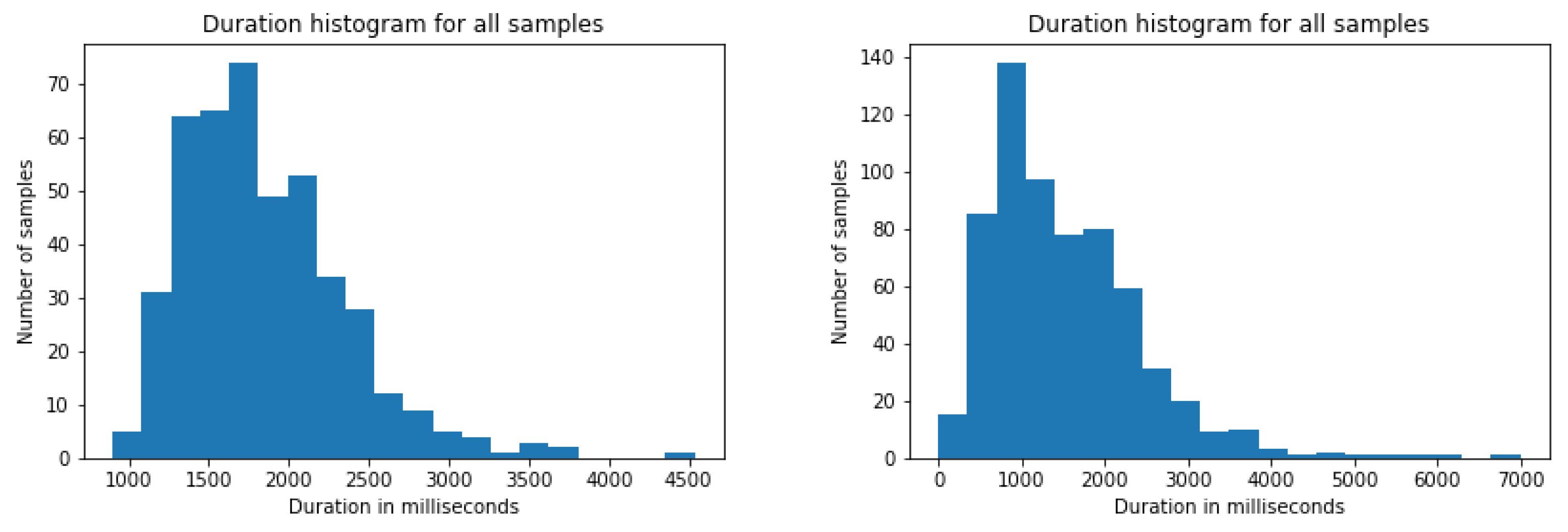
3.3. Video Sample Generation and Preprocessing
4. Methods
4.1. CNN Models
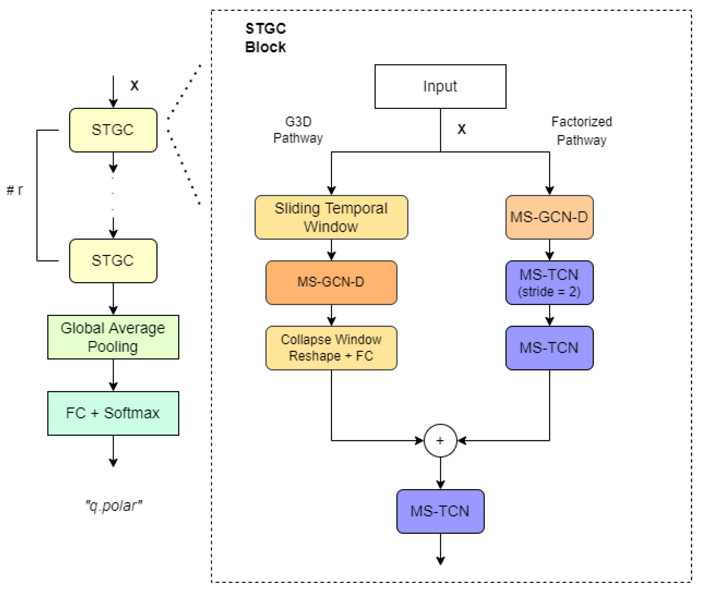
4.2. GCN Models
4.3. Evaluation Strategy and Metrics
5. Results
5.1. Ablation Study on MSG3D
- Use of data augmentation through horizontal flipping.
- The impact of graph topology.
- Number of spatial and temporal scales.
- The impact of GFE duration and frame-rate
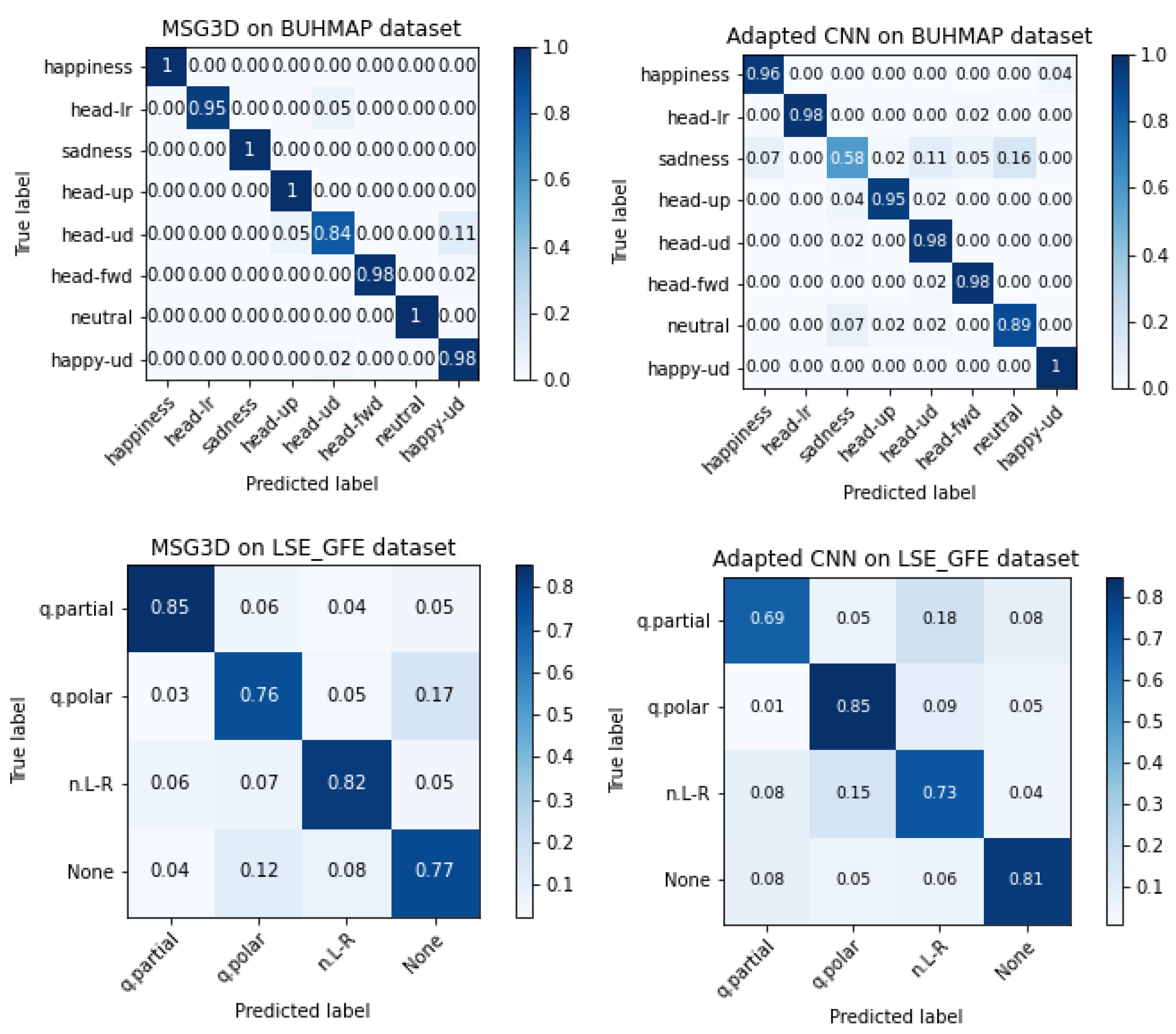
5.2. Accuracy Per Class
5.3. Comparison with State-of-the-Art Methods on BUHMAP
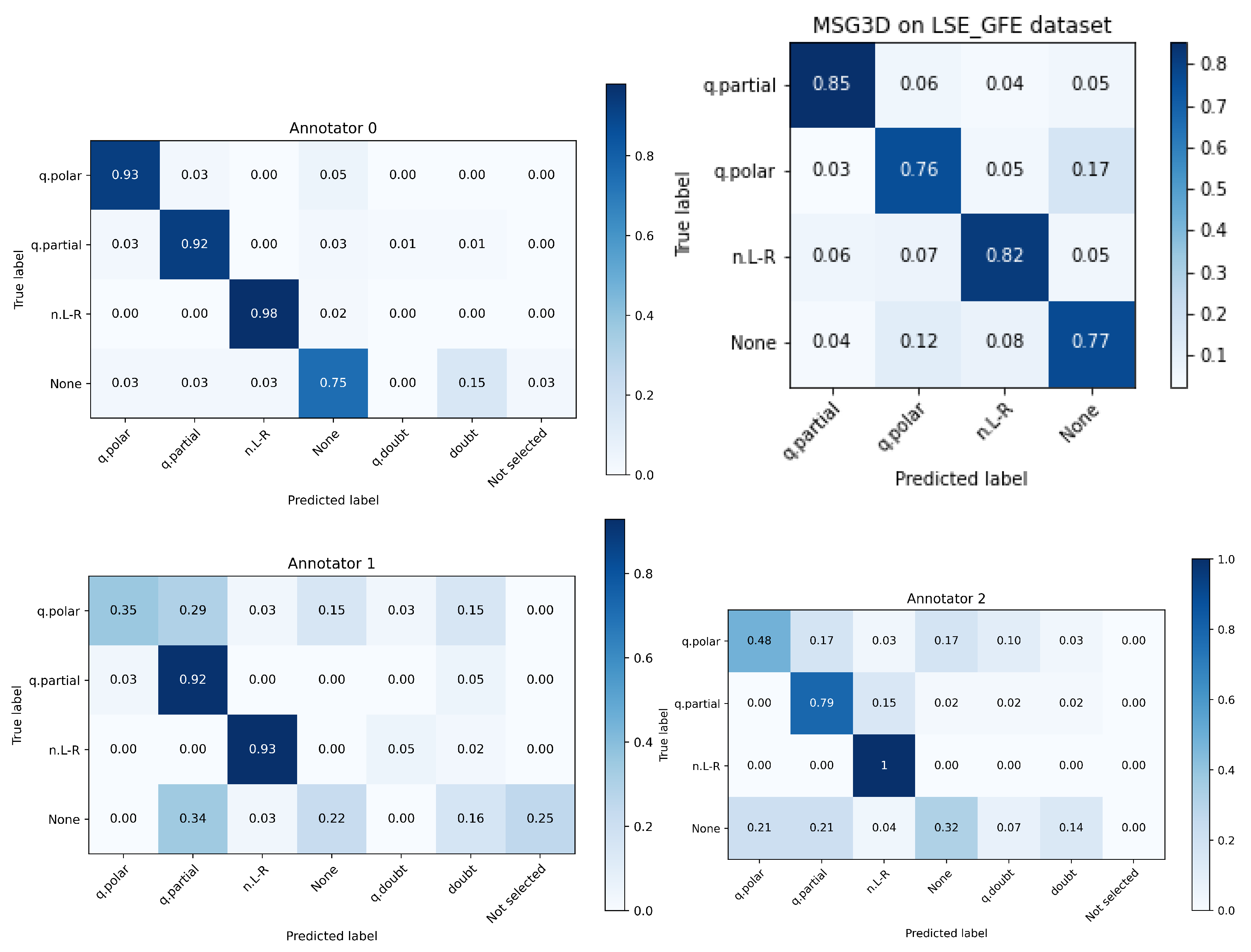
5.4. Comparison with Human Performance on LSE_GFE
- q.doubt -> “I am sure that it is question but I do not know whether it is polar or partial”,
- doubt -> “I am not sure whether it is a question or a negation but I am sure it is one of them”,
- not selected -> “I am not sure of any option. Pass”.
- Annotator 0 performs much better than the others, so it is clear that there’s an influence on having seen the footage and being involved in the acquisition process and discussions on the experiments.
- The class None, that was randomly extracted from interview segments where none of the 3 classes were present, is, by a large margin, the class with worse human performance. Even the annotator 0 performed worse than the automated system. This is a clear cue that the larger performance of annotator 0 was boosted by the previous knowledge of the dataset.
- The three annotators outperformed the automated system in classes q.partial and n.L-R, but two of them performed much worse in class q.polar where they showed many doubts.
6. Conclusions
Author Contributions
Funding
Informed Consent Statement
Data Availability Statement
Acknowledgments
Conflicts of Interest
References
- Ekman, P.; Friesen, W.V. Constants across cultures in the face and emotion. J. Personal. Hencec. Psychol. 1971, 17, 124. [Google Scholar] [CrossRef] [PubMed] [Green Version]
- McCullough, S.; Emmorey, K.; Sereno, M. Neural organization for recognition of grammatical and emotional facial expressions in deaf ASL signers and hearing nonsigners. Cogn. Brain Res. 2005, 22, 193–203. [Google Scholar] [CrossRef] [PubMed]
- Da Silva, E.P.; Costa, P.D.P.; Kumada, K.M.O.; De Martino, J.M.; Florentino, G.A. Recognition of Affective and Grammatical Facial Expressions: A Study for Brazilian Sign Language. In Proceedings of the Computer Vision—ECCV 2020 Workshops, Glasgow, UK, 23–28 August 2020; Bartoli, A., Fusiello, A., Eds.; Springer International Publishing: Cham, Switzerland, 2020; pp. 218–236. [Google Scholar]
- Li, S.; Deng, W. Deep facial expression recognition: A survey. IEEE Trans. Affect. Comput. 2020. [Google Scholar] [CrossRef] [Green Version]
- Ouellet, S. Real-time emotion recognition for gaming using deep convolutional network features. arXiv 2014, arXiv:1408.3750. [Google Scholar]
- Khor, H.Q.; See, J.; Phan, R.C.W.; Lin, W. Enriched long-term recurrent convolutional network for facial micro-expression recognition. In Proceedings of the 2018 13th IEEE International Conference on Automatic Face & Gesture Recognition (FG 2018), Xi’an, China, 15–19 May 2018; pp. 667–674. [Google Scholar]
- Ekman, P.; Friesen, W. Facial Action Coding System: A Technique for the Measurement of Facial Movement; Consulting Psychologists Press: Palo Alto, CA, USA, 1978. [Google Scholar]
- Zeng, Z.; Pantic, M.; Roisman, G.; Huang, T. A Survey of Affect Recognition Methods: Audio Visual and Spontaneous Expressions. IEEE Trans. Pattern Anal. Mach. Intell. 2009, 31, 39–58. [Google Scholar] [CrossRef] [PubMed]
- Valstar, M.; Gratch, J.; Schuller, B.; Ringeval, F.; Cowie, R.; Pantic, M. AVEC 2016-Depression, Mood, and Emotion Recognition Workshop and Challenge. In Proceedings of the 6th International Workshop on Audio/Visual Emotion Challenge, Amsterdam, The Netherlands, 16 October 2016; pp. 1483–1484. [Google Scholar] [CrossRef] [Green Version]
- Lien, J.J.; Kanade, T.; Cohn, J.F.; Li, C.C. Automated facial expression recognition based on FACS action units. In Proceedings of the Third IEEE International Conference on Automatic Face and Gesture Recognition, Nara, Japan, 14–16 April 1998; pp. 390–395. [Google Scholar]
- Devries, T.; Biswaranjan, K.; Taylor, G.W. Multi-task Learning of Facial Landmarks and Expression. In Proceedings of the 2014 Canadian Conference on Computer and Robot Vision, Montreal, QC, Canada, 6–9 May 2014; pp. 98–103. [Google Scholar] [CrossRef]
- Liu, X.; Cheng, X.; Lee, K. GA-SVM-Based Facial Emotion Recognition Using Facial Geometric Features. IEEE Sens. J. 2021, 21, 11532–11542. [Google Scholar] [CrossRef]
- Qiu, Y.; Wan, Y. Facial Expression Recognition based on Landmarks. In Proceedings of the 2019 IEEE 4th Advanced Information Technology, Electronic and Automation Control Conference (IAEAC), Chengdu, China, 20–22 December 2019; Volume 1, pp. 1356–1360. [Google Scholar] [CrossRef]
- Yan, J.; Zheng, W.; Cui, Z.; Tang, C.; Zhang, T.; Zong, Y. Multi-cue fusion for emotion recognition in the wild. Neurocomputing 2018, 309, 27–35. [Google Scholar] [CrossRef]
- Ahmad, T.; Jin, L.; Zhang, X.; Lai, S.; Tang, G.; Lin, L. Graph Convolutional Neural Network for Human Action Recognition: A Comprehensive Survey. IEEE Trans. Artif. Intell. 2021, 2, 128–145. [Google Scholar] [CrossRef]
- Ngoc, Q.T.; Lee, S.; Song, B.C. Facial landmark-based emotion recognition via directed graph neural network. Electronics 2020, 9, 764. [Google Scholar] [CrossRef]
- Liu, Y.; Zhang, X.; Lin, Y.; Wang, H. Facial Expression Recognition via Deep Action Units Graph Network Based on Psychological Mechanism. IEEE Trans. Cogn. Dev. Syst. 2020, 12, 311–322. [Google Scholar] [CrossRef]
- Jung, H.; Lee, S.; Yim, J.; Park, S.; Kim, J. Joint Fine-Tuning in Deep Neural Networks for Facial Expression Recognition. In Proceedings of the 2015 IEEE International Conference on Computer Vision (ICCV), Santiago, Chile, 7–13 December 2015; pp. 2983–2991. [Google Scholar] [CrossRef]
- Yan, S.; Xiong, Y.; Lin, D. Spatial Temporal Graph Convolutional Networks for Skeleton-Based Action Recognition. In Proceedings of the Thirty-Second AAAI Conference on Artificial Intelligence and Thirtieth Innovative Applications of Artificial Intelligence Conference and Eighth AAAI Symposium on Educational Advances in Artificial Intelligence, New Orleans, LO, USA, 2–7 February 2018. [Google Scholar]
- Heidari, N.; Iosifidis, A. Progressive Spatio–Temporal Bilinear Network with Monte Carlo Dropout for Landmark-based Facial Expression Recognition with Uncertainty Estimation. In Proceedings of the 23rd International Workshop on Multimedia Signal Processing, MMSP 2021, Tampere, Finland, 6–8 October 2021; pp. 1–6. [Google Scholar] [CrossRef]
- Lucey, P.; Cohn, J.F.; Kanade, T.; Saragih, J.; Ambadar, Z.; Matthews, I. The Extended Cohn-Kanade Dataset (CK+): A complete dataset for action unit and emotion-specified expression. In Proceedings of the 2010 IEEE Computer Society Conference on Computer Vision and Pattern Recognition workshops, San Francisco, CA, USA, 13–18 June 2010; pp. 94–101. [Google Scholar] [CrossRef] [Green Version]
- Zhao, G.; Huang, X.; Taini, M.; Li, S.Z.; Pietikäinen, M. Facial expression recognition from near-infrared videos. Image Vis. Comput. 2011, 29, 607–619. [Google Scholar] [CrossRef]
- Valstar, M.F.; Pantic, M. Induced disgust, happiness and surprise: An addition to the mmi facial expression database. In Proceedings of the 3rd International Workshop on EMOTION (Satellite of LREC): Corpora for Research on Emotion and Affect, Valetta, Malta, 23 May 2010; pp. 65–70. [Google Scholar]
- Dhall, A.; Goecke, R.; Lucey, S.; Gedeon, T. Collecting Large, Richly Annotated Facial-Expression Databases from Movies. IEEE Multimed. 2012, 19, 34–41. [Google Scholar] [CrossRef] [Green Version]
- Aifanti, N.; Papachristou, C.; Delopoulos, A. The MUG facial expression database. In Proceedings of the 11th International Workshop on Image Analysis for Multimedia Interactive Services WIAMIS 10, Desenzano del Garda, Italy, 12–14 April 2010; pp. 1–4. [Google Scholar]
- Yin, L.; Wei, X.; Sun, Y.; Wang, J.; Rosato, M. A 3D facial expression database for facial behavior research. In Proceedings of the 7th International Conference on Automatic Face and Gesture Recognition (FGR06), Southampton, UK, 10–12 April 2006; pp. 211–216. [Google Scholar] [CrossRef] [Green Version]
- Gunes, H.; Piccardi, M. A Bimodal Face and Body Gesture Database for Automatic Analysis of Human Nonverbal Affective Behavior. In Proceedings of the 18th International Conference on Pattern Recognition (ICPR’06), Hong Kong, China, 20–24 August 2006; Volume 1, pp. 1148–1153. [Google Scholar] [CrossRef] [Green Version]
- Aran, O.; Ari, I.; Guvensan, A.; Haberdar, H.; Kurt, Z.; Turkmen, I.; Uyar, A.; Akarun, L. A Database of Non-Manual Signs in Turkish Sign Language. In Proceedings of the 2007 IEEE 15th Signal Processing and Communications Applications, Eskisehir, Turkey, 11–13 June 2007; pp. 1–4. [Google Scholar] [CrossRef]
- Freitas, F.D.A. Grammatical Facial Expressions; UCI Machine Learning Repository: Irvine, CA, USA, 2014. [Google Scholar]
- Jiang, X.; Zong, Y.; Zheng, W.; Tang, C.; Xia, W.; Lu, C.; Liu, J. DFEW: A Large-Scale Database for Recognizing Dynamic Facial Expressions in the Wild. In Proceedings of the 28th ACM International Conference on Multimedia, Seattle, WA, USA, 12–16 October 2020; pp. 2881–2889. [Google Scholar]
- Sheerman-Chase, T.; Ong, E.J.; Bowden, R. Cultural factors in the regression of non-verbal communication perception. In Proceedings of the 2011 IEEE International Conference on Computer Vision Workshops (ICCV Workshops), Barcelona, Spain, 6–13 November 2011; pp. 1242–1249. [Google Scholar] [CrossRef] [Green Version]
- Silva, E.P.d.; Costa, P.D.P.; Kumada, K.M.O.; De Martino, J.M. SILFA: Sign Language Facial Action Database for the Development of Assistive Technologies for the Deaf. In Proceedings of the 2020 15th IEEE International Conference on Automatic Face and Gesture Recognition (FG 2020), Buenos Aires, Argentina, 16–20 November 2020; pp. 688–692. [Google Scholar] [CrossRef]
- Docío-Fernández, L.; Alba-Castro, J.L.; Torres-Guijarro, S.; Rodríguez-Banga, E.; Rey-Area, M.; Pérez-Pérez, A.; Rico-Alonso, S.; García-Mateo, C. LSE_UVIGO: A Multi-source Database for Spanish Sign Language Recognition. In Proceedings of the LREC2020 9th Workshop on the Representation and Processing of Sign Languages: Sign Language Resources in the Service of the Language Community, Technological Challenges and Application Perspectives, Marseille, France, 11–16 May 2020; pp. 45–52. [Google Scholar]
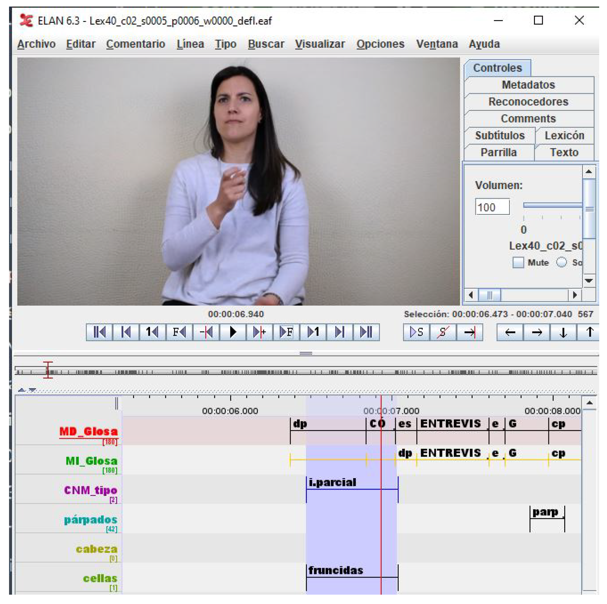
- Max Planck Institute for Psycholinguistics. The Language Archive [Computer Software]. Available online: https://archive.mpi.nl/tla/elan (accessed on 20 November 2020).
- Baltrušaitis, T.; Mahmoud, M.; Robinson, P. Cross-dataset learning and person-specific normalisation for automatic action unit detection. In Proceedings of the 2015 11th IEEE International Conference and Workshops on Automatic Face and Gesture Recognition (FG), Ljubljana, Slovenia, 4–8 May 2015; Volume 6, pp. 1–6. [Google Scholar]
- Zadeh, A.; Lim, Y.C.; Baltrušaitis, T.; Morency, L.P. Convolutional experts constrained local model for 3D facial landmark detection. In Proceedings of the 2017 IEEE International Conference on Computer Vision Workshops, Venice, Italy, 22–29 October 2017; pp. 2519–2528. [Google Scholar]
- Sandler, M.; Howard, A.; Zhu, M.; Zhmoginov, A.; Chen, L.C. MobileNetV2: Inverted Residuals and Linear Bottlenecks. arXiv 2019, arXiv:1801.04381. [Google Scholar]
- Liu, Z.; Zhang, H.; Chen, Z.; Wang, Z.; Ouyang, W. Disentangling and unifying graph convolutions for skeleton-based action recognition. In Proceedings of the IEEE Computer Society Conference on Computer Vision and Pattern Recognition, Seattle, WA, USA, 13–19 June 2020. [Google Scholar]
- Vázquez-Enríquez, M.; Alba-Castro, J.L.; Fernández, L.D.; Banga, E.R. Isolated Sign Language Recognition with Multi-Scale Spatial-Temporal Graph Convolutional Networks. In Proceedings of the 2021 IEEE/CVF Conference on Computer Vision and Pattern Recognition Workshops (CVPRW), Virtual, 19–25 June 2021; pp. 3457–3466. [Google Scholar]
- Li, M.; Chen, S.; Chen, X.; Zhang, Y.; Wang, Y.; Tian, Q. Actional-Structural Graph Convolutional Networks for Skeleton-based Action Recognition. arXiv 2019, arXiv:1904.12659. [Google Scholar]
- Aran, O.; Akarun, L. A multi-class classification strategy for Fisher scores: Application to signer independent sign language recognition. Pattern Recognit. 2010, 43, 1776–1788. [Google Scholar] [CrossRef] [Green Version]
- Çınar Akakın, H.; Sankur, B. Robust classification of face and head gestures in video. Image Vis. Comput. 2011, 29, 470–483. [Google Scholar] [CrossRef]
- Chouhayebi, H.; Riffi, J.; Mahraz, M.A.; Yahyaouy, A.; Tairi, H.; Alioua, N. Facial expression recognition based on geometric features. In Proceedings of the 2020 International Conference on Intelligent Systems and Computer Vision (ISCV), Fez, Morocco, 9–11 June 2020; pp. 1–6. [Google Scholar] [CrossRef]
- Ari, I.; Uyar, A.; Akarun, L. Facial feature tracking and expression recognition for sign language. In Proceedings of the 23rd International Symposium on Computer and Information Sciences, Istanbul, Turkey, 27–29 October 2008. [Google Scholar] [CrossRef]


| Primary Keywords | (“facial expression recognition” OR “facial emotion recognition” OR (“linguistic” OR “grammatical”) AND “facial expressions” AND “recognition”) OR (“facial micro-expression recognition”) AND (“video” OR “image sequences” OR “dynamic expressions” OR “temporary information” OR “temporal data” OR “spatial-temporal") |
| Secondary Keywords | (“action units” OR “landmarks”) |
| Last filtering | (“action units” OR “landmarks” AND “graph convolutional networks” |
| Name | Cites | Type of Expression | Acquisition Set Up | Classes | Videos | Persons |
|---|---|---|---|---|---|---|
| CK+ [21] | 1754 | emotions | controlled | 7 | 327 | 118 |
| OULU-CASIA [22] | 413 | emotions | controlled (light variation) | 6 | 480 | 80 |
| MMI [23] | 342 | induced emotions | natural | 6 | 213 | 30 |
| AFEW [24] | 316 | emotions | movies | 7 | 1426 | 330 |
| MUG [25] | 261 | induced emotions | semi-controlled | 6 | 1462 | 52 |
| BU-4DFE [26] | 154 | emotions | controlled | 6 | 606 | 101 |
| FABO [27] | 85 | induced emotions | semi-controlled | 9 | 1900 | 23 |
| BUHMAP [28] | 20 | sign-language/emotions | controlled | 8 | 440 | 11 |
| GFE-LIBRAS [29] | 10 | sign-language | natural | 9 | 36 | 2 |
| DFEW [30] | 8 | emotions | movies | 7 | 16,372 | - |
| LILiR [31] | 6 | non-verbal communication | natural | 4 | 527 | 2 |
| SILFA [32] | 3 | sign-language | semi-controlled | ? | 230 | 10 |
| Class | Female | Male |
|---|---|---|
| q.polar | 68 | 55 |
| q.partial | 174 | 91 |
| q.other | 10 | 6 |
| n.L-R | 105 | 71 |
| n.other | 29 | 24 |
| None | 109 | 99 |
| ID | q.polar | q.partial | n.L-R | None |
|---|---|---|---|---|
| p0003 | 19 | 47 | 20 | 13 |
| p0004 | 6 | 4 | 3 | 3 |
| p0006 | 15 | 49 | 20 | 34 |
| p0013 | 6 | 15 | 3 | 11 |
| p0025 | 6 | 14 | 4 | 11 |
| p0026 | 4 | 12 | 8 | 9 |
| p0028 | 5 | 18 | 3 | 11 |
| p0036 | 15 | 30 | 24 | 35 |
| p0037 | 7 | 18 | 9 | 34 |
| p0039 | 12 | 19 | 11 | 15 |
| p0041 | 6 | 13 | 8 | 16 |
| Model | Dataset | Feature | Weighted F1 | Accuracy | Parameters |
|---|---|---|---|---|---|
| MobilenetV2 | BUHMAP | landmarks | 2233768 | ||
| MobilenetV2 | BUHMAP | AUs | 2233480 | ||
| MobilenetV2 | LSE_GFE | landmarks | 2228344 | ||
| MobilenetV2 | LSE_GFE | AUs | 2228356 | ||
| VGG-11 | BUHMAP | landmarks | 128804040 | ||
| VGG-11 | BUHMAP | AUs | 128803464 | ||
| VGG-11 | LSE_GFE | landmarks | 128787652 | ||
| VGG-11 | LSE_GFE | AUs | 128787076 | ||
| custom CNN | BUHMAP | landmarks | 31992 | ||
| custom CNN | BUHMAP | AUs | 23912 | ||
| custom CNN | LSE_GFE | landmarks | 31732 | ||
| custom CNN | LSE_GFE | AUs | 23652 |
| Dataset | Feature | Weighted F1 | Accuracy | Parameters |
|---|---|---|---|---|
| BUHMAP | landmarks | 6527396 | ||
| BUHMAP | AUs | 2913570 | ||
| LSE_GFE | landmarks | 6525856 | ||
| LSE_GFE | AUs | 2912030 |
| Dataset | Flipping | Graph | Weighted F1 | Accuracy |
|---|---|---|---|---|
| BUHMAP | no | base | ||
| BUHMAP | yes | base | ||
| LSE_GFE | no | base | ||
| LSE_GFE | yes | base |
| Dataset | Graph | Weighted F1 | Accuracy |
|---|---|---|---|
| BUHMAP | base-graph | ||
| BUHMAP | empty-graph | ||
| LSE_GFE | base-graph | ||
| LSE_GFE | empty-graph |
| Dataset | Graph | (SS,TS) | Weighted F1 | Accuracy | Parameters |
|---|---|---|---|---|---|
| BUHMAP | base-graph | (8,8) | 6527396 | ||
| BUHMAP | base-graph | (1,1) | 2159676 | ||
| BUHMAP | empty-graph | (8,8) | 6527396 | ||
| BUHMAP | empty-graph | (1,1) | 2159676 | ||
| LSE_GFE | base-graph | (8,8) | 6525856 | ||
| LSE_GFE | base-graph | (1,1) | 2158136 | ||
| LSE_GFE | empty-graph | (8,8) | 6525856 | ||
| LSE_GFE | empty-graph | (1,1) | 2158136 |
| Dataset | Duration | FPS | Weighted F1 | Accuracy |
|---|---|---|---|---|
| BUHMAP | 4 s | 30 | ||
| BUHMAP | 4 s | 15 | ||
| BUHMAP | 2 s | 30 | ||
| BUHMAP | 2 s | 15 | ||
| LSE_GFE | 4 s | 30 | ||
| LSE_GFE | 4 s | 15 | ||
| LSE_GFE | 2 s | 50 | ||
| LSE_GFE | 2 s | 20 |
| System | Classes | Eval. Method | Accuracy | F1-Score |
|---|---|---|---|---|
| [41] | All | LOSO CV | ||
| [42] | 2 to 8 | LOSO CV | ||
| [43] | 1, 5 and 7 | Unknown | ||
| [44] | 2 a 8 | 1 person test | ||
| [44] | 2, 3, 4 and 7 | 1 person test | ||
| [44] | 2 a 8 | 5-fold CV | ||
| [44] | 2, 3, 4 and 7 | 5-fold CV | ||
| [44] | 2, 3, 4 and 7 | 2 persons test | ||
| Ours (best) | All | LOSO CV |
Publisher’s Note: MDPI stays neutral with regard to jurisdictional claims in published maps and institutional affiliations. |
© 2022 by the authors. Licensee MDPI, Basel, Switzerland. This article is an open access article distributed under the terms and conditions of the Creative Commons Attribution (CC BY) license (https://creativecommons.org/licenses/by/4.0/).
Share and Cite
Porta-Lorenzo, M.; Vázquez-Enríquez, M.; Pérez-Pérez, A.; Alba-Castro, J.L.; Docío-Fernández, L. Facial Motion Analysis beyond Emotional Expressions. Sensors 2022, 22, 3839. https://doi.org/10.3390/s22103839
Porta-Lorenzo M, Vázquez-Enríquez M, Pérez-Pérez A, Alba-Castro JL, Docío-Fernández L. Facial Motion Analysis beyond Emotional Expressions. Sensors. 2022; 22(10):3839. https://doi.org/10.3390/s22103839
Chicago/Turabian StylePorta-Lorenzo, Manuel, Manuel Vázquez-Enríquez, Ania Pérez-Pérez, José Luis Alba-Castro, and Laura Docío-Fernández. 2022. "Facial Motion Analysis beyond Emotional Expressions" Sensors 22, no. 10: 3839. https://doi.org/10.3390/s22103839
APA StylePorta-Lorenzo, M., Vázquez-Enríquez, M., Pérez-Pérez, A., Alba-Castro, J. L., & Docío-Fernández, L. (2022). Facial Motion Analysis beyond Emotional Expressions. Sensors, 22(10), 3839. https://doi.org/10.3390/s22103839