
Novel Downhole Electromagnetic Flowmeter for Oil-Water Two-Phase Flow in High-Water-Cut Oil-Producing Wells

Abstract
:1. Introduction
2. Theory of the Downhole Two-Electrode EMF
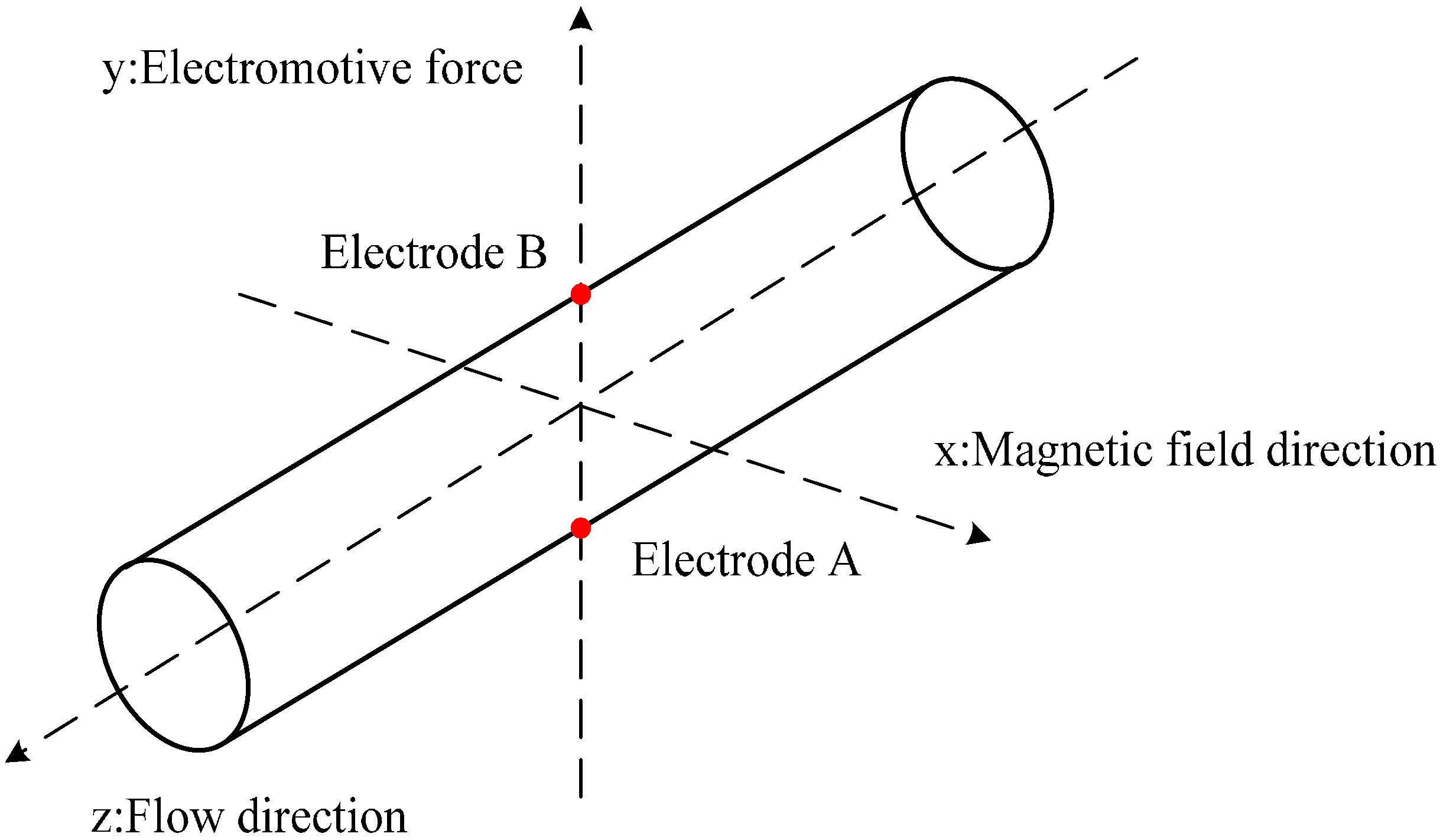
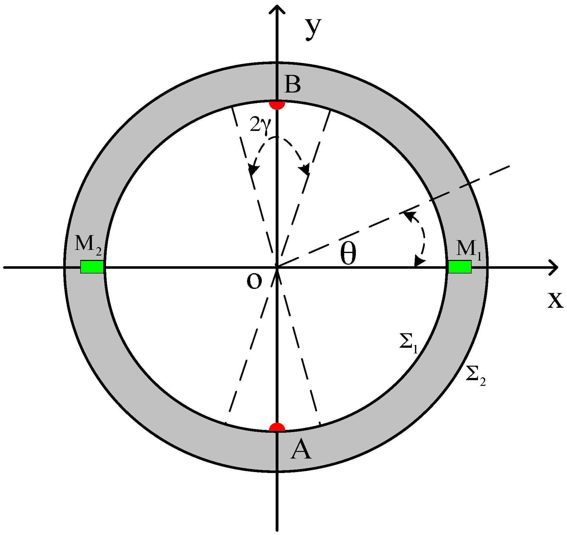
2.1. Ideal Response Model of the Two-Electrode EMF
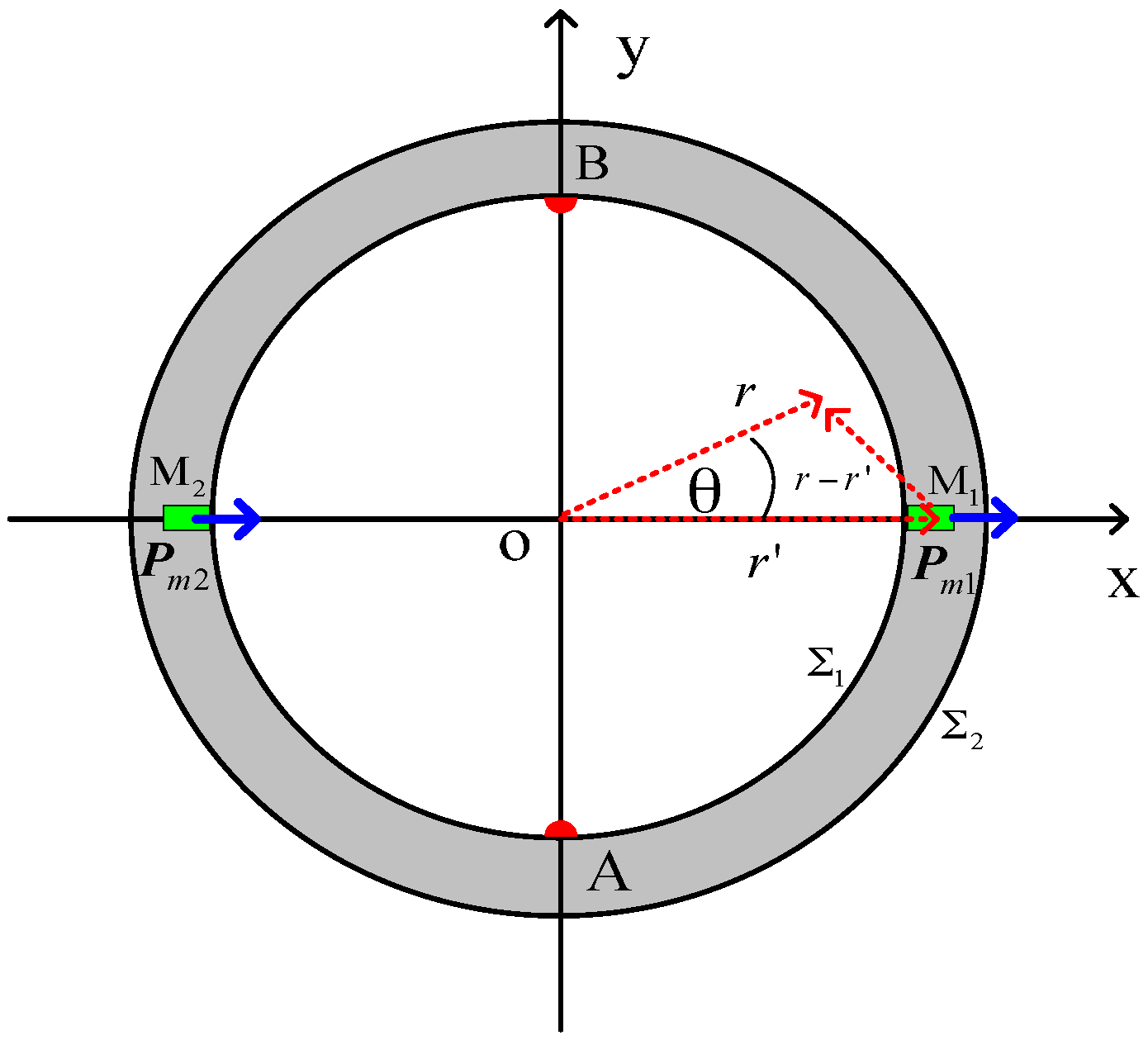
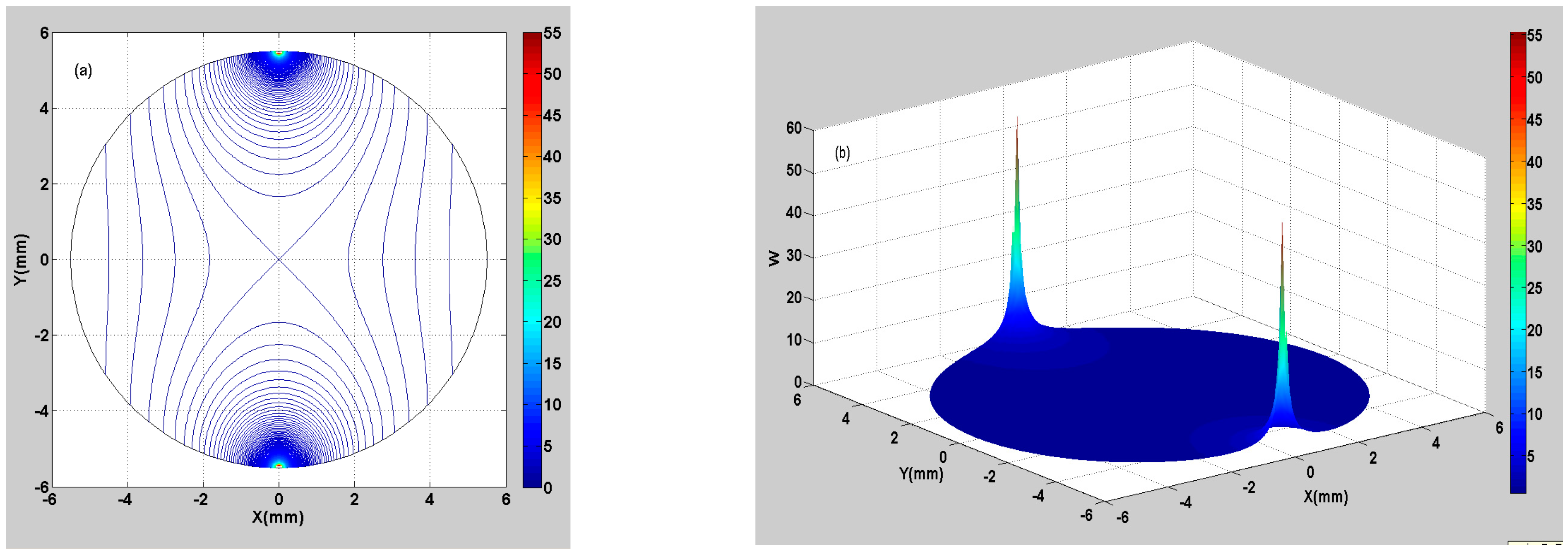
2.2. Weight Function of the Two-Electrode EMF
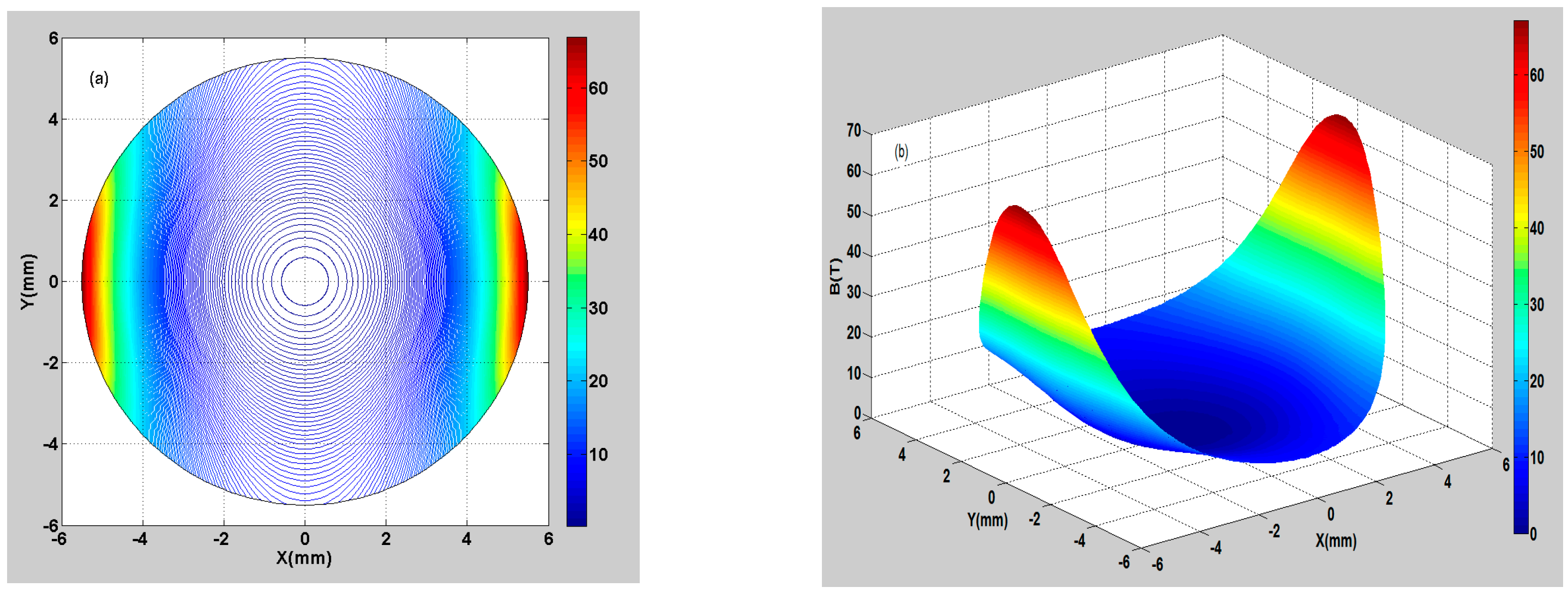
2.3. Magnetic Field of the Two-Electrode EMF
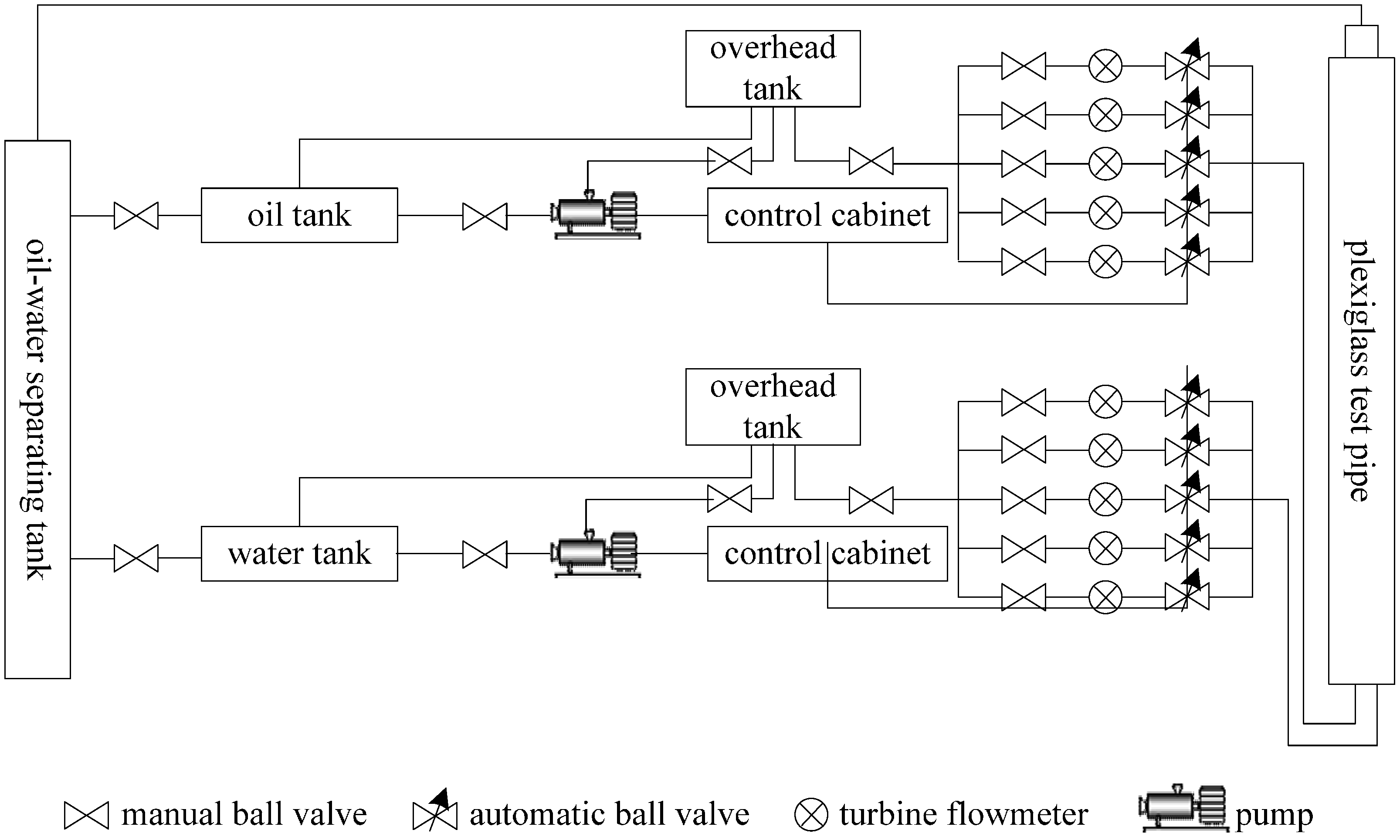
3. Dynamic Experiments on Multiphase Flow Loop Facility
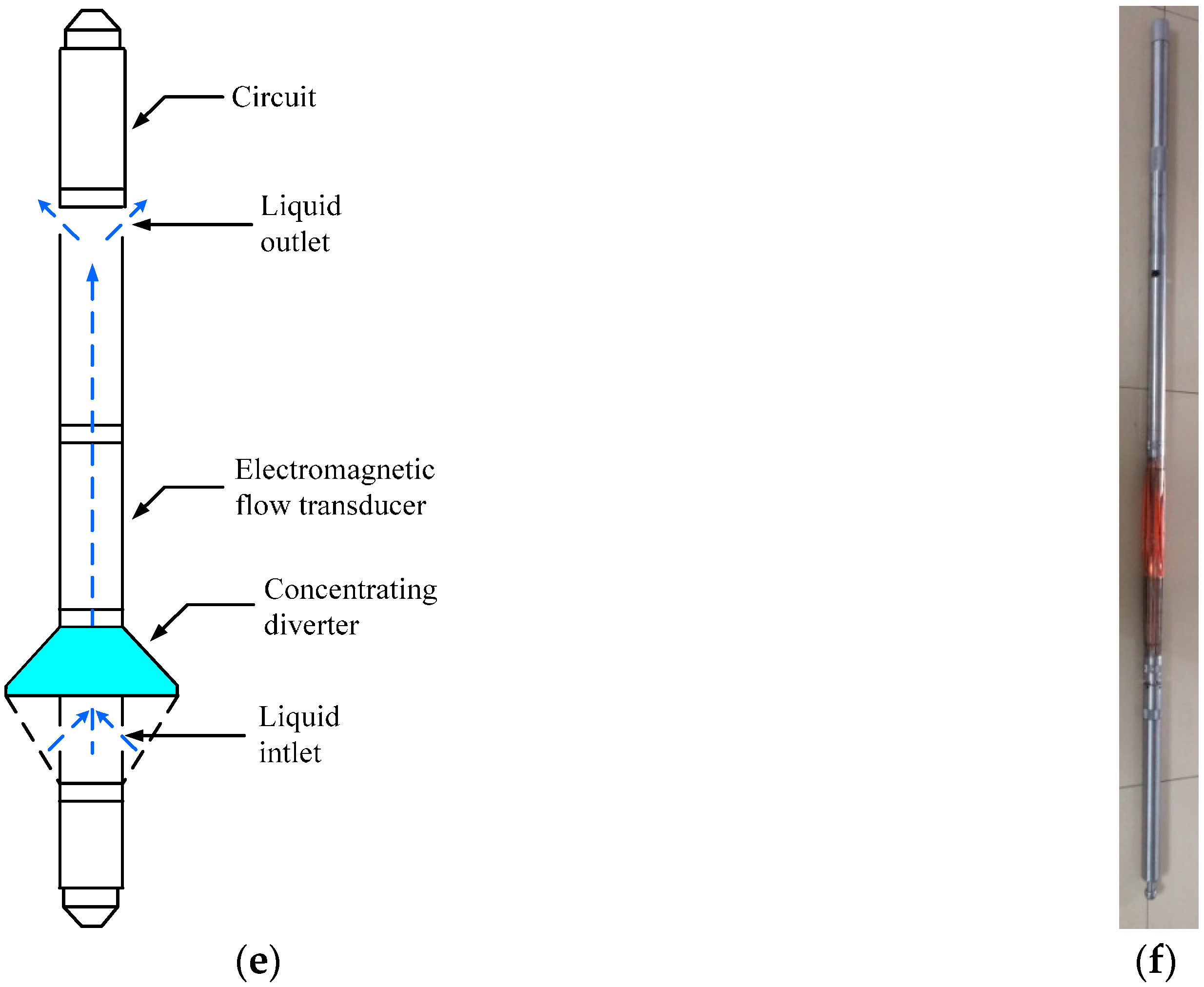
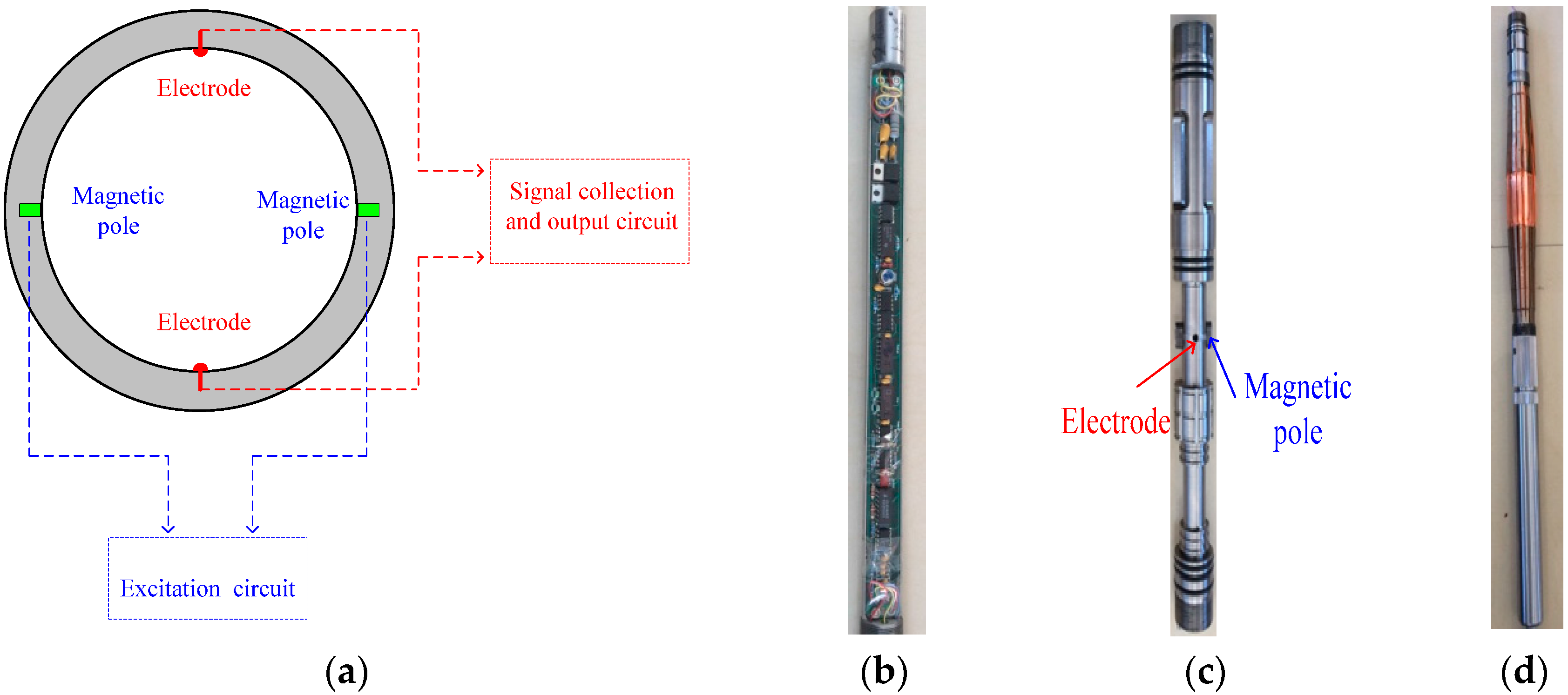
3.1. The Downhole Inserted Two-Electrode EMF
3.2. Experimental Design
3.3. Experimental Setup
3.4. Response Characteristics of the Two-Electrode EMF in Oil-Water Two-Phase Flow
- (1)
- Calculating the average value of the measurement data by Equation (29),where and represent the response frequency and the average response frequency of the electromagnetic flow transducer, respectively.
- (2)
- Calculating the standard deviation of the measurement data by Equation (30),where represents the standard deviation.
- (3)
- If , are treated outlier and excluded. Then, the average value and the standard deviation are re-calculated, respectively.
4. Onsite Experiments
5. Conclusions
- (1)
- The measurement principle, the weight function, and the magnetic field of the novel downhole inserted EMF are described.
- (2)
- Dynamic experiments on two EMFs in oil-water two-phase flow are carried out, and the experimental errors are analyzed in detail. The data analysis results of the dynamic experiments show that the EMF can be used for flowrate measurement of oil-water two-phase flow for the high-water-cut condition.
- (3)
- Furthermore, onsite experiments in high-water-cut oil-producing wells are conducted. The possible reasons for the errors in onsite experiments are analyzed. The results indicate that the EMF can provide an effective technology for measuring downhole oil-water two-phase flow.
Acknowledgments
Author Contributions
Conflicts of Interest
References
- Liu, X.B.; Wang, Y.J.; Xie, R.H.; Zhang, Y.H.; Huang, C.H.; Li, L. Novel Four-Electrode Electromagnetic Flowmeter for the Measurement of Flowrate in Polymer-Injection Wells. Chem. Eng. Commun. 2016, 203, 37–46. [Google Scholar] [CrossRef]
- Shercliff, J.A. The Theory of Electromagnetic Flow-Measurement; Cambridge University Press: Cambridge, UK, 1962; pp. 282–311. [Google Scholar]
- Wyatt, D.G. Electromagnetic flowmeter sensitivity with two-phase flow. Int. J. Multiphase Flow 1986, 12, 1009–1017. [Google Scholar] [CrossRef]
- Zhang, X.Z. Solution for the weighting function of electromagnetic flowmeters in two-dimensional concentric and eccentric annular flows. J. Hohai Univ. 1988, 16, 122–127. [Google Scholar]
- Zhang, X.Z. The effect of the phase distribution on the weight function of an electromagnetic flow meter in 2D and in the annular domain. Meas. Sci. Technol. 1997, 8, 1285–1288. [Google Scholar] [CrossRef]
- Wang, Z.H.; Wang, P.Z.; Lu, C.L. Field and Wave Electromagnetics; Publishing House of Electronics Industry: Beijing, China, 2000; pp. 102–106. [Google Scholar]
- Wang, J.Z.; Tian, G.Y.; Lucas, G.P. Relationship between velocity profile and distribution of induced potential for an electromagnetic flow meter. Flow Meas. Instrum. 2007, 18, 99–105. [Google Scholar] [CrossRef]
- Tewodros, A. Design of an electromagnetic flowmeter for insulating liquids. Meas. Sci. Technol. 1999, 10, 755–758. [Google Scholar]
- Wang, B.L.; Fu, Y.F.; Huang, Z.Y.; Li, H.Q. Volumetric flowrate measurement with capacitive electromagnetic flowmeter in oil-water two-phase flow. In Proceedings of the IEEE 2010 Instrumentation and Measurement Technology Conference, Austin, TX, USA, 3–6 May 2010; pp. 775–778.
- Bernier, R.N.; Brennen, C.E. Use of the electromagnetic flowmeter in a two-phase flow. Int. J. Multiph. Flow 1983, 9, 251–257. [Google Scholar] [CrossRef]
- Mi, Y.; Ishii, M.; Tsoukalas, L.H. Investigation of vertical slug flow with advanced two-phase flow instrumentation. Nucl. Eng. Des. 2001, 204, 69–85. [Google Scholar] [CrossRef]
- Jae-Eun, C.; Yeh-Chan, A.; Kyung-Woo, S.; Ho, Y.N.; Jong, H.; Moo, H.K. The performance of electromagnetic flowmeters in a liquid metal two-phase flow. J. Nucl. Sci. Technol. 2003, 40, 744–753. [Google Scholar]
- Hemp, J.; Sanderson, M.L.; Koptioug, A.V.; Liang, B.; Sweetland, D.J.; Al-Rabeh, R.H. Problems in the theory and design of electromagnetic flowmeters for dielectric liquids Part 1: Experimental assessment of static charge noise levels and signal-to-noise ratios. Flow Meas. Instrum. 2002, 13, 143–153. [Google Scholar] [CrossRef]
- Rosales, C.; Sanderson, M.L.; Hemp, J. Problems in the theory and design of electromagnetic flowmeters for dielectric liquids. Part 2a: Theory of noise generation by turbulence modulation of the diffuse ionic charge layer near the pipe wall. Flow Meas. Instrum. 2002, 13, 155–163. [Google Scholar] [CrossRef]
- Rosales, C.; Sanderson, M.L.; Hemp, J. Problems in the theory and design of electromagnetic flowmeters for dielectric liquids. Part 2b: Theory of noise generation by charged particles. Flow Meas. Instrum. 2002, 13, 165–171. [Google Scholar] [CrossRef]
- Cui, W.H.; Li, B.; Chen, J.; Li, X.W. A Novel Method of Multi-Information Acquisition for Electromagnetic Flow Meters. Sensors 2016, 16, 25. [Google Scholar] [CrossRef] [PubMed]
- Stelian, C. Calibration of a Lorentz force flowmeter by using numerical modeling. Flow Meas. Instrum. 2013, 33, 36–44. [Google Scholar] [CrossRef]
- Laogun, A.A.; Newman, D.L.; Gosling, R.G. Comparison of pulse wave velocity measured by doppler shifted ultrasound and electromagnetic flowmetry. Ultrasound Med. Biol. 1978, 3, 367–371. [Google Scholar] [CrossRef]
- De Oliveira, E.C.; Monteiro, M.I.; Pontes, F.V.; de Almeida, M.D.; Carneiro, M.C.; Da Silva, L.I.; Neto, A.A. Impact of the analytical blank in the uncertainty evaluation of the copper content in waters by flame atomic absorption spectrometry. J. AOAC Int. 2012, 95, 560–565. [Google Scholar] [CrossRef] [PubMed]
- De Oliveira, E.C. Simplified calibration methodology of chromatographs used in custody transfer measurements of natural gas. Metrol. Meas. Syst. 2012, 19, 405–416. [Google Scholar] [CrossRef]


| Source of Variation | Sum of Squares (Hz2) | Degrees of Freedom | Variance (Hz2) | F | Significance |
|---|---|---|---|---|---|
| Regression, REG | SSREG: 14,670,981.14 | 1 | 14,670,981.14 | 9138.56 | F0.01: 7.31 |
| Lack of fit, LOF | SSLOF: 28,333.51 | 8 | 3541.69 | 1.02 | F0.01: 2.99 |
| F0.1: 1.83 | |||||
| Pure error, PE | SSPE: 173,091.59 | 50 | 3461.83 | - | - |
| Total | SST: 14,779,584.29 | 59 | - | - | - |
| Source of Variation | Sum of Squares (Hz2) | Degrees of Freedom | Variance (Hz2) | F | Significance |
|---|---|---|---|---|---|
| Regression, REG | SSREG: 12,182,370.25 | 1 | 12,182,370.25 | 2934.80 | F0.01: 7.31 |
| Lack of fit, LOF | SSLOF: 33,009.10 | 7 | 4715.59 | 1.14 | F0.01: 3.29 |
| F0.1: 1.83 | |||||
| Pure error, PE | SSPE: 186,795.50 | 45 | 4151.01 | - | - |
| Total | SST: 12,402,174.85 | 53 | - | - | - |
| Water-Cut | 100% | 90% | 80% | 70% | 60% | 50% | |
|---|---|---|---|---|---|---|---|
| Flowrate | |||||||
| 60 m3/d | 0.01% | 0.70% | −1.06% | −1.90% | 0.84% | 1.17% | |
| 55 m3/d | −1.72% | 0.03% | 0.93% | 1.62% | 0.47% | 0.08% | |
| 50 m3/d | 0.27% | 0.94% | 0.93% | 1.33% | 1.57% | 0.79% | |
| 40 m3/d | 1.40% | 4.21% | 4.20% | 3.60% | 3.56% | 3.00% | |
| 30 m3/d | 1.09% | 2.36% | 2.48% | 2.49% | 2.08% | 0.61% | |
| 20 m3/d | −0.03% | 0.79% | 0.92% | 1.13% | −0.14% | −8.72% | |
| 10 m3/d | −0.48% | −0.53% | −1.99% | 0.14% | 1.13% | −6.57% | |
| 5 m3/d | −0.13% | −3.78% | 2.18% | −0.33% | −4.50% | 5.93% | |
| 3 m3/d | −0.62% | −4.91% | −5.03% | 11.84% | 11.98% | −4.35% | |
| 2 m3/d | −0.11% | −2.73% | −6.48% | 18.37% | 19.26% | −40.78% | |
| Water-Cut | 100% | 90% | 80% | 70% | 60% | 50% | |
|---|---|---|---|---|---|---|---|
| Flowrate | |||||||
| 60 m3/d | −2.87% | −2.56% | −2.44% | −3.08% | −2.27% | −3.86% | |
| 55 m3/d | −3.36% | −2.05% | −1.42% | −1.09% | −1.43% | −4.90% | |
| 50 m3/d | 1.06% | 1.86% | 2.17% | 3.57% | 3.65% | −0.52% | |
| 40 m3/d | 3.24% | 4.29% | 4.10% | −0.73% | −0.66% | −0.44% | |
| 30 m3/d | 3.19% | −0.70% | −0.74% | −0.89% | −1.01% | −1.38% | |
| 20 m3/d | −1.61% | −0.84% | −0.46% | −0.09% | −0.78% | −3.86% | |
| 10 m3/d | −1.12% | −0.67% | −0.28% | −1.55% | −0.50% | −5.48% | |
| 5 m3/d | −0.19% | 0.05% | −0.36% | −0.65% | 2.64% | 1.17% | |
| 2 m3/d | −1.17% | 3.02% | 6.86% | 25.54% | 30.39% | 47.88% | |
| Test Depth (m) | Perforated Zone | Turbine Flowmeter | No. 1 EMF | ||||
|---|---|---|---|---|---|---|---|
| First (m3/d) | Second (m3/d) | Third (m3/d) | First (m3/d) | Second (m3/d) | Third (m3/d) | ||
| 1083.4 | X1 | 34.6 | 34.9 | 34.9 | 52.2 | 52.2 | 52.3 |
| 1095.9 | X2 | 13.9 | 14.1 | 14.0 | 22.5 | 22.5 | 22.2 |
| 1100.7 | X3 | 5.4 | 5.6 | 5.8 | 10.8 | 10.4 | 10.6 |
| 1106.6 | X4 | 2.1 | 2.4 | 2.2 | 5.2 | 5.5 | 5.8 |
| 1180.0 | bore-hole bottom | 0 | 0 | 0 | 0 | 0 | 0 |
| Test Depth (m) | Perforated Zone | Turbine Flowmeter | No. 2 EMF | ||||
|---|---|---|---|---|---|---|---|
| First (m3/d) | Second (m3/d) | Third (m3/d) | First (m3/d) | Second (m3/d) | Third (m3/d) | ||
| 1030.3 | Y1 | 0 | 0 | 0 | 37.0 | 37.3 | 37.8 |
| 1036.7 | Y2 | 0 | 0 | 0 | 15.7 | 15.5 | 15.1 |
| 1045.2 | Y3 | 0 | 0 | 0 | 10.8 | 10.4 | 10.6 |
| 1055.0 | Y4 | 0 | 0 | 0 | 7.4 | 7.1 | 7.8 |
| 1139.9 | bore-hole bottom | 0 | 0 | 0 | 0 | 0 | 0 |
© 2016 by the authors; licensee MDPI, Basel, Switzerland. This article is an open access article distributed under the terms and conditions of the Creative Commons Attribution (CC-BY) license (http://creativecommons.org/licenses/by/4.0/).
Share and Cite
Wang, Y.; Li, H.; Liu, X.; Zhang, Y.; Xie, R.; Huang, C.; Hu, J.; Deng, G. Novel Downhole Electromagnetic Flowmeter for Oil-Water Two-Phase Flow in High-Water-Cut Oil-Producing Wells. Sensors 2016, 16, 1703. https://doi.org/10.3390/s16101703
Wang Y, Li H, Liu X, Zhang Y, Xie R, Huang C, Hu J, Deng G. Novel Downhole Electromagnetic Flowmeter for Oil-Water Two-Phase Flow in High-Water-Cut Oil-Producing Wells. Sensors. 2016; 16(10):1703. https://doi.org/10.3390/s16101703
Chicago/Turabian StyleWang, Yanjun, Haoyu Li, Xingbin Liu, Yuhui Zhang, Ronghua Xie, Chunhui Huang, Jinhai Hu, and Gang Deng. 2016. "Novel Downhole Electromagnetic Flowmeter for Oil-Water Two-Phase Flow in High-Water-Cut Oil-Producing Wells" Sensors 16, no. 10: 1703. https://doi.org/10.3390/s16101703
APA StyleWang, Y., Li, H., Liu, X., Zhang, Y., Xie, R., Huang, C., Hu, J., & Deng, G. (2016). Novel Downhole Electromagnetic Flowmeter for Oil-Water Two-Phase Flow in High-Water-Cut Oil-Producing Wells. Sensors, 16(10), 1703. https://doi.org/10.3390/s16101703