A Parallel Algorithm for Scheduling a Two-Machine Robotic Cell in Bicycle Frame Welding Process

Featured Application

The proposed method can be applied to optimize welding stations with two or more positioners for each welding robot. Such robotic cells ares used, e.g., in welding aluminum bicycle frames.

Abstract

Welding frames with differing geometries is one of the most crucial stages in the production of high-end bicycles. This paper proposes a parallel algorithm and a mixed integer linear programming formulation for scheduling a two-machine robotic welding station. The time complexity of the introduced parallel method is $O\left({log}^{2}n\right)$ on an $n^3$-processor Exclusive Read Exclusive Write Parallel Random-Access Machine (EREW PRAM), where n is the problem size. The algorithm is designed to take advantage of modern graphics cards to significantly accelerate the computations. To present the benefits of the parallelization, the algorithm is compared to the state of art sequential method and a solver-based approach. Experimental results show an impressive speedup for larger problem instances—up to 314 on a single Graphics Processing Unit (GPU), compared to a single-threaded CPU execution of the sequential algorithm.

1. Introduction

Scheduling problems are strongly connected to real-life production systems. Especially for cyclic (periodic) manufacturing, even a small improvement achieved by using dedicated algorithms can lead to significant profits. Job scheduling problems in flexible production systems are a particularly interesting subject of research, as indicated by numerous publications analyzed in the literature reviews [1,2,3]. Optimization often involves not only the assignment of operations (jobs) to machines, but also the order in which they are performed. Exact algorithms such as Mixed Integer Programming (MIP) [4] can be used to solve some (usually simpler) problems. For the NP-difficult ones, for instance, the Traveling Salesman Problem [5], the Knapsack Problem [6] or the Vehicle Routing Problem [7,8], the most common tools for solving them are heuristic algorithms. As shown for flexible the Job Shop Scheduling Problem (JSSP) in [3,9] or Dynamic JSSP [10], hybrid solutions, based on combining different algorithms to achieve the best possible results, are a common choice. An exemplary hybrid algorithm could utilize a two-level optimization schema:

Level 1

The order in which jobs are processed in the system.

Level 2

Jobs to machines assignment.

Two-level metaheuristics were successfully used to solve scheduling problems [11,12]. Alternatively, one can solve the first level conventionally and treat the second level as the so-called very large-scale neighborhood [13,14].

This paper discusses the problem of assigning jobs to machines in a two-machine robotic cell, where the order of jobs is determined (Level 2). Prior to each job, a setup is performed, the length of which depends on the previous job performed on the machine. The problem is inspired by the frame welding in a bicycle factory located in Poland.

The factory produces four types of aluminum bicycle frames: Mountain, trekking, city and children’s. Moreover, some of the frames are produced in two variants—male and female. The lengths and diameters of the components additionally depend on the dimensions of the frame, which can be standardized or customized on request. The key production stage is welding the frame elements, which is done in a robotic cell (see Figure 1). The cell consists of a welding robot, two positioners and storage fields for product components and ready-made bicycle frames. The frame welding process consists of three stages:

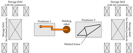
Figure 1. Robotic cell for aluminum bicycle frames welding.

• Move the frame elements from the storage field with kit containers and fix them in the positioner. The step is performed by a human operator, and—for safety reasons—with the robot disabled.
• Perform the welding job by the robotic arm. The time required to complete the job depends on the type and the size of the frame and the parameters of the positioner used. Human operator cannot enter the cell.
• Retrieve the finished frame and store it in a dedicated field. The step is performed by a human operator, and—for safety reasons—with the robot disabled.

The unique feature of the considered problem is that both jobs and setups occupy the robotic cell exclusively (i.e., there is one operator—human or robotic). A batch of products (with a predefined mixture) is manufactured repeatedly, until the demand changes. The problem will be referred to as the Cyclic Assignment Problem (CAP). The CAP corresponds to the second level of the previously described hybrid metaheuristic schema.

A sequential, exact algorithm for CAP was proposed in [12]. Unfortunately, despite the polynomial computational complexity, its execution time for CAP instances with a large number of jobs may be unacceptable in practice. Moreover, if the order of jobs also needs to be determined, a fast CAP solving algorithm could be used as a part of a two-stage metaheuristic. This paper presents a parallel exact algorithm designed to employ multi-processor environments, such as modern Graphic Processing Units (GPUs), drastically reducing the computation time required to solve larger problem instances. The main contributions can be summarized as follows:

• A new, parallel algorithm for CAP is proposed, suitable for an execution in a multi-processor environment (e.g., on a GPU).
• A formal analysis of the proposed algorithm is performed, showing $O\left({log}^{2}n\right)$ time complexity on a $n^3$-processor Exclusive Read Exclusive Write Parallel Random-Access Machine (EREW PRAM), where n is the number of jobs in a single production cycle.
• A Mixed Integer Linear Programming (MILP) model for CAP is proposed and its performance is discussed. The model is solved by a commercial software; with several standard improvement techniques tested, such as: Hot start, presolving, constraints reduction and providing bounds.

The rest of the paper is organized as follows. Section 2 contains a review of related work. Section 3 provides a definition and a mathematical model for the considered problem (CAP). Section 4 contains MILP formulation for CAP. The sequential state-of-art algorithm for CAP is summarized in Section 5, along with the graph model it utilizes. The new, parallel algorithm introduced in this paper is presented and analyzed theoretically in Section 6. Section 7 contains a description of the computational evaluation of the proposed algorithm. Finally, the concluding remarks are in Section 8.

2. Related Work

The problem discussed in this article—CAP—can be considered from the perspective of various classical classes of optimization problems, such as: Robotic cells, flexible production systems or cyclical scheduling. In addition, the unique element of CAP is the presence of additional constraints on the production resources (a single operator and setups). This section summarizes the related literature in each of the fields mentioned.

2.1. Robotic Cells

A practical implementation of CAP may be, as presented in the motivation, a single robotic arm handling multiple machines (constituting a robotic cell). Optimization of manufacturing processes where robots are used is a separate and interesting problem, where two- [15,16] and three-machine [17] cases are often investigated. Multi-arm robotic cells are also considered [18,19], however this topic lies outside the scope of the paper.

A typical robotic cell variant and solving methods are presented in the paper [20]. There, a Flow Shop Scheduling Problem (FSSP) in a multi-machine robotic cell with a single robot was considered. The problem is NP-difficult, thus it was solved not only with Mixed Integer Programming (MIP), but also a parallel, hybrid heuristics based on a taboo search and a genetic algorithm. The influence of how cyclic production is defined on the overall efficiency was also investigated. Another classic approach to modeling robotic cells are Petri nets, the method favored when a complex, cyclic systems are considered. For example, in [21], a robotic cell with one robot was tackled, using the Petri nets variant (Timed Petri Nets, TPN). The initial TPN model was optimized with the LINGO solver to obtain the optimal solution (sequence of robot movements).

A potentially promising field for research in robotic cell scheduling (and optimization in general) is the use of Machine Learning (ML). While ML is a huge success in computer vision and natural language processing, the applications in operations research are currently relatively limited. Recent papers show a lot of interest in applying Reinforcement Learning (RL) for scheduling problems. For example, the reward function modeling was discussed in [22], where RL was used directly to optimize gantry cells. The empirical experiments showed, that the Q-learning performance varied depending on the function definition, with the rewards based on the problem properties outperforming others. A different angle for integrating RL was investigated in [23], where the technique was used as a part of classic solving method. The hybrid method performed better than a purely RL approach.

2.2. Cyclic and Flexible Production

The considered problem can be seen as a cyclic, flexible production system with single-operation jobs. Cyclic scheduling problems are commonly researched, as they can model mass-production, key in the global economy. Many classic multi-machine scheduling problems have cyclic variants [24]. For a comprehensive survey of models, algorithms and solvability analysis, refer, e.g., to [25].

While the classic scheduling problems are not obsolete; the attention of researchers is currently focused on solutions closer to the industrial applications. These, in the face of a more diversified and changing market demand, lean towards flexible production [26]. The recent reviews on flexible counterparts of FSSP [27] or Job Shop Scheduling Problem (JSSP) [28] present a vast body of literature. Vast enough to induce specialized surveys, such as [29], where swarm intelligence and evolutionary algorithms in JSSP were discussed exclusively.

The solving methods used are diverse, with Mathematical Programming and metaheuristics being most prominent. For example, in [30] a flexible FSSP with m identical machines was considered. The solution was based on a MILP formulation; authors proposed a reduced model that is more computationally efficient than the previously known ones. A heuristic approach was chosen in the study of flexible FSSP with some additional constraints was presented in [31]. The problem was solved with an iterated, greedy metaheuristics, in 4 phases. The first phase generates the initial solution using NEH heuristics [32], or randomly. Second phase disturbs the solution, improving exploratory properties. Third phase fixes the solution destructed in the second phase, while the fourth phase uses a descend neighborhood search to find the final solution. Paper [33] describes minimizing makespan and total tardiness for a flexible JSSP with sequence-dependent setup times that account for machine operators qualifications. The authors developed both exact branch-and-cut algorithm and a heuristic-based approach. The multi-stage approach showed a dominant performance both on randomly generated and real-world instances.

2.3. Additional Problem Constraints

Modeling real production systems entails considering many additional constraints for the problems. They may refer to the presence of certain limited resources at different stages of manufacturing, such as for example: Workers available, transport carts or robotic arms. Typical elementary events requiring the presence of an additional resources are: Transportation, performing operations (processing jobs) on machines and setups.

The variant in which the operations require resources, and optimization of their allocation is part of the problem [34], is particularly often analyzed [35]. One of the first works where the resource is discrete is [36]. There, the authors solved a FSSP with a limited pool of resources. For a review of a more recent research addressing such constraints, refer, e.g., to [37].

The case where the resource constraints are imposed only on the setups is relatively rarely considered in the literature. In one of the recently published works [4], the authors solved the problem of minimizing the makespan for Parallel Machines with disjoint setups. The proposed solution was based on the MILP model, Constraint Programming (CP) and dedicated heuristics. In [38], the problem of scheduling jobs on heterogeneous, parallel machines was investigated; in which the time of setups depended, among others, on the allocation of non-renewable resources. However, a limited number of simultaneous setups was not considered. MILP and dedicated heuristics were used again as the solving methods. Similarly, Integer Programming and CP (alongside a heuristics) were used in [39] to solve the problem with realistic energy constraints on setups. A variant of lotsizing problem was solved in [40]. The problem included sequence-dependent setups with an operator shared between the machines. Again, the solving method was based on Mathematical Programming and a commercial solver. Finally, a two-machine FSSP with disjoint, sequence-dependend setups was researched in [41]. The authors derived several problem properties, which they incorporated into a MILP formulation and a dedicated greedy algorithm.

3. Problem Definition

Cycling Assignment Problem (CAP) considers a robotic cell consisting of m machines (here, $m=2$ is usually assumed). The cell is processing n jobs from a set $\mathcal{J}=\{1,2,\dots ,n\}$ in a repetitive manner, i.e., each job $i\in \mathcal{J}$ must be processed precisely every T time (called cycle time). The processing cycles cannot overlap and the order of jobs is fixed, however each job can be processed on any chosen machine (the same in every cycle). The assignment of jobs to machines is given by $P\in \mathcal{P}$, where $P\left(i\right),i\in \mathcal{J}$ denotes a machine a job i is assigned to and $\mathcal{P}$ is a set of all possible assignments. Jobs processing times depend on the assigned machines, for a job $i\in \mathcal{J}$ the processing time on machine $a\in \mathcal{M}$ is given by $p_i^a$. Between any two jobs $i,j\in \mathcal{J}$, processed one after another on a machine $a\in \mathcal{M}$, there is a setup with a duration $s_{i\to j}^a$. Lastly, at most a single job or a single setup can be performed in the cell simultaneously and both job processing and setups are uninterruptible. The problem is to find $P\in \mathcal{P}$ allowing to minimize cycle time T.

Let $S_i^k$ and $C_i^k$ denote start and completion times of job $i\in \mathcal{J}$ in k-th production cycle of some schedule. The schedule is feasible iff the aforementioned problem constraints are satisfied, which can be formalized as follows:

$$\begin{array}{cc}\hfill \forall i\in \mathcal{J}\setminus \left\{n\right\}& S_{i+1}^k\ge S_i^k+p_i^{P\left(i\right)}+\mathit{setup}(P,i+1),\hfill \end{array}$$

(1)

$$\begin{array}{cc}\hfill \forall i\in \mathcal{J}& C_i^k=S_i^k+p_i^{P\left(i\right)},\hfill \end{array}$$

(2)

$$\begin{array}{cc}\hfill \forall i\in \mathcal{J}& S_i^{k+1}=S_i^k+T,\hfill \end{array}$$

(3)

$$\begin{array}{cc}& \hfill S_1^{k+1}\ge C_n^k+\mathit{setup}(P,1),\end{array}$$

(4)

where $\mathit{setup}(P,i)$ is a setup time before operation i according to assignment P,

$$\begin{array}{cc}\hfill \mathit{setup}(P,i)& =\{\begin{array}{cc}{s}_{max\mathcal{X}(P,i)}^{P\left(i\right)}\hfill & \mathrm{for}:\left|\mathcal{X}\right(P,i\left)\right|\ge 1,\hfill \\ s_{max\{j\in \mathcal{J}:P(i)=P(j\left)\right\}}^{P\left(i\right)}\hfill & \mathrm{otherwise},\hfill \end{array}\hfill \end{array}$$

(5)

$$\begin{array}{cc}\hfill \mathcal{X}(P,i)& =\{j\in \mathcal{J}:(j<i\wedge P\left(i\right)=P\left(j\right)\left)\right\}.\hfill \end{array}$$

(6)

For a given assignment $P\in \mathcal{P}$, it was shown in [12], that the minimal cycle time $T\left(P\right)$ for which a feasible schedule exists equals

$$T\left(P\right)=\sum _{i\in \mathcal{J}}\left(p_i^{P\left(i\right)}+\mathit{setup}(P,i)\right).$$

(7)

Therefore, the problem can be formulated as

$$\underset{P\in \mathcal{P}}{min}T\left(P\right)=\underset{P\in \mathcal{P}}{min}\sum _{i\in \mathcal{J}}\left(p_i^{P\left(i\right)}+\mathit{setup}(P,i)\right).$$

(8)

4. Mixed Integer Linear Formulation

In this section, a first MILP-formulation for CAP is introduced. Solving methods for scheduling problems commonly utilize MILP (e.g., refer to the related work in Section 2); and as such—this approach can constitute a valid point of reference for the presented dedicated exact algorithm.

The Equations (5), (6) and (8) define an objective function of CAP. They can be almost directly transformed into the following MILP formulation:

$$\underset{\mathbf{x},\mathbf{s}}{min}\sum _{a\in \mathcal{M}}\sum _{i\in \mathcal{J}}{\mathtt{x}}_i^a{p}_i^a+\sum _{i\in \mathcal{J}}{\mathtt{s}}_i,$$

(9)

subject to:

$$\begin{array}{cc}\hfill \forall i\in \mathcal{J}& \sum _{a\in \mathcal{M}}{\mathtt{x}}_i^a=1,\hfill \end{array}$$

(10)

$$\begin{array}{cc}\hfill \forall a\in \mathcal{M}\forall i,j\in \mathcal{J},j<i& {\mathtt{s}}_i\ge s_{j\to i}^a-\underset{0\mathrm{if}P\left(i\right)=P\left(j\right)=a}{\underbrace{M(2-{\mathtt{x}}_i^a-{\mathtt{x}}_j^a)}}-\underset{0\mathrm{if}j\mathrm{proceeds}i}{\underbrace{M\sum _{d=j+1}^{i-1}{\mathtt{x}}_d^a}},\hfill \end{array}$$

(11)

$$\begin{array}{cc}\hfill \forall a\in \mathcal{M}\forall i,j\in \mathcal{J},j\ge i& {\mathtt{s}}_i\ge s_{j\to i}^a-\underset{1\mathrm{if}P\left(i\right)=P\left(j\right)=a}{\underbrace{M(2-{\mathtt{x}}_i^a-{\mathtt{x}}_j^a)}}-\underset{0\mathrm{if}j\mathrm{proceeds}i}{\underbrace{M\left(\sum _{k=0}^{i-1}{\mathtt{x}}_k^a+\sum _{k=j+1}^n{\mathtt{x}}_k^a\right)}},\hfill \end{array}$$

(12)

where $M\in {\mathbb{R}}^{+}$ is a large number and $\mathbf{x}\in {\mathbb{Z}}^{m\times n}$ and $\mathbf{s}\in {\mathbb{R}}^n$ are decision variables. $\mathbf{x}$ encodes an assignment and for any $a\in \mathcal{M}$ and $i\in \mathcal{J}$,

$${\mathtt{x}}_i^a=\left\{\begin{array}{cc}1\hfill & \mathrm{if}\mathrm{job}i\mathrm{is}\mathrm{assigned}\mathrm{to}\mathrm{machine}a,\hfill \\ 0\hfill & \mathrm{otherwise}.\hfill \end{array}\right.$$

(13)

On the other hand, $\mathbf{s}$ encodes the duration of setups performed before the jobs, i.e., for any $i\in \mathcal{J}$, ${\mathtt{s}}_i=\mathit{setup}(P,i)$, where P must be consistent with $\mathbf{x}$. Constraint (10) ensures each job is assigned to exactly one machine. Constraints (11) and (12) are used to compute setup times before the jobs. For any machine $a\in \mathcal{M}$ and jobs $i,j\in \mathcal{J}$, the right hand side of the constraints is a negative number, except if according to the current $\mathbf{x}$, both job i and j are assigned to machine a and job j directly precedes i on a. Then, right side is equal to $s_{j\to i}^a$, thus ensuring the correct value of ${\mathtt{s}}_i$. Resulting MILP model consists of $2n$ binary and n continuous variables; and $n^2+n$ constraints.

When $m=2$, the number of variables and constraints can be further reduced easily. Consider the assignment encoded in ${\mathbf{x}}^{\prime }\in {\mathbb{Z}}^n$, with

$${\mathtt{x}}_i^{\prime }=\left\{\begin{array}{cc}0\hfill & \mathrm{if}\mathrm{job}i\mathrm{is}\mathrm{assigned}\mathrm{to}\mathrm{machine}1,\hfill \\ 1\hfill & \mathrm{if}\mathrm{job}i\mathrm{is}\mathrm{assigned}\mathrm{to}\mathrm{machine}2.\hfill \end{array}\right.$$

(14)

Then, one can substitute ${\mathtt{x}}_i^1≔-({\mathtt{x}}_i^{\prime }-1)$ and ${\mathtt{x}}_i^2≔{\mathtt{x}}_i^{\prime }$ in Equations (9), (11) and (12); then constrain ${\mathbf{x}}^{\prime }$ to be a vector of binary variables, instead of using (10). Reformulated MILP model consists of n binary and n continuous variables; and $n^2+n$ constraints (n constraints on ${\mathbf{x}}^{\prime }$ being binary, i.e., $n^2$ constraints and n bounds).

5. Sequential Algorithm

The purpose of this section is to provide an overview of the sequential algorithm for CAP introduced in [12] and the accompanying graph model. The algorithm will be further used to develop its parallel variant and as a baseline to compute a speedup.

5.1. Graph Model

A graph model for a two-machine CAP was first introduced and analyzed in [12], where it was used to build the exact solving algorithm. For the completeness, the model is summarized below. Note that $m=2$ is assumed.

Let $\mathcal{A}=(V,E)$ be a directed graph, where $V=\mathcal{W}\cup {\mathcal{W}}^{\prime }$ is a set of nodes and $E=\mathcal{E}\cup {\mathcal{E}}^{\prime }\cup {\mathcal{E}}^{″}$ is a set of arcs, where:

$$\begin{array}{cccc}\hfill \mathcal{W}& =\bigcup _{i\in \mathcal{M}}\bigcup _{j=1}^n\left\{(j,i)\right\},\hfill & \hfill {\mathcal{W}}^{\prime }& =\bigcup _{i\in \mathcal{M}}\bigcup _{j=n+1}^{2n}\left\{(j,i)\right\},\hfill \end{array}$$

(15)

$$\begin{array}{cccc}\hfill \mathcal{E}& =\bigcup _{a\in \mathcal{M}}\bigcup _{i=1}^{n-1}\bigcup _{j=i+1}^n\left\{\left((i,a),(j,\overline{a})\right)\right\},\hfill & \hfill {\mathcal{E}}^{\prime }& =\bigcup _{a\in \mathcal{M}}\bigcup _{i=2}^n\bigcup _{j=n}^{n-1+i}\left\{\left((i,a),(j,\overline{a})\right)\right\},\hfill \end{array}$$

(16)

$$\begin{array}{cccc}\hfill {\mathcal{E}}^{″}& =\bigcup _{a\in \mathcal{M}}\left\{\left((n,a),(2n,a)\right)\right\},\hfill & \hfill \overline{a}& =\left\{\begin{array}{cc}1\hfill & \mathrm{if}a=2,\hfill \\ 2\hfill & \mathrm{if}a=1.\hfill \end{array}\right.\hfill \end{array}$$

(17)

Example 1.

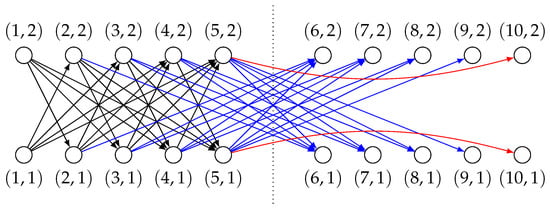
Consider CAP instance with $n=5$ and $m=2$. The corresponding graph $\mathcal{A}$ is shown in Figure 2. Arcs from the set $\mathcal{E}$ are marked in black, arcs from the set ${\mathcal{E}}^{\prime }$ are marked blue and arcs from the set ${\mathcal{E}}^{″}$ are marked red.

Figure 2. Graph $\mathcal{A}$ for CAP instance with $n=5$ and $m=2$.

Any node $(i,a)\in V$ represents a job i or $i-n$ (depending on the cycle), performed on a machine a. Arcs, on the other hand, represent sequences of jobs assigned to the same machine, preceded by a job assigned to a different machine. More precisely, any arc $\left(\right(i,a),(j,b\left)\right)\in E$ corresponds to a sequence of assignments $P\left(i\right)=a$, $P(i+1)=b$, …, $P(j-1)=b$, $P\left(j\right)=b$, if $i,j\le n$. For $j>n$, the indexes of assignments beyond n are reduced by n (refer to Example 2).

Nodes are unweighted, while the weight of arcs reflect the duration of the jobs and setups they represent. To simplify the notation, the definition of job and setup durations is extended for all the indexes of nodes in $\mathcal{A}$

$$\begin{array}{cc}{s}_{i,j}^a≔s_{\left(\right(i-1)modn)+1,\left(\right(j-1)modn)+1}^a\hfill & \mathrm{for}:i,j>n,a\in \mathcal{M},\hfill \end{array}$$

(18)

$$\begin{array}{cc}{p}_i^a≔p_{\left(\right(i-1)modn)+1}^a\hfill & \mathrm{for}:i>n,a\in \mathcal{M}.\hfill \end{array}$$

(19)

For example, if $n=5$, then $p_{11}^1=p_1^1$ and $s_{2\to 6}^a=s_{2\to 1}^a$. With the extended indexing, the weights of arcs in $\mathcal{A}$ are given by

$$\begin{array}{c}\hfill d\left(\left(\right(i,a),(j,b\left)\right)\right)=p_i^a+s_{i,j+1}^a+\sum _{k=i+1}^{j-1}\left(p_k^b+s_{k,k+1}^b\right)\mathrm{for}:((i,a),(j,b))\in E.\end{array}$$

(20)

Definition 1.

Any path from $(i,a)$ to $(i+n,a)$ in graph $\mathcal{A}$, for any $a\in \mathcal{M}$, $i\in \mathcal{J}$, is called a highlighted path. A set of all such paths is denoted by $\mathcal{L}$.

Each highlighted path corresponds to exactly one assignment, and each assignment corresponds to exactly one highlighted path. An assignment corresponding to a given highlighted path can be constructed by transforming each arc in the path into its corresponding assignments (for a rigorous formula refer to [12]).

Example 2.

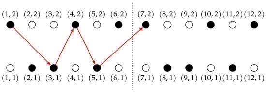
Consider a CAP instance with $n=6$ and $m=2$. A graph $\mathcal{A}$ build for this instance is shown on Figure 3. A highlighted path $\left((1,2),(3,1),(4,2),(5,1),(7,2)\right)$, constructed for $P=(2,1,1,2,1,2)$ is marked in red. Black dots represent job-machine assignments.

Figure 3. An example of a highlighted path (marked in red) for CAP instance with $n=6$ and $m=2$; the path corresponds to $P=(2,1,1,2,1,2)$.

Theorem 1

([12]). In graph $\mathcal{A}$, the weight of highlighted path with the minimum weight is equal to the minimal cycle time.

Based on Theorem 1, the highlighted paths can be used to find an optimal solution of CAP. Such method is described in the following subsection.

5.2. Algorithm Description

The sequential algorithm for CAP is based on the graph model presented in the previous section. The algorithm can be summarized in three steps:

• Build graph $\mathcal{A}$.
• Find highlighted path of the lowest weight $\mathbf{\mu }$.
• Transform $\mathbf{\mu }$ into an assignment.

Steps 1. and 3. are straightforward. Step 2. is equivalent to the problem of finding the path with the lowest weight in the graph among the paths connecting the pairs of nodes $(i,a)$ and $(i+n,a)$, for all $a\in \mathcal{M}$, $i\in \mathcal{J}$ (a total of $2n$ pairs). The $\mathcal{A}$ graph is an acyclic, directed graph with non-negative weights on the arcs. Hence, to find the mentioned path, one can use the All-Pairs Shortest Path (APSP) problem solving algorithm, and then choose the shortest of $2n$ paths, or solve Single-Source Shortest Path (SSSP) $2n$ times. The computational complexity of the algorithm is $O\left(n^3\right)$ [12].

6. Parallel Algorithm

In this section the new, parallel exact algorithm for CAP is introduced. The algorithm is described and analyzed theoretically in the context of the abstract machine EREW PRAM.

6.1. Algorithm Description

The algorithm is based on the sequential method proposed in [12] and is designed for computing machines with large number of processors and a shared memory that can be used for communication (e.g., GPUs). The pseudocode for the algorithm is presented in Algorithm 1.

In stage 1, the graph $\mathcal{A}$ is build in parallel. The procedure starts with calculating prefix sums to accelerate the computations later. In lines 1–3, setup times and processing times are copied to arrays $\mathtt{S}$ and $\mathtt{P}$. Then, in lines 4–5, prefix sums are computed

$$\mathtt{P}[a,i]=\sum _{k=1}^i{p}_k^a,\mathtt{S}[a,i]=\sum _{k=1}^i{s}_{k-1,k}^a,$$

(21)

for $a\in \mathcal{M}$ and $i\in \{1,2,\cdots ,2n\}$ (note the indexes up to $2n$). Prefix sums are used to calculate the weights of the graph $\mathcal{A}$, in lines 7–11. The weights are stored in a 4-dimensional array $\mathtt{D}$, such that for any arc $\left((i,a),(j,b)\right)\in E$,

$$\begin{array}{cc}\hfill \mathtt{D}[i,a,j,b]& =d\left(\left(\right(i,a),(j,b\left)\right)\right)\hfill \\ \hfill & =p_i^a+s_{i,j+1}^a+\sum _{k=i+1}^{j-1}\left(p_k^b+s_{k,k+1}^b\right).\hfill \\ \hfill & =p_i^a+s_{i,j+1}^a+\sum _{k=1}^{j-1}{p}_k^b-\sum _{k=1}^i{p}_k^b+\sum _{k=1}^{j-1}{s}_{k,k+1}^b-\sum _{k=1}^i{s}_{k,k+1}^b\hfill \\ \hfill & =p_i^a+s_{i,j+1}^a+\mathtt{P}[b,j-1]-\mathtt{P}[b,i]+\mathtt{S}[b,j]-\mathtt{S}[b,i+1].\hfill \end{array}$$

(22)

For any combination of indexes $i,j,a,b$, not representing a valid arc, an infinity is written into the array. Stage 1 is concluded, and the graph $\mathcal{A}$ is constructed, with its arcs represented in the array $\mathtt{D}$.

Algorithm 1: Parallel exact algorithm for CAP

The goal of stage 2 is to compute a highlighted path with the lowest weight. For this purpose, APSP is solved in line 12 (by a chosen algorithm) in the graph $G=(V,E_g)$, described by $\mathtt{D}$. This graph has the same set of nodes as $\mathcal{A}$, however it is fully connected (a complete digraph). Graph G is analogous to $\mathcal{A}$, however non-existent arcs from $\mathcal{A}$ are represented by arcs with infinite weights:

$$d\left(\left(\right(i,a),(j,b\left)\right)\right)=\mathtt{D}[i,a,j,b],\mathrm{for}:\left((i,a),(j,b)\right)\in E_g.$$

(23)

It is assumed, that APSP solving algorithm writes distances between nodes into $\mathtt{D}$. Then, in line 13, a pair of nodes constituting a start and end of a highlighted path with lowest weight is computed. Finally, in line 14, the path is constructed. The exact method is derived from the APSP algorithm used.

Stage 3 of the algorithm transforms the highlighted path found in stage 2, into the optimal assignment. For the ease of presentation, the method is summarized in a separate pseudocode, in Algorithm 2.

Algorithm 2: Building an assignment corresponding to a highlighted path

The method is designed so that it can be performed on a machine where a concurrent memory access is impossible. First, in lines 2–4, a special case when all the jobs are assigned to the same machine is handled. Then, if it is not the case, basic information is broadcasted in parallel to each of n processors in line 5. The following code is performed on each processor separately. The Synchronize command indicates the place in the logic where the processors should synchronize the execution. It can be achieved, e.g., by placing Iddle commands so that each branch requires the same number of processor cycles. In lines 7–10, an array $\mathtt{P}$ is initialized. The array will contain the assignment constructed by the method. During the initialization, only the assignments directly contained in $\mathbf{\mu }$ are written. Other elements of the array are filled with $-1$. Similarly, an array $\mathtt{TO}$ is initialized in lines 12–18. The array contains information required to avoid conflicts during copying data into $\mathtt{P}$. Each element of $\mathtt{TO}$ contains a left-side bound a certain assignment should be copied up to. In other words, ignoring edge cases, if $\mathtt{TO}\left[i\right]=j$, then jobs from $j+1$ to i should be assigned to the machine $\mathtt{P}\left[i\right]$. The following part of the algorithm is divided into sequential steps, iterations of the loop in line 21. The number of steps is computed in line 20. In line 22, a shift is computed. The shift determines which element of $\mathtt{P}$ will be modified in a given step. Then, if a processor p is “active” (e.g., if $\mathtt{P}\left[p\right]\ne -1$) and left-side bound in $\mathtt{TO}$ is satisfied, a next value is written into $\mathtt{P}$ and $\mathtt{TO}$. Each step of the algorithm is concluded by a synchronization. Refer to Example 3 for a step-by-step analysis of the contents of $\mathtt{P}$ and $\mathtt{TO}$ during a run of the algorithm.

Example 3.

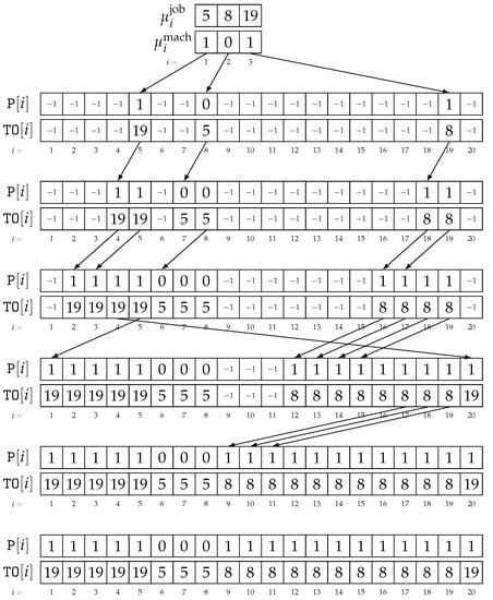
Consider CAP instance with $n=20$ and $m=2$. Let $\mathbf{\mu }=\left(\right(5,2),(8,1),(19,2\left)\right)$ be a highlighted path in the graph $\mathcal{A}$, constructed for this instance. Figure 4 shows the memory during the construction of the assignment corresponding to $\mathbf{\mu }$, using Algorithm 2. The first two rows represent the nodes of $\mathbf{\mu }$. The following two rows represent the state of arrays $\mathtt{P}$ and $\mathtt{TO}$ after synchronization in line 19. Each of the following pairs of rows represent the state after synchronizations in line 35. Finally, the arrows on the figure represent the write operations performed by the processors in each iteration of loop in line 21.

Figure 4. Memory during computations in Algorithm 2 for $n=20$ and $\mathbf{\mu }=\left(\right(5,2),(8,1),(19,2\left)\right)$.

6.2. Computational Complexity

Algorithms are usually analyzed theoretically in the context of the so-called abstract machines. They are simplified models of computer systems (in particular, the hardware), that allow to predict various properties of the software executed on real machines [42], such as computation time or memory requirements.

For the analysis, Parallel Random Access Machine (PRAM) [43,44] model will be used, which is an extension of the sequential RAM model. The PRAM model is one of the most widely used models of parallel machines ([45], pp. 18–19), and has been the subject of numerous scientific publications (examples of which can be found in ([46], pp. 74–76)).

In simple terms, the PRAM model assumes the existence of k processors having access to a shared memory of an unlimited size at a constant time. The processors have synchronized clocks, i.e., execute the instructions simultaneously, with each processor being allowed to execute a different instruction. The instructions are limited to read/write and simple local variable operations such as comparison or summation. Due to additional limitations related to the access to the shared memory, there are four general subclasses of PRAM models: EREW, CREW, ERCW and CRCW (in the abbreviations, “E” stands for exclusive, “C” for concurrent, “R” for read and “W” for write). In EREW PRAM, both read and write operations are exclusive, i.e., any memory cell can be accessed by a single processor at a time. The model is restrictive, but closely reassembles many hardware implementations. Another popular model is CREW PRAM, where concurrent read is allowed. CREW is a good approximation of systems where shared memory access is not a bottleneck. Note that any algorithm suitable for EREW, can also be executed on CREW. For that reason, EREW PRAM will be applied for the analysis whenever possible.

Lemma 1.

Consider a highlighted path in graph $\mathcal{A}$, build for a CAP instance with n jobs and $m=2$ machines. The corresponding assignment can be calculated in $O(logn)$ time on n-processor EREW PRAM.

Proof. 

The assignment corresponding to any highlighted path can be found using Algorithm 2, analyzed further for computational complexity on EREW PRAM. Assume there are n processors available. Broadcasting any scalar information from a single processor, to all processors can be performed in $O(logn)$ time (lines 3, 5). Then, a special case check in lines 2–4 can be performed in $O(logn)$ time. Operations in the main, parallel loop from lines 6–32 are designed to prevent conflicts in memory access. The synchronization is achieved by tuning the number of processor cycles for each branch in logic, which does not bring an additional overhead. Thus, operations in lines 7–20 take $O\left(1\right)$ time on n processors (assuming ${log}_{2}n$ can be computed in constant time, otherwise the operation would have to be performed outside the parallel region). Loop from lines 21–32 has $O(logn)$ iterations, and each can be performed in constant time on each processor. As a result, the final computational complexity of the algorithm is in $O(logn)$ on n-processor EREW PRAM.    □

Theorem 2.

Consider a CAP instance with n jobs and $m=2$ machines. The optimal solution for that instance can be found in

$$O\left(logn+T_{\mathrm{APSP}}\right)$$

time, on $max\{n^2,P_{\mathrm{APSP}}\}$-processor EREW PRAM, where $T_{\mathrm{APSP}}$, $P_{\mathrm{APSP}}$ are time and number of processors required to solve APSP on the graph $\mathcal{A}$ build for that instance.

Proof. 

The problem can be solved using Algorithm 1. The algorithm is divided into three stages. Stage one starts with calculating prefix sums. Write operations from lines 1–3 can be performed in $O(\lceil n/k\rceil )$ time on k processors (assigning 8 write operations for each processor). Prefix sums from lines 5 and 6 can be calculated in $O(logn)$ time on n-processor EREW PRAM [47]. Assume k processors are available for the parallel region in lines 7–11. There are several points in the execution where potential memory conflicts may arise: Comparison with n from line 8, read operation on job duration stored in p (line 9) and read operations on prefix sums $\mathtt{S}$, $\mathtt{P}$ (also line 9). Without considering the conflicts, the time complexity of the region is $O(\lceil n^2/k\rceil )$. With a maximal parallelism achieved with $k=n^2$, at most $O\left(n\right)$ processors can attempt to read $O\left(n\right)$ data cells at the same time. Thus, to avoid conflicts, it is enough to provide n copies of p, $\mathtt{S}$ and $\mathtt{P}$, which takes $O(logn)$ on $n^2$ processors. In total, with $n^2$ processors available, stage 1 takes $O(logn)$ time.

Stage 2 assumes a APSP solving algorithm is used. The graph in the problem consists of $O\left(n\right)$ nodes and $O\left(n^2\right)$ arcs. Let $T_{\mathrm{APSP}}$ be the time required to solve the APSP in the graph on $P_{\mathrm{APSP}}$ processors. Line 13 boils down to finding a minimum from $O\left(2n\right)=O\left(n\right)$ elements, which can be done in $O(logn)$ time on n processors. Then, the highlighted path is reconstructed from $\mathtt{D}$ in line 14, using the chosen APSP algorithm. The time and processors required are already considered in $T_{\mathrm{APSP}}$ and $P_{\mathrm{APSP}}$.

Finally, the time complexity of stage 3 is given by Lemma 1. The total time complexity of the Algorithm 1 is

$$O(logn+T_{\mathrm{APSP}}+logn)=O(logn+T_{\mathrm{APSP}}),$$

on EREW PRAM machine with $max\{n^2,P_{\mathrm{APSP}},n\}=max\{n^2,P_{\mathrm{APSP}}\}$ processors.    □

Theorem 2 can be used to calculate the time complexity of the proposed method, depending on the APSP (or SSSP) solving algorithm used. The choice of the algorithm may be dictated by the hardware architecture, the availability of processors and memory, or the size of the problem instance. In the literature, one can find many shortest path algorithms, including parallel algorithms. In [48], a parallel algorithm for APSP was proposed with the time complexity $O\left(\right|V{|}^3/k+{log}^{2}k)$ on EREW PRAM, where $\left|V\right|$ is the number of graph nodes, and k is the number of processors available. For CAP, $\left|V\right|=4n$, so the time complexity of determining the optimal solution is $O(n^3/k+{log}^{2}k)$ and thus $O\left({log}^{2}n\right)$ for $k=n^3$. The time can possibly be further reduced when executing on CREW PRAM and when utilizing specific properties of the graph $\mathcal{A}$. For more work-efficient algorithms, refer, e.g., to lambda-based ones such as [49].

Corollary 1.

Consider a CAP instance with n jobs and $m=2$ machines. The optimal solution for that instance can be found in $O\left({log}^{2}n\right)$ time on $n^3$-processor EREW PRAM, using APSP algorithm described in [48].

7. Computational Experiments

The purpose of the computational experiments is to practically evaluate the proposed algorithm. The parallel implementation executed on GPU is confronted with the sequential, state of art algorithm run on CPU, as well as a single-thread solver execution for the MILP formulation.

7.1. Experimental Setup

Both the new parallel and the sequential algorithms were implemented in C++ and compiled under MSVC++ 14.29. The parallel algorithm was partially written in CUDA C++. To solve APSP in the parallel algorithm, Floyd-Warshall algorithm was used (for implementation details, see in [50]). The MILP model was solved by Gurobi 9.1.2 Optimizer, using a single thread. Experiments were conducted on a PC equiped with Intel Core i7-4930K CPU @3.4 GHz, 32 GB of RAM and GeForce GTX 1080 Ti GPU, with 11 GB GDDR5X memory and 3584 NVIDIA CUDA cores. The test CAP instances were generated with $m=2$ and a varying number of jobs

$$n=\{16,32,64,128,256,512,1024,2048,4096,8192\}.$$

The computational times of both the proposed parallel and the sequential algorithms are invariant to the numerical values of the jobs and setups durations. However, small values are preferred for MILP solver, due to numerical reasons. Therefore, both job and setup times were taken from a discrete uniform distribution $\mathcal{U}\{0,100\}$. For each instance size, 100 instances were generated for $n\le 2048$ and 10 instances for $n>2048$. Then, for each instance, the following parameters were measured and averaged:

• $\mathtt{CPU}$—sequential algorithm [12] run time;
• $\mathtt{GPU}$—parallel algorithm run time;
• $\mathtt{MILP}$—sequential MILP solver run time (for smaller instances only).

Additionally, for the parallel algorithm, a speedup to CPU was also calculated. The speedup is computed to illustrate the feasibility and effectiveness of the GPU implementation. Due to vastly different architectures and hardware parameters, the result cannot be directly used to derive a relation between the number of processors and the speedup.

7.2. Experiments Results and Discussion

The results of the experiments are shown in Table 1 and Figure 5. First, let us discuss the MILP-based method. Gurobi Optimizer was unable to solve larger problem instances, and shown an inferior performance also for smaller instances. The choice of the model (with- or without the reduction, see Section 4) had no significant impact on the performance, even thought the presolver did not prune any binary/integer variables. For the reduced model, the presolver was also unable to decrease the number of constraints, however it computed a correct upper bound on $\mathtt{s}$,

$$\forall i\in \mathcal{J}{\mathtt{s}}_i\le \underset{j\in \mathcal{J},a\in \mathcal{M}}{max}{s}_{j\to i}^a.$$

(24)

Table 1. Results of the experiments; for MILP and $n>64$ no optimal solutions were found in 8 h of computations per instance.

Number of Jobs n	Speedup CPU vs. GPU	Average Algorithm Run Time [s]
		CPU [12]	GPU	MILP
16	0.013	0.000006	0.0005	0.4775
32	0.074	0.000140	0.0019	36.0980
64	0.538	0.000880	0.0017	7597.6177
128	2.601	0.006282	0.0024	–
256	9.605	0.062134	0.0065	–
512	32.904	0.729642	0.0222	–
1024	75.606	7.453988	0.0986	–
2048	122.774	69.092194	0.5628	–
4096	216.115	643.553306	2.9778	–
8192	313.890	5589.780725	17.8080	–

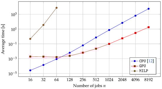
Figure 5. Computation time required to solve CAP instances using different algorithms.

To improve the performance, a hot-starting method was also tested. High-quality solutions were generated using the one-opt heuristic [12]. Unfortunately, the hot-start had no impact on the computation time, as the technique is generally more effective when finding feasible solutions is hard. Providing a lower bound, analogous to (24), also did not affect the computation time.

The sequential [12] algorithm and the new parallel one were able to solve all the considered instances. The parallel algorithm was inferior in respect to the sequential one for $n<128$, mostly due to an overhead of using GPU. For larger instances, the speedup was increasing steadily, reaching almost 314 for $n=8192$ (see Figure 6). While in the considered bicycle factory the number of jobs usually does not exceed 400, the ability to schedule larger payloads might be important in different applications, e.g., where welding time is shorter. However, even for $n=256$ the speedup obtained is significant, allowing to assign jobs in almost 10 times more product mixtures or processing orders in the same time (i.e., solve 10 times more problem instances).

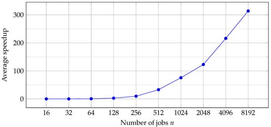
Figure 6. Speedup of the parallel algorithm executed on GPU, in relation to the sequential algorithm executed on a single CPU thread.

8. Concluding Remarks

The paper considered Cyclic Assignment Problem (CAP) in a two machine robotic cell, the problem inspired by a bicycle frame welding station. Two solving methods were introduced: One based on a Mixed Integer Linear Programming (MILP) model and a dedicated parallel algorithm. The algorithm was designed to benefit from a large number of processors, available, e.g. in modern GPUs. The proposed method efficiently transforms CAP into All Pairs Shortest Path (APSP) problem, allowing the user to utilize a vast literature on shortest path problems. The algorithm was analyzed theoretically, showing the computational complexity of up to $O(logn+T_{\mathrm{APSP}})$, where n is the size of the problem and $T_{\mathrm{APSP}}$ is the computational complexity of the APSP solving method used. For a well-known, parallel APSP solving algorithm, the overall computational complexity of the proposed algorithm is $O\left({log}^{2}n\right)$ on $n^3$-processor Exclusive Read Exclusive Write Parallel Random-Access Machine (EREW PRAM).

The computational experiments shown CAP to be relatively hard for the solver-based approach. MILP formulation, solved by Gurobi Optimizer, performed much worse than the dedicated methods. The solver was unable to find any optimal solutions for instances with $n\ge 128$ jobs in 2 h, while the dedicated algorithms solved the instances with $n=128$ in milliseconds. For the smaller instances, the solver was from ${10}^4$ to ${10}^7$ times slower on average than the sequential algorithm. The proposed parallel algorithm executed on a Graphics Processing Unit (GPU) was shown to achieve up to 314 speedup, compared to a sequential, state of art algorithm executed on CPU. The new method scheduled instances consisting of 8192 jobs in under 18 s and can be used both to solve larger instances and to shorten the computations for medium-sized ones. In practice, it allows to quickly re-assign the machines on the fly, when the demand changes. Alternatively, when the order of jobs is also to be determined, more potential orders can be evaluated by quickly finding the optimal assignments for each one (e.g., within a two-level metaheuristics described in Section 1).

A promising direction for future work is to address robotic cells with more than $m=2$ machines. While a very large m might be unrealistic (only a single machine processes jobs at any time; the remaining ones are idle), a moderate values $2<m<11$ can model various specialized pieces of equipment available at the workstation. Another interesting direction is to research compound problems, where CAP is a part of a larger production environment, similar to the one considered in [12].

References

- Allahverdi, A. The third comprehensive survey on scheduling problems with setup times/costs. Eur. J. Oper. Res. 2015, 246, 345–378. [Google Scholar] [CrossRef]
- Allahverdi, A. A survey of scheduling problems with no-wait in process. Eur. J. Oper. Res. 2016, 255, 665–686. [Google Scholar] [CrossRef]
- Chaudhry, I.A.; Khan, A.A. A research survey: Review of flexible job shop scheduling techniques. Int. Trans. Oper. Res. 2016, 23, 551–591. [Google Scholar] [CrossRef]
- Vlk, M.; Novak, A.; Hanzalek, Z.; Malapert, A. Non-overlapping Sequence-Dependent Setup Scheduling with Dedicated Tasks. In International Conference on Operations Research and Enterprise Systems; Springer: Berlin/Heidelberg, Germany, 2019; pp. 23–46. [Google Scholar] [CrossRef]
- Halim, A.H.; Ismail, I. Combinatorial optimization: Comparison of heuristic algorithms in travelling salesman problem. Arch. Comput. Methods Eng. 2019, 26, 367–380. [Google Scholar] [CrossRef]
- Lust, T.; Teghem, J. The multiobjective multidimensional knapsack problem: A survey and a new approach. Int. Trans. Oper. Res. 2012, 19, 495–520. [Google Scholar] [CrossRef]
- Gansterer, M.; Hartl, R.F. Collaborative vehicle routing: A survey. Eur. J. Oper. Res. 2018, 268, 1–12. [Google Scholar] [CrossRef]
- Montoya-Torres, J.R.; López Franco, J.; Nieto Isaza, S.; Felizzola Jiménez, H.; Herazo-Padilla, N. A literature review on the vehicle routing problem with multiple depots. Comput. Ind. Eng. 2015, 79, 115–129. [Google Scholar] [CrossRef]
- Lei, D.; Li, M.; Wang, L. A Two-Phase Meta-Heuristic for Multiobjective Flexible Job Shop Scheduling Problem With Total Energy Consumption Threshold. IEEE Trans. Cybern. 2019, 49, 1097–1109. [Google Scholar] [CrossRef] [PubMed]
- Zhang, F.; Mei, Y.; Zhang, M. A Two-Stage Genetic Programming Hyper-Heuristic Approach with Feature Selection for Dynamic Flexible Job Shop Scheduling. In Proceedings of the Genetic and Evolutionary Computation Conference, Prague, Czech Republic, 13–17 July 2019; Association for Computing Machinery: New York, NY, USA, 2019; pp. 347–355. [Google Scholar] [CrossRef]
- Aringhieri, R.; Landa, P.; Soriano, P.; Tànfani, E.; Testi, A. A two level metaheuristic for the operating room scheduling and assignment problem. Comput. Oper. Res. 2015, 54, 21–34. [Google Scholar] [CrossRef]
- Bożejko, W.; Gnatowski, A.; Idzikowski, R.; Wodecki, M. Cyclic flow shop scheduling problem with two-machine cells. Arch. Control Sci. 2017, 27, 151–167. [Google Scholar] [CrossRef][Green Version]
- Maniezzo, V.; Boschetti, M.A.; Stützle, T. Very Large-Scale Neighborhood Search. In Matheuristics: Algorithms and Implementations; Springer International Publishing: Cham, Switzerland, 2021; pp. 143–158. [Google Scholar] [CrossRef]
- Ahuja, R.K.; Özlem, E.; Orlin, J.B.; Punnen, A.P. A survey of very large-scale neighborhood search techniques. Discret. Appl. Math. 2002, 123, 75–102. [Google Scholar] [CrossRef]
- Gultekin, H.; Akturk, M.S.; Karasan, O.E. Cyclic scheduling of a 2-machine robotic cell with tooling constraints. Eur. J. Oper. Res. 2006, 174, 777–796. [Google Scholar] [CrossRef][Green Version]
- Majumder, A.; Laha, D. A new cuckoo search algorithm for 2-machine robotic cell scheduling problem with sequence-dependent setup times. Swarm Evol. Comput. 2016, 28, 131–143. [Google Scholar] [CrossRef]
- Gultekin, H.; Akturk, M.S.; Karasan, O.E. Scheduling in a three-machine robotic flexible manufacturing cell. Comput. Oper. Res. 2007, 34, 2463–2477. [Google Scholar] [CrossRef][Green Version]
- Marvel, J.A.; Bostelman, R.; Falco, J. Multi-Robot Assembly Strategies and Metrics. ACM Comput. Surv. 2018, 51, 1–32. [Google Scholar] [CrossRef]
- Mutti, S.; Nicola, G.; Beschi, M.; Pedrocchi, N.; Tosatti, L.M. Towards optimal task positioning in multi-robot cells, using nested meta-heuristic swarm algorithms. Robot. Comput. Integr. Manuf. 2021, 71, 102131. [Google Scholar] [CrossRef]
- Gultekin, H.; Coban, B.; Akhlaghi, V.E. Cyclic scheduling of parts and robot moves in m -machine robotic cells. Comput. Oper. Res. 2018, 90, 161–172. [Google Scholar] [CrossRef]
- Al-Ahmari, A. Optimal robotic cell scheduling with controllers using mathematically based timed Petri nets. Inf. Sci. 2016, 329, 638–648. [Google Scholar] [CrossRef]
- Ou, X.; Chang, Q.; Chakraborty, N. Simulation study on reward function of reinforcement learning in gantry work cell scheduling. J. Manuf. Syst. 2019, 50, 1–8. [Google Scholar] [CrossRef]
- Ou, X.; Chang, Q.; Chakraborty, N. A method integrating Q-Learning with approximate dynamic programming for gantry work cell scheduling. IEEE Trans. Autom. Sci. Eng. 2020, 18, 85–93. [Google Scholar] [CrossRef]
- Kampmeyer, T. Cyclic Scheduling Problems. Ph.D. Thesis, University of Osnabruck, Osnabruck, Germany, 2006. [Google Scholar]
- Levner, E.; Kats, V.; De Pablo, D.A.L.; Cheng, T.E. Complexity of cyclic scheduling problems: A state-of-the-art survey. Comput. Ind. Eng. 2010, 59, 352–361. [Google Scholar] [CrossRef]
- Yadav, A.; Jayswal, S. Modelling of flexible manufacturing system: A review. Int. J. Prod. Res. 2018, 56, 2464–2487. [Google Scholar] [CrossRef]
- Lee, T.; Loong, Y. A review of scheduling problem and resolution methods in flexible flow shop. Int. J. Ind. Eng. Comput. 2019, 10, 67–88. [Google Scholar] [CrossRef]
- Li, X.; Gao, L. Review for Flexible Job Shop Scheduling. In Effective Methods for Integrated Process Planning and Scheduling; Springer: Berlin/Heidelberg, Germany, 2020; pp. 17–45. [Google Scholar] [CrossRef]
- Gao, K.; Cao, Z.; Zhang, L.; Chen, Z.; Han, Y.; Pan, Q. A review on swarm intelligence and evolutionary algorithms for solving flexible job shop scheduling problems. IEEE/CAA J. Autom. Sin. 2019, 6, 904–916. [Google Scholar] [CrossRef]
- Ghadiri Nejad, M.; Kovács, G.; Vizvári, B.; Barenji, R.V. An optimization model for cyclic scheduling problem in flexible robotic cells. Int. J. Adv. Manuf. Technol. 2018, 95, 3863–3873. [Google Scholar] [CrossRef]
- Burcin Ozsoydan, F.; Sağir, M. Iterated greedy algorithms enhanced by hyper-heuristic based learning for hybrid flexible flowshop scheduling problem with sequence dependent setup times: A case study at a manufacturing plant. Comput. Oper. Res. 2021, 125, 105044. [Google Scholar] [CrossRef]
- Nawaz, M.; Enscore, E.E.; Ham, I. A heuristic algorithm for the m-machine, n-job flow-shop sequencing problem. Omega 1983, 11, 91–95. [Google Scholar] [CrossRef]
- Kress, D.; Müller, D.; Nossack, J. A worker constrained flexible job shop scheduling problem with sequence-dependent setup times. OR Spectrum 2019, 41, 179–217. [Google Scholar] [CrossRef]
- Chen, Z.L. Simultaneous job scheduling and resource allocation on parallel machines. Ann. Oper. Res. 2004, 129, 135–153. [Google Scholar] [CrossRef]
- Shabtay, D.; Steiner, G. A survey of scheduling with controllable processing times. Discret. Appl. Math. 2007, 155, 1643–1666. [Google Scholar] [CrossRef]
- Daniels, R.L.; Mazzola, J.B. Flow shop scheduling with resource flexibility. Oper. Res. 1994, 42, 504–522. [Google Scholar] [CrossRef]
- Hsieh, P.H.; Yang, S.J.; Yang, D.L. Decision support for unrelated parallel machine scheduling with discrete controllable processing times. Appl. Soft Comput. 2015, 30, 475–483. [Google Scholar] [CrossRef]
- Ruiz, R.; Andrés-Romano, C. Scheduling unrelated parallel machines with resource-assignable sequence-dependent setup times. Int. J. Adv. Manuf. Technol. 2011, 57, 777–794. [Google Scholar] [CrossRef]
- Okubo, H.; Miyamoto, T.; Yoshida, S.; Mori, K.; Kitamura, S.; Izui, Y. Project scheduling under partially renewable resources and resource consumption during setup operations. Comput. Ind. Eng. 2015, 83, 91–99. [Google Scholar] [CrossRef]
- Tempelmeier, H.; Buschkühl, L. Dynamic multi-machine lotsizing and sequencing with simultaneous scheduling of a common setup resource. Int. J. Prod. Econ. 2008, 113, 401–412. [Google Scholar] [CrossRef]
- Gnatowski, A.; Rudy, J.; Idzikowski, R. On two-machine Flow Shop Scheduling Problem with disjoint setups. In Proceedings of the 2020 IEEE 15th International Conference of System of Systems Engineering (SoSE), Budapest, Hungary, 2–4 June 2020; pp. 277–282. [Google Scholar] [CrossRef]
- Blelloch, G.E. Programming parallel algorithms. Commun. ACM 1996, 39, 85–97. [Google Scholar] [CrossRef]
- Fortune, S.; Wyllie, J. Parallelism in random access machines. In Proceedings of the Tenth annual ACM Symposium on Theory of Computing—STOC ’78, San Diego, CA, USA, 1–3 May 1978; ACM Press: New York, NY, USA, 1978; pp. 114–118. [Google Scholar] [CrossRef]
- Goldschlager, L.M. A unified approach to models of synchronous parallel machines. In Proceedings of the Tenth Annual ACM Symposium on Theory of Computing—STOC ’78, San Diego, CA, USA, 1–3 May 1978; ACM Press: New York, NY, USA, 1978; pp. 89–94. [Google Scholar] [CrossRef]
- Skillicorn, D.B. Foundations of Parallel Programming; Cambridge International Series on Parallel Computation; Cambridge University Press: Cambridge, UK, 2005. [Google Scholar]
- Grama, A.; Gupta, A.; Karypis, G.; Kumar, V. Introduction to Parallel Computing, 2nd ed.; Addison-Wesley: Boston, MA, USA, 2003; p. 856. [Google Scholar]
- Ladner, R.E.; Fischer, M.J. Parallel Prefix Computation. J. ACM 1980, 27, 831–838. [Google Scholar] [CrossRef]
- Han, Y.; Reif, J. Efficient Parallel Algorithms for Computing All Pair Shortest Paths in Directed Graphs. Algorithmica 1997, 17, 399–415. [Google Scholar] [CrossRef][Green Version]
- Meyer, U.; Sanders, P. Δ-stepping: A parallelizable shortest path algorithm. J. Algorithms 2003, 49, 114–152. [Google Scholar] [CrossRef]
- Lund, B.; Smith, J.W. A Multi-Stage CUDA Kernel for Floyd-Warshall. arXiv 2010, arXiv:1001.4108v2. [Google Scholar]
Publisher’s Note: MDPI stays neutral with regard to jurisdictional claims in published maps and institutional affiliations. |
© 2021 by the authors. Licensee MDPI, Basel, Switzerland. This article is an open access article distributed under the terms and conditions of the Creative Commons Attribution (CC BY) license (https://creativecommons.org/licenses/by/4.0/).