Low-Complexity Alternatives to the Optimal Linear Coding Scheme for Transmitting ARMA Sources

Abstract

In the era of the Internet of Things, there are many applications where numerous devices are deployed to acquire information and send it to analyse the data and make informed decisions. In these applications, the power consumption and price of the devices are often an issue. In this work, analog coding schemes are considered, so that an ADC is not needed, allowing the size and power consumption of the devices to be reduced. In addition, linear and DFT-based transmission schemes are proposed, so that the complexity of the operations involved is lowered, thus reducing the requirements in terms of processing capacity and the price of the hardware. The proposed schemes are proved to be asymptotically optimal among the linear ones for WSS, MA, AR and ARMA sources.

1. Introduction

In the past few years, and specially in the context of the Internet of Things (IoT), numerous applications in which devices with constrained power and processing capacity acquire and transmit data have emerged. Therefore, it is crucial to find coding strategies for transmitting information with an acceptable distortion that are undemanding in terms of processing while minimizing power consumption. A well-known low-power and low-complexity coding strategy is the so called analog joint source-channel coding (see, e.g., [1]). In this context, some authors have lately proposed the use of low-power/low-cost all-analog sensors [2,3], avoiding the high power demanding analog-to-digital converters (ADC).

Here, we are focused on analog joint source-channel linear coding. Specifically, we study here the transmission of realizations of an n-dimensional continuous random vector over an additive white Gaussian noise (AWGN) channel employing a linear encoder and decoder. For this scenario, the minimum average transmission power under a fixed average distortion constraint is achieved whenever it is applied the coding strategy given by Lee and Petersen in [4]. Nevertheless, in [5,6] it was presented a linear coding scheme based on the discrete Fourier transform (DFT) that, with a lower complexity, is asymptotically optimal among the linear schemes in terms of transmission power for certain sources, namely wide-sense stationary (WSS) and asymptotically WSS (AWSS) autoregressive (AR) sources.

In this paper, we present two new DFT-based alternatives to the optimal linear coding scheme given in [4]. We prove that the average transmission power required for one of them is lower than for the approach in [5,6]. The average transmission power required for the other new alternative is shown to be higher, although it is conceptually simpler, and so is its implementation. We prove that the two new schemes along with the strategy in [5,6] are asymptotically optimal for any AWSS source. Additionally, we show that the convergence speed of the average transmission power of the alternative schemes is $O(1/\sqrt{n})$ for the case of WSS, moving average (MA), AWSS AR and AWSS autoregressive moving average (ARMA) sources. Therefore, we conclude that it is possible to achieve a good performance with small size data blocks, allowing this schemes to be used in applications that require low latency.

This paper is organized as follows. In Section 2, we mathematically describe the communications system and review the transmission strategy presented in [4], and the alternative given in [5,6]. In Section 3, the two new coding schemes are presented. In Section 4, we compare the performance of each of the four coding strategies studied in terms of the required transmission power, and we analyze their asymptotic behavior for several types of sources. In Section 5 and Section 6 a numerical example and some conclusions are presented respectively.

2. Preliminaries

We begin this section by introducing some notation. We will denote by $\mathbb{R}$, $\mathbb{C}$, $\mathbb{Z}$ and $\mathbb{N}$ the sets of real numbers, complex numbers, integers and positive integers respectively. $\lceil a\rceil$ represents the smallest integer higher than or equal to $a\in \mathbb{R}$. ${\mathbb{R}}^{m\times n}$ is the set of the $m\times n$ real matrices. The symbols ⊤ and ∗ denote transpose and conjugate transpose respectively, the imaginary unit is represented by $\mathrm{i}$, $\mathrm{E}$ stands for expectation and $\delta$ is the Kronecker delta (i.e., ${\delta }_{j,k}=1$ if $j=k$, and it is zero otherwise). If $z\in \mathbb{C}$, $\mathrm{Re}\left(z\right)$ and $\mathrm{Im}\left(z\right)$ will designate the real part and the imaginary part of z respectively, $\overline{z}$ is the conjugate of z and $\widehat{z}$ is 2-dimensional the real column vector ${\left(\mathrm{Re}\left(z\right),\mathrm{Im}\left(z\right)\right)}^{\top }$. $I_n$ denotes the $n\times n$ identity matrix and $V_n$ is the $n\times n$ Fourier unitary matrix, i.e.,

$${\left[V_n\right]}_{j,k}=\frac{1}{\sqrt{n}}{\mathrm{e}}^{-\frac{2\pi (j-1)(k-1)}{n}\mathrm{i}}j,k\in \{1,\dots ,n\}.$$

${\lambda }_1\left(A\right),\dots ,{\lambda }_n\left(A\right)$ and ${\sigma }_1\left(B\right),\dots ,{\sigma }_n\left(B\right)$ are the eigenvalues of an $n\times n$ real symmetric matrix A and the singular values of an $n\times n$ matrix B sorted in decreasing order, respectively. If ${\left\{x_n\right\}}_{n\in \mathbb{N}}$ is a random process, we denote by $x_{n:1}$ the random n-dimensional column vector ${\left(x_n,x_{n-1},\dots ,x_1\right)}^{\top }$. The Frobenius norm and the spectral norm are represented by ${\parallel ·\parallel }_F$ and ${\parallel ·\parallel }_2$, respectively.

If $f:\mathbb{R}\to \mathbb{C}$ is a continuous and $2\pi$-periodic function, we denote by $T_n\left(f\right)$ the $n\times n$ Toeplitz matrix given by

$${\left[T_n\left(f\right)\right]}_{j,k}=f_{j-k},j,k\in \{1,\dots ,n\},$$

where ${\left\{f_k\right\}}_{k\in \mathbb{Z}}$ is the set of Fourier coefficients of f:

$$f_k=\frac{1}{2\pi }{\int }_0^{2\pi }f\left(\omega \right){\mathrm{e}}^{-k\omega \mathrm{i}}\mathrm{d}\omega \forall k\in \mathbb{Z}.$$

2.1. Problem Statement

We consider a discrete-time analog n-dimensional real vector source $x_{n:1}$ with invertible correlation matrix. We want to transmit realizations of this vector by using n times a real AWGN channel with noise variance ${\sigma }^2>0$. The n noise iid random variables can then be represented by the Gaussian n-dimensional vector ${\nu }_{n:1}$, with correlation matrix $\mathrm{E}\left({\nu }_{n:1}{\nu }_{n:1}^{\top }\right)={\sigma }^2{I}_n$. We further assume that the input $x_{n:1}$ and the channel noise ${\nu }_{n:1}$ are both zero-mean and that they are uncorrelated, i.e., $\mathrm{E}\left(x_j{\nu }_k\right)=0$ for all $j,k\in \{1,\dots ,n\}$.

The communications system is depicted in Figure 1, where G and H are $n\times n$ real matrices representing the linear encoder and decoder, respectively. Specifically, a source vector symbol is encoded using a linear transformation, $u_{n:1}=G{x}_{n:1}$, and then transmitted through the AWGN channel. An estimation of the source vector symbol is then obtained from the perturbed vector, $\widetilde{u_{n:1}}=u_{n:1}+{\nu }_{n:1}$, using another linear transformation, $\widetilde{x_{n:1}}=H\widetilde{u_{n:1}}$.

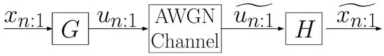
Figure 1. Linear coding scheme.

In [4], Lee and Petersen found matrices G and H that minimize the average transmission power, $\frac{1}{n}{\sum }_{j=1}^n\mathrm{E}(u_j^2)$, under a given average distortion constraint D, that is,

$$\frac{1}{n}\mathrm{E}\left({∥x_{n:1}-\widetilde{x_{n:1}}∥}_F^2\right)\le D.$$

2.2. Known Linear Coding Schemes

2.2.1. Optimal Linear Coding Scheme

As it has been aforementioned, Lee and Petersen presented the optimal linear coding scheme in [4]. The encoder of the optimal linear coding scheme converts the n correlated variables of the source vector into n uncorrelated variables, and assigns a weight to each of the n uncorrelated variables. If $\mathrm{E}\left(x_{n:1}{x}_{n:1}^{\top }\right)=U_n\mathrm{diag}({\lambda }_1\left(\mathrm{E}\left(x_{n:1}{x}_{n:1}^{\top }\right)\right),\dots ,$ ${\lambda }_n\left(\mathrm{E}\left(x_{n:1}{x}_{n:1}^{\top }\right)\right))U_n^{-1}$ is an eigenvalue decomposition of the correlation matrix of the source, where the eigenvector matrix $U_n$ is real and orthogonal, the optimal linear coding scheme is of the type shown in Figure 2, with $W_n=U_n^{\top }$. Its average transmission power is

$$P_n\left(D\right)=\frac{{\sigma }^2}{D}\left({\left(\frac{1}{n}{\displaystyle \sum _{j=1}^n}\sqrt{{\lambda }_j\left(\mathrm{E}\left(x_{n:1}{x}_{n:1}^{\top }\right)\right)}\right)}^2-D\right)$$

(1)

under a given average distortion constraint $D\in \left(0,{\lambda }_n\left(\mathrm{E}\left(x_{n:1}{x}_{n:1}^{\top }\right)\right)\right]$.

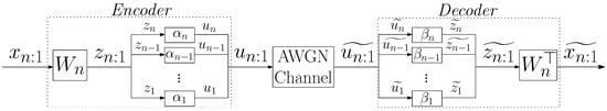
Figure 2. Linear coding scheme based on an $n\times n$ real orthogonal matrix $W_n$.

Since this coding scheme implies a multiplication of an $n\times n$ matrix by an $n\times 1$ column vector, its computational complexity is $O\left(n^2\right)$.

2.2.2. DFT-Based Alternative

In [5,6], an alternative to the optimal coding scheme was presented. The encoder of that alternative scheme assigns weights to the real and imaginary parts of the entries of the DFT of the source vector. This alternative coding scheme is of the type shown in Figure 2, with $W_n=M_n{V}_n^{*}$, where $M_n$ is the $n\times n$ sparse matrix defined in ([5] Equation (3)). Its average transmission power is

$${\widehat{P}}_n\left(D\right)=\frac{{\sigma }^2}{D}\left({\left(\frac{1}{n}{\displaystyle \sum _{j=1}^n}\sqrt{\mathrm{E}\left(z_j^2\right)}\right)}^2-D\right)$$

(2)

under a given average distortion constraint $D\in \left(0,{\lambda }_n\left(\mathrm{E}\left(x_{n:1}{x}_{n:1}^{\top }\right)\right)\right]$, where

$$\begin{array}{cc}\hfill & \mathrm{E}\left(z_{n-j+1}^2\right)=\left\{\begin{array}{cc}\mathrm{E}\left(y_{n-j+1}^2\right)\hfill & \mathrm{if}j\in \left\{1,\frac{n}{2}+1\right\}\cap \mathbb{N},\hfill \\ 2\mathrm{E}\left({\left(\mathrm{Re}\left(y_{n-j+1}\right)\right)}^2\right)\hfill & \mathrm{if}2\le j\le \lceil \frac{n}{2}\rceil ,\hfill \\ 2\mathrm{E}\left({\left(\mathrm{Im}\left(y_{n-j+1}\right)\right)}^2\right)\hfill & \mathrm{if}n-\lceil \frac{n}{2}\rceil +2\le j\le n,\hfill \end{array}\right.\hfill \end{array}$$

with $y_{n:1}=V_n^{*}{x}_{n:1}$.

The computational complexity of this coding scheme is $O(nlog(n\left)\right)$ whenever the fast Fourier transform (FFT) algorithm is used.

3. New Coding Schemes

In this section, we propose two new transmission schemes. Similarly to the scheme reviewed in Section 2.2.2, our two new schemes make use of the DFT, and their computational complexity is also $O(nlog(n\left)\right)$ if the FFT algorithm is applied.

3.1. Low-Power Alternative

The encoder of this scheme first computes the DFT of the source vector, $y_{n:1}=V_n^{*}{x}_{n:1}$. Afterwards, each 2-dimensional vector $\widehat{y_j}$ is encoded using a $2\times 2$ real orthogonal eigenvector matrix of the correlation matrix $\mathrm{E}\left(\widehat{y_j}{\widehat{y_j}}^{\top }\right)$. Therefore, the real part and the imaginary part of each $y_j$ are here jointly encoded, unlike in Section 2.2.2, where they where separately encoded. This coding scheme is shown in Figure 3 for n even (the scheme for n odd is similar), with

$$\mathrm{E}\left(\widehat{y_j}{\widehat{y_j}}^{\top }\right)=U_{\widehat{y_j}}\mathrm{diag}\left({\lambda }_1\left(\mathrm{E}\left(\widehat{y_j}{\widehat{y_j}}^{\top }\right)\right),{\lambda }_2\left(\mathrm{E}\left(\widehat{y_j}{\widehat{y_j}}^{\top }\right)\right)\right)U_{\widehat{y_j}}^{-1}\forall j\in \left\{⌈\frac{n+1}{2}⌉,\dots ,n-1\right\}$$

being an eigenvalue decomposition of $\mathrm{E}\left(\widehat{y_j}{\widehat{y_j}}^{\top }\right)$ where the eigenvector matrix $U_{\widehat{y_j}}$ is real and orthogonal,

$${\check{\alpha }}_j=\sqrt{\frac{1}{E(z_j^2)}\left(\sqrt{\frac{{\sigma }^2({\sigma }^2+{\check{P}}_n\left(D\right))E(z_j^2)}{D}}-{\sigma }^2\right)}\forall j\in \{1,\dots ,n\}$$

(3)

and

$${\check{\beta }}_j=\frac{{\check{\alpha }}_j\mathrm{E}\left(z_j^2\right)}{{\check{\alpha }}_j^2\mathrm{E}\left(z_j^2\right)+{\sigma }^2}\forall j\in \{1,\dots ,n\}.$$

(4)

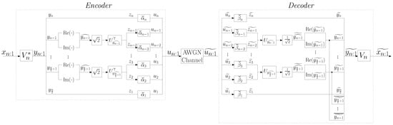
Figure 3. Low-power scheme.

In Appendix A, we prove that the average transmission power of this scheme under a given average distortion constraint D is

$${\check{P}}_n\left(D\right)=\frac{{\sigma }^2}{D}\left({\left(\frac{1}{n}{\displaystyle \sum _{j=1}^n}\sqrt{\mathrm{E}\left(z_j^2\right)}\right)}^2-D\right)\forall D\in \left(0,{\lambda }_n\left(\mathrm{E}\left(x_{n:1}{x}_{n:1}^{\top }\right)\right)\right],$$

(5)

with

$$\mathrm{E}\left(z_{n-j+1}^2\right)=\left\{\begin{array}{cc}\mathrm{E}\left(y_n^2\right)\hfill & \mathrm{if}j=1,\hfill \\ 2{\lambda }_1\left(\mathrm{E}\left(\widehat{y_{n-\frac{j}{2}}}{\widehat{y_{n-\frac{j}{2}}}}^{\top }\right)\right)\hfill & \mathrm{if}j\mathrm{even},j\ne n,\hfill \\ 2{\lambda }_2\left(\mathrm{E}\left(\widehat{y_{n-\frac{j-1}{2}}}{\widehat{y_{n-\frac{j-1}{2}}}}^{\top }\right)\right)\hfill & \mathrm{if}j\mathrm{odd},j\ne 1,\hfill \\ \mathrm{E}\left(y_{\frac{n}{2}}^2\right)\hfill & \mathrm{if}j=n,n\mathrm{even}.\hfill \end{array}\right.$$

Furthermore, in Section 4, we show that ${\check{P}}_n\left(D\right)\le {\widehat{P}}_n\left(D\right)$, i.e., the average transmission power for this new scheme is lower than the one required for the scheme in Section 2.2.2.

3.2. DFT/IDFT Alternative

The encoder of this scheme uses both the DFT and the inverse DFT (IDFT). The coding scheme is shown in Figure 4, where

$${\tilde{\alpha }}_j=\sqrt{\frac{1}{\mathrm{E}\left({\left|y_j\right|}^2\right)}\left(\sqrt{\frac{{\sigma }^2\left({\sigma }^2+{\tilde{P}}_n\left(D\right)\right)\mathrm{E}\left({\left|y_j\right|}^2\right)}{D}}-{\sigma }^2\right)}\forall j\in \{1,\dots ,n\}$$

(6)

and

$${\tilde{\beta }}_j=\frac{{\tilde{\alpha }}_j\mathrm{E}\left({\left|y_j\right|}^2\right)}{{\tilde{\alpha }}_j^2\mathrm{E}\left({\left|y_j\right|}^2\right)+{\sigma }^2}\forall j\in \{1,\dots ,n\}.$$

(7)

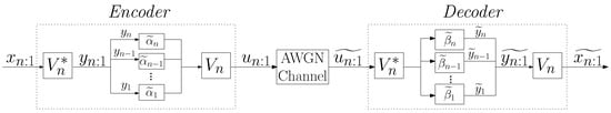
Figure 4. DFT/IDFT scheme.

In Appendix B, we prove that the average transmission power of this scheme under a given average distortion constraint D is

$${\tilde{P}}_n\left(D\right)=\frac{{\sigma }^2}{D}\left({\left(\frac{1}{n}{\displaystyle \sum _{j=1}^n}\sqrt{\mathrm{E}\left({\left|y_j\right|}^2\right)}\right)}^2-D\right)\forall D\in \left(0,{\lambda }_n\left(\mathrm{E}\left(x_{n:1}{x}_{n:1}^{\top }\right)\right)\right].$$

(8)

As it can be seen in Figure 4, this coding scheme is conceptually simpler than the ones in Section 2.2.2 and Section 3.1.

4. Analysis of the Transmission Power of the Coding Schemes

We begin this section by comparing the performance of each of the four considered coding strategies in terms of the required transmission power.

Theorem 1.

Let $P_n\left(D\right)$, ${\widehat{P}}_n\left(D\right)$, ${\check{P}}_n\left(D\right)$ and ${\tilde{P}}_n\left(D\right)$ be the average transmission powers given in (1), (2), (5) and (8), respectively. Then,

$$P_n\left(D\right)\le {\check{P}}_n\left(D\right)\le {\widehat{P}}_n\left(D\right)\le {\tilde{P}}_n\left(D\right).$$

(9)

Proof. 

See Appendix C. □

4.1. Asymptotic Behavior

We now show that the three alternatives to the optimal linear coding scheme, which were presented in Section 2.2.2, Section 3.1 and Section 3.2, are asymptotically optimal whenever the source is AWSS. To that end, we first need to review three definitions. We begin with the Gray concept of asymptotically equivalent sequences of matrices given in [7].

Definition 1

(Asymptotically equivalent sequences of matrices).Let $A_n$ and $B_n$ be $n\times n$ matrices for all $n\in \mathbb{N}$. The two sequences of matrices ${\left\{A_n\right\}}_{n\in \mathbb{N}}$ and ${\left\{B_n\right\}}_{n\in \mathbb{N}}$ are said to be asymptotically equivalent, abbreviated $\left\{A_n\right\}\sim \left\{B_n\right\}$, if there exists $M\ge 0$ such that

$$\parallel A_n{\parallel }_2,{\parallel B_n\parallel }_2\le M\forall n\in \mathbb{N}$$

and

$${\displaystyle \underset{n\to \infty }{lim}}\frac{\parallel A_n-B_n{\parallel }_F}{\sqrt{n}}=0.$$

Now we recall the well-known concept of WSS process.

Definition 2

(WSS process).Let $f:\mathbb{R}\to \mathbb{R}$ be a continuous, $2\pi$-periodic and non-negative function. A random process ${\left\{x_n\right\}}_{n\in \mathbb{N}}$ is said to be WSS, with power spectral density (PSD) f, if it has constant mean, i.e., $\mathrm{E}\left(x_j\right)=\mathrm{E}\left(x_k\right)\forall j,k\in \mathbb{N}$, and $\left\{\mathrm{E}\left(x_{n:1}{x}_{n:1}^{*}\right)\right\}=\left\{T_n\left(f\right)\right\}$.

We can now review the Gray concept of AWSS process given in ([8] p. 225).

Definition 3

(AWSS process).Let $f:\mathbb{R}\to \mathbb{R}$ be a continuous, $2\pi$-periodic and non-negative function. A random process ${\left\{x_n\right\}}_{n\in \mathbb{N}}$ is said to be AWSS, with (asymptotic) PSD f, if it has constant mean and $\left\{\mathrm{E}\left(x_{n:1}{x}_{x:1}^{*}\right)\right\}\sim \left\{T_n\left(f\right)\right\}$.

Theorem 2.

Suppose that ${\left\{x_n\right\}}_{n\in \mathbb{N}}$ is an AWSS process with PSD f as in Definition 3. If ${\displaystyle \underset{n\in \mathbb{N}}{inf}}{\lambda }_n\left(\mathrm{E}\left(x_{n:1}{x}_{n:1}^{\top }\right)\right)>0$ then

$${\displaystyle \underset{n\to \infty }{lim}}{P}_n\left(D\right)={\displaystyle \underset{n\to \infty }{lim}}{\widehat{P}}_n\left(D\right)={\displaystyle \underset{n\to \infty }{lim}}{\check{P}}_n\left(D\right)={\displaystyle \underset{n\to \infty }{lim}}{\tilde{P}}_n\left(D\right)=\frac{{\sigma }^2}{D}\left({\left(\frac{1}{2\pi }{\int }_0^{2\pi }\sqrt{f\left(\omega \right)}\mathrm{d}\omega \right)}^2-D\right)$$

for all $D\in \left(0,{\displaystyle \underset{n\in \mathbb{N}}{inf}}{\lambda }_n\left(\mathrm{E}\left(x_{n:1}{x}_{n:1}^{\top }\right)\right)\right]$.

Proof. 

See Appendix D. □

4.2. Convergence Speed

Here, we prove that the convergence speed of the average transmission power of the three alternative schemes described in Section 2.2.2, Section 3.1 and Section 3.2 to the average transmission power of the optimal linear scheme is $O(1/\sqrt{n})$ for AWSS ARMA, MA, AWSS AR and WSS sources. We also recall the definitions of ARMA, MA and AR processes.

4.2.1. AWSS ARMA Sources

Definition 4

(ARMA process).A real zero-mean random process ${\left\{x_n\right\}}_{n\in \mathbb{N}}$ is said to be ARMA if

$$x_n=w_n+{\displaystyle \sum _{j=1}^{n-1}}{b}_{-j}{w}_{n-j}-{\displaystyle \sum _{j=1}^{n-1}}{a}_{-j}{x}_{n-j}\forall n\in \mathbb{N},$$

(10)

where $b_{-j},a_{-j}\in \mathbb{R}$ for all $j\in \mathbb{N}$, and ${\left\{w_n\right\}}_{n\in \mathbb{N}}$ is a real zero-mean random process satisfying that $E\left(w_j{w}_k\right)={\delta }_{j,k}{\sigma }_w^2$ for all $j,k\in \mathbb{N}$ with ${\sigma }_w^2>0$. If there exist $p,q\in \mathbb{N}$ such that $a_{-j}=0$ for all $j>p$ and $b_{-j}=0$ for all $j>q$, then ${\left\{x_n\right\}}_{n\in \mathbb{N}}$ is called an ARMA$(p,q)$ process.

Theorem 3.

Suppose that ${\left\{x_n\right\}}_{n\in \mathbb{N}}$ is an ARMA($p,q$) process as in Definition 4. Let $a\left(\omega \right)=1+{\displaystyle {\displaystyle \sum _{j=1}^p}}{a}_{-j}{\mathrm{e}}^{-j\omega \mathrm{i}}$ and $b\left(\omega \right)=1+{\displaystyle {\displaystyle \sum _{j=1}^q}}{b}_{-j}{\mathrm{e}}^{-j\omega \mathrm{i}}$ for all $\omega \in \mathbb{R}$. Assume that $a\left(\omega \right)\ne 0$ and $b\left(\omega \right)\ne 0$ for all $\omega \in \mathbb{R}$, and that there exist $K_1,K_2>0$ such that ${∥{\left(T_n\left(a\right)\right)}^{-1}∥}_2\le K_1$ and ${∥{\left(T_n\left(b\right)\right)}^{-1}∥}_2\le K_2$ for all $n\in \mathbb{N}$. Then, ${\left\{x_n\right\}}_{n\in \mathbb{N}}$ is AWSS with PSD ${\sigma }_w^2\frac{{\left|b\right|}^2}{{\left|a\right|}^2}$, and

$${\tilde{P}}_n\left(D\right)-P_n\left(D\right)=O\left(1/\sqrt{n}\right).$$

(11)

for all $D\in \left(0,{\displaystyle \underset{n\in \mathbb{N}}{inf}}{\lambda }_n\left(\mathrm{E}\left(x_{n:1}{x}_{n:1}^{\top }\right)\right)\right]$.

Proof. 

See Appendix E. □

4.2.2. MA Sources

Definition 5

(MA process).A real zero-mean random process ${\left\{x_n\right\}}_{n\in \mathbb{N}}$ is said to be MA if

$$x_n=w_n+{\displaystyle \sum _{j=1}^{n-1}}{b}_{-j}{w}_{n-j}\forall n\in \mathbb{N},$$

where $b_{-j}\in \mathbb{R}$ for all $j\in \mathbb{N}$, and ${\left\{w_n\right\}}_{n\in \mathbb{N}}$ is a real zero-mean random process satisfying that $E\left(w_j{w}_k\right)={\delta }_{j,k}{\sigma }_w^2$ for all $j,k\in \mathbb{N}$ with ${\sigma }_w^2>0$. If there exists $q\in \mathbb{N}$ such that $b_{-j}=0$ for all $j>q$, then ${\left\{x_n\right\}}_{n\in \mathbb{N}}$ is called an MA$\left(q\right)$ process.

Theorem 4.

Suppose that ${\left\{x_n\right\}}_{n\in \mathbb{N}}$ is an MA(q) process as in Definition 5. Let $b\left(\omega \right)=1+{\displaystyle {\displaystyle \sum _{j=1}^q}}{b}_{-j}{\mathrm{e}}^{-j\omega \mathrm{i}}$ for all $\omega \in \mathbb{R}$. Assume that $b\left(\omega \right)\ne 0$ for all $\omega \in \mathbb{R}$, and that there exists $K>0$ such that ${∥{\left(T_n\left(b\right)\right)}^{-1}∥}_2\le K$ for all $n\in \mathbb{N}$. Then, ${\left\{x_n\right\}}_{n\in \mathbb{N}}$ is AWSS with PSD ${\sigma }_w^2{\left|b\right|}^2$, and

$${\tilde{P}}_n\left(D\right)-P_n\left(D\right)=O\left(1/\sqrt{n}\right).$$

for all $D\in \left(0,{\displaystyle \underset{n\in \mathbb{N}}{inf}}{\lambda }_n\left(\mathrm{E}\left(x_{n:1}{x}_{n:1}^{\top }\right)\right)\right]$.

Proof. 

It is a direct consequence of Theorem 3. □

4.2.3. AWSS AR Sources

Definition 6

(AR process).A real zero-mean random process ${\left\{x_n\right\}}_{n\in \mathbb{N}}$ is said to be AR if

$$x_n=w_n-{\displaystyle \sum _{j=1}^{n-1}}{a}_{-j}{x}_{n-j}\forall n\in \mathbb{N},$$

where $a_{-j}\in \mathbb{R}$ for all $j\in \mathbb{N}$, and ${\left\{w_n\right\}}_{n\in \mathbb{N}}$ is a real zero-mean random process satisfying that $E\left(w_j{w}_k\right)={\delta }_{j,k}{\sigma }_w^2$ for all $j,k\in \mathbb{N}$ with ${\sigma }_w^2>0$. If there exists $p\in \mathbb{N}$ such that $a_{-j}=0$ for all $j>p$, then ${\left\{x_n\right\}}_{n\in \mathbb{N}}$ is called an AR$\left(p\right)$ process.

Theorem 5.

Suppose that ${\left\{x_n\right\}}_{n\in \mathbb{N}}$ is an AR(p) process as in Definition 6. Let $a\left(\omega \right)=1+{\displaystyle {\displaystyle \sum _{j=1}^p}}{a}_{-j}{\mathrm{e}}^{-j\omega \mathrm{i}}$ for all $\omega \in \mathbb{R}$. Assume that $a\left(\omega \right)\ne 0$ for all $\omega \in \mathbb{R}$, and that there exists $K>0$ such that ${∥{\left(T_n\left(a\right)\right)}^{-1}∥}_2\le K$ for all $n\in \mathbb{N}$. Then, ${\left\{x_n\right\}}_{n\in \mathbb{N}}$ is AWSS with PSD $\frac{{\sigma }_w^2}{{\left|a\right|}^2}$, and

$${\tilde{P}}_n\left(D\right)-P_n\left(D\right)=O\left(1/\sqrt{n}\right).$$

for all $D\in \left(0,{\displaystyle \underset{n\in \mathbb{N}}{inf}}{\lambda }_n\left(\mathrm{E}\left(x_{n:1}{x}_{n:1}^{\top }\right)\right)\right]$.

Proof. 

It is a direct consequence of Theorem 3. □

4.2.4. WSS Sources

Theorem 6.

Suppose that ${\left\{x_n\right\}}_{n\in \mathbb{N}}$ is a WSS process as in Definition 2 with PSD f. Assume that $f\left(\omega \right)\ne 0$ for all $\omega \in \mathbb{R}$ and that there exists $m\in \mathbb{N}$ such that $f_k=0$ whenever $\left|k\right|>m$. Then,

$${\tilde{P}}_n\left(D\right)-P_n\left(D\right)=O\left(1/\sqrt{n}\right).$$

for all $D\in \left(0,min\left(f\right)\right]$.

Proof. 

See Appendix F. □

5. Numerical Example

In this section we give a numerical example. We consider an ARMA($1,1$) process ${\left\{x_n\right\}}_{n\in \mathbb{N}}$ with $a_{-1}=-\frac{1}{2}$, $b_{-1}=-\frac{1}{3}$ and ${\sigma }_w^2=1$, channel noise variance ${\sigma }^2=1$ and an average distortion constraint $D=0.5$. Figure 5 shows the theoretical value of the average transmission power required for each of the considered schemes with $n\in \{1,\dots ,100\}$. It can be observed how the graphs of the average transmission power of the different schemes follow the inequalities in (9), and how the transmission power of the different schemes get closer as n increases. Moreover, we have simulated the transmission of 20,000 samples of the considered ARMA($1,1$) process for $n\in \{1,\dots ,100\}$. Figure 6 shows the 10th and the 90th percentile of the power and distortion of the samples.

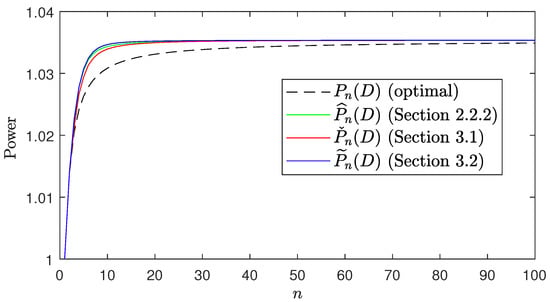
Figure 5. Theoretical average transmission powers of the considered schemes.

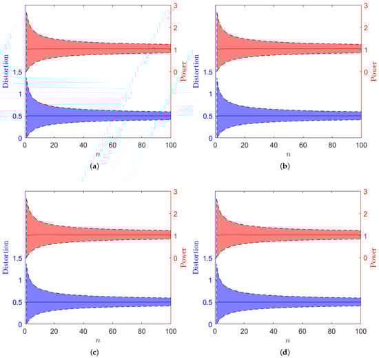
Figure 6. Interval between the 10th and the 90th percentile for the actual transmission power and the actual distortion (shaded) and theoretical average transmission power and distortion (solid line) in each of the considered schemes. (a) Optimal linear coding scheme (Section 2.2.1). (b) Low-power alternative (Section 3.1). (c) DFT-based alternative (Section 2.2.2). (d) DFT/IDFT alternative (Section 3.2).

6. Conclusions

In this paper, two new low-complexity linear coding schemes for transmitting n-dimensional vectors by using n times an AWGN channel have been presented. These schemes are based on the DFT. The performance of these schemes, along with another DFT-based scheme that had been previously presented, has been analyzed in comparison with the optimal scheme among the linear ones. These three DFT-based schemes allow good performance in terms of distortion using low-cost, low-power hardware.

In particular, it has been proved that, under a maximum average distortion constraint, the considered low-complexity schemes require the same average transmission power as the optimal linear scheme for AWSS sources when the block length, n, tends to infinity. Moreover, it has been proved that for certain types of AWSS sources (namely WSS, MA, AWSS AR and AWSS ARMA), the difference between the transmission power of each of the three alternative schemes and the transmission power of the optimal linear scheme decreases as $O\left(1/\sqrt{n}\right)$. Therefore, their performance will be similar to that of the optimal linear coding scheme even for small values of n. In other words, replacing the optimal linear scheme with any of the schemes studied here will not have, even for small block sizes, a large penalty in terms of transmission power, while it will lead to a noticeable reduction in complexity.

References

- Fresnedo, O.; Vazquez-Araujo, F.J.; Castedo, L.; Garcia-Frias, J. Low-Complexity Near-Optimal Decoding for Analog Joint Source Channel Coding Using Space-Filling Curves. IEEE Commun. Lett. 2013, 17, 745–748. [Google Scholar] [CrossRef]
- Sadhu, V.; Zhao, X.; Pompili, D. Energy-Efficient Analog Sensing for Large-Scale and High-Density Persistent Wireless Monitoring. IEEE Internet Things J. 2020, 7, 6778–6786. [Google Scholar] [CrossRef] [Green Version]
- Mouris, B.A.; Stavrou, P.A.; Thobaben, R. Optimizing Low-Complexity Analog Mappings for Low-Power Sensors with Energy Scheduling Capabilities. IEEE Internet Things J. 2022, 1. [Google Scholar] [CrossRef]
- Lee, K.H.; Petersen, D.P. Optimal Linear Coding for Vector Channels. IEEE Trans. Commun. 1976, 24, 1283–1290. [Google Scholar]
- Insausti, X.; Crespo, P.M.; Gutiérrez-Gutiérrez, J.; Zárraga-Rodríguez, M. Low-Complexity Analog Linear Coding Scheme. IEEE Commun. Lett. 2018, 22, 1754–1757. [Google Scholar] [CrossRef]
- Gutiérrez-Gutiérrez, J.; Villar-Rosety, F.M.; Zárraga-Rodríguez, M.; Insausti, X. A Low-Complexity Analog Linear Coding Scheme for Transmitting Asymptotically WSS AR Sources. IEEE Commun. Lett. 2019, 23, 773–776. [Google Scholar] [CrossRef]
- Gray, R.M. On the Asymptotic Eigenvalue Distribution of Toeplitz Matrices. IEEE Trans. Inf. Theory 1972, 18, 725–730. [Google Scholar] [CrossRef]
- Gray, R.M. Toeplitz and Circulant Matrices: A review. Found. Trends Commun. Inf. Theory 2006, 2, 155–239. [Google Scholar] [CrossRef]
- Gutiérrez-Gutiérrez, J.; Zárraga-Rodríguez, M.; Villar-Rosety, F.M.; Insausti, X. Rate-Distortion Function Upper Bounds for Gaussian Vectors and Their Applications in Coding AR Sources. Entropy 2018, 20, 399. [Google Scholar] [CrossRef] [PubMed] [Green Version]
- Gutiérrez-Gutiérrez, J.; Crespo, P.M. Block Toeplitz Matrices: Asymptotic Results and Applications. Found. Trends Commun. Inf. Theory 2011, 8, 179–257. [Google Scholar] [CrossRef] [Green Version]
- Zárraga-Rodríguez, M.; Gutiérrez-Gutiérrez, J.; Insausti, X. A Low-Complexity and Asymptotically Optimal Coding Strategy for Gaussian Vector Sources. Entropy 2019, 21, 965. [Google Scholar] [CrossRef] [Green Version]
- Gutiérrez-Gutiérrez, J.; Crespo, P.M. Asymptotically Equivalent Sequences of Matrices and Multivariate ARMA Processes. IEEE Trans. Inf. Theory 2011, 57, 5444–5454. [Google Scholar] [CrossRef]
- Gutiérrez-Gutiérrez, J.; Zárraga-Rodríguez, M.; Insausti, X. On the Asymptotic Optimality of a Low-Complexity Coding Strategy for WSS, MA, and AR Vector Sources. Entropy 2020, 22, 1378. [Google Scholar] [CrossRef] [PubMed]
Publisher’s Note: MDPI stays neutral with regard to jurisdictional claims in published maps and institutional affiliations. |
© 2022 by the authors. Licensee MDPI, Basel, Switzerland. This article is an open access article distributed under the terms and conditions of the Creative Commons Attribution (CC BY) license (https://creativecommons.org/licenses/by/4.0/).