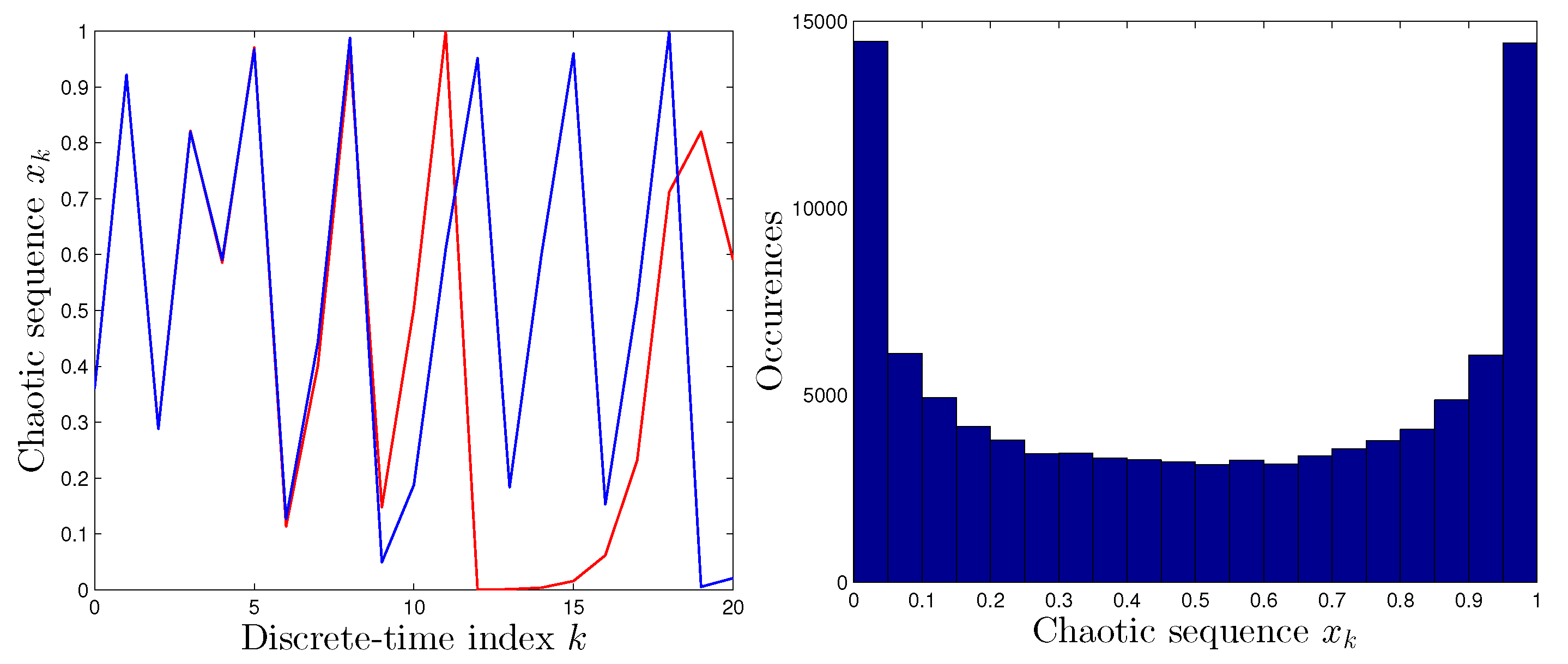
Figure 1.
Logistic map.
Left-hand panel: Comparison between system’s output with two different initial conditions. (The wave with initial value
is represented by the red line and the other with initial value
by the blue line.)
Right-hand panel: Occurrence histogram of the values of the states of the dynamical system (
1).
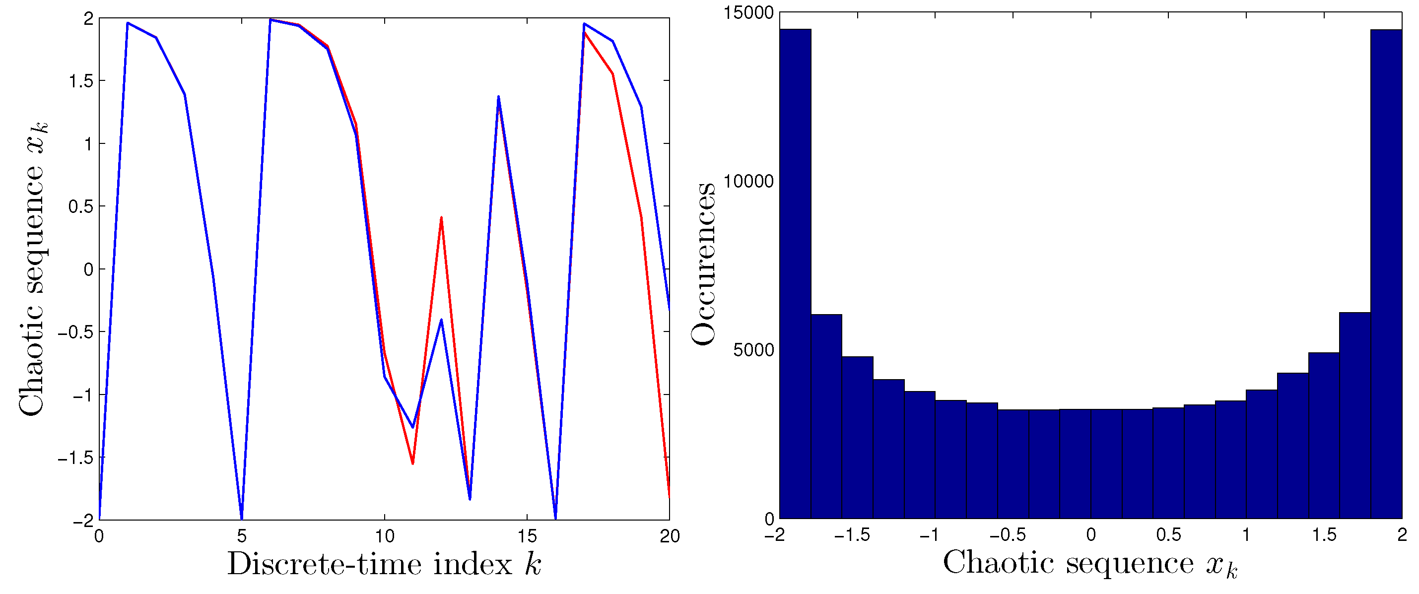
Figure 2.
Quadratic map.
Left-hand panel: Comparison between system’s output with two different, albeit very close, initial conditions.
Right-hand panel: Occurrence histogram of the values of the states of the dynamical system (
2).
Figure 2.
Quadratic map.
Left-hand panel: Comparison between system’s output with two different, albeit very close, initial conditions.
Right-hand panel: Occurrence histogram of the values of the states of the dynamical system (
2).
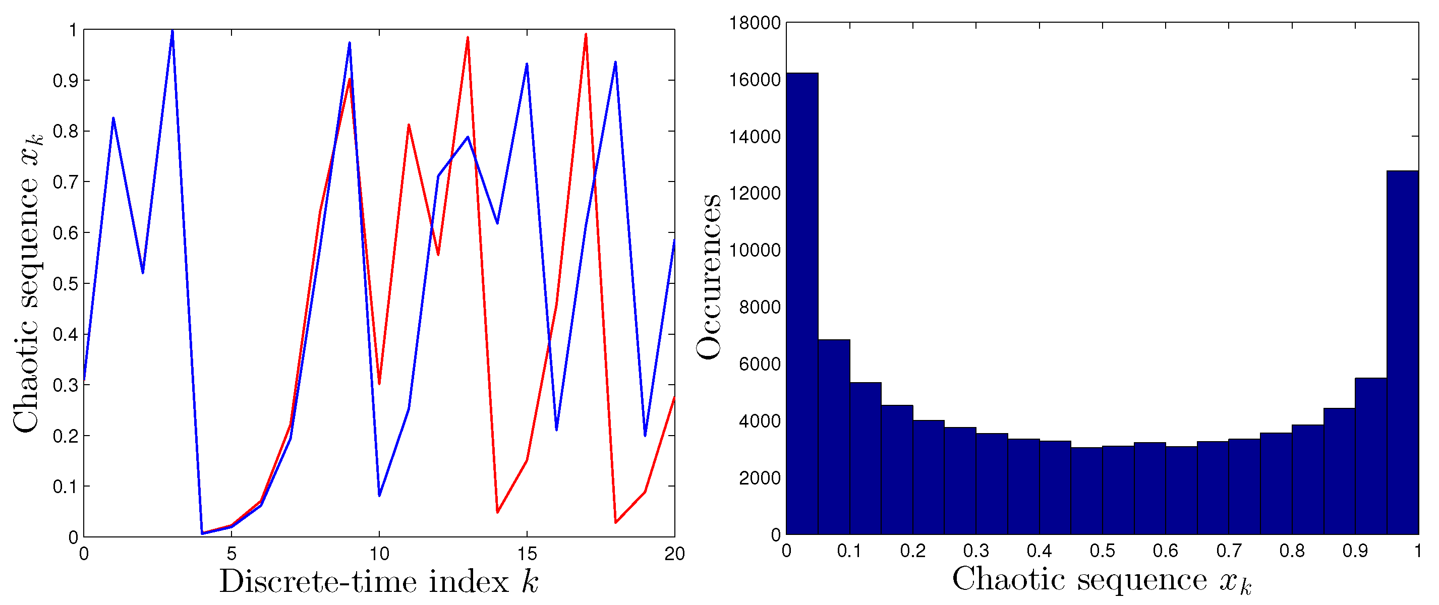
Figure 3.
Tent map.
Left-hand panel: Comparison between system’s output with two different, although very close, initial conditions.
Right-hand panel: Occurrence histogram of the values of the states of the dynamical system (
3).
Figure 3.
Tent map.
Left-hand panel: Comparison between system’s output with two different, although very close, initial conditions.
Right-hand panel: Occurrence histogram of the values of the states of the dynamical system (
3).
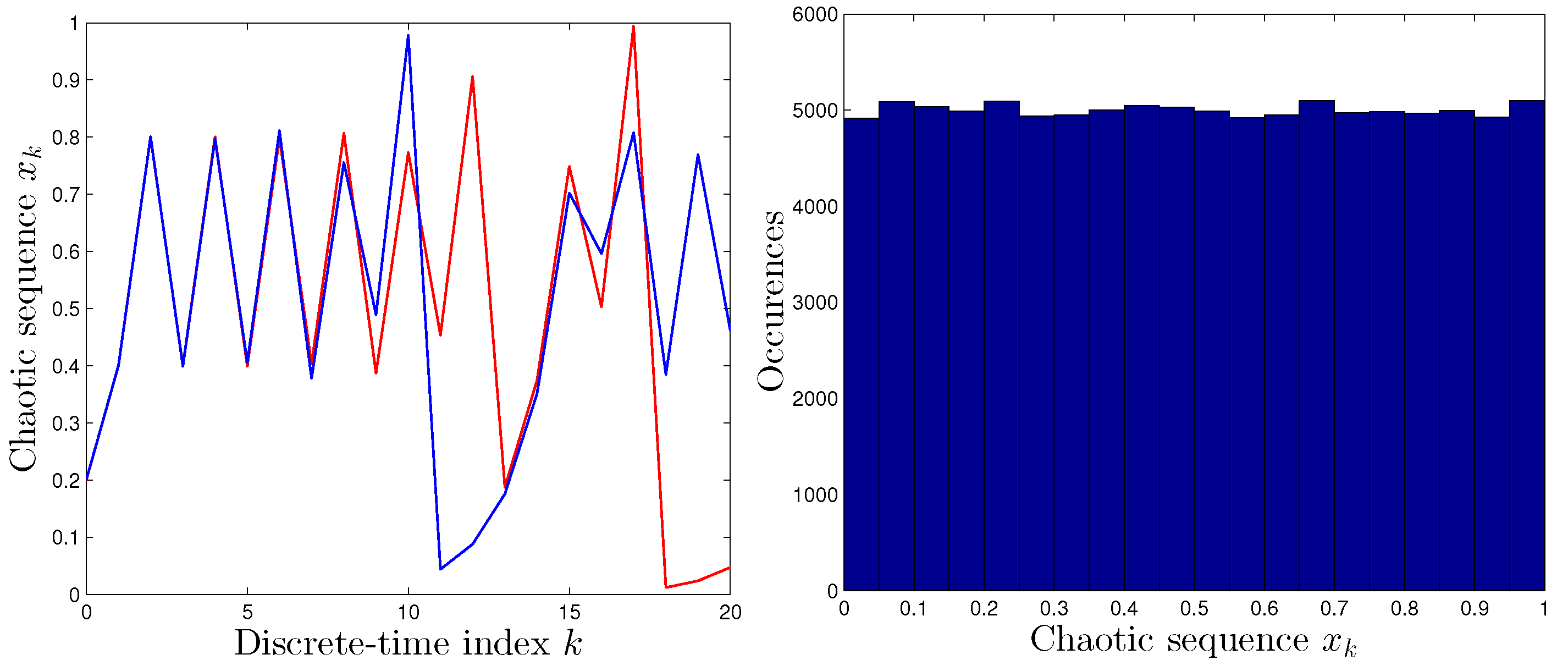
Figure 4.
Sine map.
Left-hand panel: Comparison between system’s output with two different initial conditions, very close to one another.
Right-hand panel: Occurrence histogram of the values of the states of the dynamical system (
4).
Figure 4.
Sine map.
Left-hand panel: Comparison between system’s output with two different initial conditions, very close to one another.
Right-hand panel: Occurrence histogram of the values of the states of the dynamical system (
4).
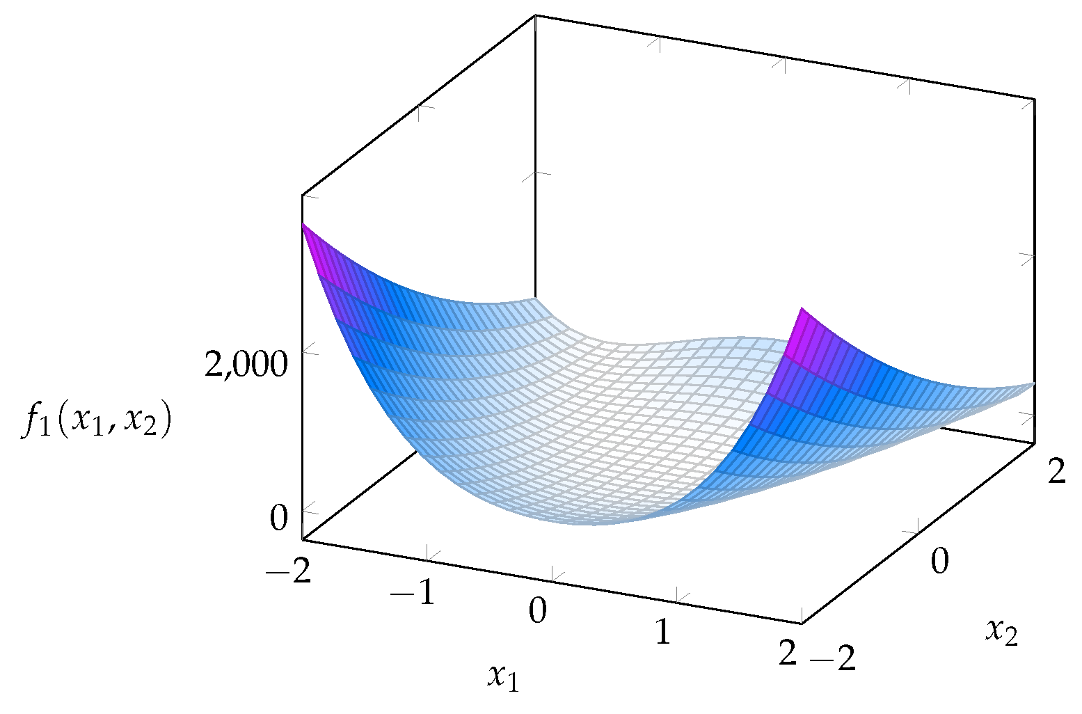
Figure 5.
Rendering of the generalized Rosenbrock function (benchmark function “F1”) for the case of independent variables.
Figure 5.
Rendering of the generalized Rosenbrock function (benchmark function “F1”) for the case of independent variables.
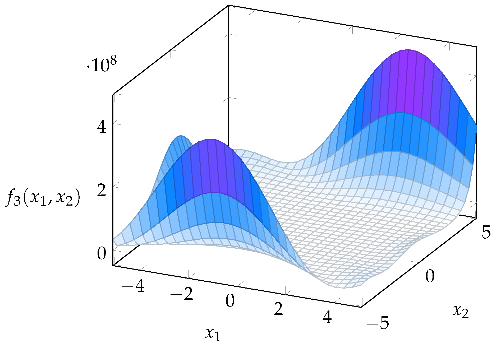
Figure 6.
Rendering of the Goldstein–Price function (benchmark function “F3”).
Figure 6.
Rendering of the Goldstein–Price function (benchmark function “F3”).
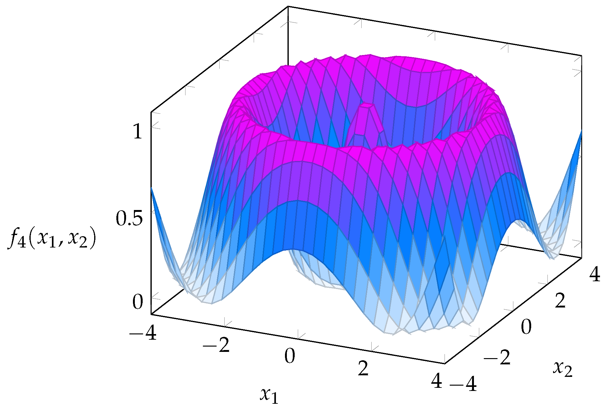
Figure 7.
Rendering of the Schaffer function (benchmark function “F4”).
Figure 7.
Rendering of the Schaffer function (benchmark function “F4”).
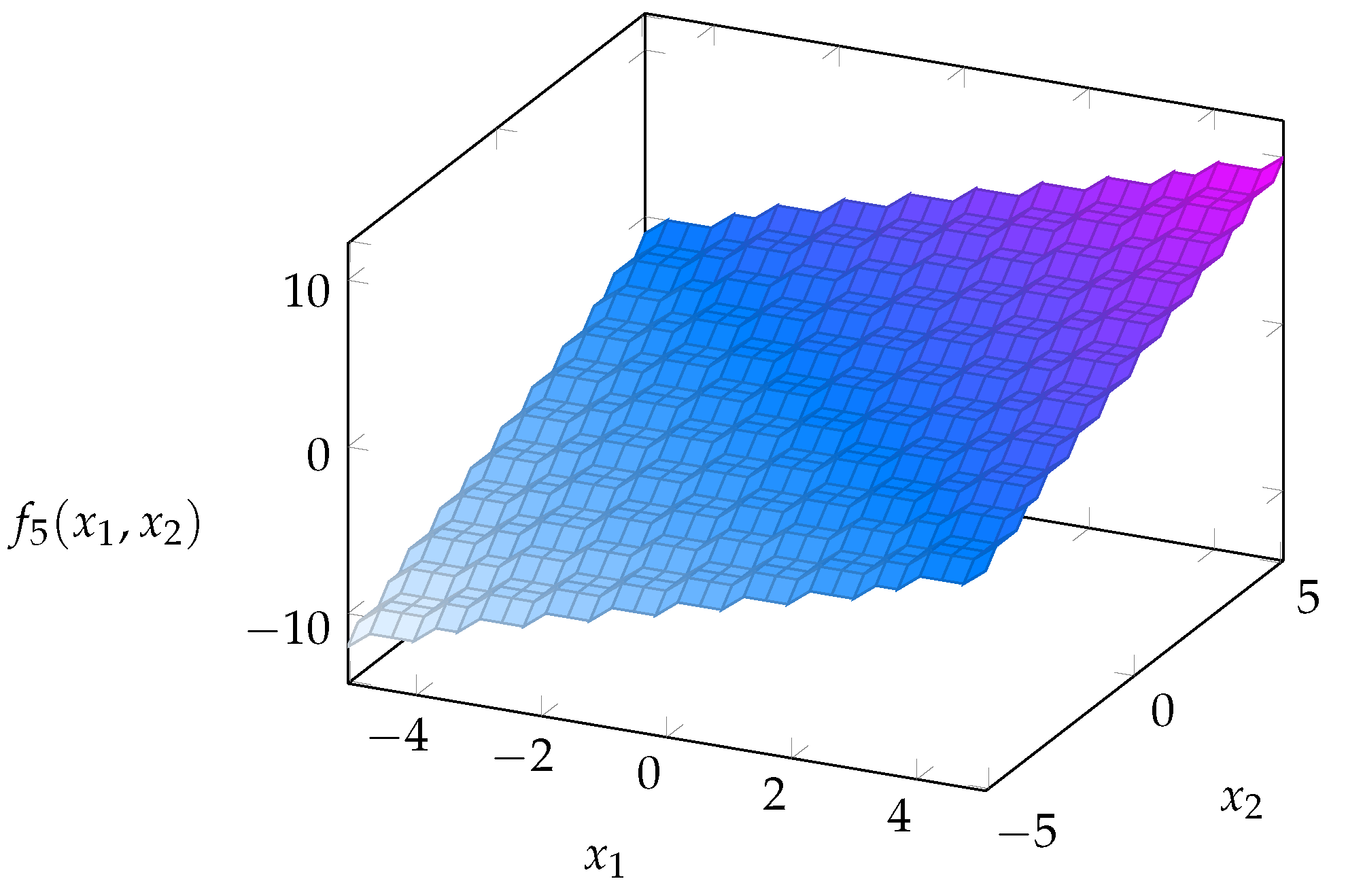
Figure 8.
Rendering of the “step” function (benchmark function “F5”) for the case of independent variables.
Figure 8.
Rendering of the “step” function (benchmark function “F5”) for the case of independent variables.
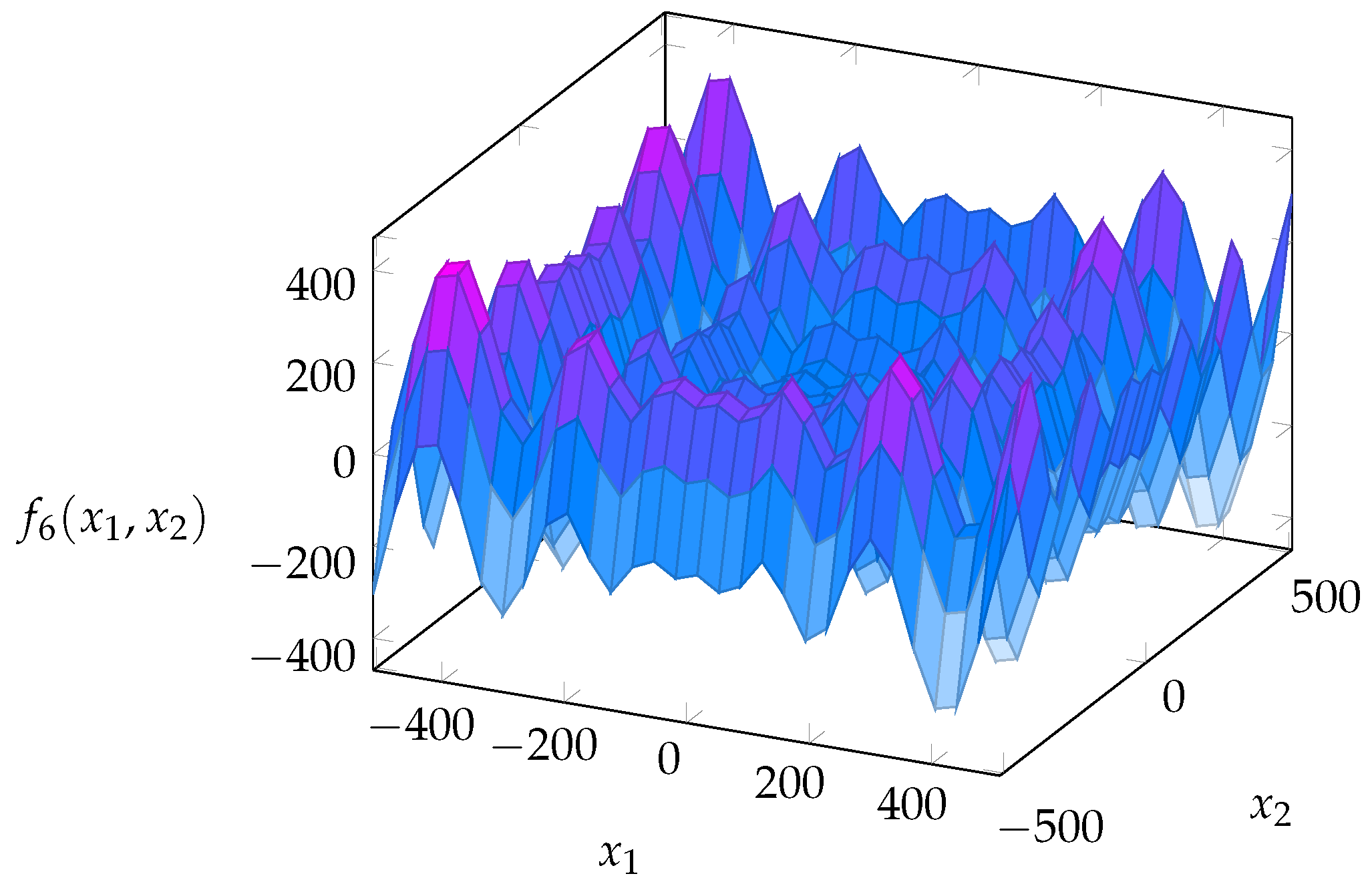
Figure 9.
Rendering of the Schwefel function (benchmark function “F6”) for the case of independent variables.
Figure 9.
Rendering of the Schwefel function (benchmark function “F6”) for the case of independent variables.
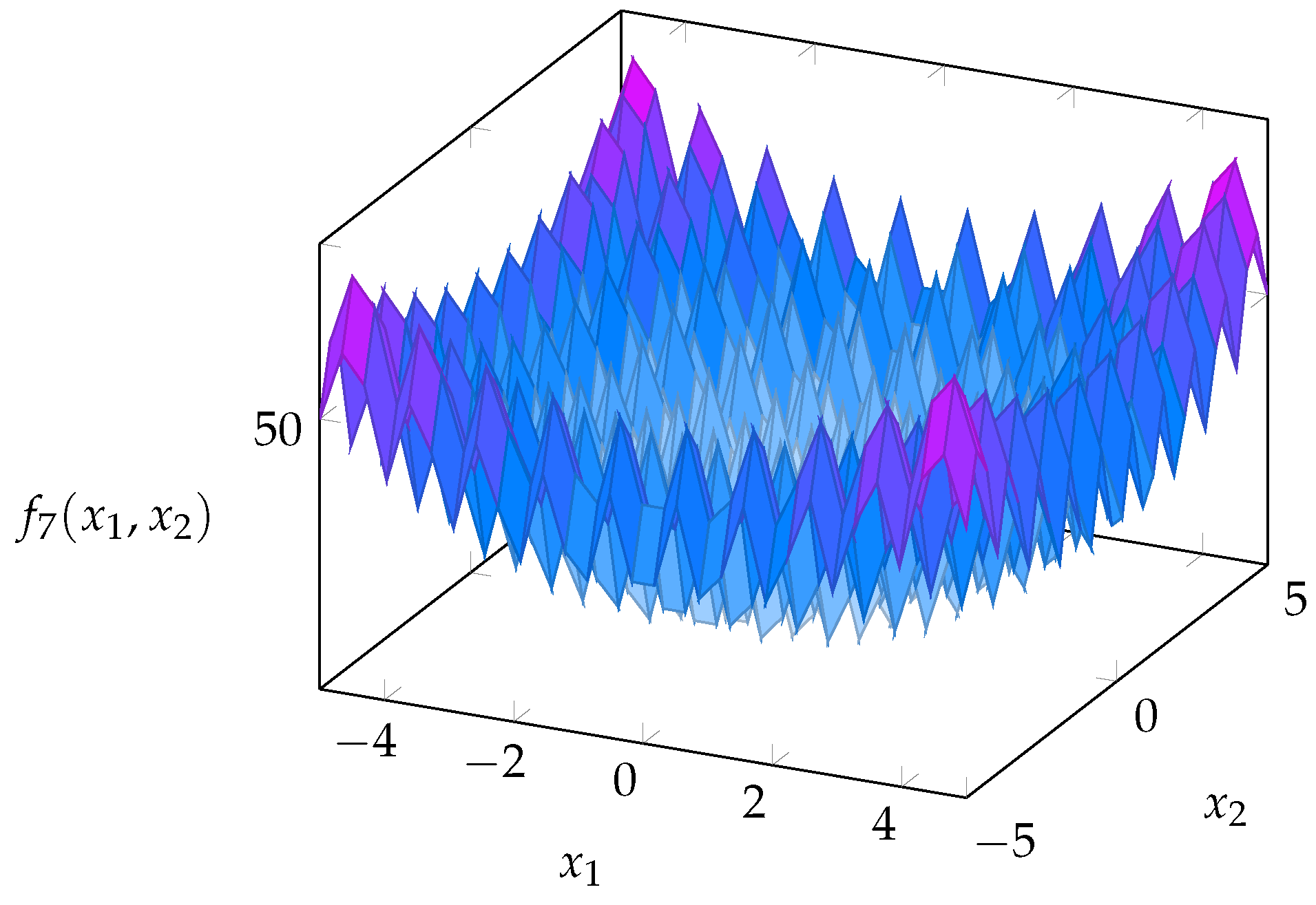
Figure 10.
Rendering of the Rastring function (benchmark function “F7”) for the case of independent variables.
Figure 10.
Rendering of the Rastring function (benchmark function “F7”) for the case of independent variables.
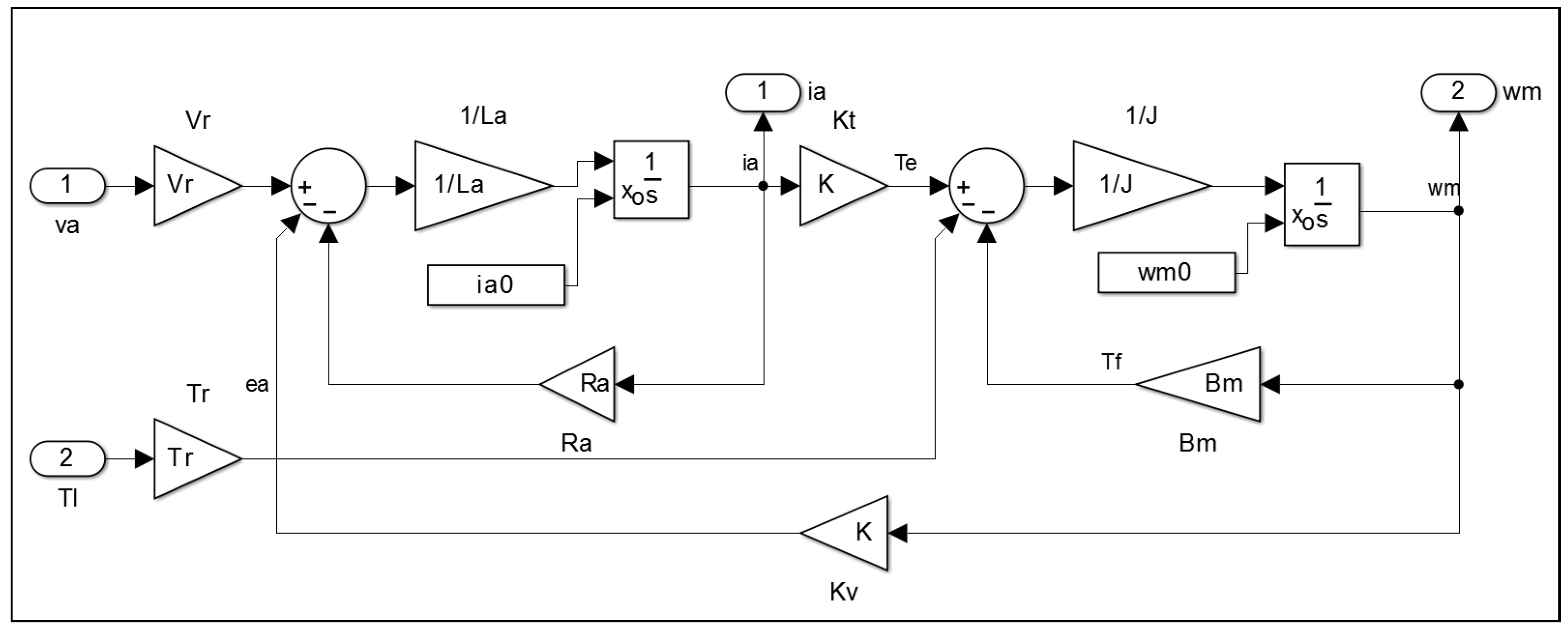
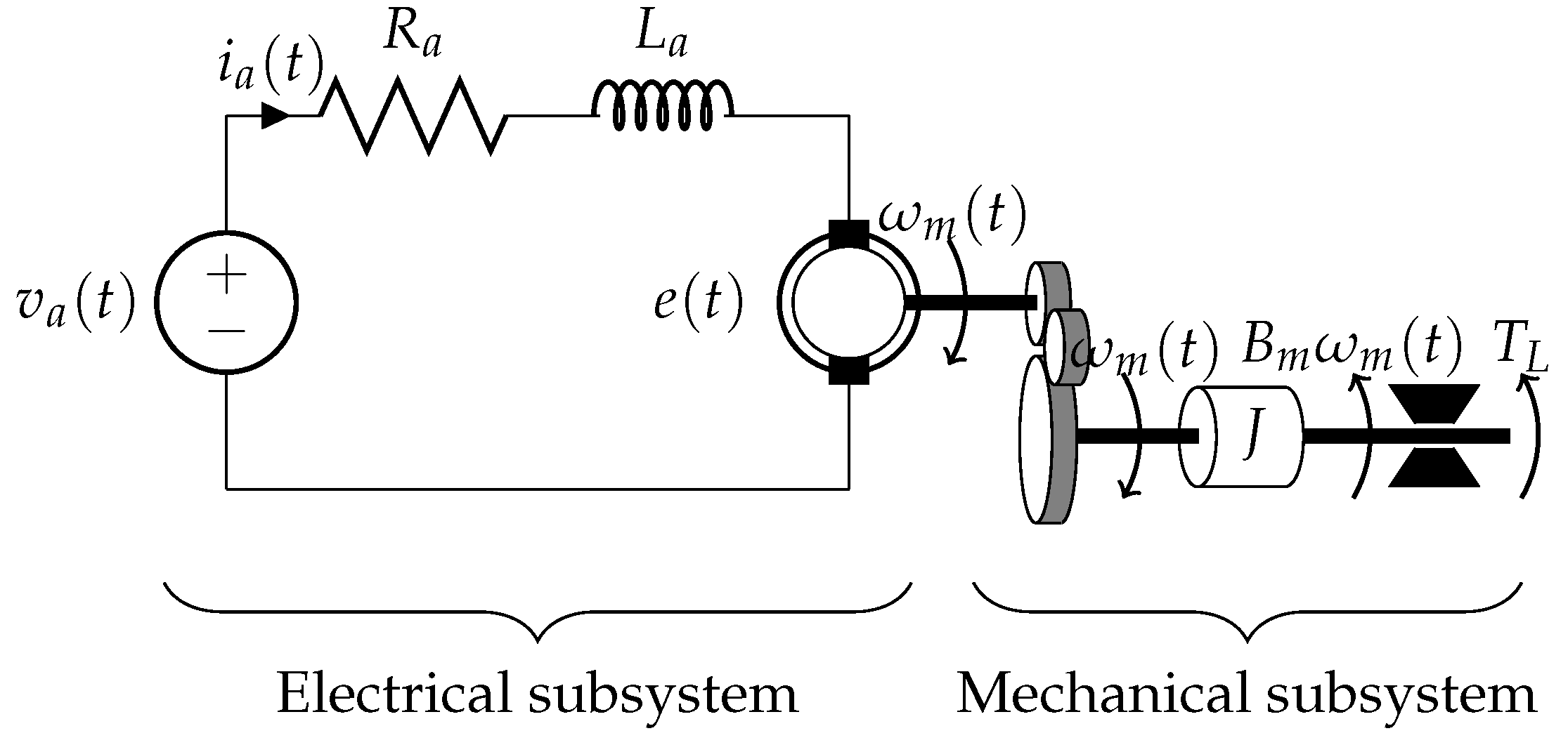
Figure 11.
An electro-mechanical model of the direct-current electrical motor (we assumed no angular speed change after gear).
Figure 11.
An electro-mechanical model of the direct-current electrical motor (we assumed no angular speed change after gear).
Figure 12.
A Simulink model of an electrical direct-current motor with constant stator voltage.
Figure 12.
A Simulink model of an electrical direct-current motor with constant stator voltage.
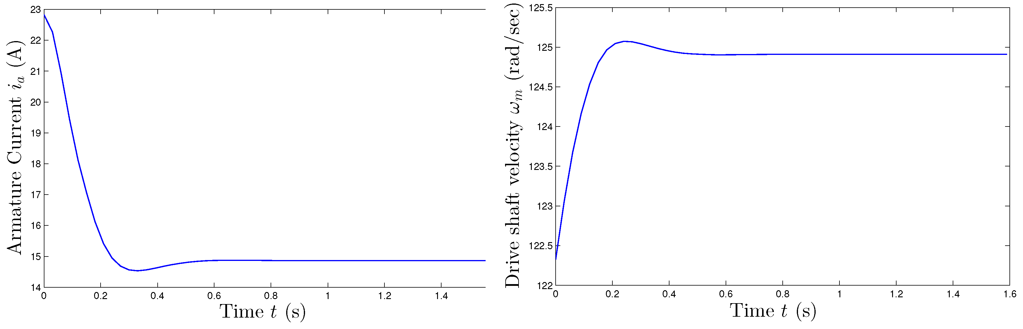
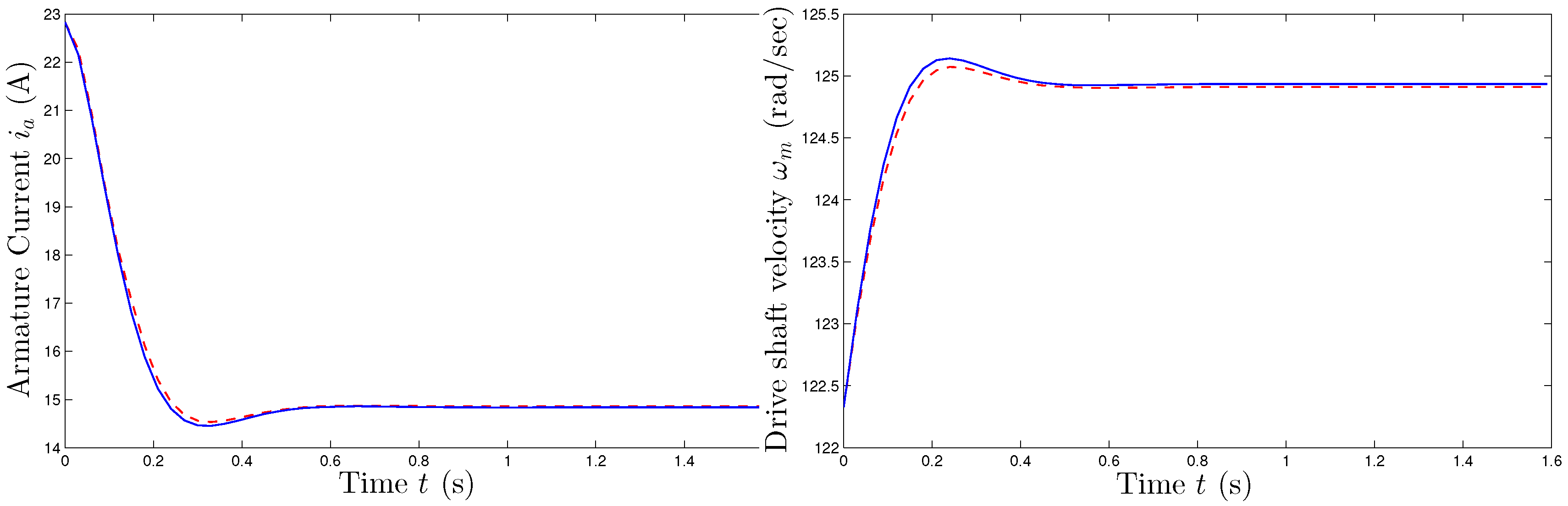
Figure 13.
Example of output values of the model of a direct-current electrical motor driven by a step input voltage. Left-hand panel: Armature current versus time. Right-hand panel: Drive shaft angular velocity versus time.
Figure 13.
Example of output values of the model of a direct-current electrical motor driven by a step input voltage. Left-hand panel: Armature current versus time. Right-hand panel: Drive shaft angular velocity versus time.
Figure 14.
Motor driven by a step armature voltage: Comparison of the output curves. Blue-solid line: Actual motor response. Red-crosshatched line: Inferred motor model response.
Figure 14.
Motor driven by a step armature voltage: Comparison of the output curves. Blue-solid line: Actual motor response. Red-crosshatched line: Inferred motor model response.
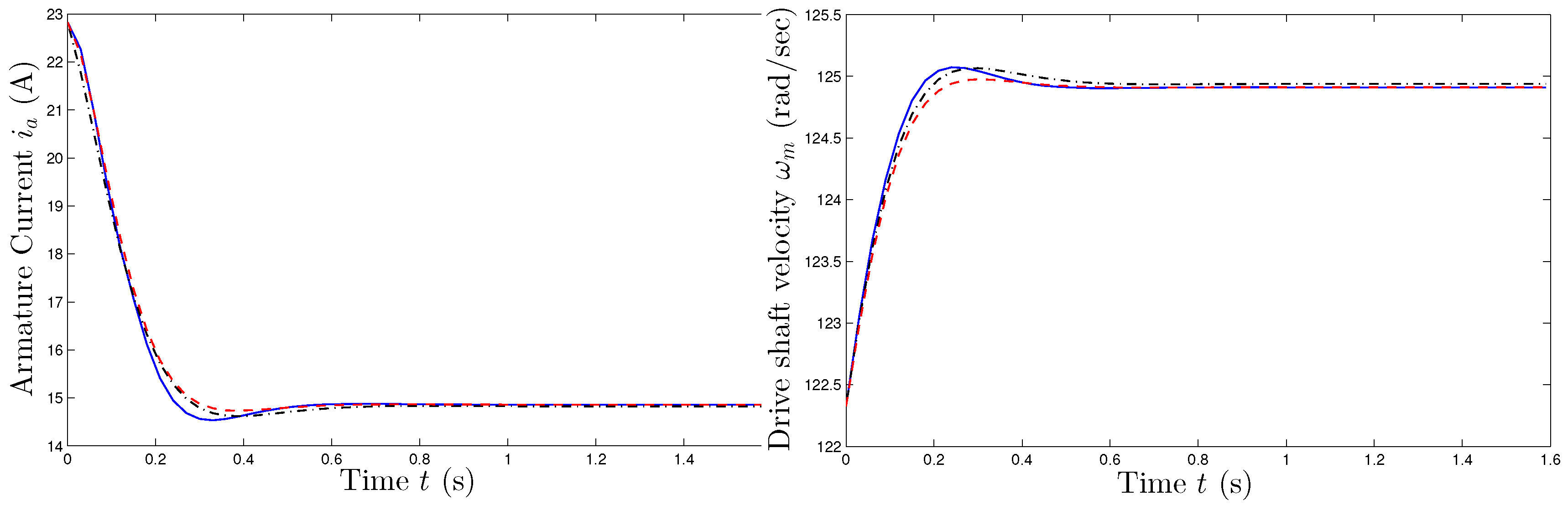
Figure 15.
Motor driven by a step armature voltage: Comparison of responses corresponding to the values of the parameters reported in
Table 25 and
Table 26. Blue-solid lines: Actual response. Red-crosshatched line: Response corresponding to the values of the parameters inferred upon doubling the search areas. Black dot-dashed lines: Response corresponding to the values of the parameters inferred upon quadrupling the search areas.
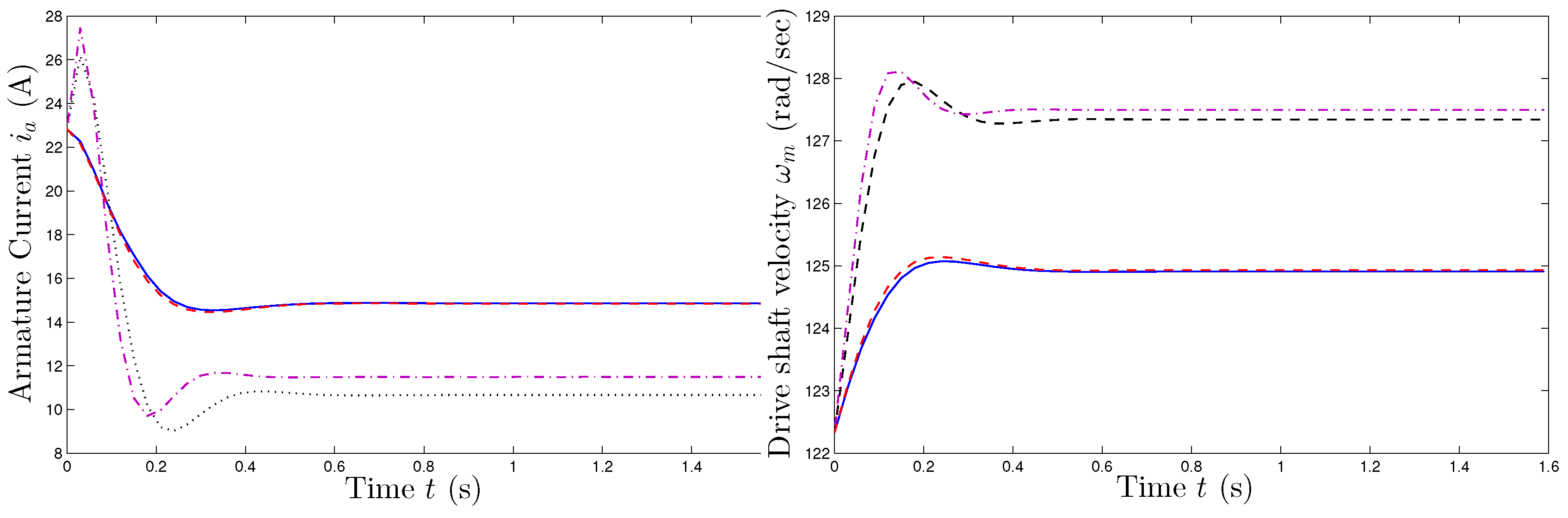
Figure 16.
Estimation of a DC motor parameters: A comparison of motor responses between models instantiated with parameters estimated by the R-COA, GA and SA algorithm. In the two panels, the solid (blue) lines denote the expected responses, the crosshatched (red) lines denote the results corresponding to the R-COA-based optimization, the dashed (black) lines denote the results pertaining to the GA-based optimization, while the dot-dashed (purple) lines correspond to the SA-based optimization.
Table 1.
Constraints and global minimum of the generalized Rosenbrock function (benchmark function “F1”) for the case of independent variables.
Table 1.
Constraints and global minimum of the generalized Rosenbrock function (benchmark function “F1”) for the case of independent variables.
| Constraints | Global Minimum |
|---|
| ; |
Table 2.
Constraints and global minimum of the Goldstein–Price function (benchmark function “F3”).
Table 2.
Constraints and global minimum of the Goldstein–Price function (benchmark function “F3”).
| Constraints | Global Minimum |
|---|
| ; , |
Table 3.
Constraints and global minimum of the Schaffer function (benchmark function “F4”).
Table 3.
Constraints and global minimum of the Schaffer function (benchmark function “F4”).
| Constraints | Global Minimum |
|---|
| ; |
Table 4.
Constraints and global minimum of the “step” function (benchmark function “F5”) for the case of independent variables.
Table 4.
Constraints and global minimum of the “step” function (benchmark function “F5”) for the case of independent variables.
| Constraints | Global Minimum |
|---|
| ; |
Table 5.
Constraints and global minimum of the Schwefel function (benchmark function “F6”) for the case of independent variables.
Table 5.
Constraints and global minimum of the Schwefel function (benchmark function “F6”) for the case of independent variables.
| Constraints | Global Minimum |
|---|
| ; |
Table 6.
Constraints and global minimum of the Rastring function (benchmark function “F7”) for the case of independent variables.
Table 6.
Constraints and global minimum of the Rastring function (benchmark function “F7”) for the case of independent variables.
| Constraints | Global Minimum |
|---|
| ; |
Table 7.
Results of the application of a rough search (only first carrier wave) on the benchmark functions F1 and F2.
Table 7.
Results of the application of a rough search (only first carrier wave) on the benchmark functions F1 and F2.
| F1 | F2 |
|---|
| Map | | Total Loops | Error | Map | | Total Loops | Error |
|---|
| Logistic | 400 | 553 | 7.90% | Logistic | 100 | 100 | 2.00% |
| Quadratic | 1000 | 3210 | 3.50% | Quadratic | 100 | 100 | 2.00% |
| Sine | 100 | 108 | 9.80% | Sine | 100 | 100 | 2.00% |
| Tent | 100 | 108 | 8.00% | Tent | 100 | 100 | 2.00% |
Table 8.
Results of the application of a rough search (only first carrier wave) on the benchmark functions F3 and F4.
Table 8.
Results of the application of a rough search (only first carrier wave) on the benchmark functions F3 and F4.
| F3 | F4 |
|---|
| Map | | Total Loops | Error | Map | | Total Loops | Error |
|---|
| Logistic | 100 | 133 | 1.75% | Logistic | 100 | 100 | 0.00% |
| Quadratic | 600 | 1431 | 0.20 % | Quadratic | 100 | 3526 | 0.00 % |
| Sine | 400 | 632 | 1.60% | Sine | 800 | 141 | 0.00% |
| Tent | 400 | 826 | 1.80% | Tent | 100 | 114 | 0.00% |
Table 9.
Results of the application of a rough search (only first carrier wave) on the benchmark functions F6 and F7.
Table 9.
Results of the application of a rough search (only first carrier wave) on the benchmark functions F6 and F7.
| F6 | F7 |
|---|
| Map | | Total Loops | Error | Map | | Total Loops | Error |
|---|
| Logistic | 600 | 1010 | 1.26% | Logistic | 100 | 100 | 2.00% |
| Quadratic | 100 | 177 | 2.60 % | Quadratic | 400 | 588 | 9.90 % |
| Sine | 600 | 1067 | 2.00% | Sine | 100 | 100 | 2.00% |
| Tent | 800 | 1516 | 4.00% | Tent | 100 | 116 | 1.80% |
Table 10.
Results of the application of a fine search (both first and second carrier waves) on the benchmark functions F1–F7.
Table 10.
Results of the application of a fine search (both first and second carrier waves) on the benchmark functions F1–F7.
| Benchmark Functions | Coordinates of GlobalMinimum | | Total Loops | | | P |
|---|
| F1 | | 200 | 1032 | | | |
| 2000 | 4500 | 0.9996 | 0.9976 | |
| F2 | | 1000 | 1568 | | | |
| 2000 | 7806 | 0.0006 | 0.0002 | |
| F3 | | 100 | 1228 | | | |
| 20,000 | 60,013 | | | |
| F4 | | 200 | 538 | 0.7312 | 1.3886 | |
| F5 | | 100 | 137 | | | - |
| F6 | | 100 | 1239 | 421.1416 | 420.9193 | |
| 15,000 | 34,855 | 420.9656 | 420.9927 | |
| F7 | | 500 | 1068 | | | |
| 2100 | 7606 | | 0.0001 | |
Table 11.
Results of the application of a refined search (first, second and third carrier waves) on the benchmark functions F1–F3, F6, F7 (Since the functions F4 and F5 did not need a better optimization, they were not tested with the new algorithm).
Table 11.
Results of the application of a refined search (first, second and third carrier waves) on the benchmark functions F1–F3, F6, F7 (Since the functions F4 and F5 did not need a better optimization, they were not tested with the new algorithm).
| Benchmark Functions | Coordinates of Global Minimum | | Total Loops | | | P |
|---|
| F1 | | 1000 | 2812 | 0.9999 | 1.0008 | |
| F2 | | 300 | 851 | 0.0000 | 0.0001 | |
| F3 | | 800 | 2705 | | | |
|
| F6 | | 600 | 1884 | 420.9641 | 420.9719 | |
| F7 | | 100 | 438 | 0.0002 | 0.0005 | |
Table 12.
Values of the test functions resulting from the application of a refined search (first, second and third carrier waves) on the benchmark functions F1–F3, F6, F7. (The functions F4 and F5 were not tested).
Table 12.
Values of the test functions resulting from the application of a refined search (first, second and third carrier waves) on the benchmark functions F1–F3, F6, F7. (The functions F4 and F5 were not tested).
| Test Functions | Global Minimum | |
|---|
| F1 | 0 | |
| F2 | 0 | |
| F3 | | |
| F6 | | |
| F7 | 0 | |
Table 13.
Results of a comparison between the refined COA and the SA (Simulated Annealing Algorithm) on the benchmark functions F1–F7.
Table 13.
Results of a comparison between the refined COA and the SA (Simulated Annealing Algorithm) on the benchmark functions F1–F7.
| Function | Refined COA | Simulated Annealing |
|---|
| Estimates | Total Loops | Average Estimates | Standard Deviation | Average Iterations | Convergence |
|---|
| F1 | | 2812 | | 0.1038 | 1407 | 10 |
| | 0.2240 |
| F2 | | 851 | | 0.0000 | 1011 | 10 |
| | 0.0000 |
| F3 | | 2705 | | 0.0000 | 1011 | 10 |
| | 0.0000 |
| F4 | | 538 | | 0.0010 | 1639 | 10 |
| F5 | | 137 | | 0.0000 | 1011 | 10 |
| F6 | | 1884 | | 218.5777 | 2437 | 0 |
| | 189.6553 |
| F7 | | 438 | | 0.3159 | 2167 | 8 |
| | 0.3152 |
Table 14.
Results of a comparison between the refined COA and the GA (Genetic Algorithm) on the benchmark functions F1–F7.
Table 14.
Results of a comparison between the refined COA and the GA (Genetic Algorithm) on the benchmark functions F1–F7.
| Function | Refined COA | Genetic Algorithm |
|---|
| Estimates | Total Loops | Average Estimates | Standard Deviation | Average Iterations | Convergence |
|---|
| F1 | | 2812 | | 0.0974 | 1392 | 10 |
| | 0.1745 |
| F2 | | 851 | | 0.0000 | 1011 | 10 |
| | 0.0000 |
| F3 | | 2705 | | 1.2464 | 1186 | 3 |
| | 0.7942 |
| F4 | | 538 | | 0.0000 | 1040 | 10 |
| F5 | | 137 | | 0.0000 | 1010 | 10 |
| F6 | | 1884 | | 123.3547 | 1324 | 0 |
| | 126.5412 |
| F7 | | 438 | | 0.3146 | 1040 | 8 |
| | 0.4195 |
Table 15.
Results of a comparison between the specific refined COA and the generic refined COA on the benchmark functions F1–F7.
Table 15.
Results of a comparison between the specific refined COA and the generic refined COA on the benchmark functions F1–F7.
| Functions | Specific Refined COA | Generic Refined COA |
|---|
| Estimates | Total Loops | | Total Loops |
|---|
| F1 | | 2812 | | 2055 |
| |
| F2 | | 851 | | 2055 |
| |
| F3 | | 2705 | | 5283 |
| |
| F4 | | 538 | | 2055 |
| F6 | | 1884 | | 3662 |
| |
| F7 | | 438 | | 2105 |
| |
Table 16.
Application to DC motor model parameters estimation: Actual values of motor’s physical electro-mechanical parameters.
Table 16.
Application to DC motor model parameters estimation: Actual values of motor’s physical electro-mechanical parameters.
| Parameter | Parameter Symbol | Parameter Value |
|---|
| Armature Resistance | | 0.6 |
| Armature Inductance | | 0.03 H |
| Viscous Friction | | 0.1 N·m·s/rad |
| Rotor Inertia | | 0.6 kg·m/rad |
| Torque Coefficient | | 1.85 V·s/rad |
| Torque Load | | 15 N·m |
Table 17.
Application to DC motor model parameters estimation: Search range for each parameter based on physical constrains.
Table 17.
Application to DC motor model parameters estimation: Search range for each parameter based on physical constrains.
| Parameter | Parameter Symbol | Parameter Search Range |
|---|
| Armature Resistance | | 0.1–0.8 () |
| Armature Inductance | | 0.01–0.05 (H) |
| Viscous Friction | | 0.05–0.5 (N·m·s/rad) |
| Rotor Inertia | | 0.1–0.8 (kg·m/rad) |
| Torque Coefficient | | 1–2 (V·s/rad) |
| Torque Load | | 10–20 (N·m) |
Table 18.
Motor driven by a step armature voltage: Test on estimating the electrical model parameters only.
Table 18.
Motor driven by a step armature voltage: Test on estimating the electrical model parameters only.
| Carrier Wave | Total Loops | | Error | | Error | Total Error |
|---|
| First | 202 | 0.6156 | 0.0156 | 0.0320 | 0.0020 | 1.1003 |
| Second | 953 | 0.6003 | 0.0003 | 0.0301 | 0.0001 | 0.0601 |
Table 19.
Motor driven by a step armature voltage: Test on estimating the mechanical model parameters only.
Table 19.
Motor driven by a step armature voltage: Test on estimating the mechanical model parameters only.
| Carrier Wave | Total Loops | | Error | J | Error | Total Error |
|---|
| First | 272 | 0.0991 | 0.0009 | 0.6085 | 0.0085 | 1.0095 |
| Second | 432 | 0.0991 | 0.0009 | 0.6008 | 0.0008 | 0.0704 |
Table 20.
Motor driven by a step armature voltage: Weights analysis for the joint electrical and mechanical model parameters estimation.
Table 20.
Motor driven by a step armature voltage: Weights analysis for the joint electrical and mechanical model parameters estimation.
| | Total Loops | | | | J | K | Total Error |
|---|
| Actual Value | | 0.6 | 0.03 | 0.1 | 0.6 | 1.85 | |
|---|
| 521 | 0.5904 | 0.0295 | 0.0982 | 0.6388 | 1.8516 | 9.9568 |
| 5229 | 0.5942 | 0.0312 | 0.1001 | 0.6503 | 1.8505 | 7.3798 |
| 521 | 0.6029 | 0.0295 | 0.1005 | 0.6521 | 1.8504 | 7.9601 |
| 5229 | 0.5942 | 0.0312 | 0.1001 | 0.6503 | 1.8505 | 7.3798 |
| 582 | 0.5904 | 0.0295 | 0.0982 | 0.6399 | 1.8516 | 12.6972 |
| 7143 | 0.5926 | 0.0321 | 0.1001 | 0.6503 | 1.8505 | 8.9209 |
Table 21.
Motor driven by a step armature voltage: Joint electrical and mechanical model parameters estimation in the presence of a disturbance on the drive shaft velocity measurements.
Table 21.
Motor driven by a step armature voltage: Joint electrical and mechanical model parameters estimation in the presence of a disturbance on the drive shaft velocity measurements.
| | Total Loops | | | | J | K | Total Error |
|---|
| Actual value | | 0.6 | 0.03 | 0.1 | 0.6 | 1.85 | |
|---|
| 411 | 0.8000 | 0.0344 | 0.0703 | 0.2424 | 1.8328 | 139.2181 |
| 411 | 0.8000 | 0.0344 | 0.0703 | 0.2424 | 1.8328 | 139.2181 |
| 846 | 0.7993 | 0.0357 | 0.0888 | 0.5366 | 1.8010 | 114.2229 |
Table 22.
Motor driven by a step armature voltage: Full motor modeling results.
Table 22.
Motor driven by a step armature voltage: Full motor modeling results.
| | Loops | | | | J | K | | Error | Parameter Error |
|---|
| Actual value | | 0.6 | 0.03 | 0.1 | 0.6 | 1.85 | 15 | | |
|---|
| First carrier | 1608 | 0.7693 | 0.0235 | 0.2053 | 0.7687 | 1.8285 | 13.5296 | 28.9436 | 5.1975 |
| Second carrier | 1766 | 0.6346 | 0.0339 | 0.0954 | 0.5253 | 1.8432 | 15.9757 | 18.0243 | 1.6334 |
| Third carrier | 1928 | 0.5594 | 0.0280 | 0.1004 | 0.5705 | 1.8551 | 15.5225 | 4.7574 | 0.9623 |
| 4624 | 0.6274 | 0.3370 | 0.0992 | 0.5645 | 1.8465 | 15.6379 | 4.3600 | 1.0743 |
Table 23.
Motor driven by a step armature voltage: Actual steady-state values versus predicted values.
Table 23.
Motor driven by a step armature voltage: Actual steady-state values versus predicted values.
| Armature Current | Drive Shaft Velocity |
|---|
| 148,600 | | 1,249,102 |
| 148,379 | | 1,249,340 |
Table 24.
Motor driven by a step armature voltage: Ranges for the parameters search areas doubled and quadrupled with respect to the values indicated in
Table 17.
Table 24.
Motor driven by a step armature voltage: Ranges for the parameters search areas doubled and quadrupled with respect to the values indicated in
Table 17.
| Constrains Expansion | | | | J | K | |
|---|
| Doubling | 0.1–1.5 | 0.01–0.09 | 0.05–0.95 | 0.1–1.5 | 1–3 | 10–20 |
| Quadrupling | 0.1–2.9 | 0.01–0.17 | 0.05–1.85 | 0.1–2.9 | 1–5 | 10–50 |
Table 25.
Motor driven by a step armature voltage: Results of parameters estimation by R-COA on doubled search areas.
Table 25.
Motor driven by a step armature voltage: Results of parameters estimation by R-COA on doubled search areas.
| | Total Loops | | | | J | K | | Total Error | Parameter Error |
|---|
| Actual value | | 0.6 | 0.03 | 0.1 | 0.6 | 1.85 | 15 | | |
|---|
| First carrier | 271 | 0.7077 | 0.0291 | 0.2256 | 0.3888 | 1.9174 | 11.6350 | 337.2882 | 10.7149 |
| Second carrier | 429 | 0.6041 | 0.0335 | 0.1051 | 0.6420 | 1.8668 | 15.9271 | 104.4469 | 4.9715 |
| Third carrier | 1531 | 0.5830 | 0.0306 | 0.1008 | 0.6645 | 1.8553 | 15.0930 | 12.6643 | 0.8976 |
| 9037 | 0.6260 | 0.0297 | 0.0996 | 0.6589 | 1.8469 | 16.1967 | 4.7691 | 1.0058 |
Table 26.
Motor driven by a step armature voltage: Results of parameters estimation by R-COA on quadrupled search areas.
Table 26.
Motor driven by a step armature voltage: Results of parameters estimation by R-COA on quadrupled search areas.
| | Total Loops | | | | J | K | | Total Error | Parameter Error |
|---|
| Actual value | | 0.6 | 0.03 | 0.1 | 0.6 | 1.85 | 15 | | |
|---|
| First carrier | 123 | 1.3366 | 0.1448 | 0.2094 | 0.8115 | 1.8609 | 16.45778 | 375.5978 | 22.2117 |
| Second carrier | 233 | 1.0405 | 0.0473 | 0.0959 | 0.2330 | 1.7996 | 16.1008 | 72.0653 | 7.0065 |
| Third carrier | 1349 | 0.5338 | 0.0312 | 0.0998 | 0.6371 | 1.8534 | 16.1937 | 24.6221 | 1.2778 |
| 2582 | 0.7516 | 0.0429 | 0.0973 | 0.5987 | 1.8534 | 15.4716 | 6.7405 | 1.8114 |
Table 27.
Estimation of a DC motor parameters: Comparison of the R-COA with the SA algorithm and the GA.
Table 27.
Estimation of a DC motor parameters: Comparison of the R-COA with the SA algorithm and the GA.
| | | Results |
|---|
| | Algorithm | R-COA | GA | SA |
|---|
| | Total Loops | 4624 | 1578 | 9767 |
| 0.6 | 0.6274 | 0.4048 | 0.3873 |
| 0.03 | 0.0337 | 0.0183 | 0.0139 |
| 0.1 | 0.0992 | 0.0511 | 0.0500 |
| 0.6 | 0.5645 | 0.5147 | 0.4123 |
| 1.85 | 1.8465 | 1.8508 | 1.8475 |
| 15 | 15.6379 | 13.2203 | 14.8479 |
| | Total Error | 4.3600 | 204.1683 | 242.6949 |
| | Parameter Error | 1.0743 | 4.6403 | 6.1314 |


