Robust-BD Estimation and Inference for General Partially Linear Models

Abstract

The classical quadratic loss for the partially linear model (PLM) and the likelihood function for the generalized PLM are not resistant to outliers. This inspires us to propose a class of “robust-Bregman divergence (BD)” estimators of both the parametric and nonparametric components in the general partially linear model (GPLM), which allows the distribution of the response variable to be partially specified, without being fully known. Using the local-polynomial function estimation method, we propose a computationally-efficient procedure for obtaining “robust-BD” estimators and establish the consistency and asymptotic normality of the “robust-BD” estimator of the parametric component ${\mathit{\beta }}_{\mathrm{o}}$. For inference procedures of ${\mathit{\beta }}_{\mathrm{o}}$ in the GPLM, we show that the Wald-type test statistic $W_n$ constructed from the “robust-BD” estimators is asymptotically distribution free under the null, whereas the likelihood ratio-type test statistic ${\Lambda }_n$ is not. This provides an insight into the distinction from the asymptotic equivalence (Fan and Huang 2005) between $W_n$ and ${\Lambda }_n$ in the PLM constructed from profile least-squares estimators using the non-robust quadratic loss. Numerical examples illustrate the computational effectiveness of the proposed “robust-BD” estimators and robust Wald-type test in the appearance of outlying observations.

1. Introduction

Semiparametric models, such as the partially linear model (PLM) and generalized PLM, play an important role in statistics, biostatistics, economics and engineering studies [1,2,3,4,5]. For the response variable Y and covariates $(\mathit{X},T)$, where $\mathit{X}={(X_1,\dots ,X_d)}^T\in {\mathbb{R}}^d$ and $T\in \mathcal{T}\subseteq {\mathbb{R}}^D$, the PLM, which is widely used for continuous responses Y, describes the model structure according to:

$$Y={\mathit{X}}^T{\mathit{\beta }}_{\mathrm{o}}+{\eta }^{\mathrm{o}}\left(T\right)+ϵ,\mathrm{E}(ϵ\mid \mathit{X},T)=0,$$

(1)

where ${\mathit{\beta }}_{\mathrm{o}}={({\beta }_{1;\mathrm{o}},\dots ,{\beta }_{d;\mathrm{o}})}^T$ is a vector of unknown parameters and ${\eta }^{\mathrm{o}}(·)$ is an unknown smooth function; the generalized PLM, which is more suited to discrete responses Y and extends the generalized linear model [6], assumes:

$$\begin{array}{c}m(\mathit{x},t)=\mathrm{E}(Y\mid \mathit{X}=\mathit{x},T=t)=F^{-1}({\mathit{x}}^T{\mathit{\beta }}_{\mathrm{o}}+{\eta }^{\mathrm{o}}\left(t\right)),\hfill \end{array}$$

(2)

$$\begin{array}{c}Y\mid (\mathit{X},T)\sim \mathrm{exponential}\mathrm{family}\mathrm{of}\mathrm{distributions},\hfill \end{array}$$

(3)

where F is a known link function. Typically, the parametric component ${\mathit{\beta }}_{\mathrm{o}}$ is of primary interest, while the nonparametric component ${\eta }^{\mathrm{o}}(·)$ serves as a nuisance function. For illustration clarity, this paper focuses on $D=1$. An important application of PLM to brain fMRI data was given in [7] for detecting activated brain voxels in response to external stimuli. There, ${\mathit{\beta }}_{\mathrm{o}}$ corresponds to the part of hemodynamic response values, which is the object of primary interest to neuroscientists; ${\eta }^{\mathrm{o}}(·)$ is the slowly drifting baseline of time. Determining whether a voxel is activated or not can be formulated as testing for the linear form of hypotheses,

$$H_0:\mathrm{A}{\mathit{\beta }}_{\mathrm{o}}={\mathit{g}}_0\mathrm{versus}{H}_1:\mathrm{A}{\mathit{\beta }}_{\mathrm{o}}\ne {\mathit{g}}_0,$$

(4)

where $\mathrm{A}$ is a given $\mathsf{k}\times d$ full row rank matrix and ${\mathit{g}}_0$ is a known $\mathsf{k}\times 1$ vector.

Estimation of the parametric and nonparametric components of PLM and generalized PLM has received much attention in the literature. On the other hand, the existing work has some limitations: (i) The generalized PLM assumes that $Y\mid (\mathit{X},T)$ follows the distribution in (3), so that the likelihood function is fully available. From the practical viewpoint, results from the generalized PLM are not applicable to situations where the distribution of $Y\mid (\mathit{X},T)$ either departs from (3) or is incompletely known. (ii) Some commonly-used error measures, such as the quadratic loss in PLM for Gaussian-type responses (see for example [7,8]) and the (negative) likelihood function used in the generalized PLM, are not resistant to outliers. The work in [9] studied robust inference based on the kernel regression method for the generalized PLM with a canonical link, based on either the (negative) likelihood or (negative) quasi-likelihood as the error measure, and illustrated numerical examples with the dimension $d=1$. However, the quasi-likelihood is not suitable for the exponential loss function (defined in Section 2.1), commonly used in machine learning and data mining. (iii) The work in [8] developed the inference of (4) for PLM, via the classical quadratic loss as the error measure, and demonstrated that the asymptotic distributions of the likelihood ratio-type statistic and Wald statistic under the null of (4) are both ${\chi }_{\mathsf{k}}^2$. It remains unknown whether this conclusion holds when the tests are constructed based on robust estimators.

Without completely specifying the distribution of $Y\mid (\mathit{X},T)$, we assume:

$$\mathrm{var}(Y\mid \mathit{X}=\mathit{x},T=t)=V\left(m\right(\mathit{x},t\left)\right),$$

(5)

with a known functional form of $V(·)$. We refer to a model specified by (2) and (5) as the “general partially linear model” (GPLM). This paper aims to develop robust estimation of GPLM and robust inference of ${\mathit{\beta }}_{\mathrm{o}}$, allowing the distribution of $Y\mid (\mathit{X},T)$ to be partially specified. To introduce robust estimation, we adopt a broader class of robust error measures, called “robust-Bregman divergence (BD)” developed in [10], for a GLM, in which BD includes the quadratic loss, the (negative) quasi-likelihood, the exponential loss and many other commonly-used error measures as special cases. We propose the “robust-BD estimators” for both the parametric and nonparametric components of the GPLM. Distinct from the explicit-form estimators for PLM using the classical quadratic loss (see [8]), the “robust-BD estimators” for GPLM do not have closed-form expressions, which makes the theoretical derivation challenging. Moreover, the robust-BD estimators, as numerical solutions to non-linear optimization problems, pose key implementation challenges. Our major contributions are given below.

• The robust fitting of the nonparametric component ${\eta }^{\mathrm{o}}(·)$ is formulated using the local-polynomial regression technique [11]. See Section 2.3.
• We develop a coordinate descent algorithm for the robust-BD estimator of ${\mathit{\beta }}_{\mathrm{o}}$, which is computationally efficient particularly when the dimension d is large. See Section 3.
• Theorems 1 and 2 demonstrate that under the GPLM, the consistency and asymptotic normality of the proposed robust-BD estimator for ${\mathit{\beta }}_{\mathrm{o}}$ are achieved. See Section 4.
• For robust inference of ${\mathit{\beta }}_{\mathrm{o}}$, we propose a robust version of the Wald-type test statistic $W_n$, based on the robust-BD estimators, and justify its validity in Theorems 3–5. It is shown to be asymptotically ${\chi }^2$ (central) under the null, thus distribution free, and ${\chi }^2$ (noncentral) under the contiguous alternatives. Hence, this result, when applied to the exponential loss, as well as other loss functions in the wider class of BD, is practically feasible. See Section 5.1.
• For robust inference of ${\mathit{\beta }}_{\mathrm{o}}$, we re-examine the likelihood ratio-type test statistic ${\Lambda }_n$, constructed by replacing the negative log-likelihood with the robust-BD. Our Theorem 6 reveals that the asymptotic null distribution of ${\Lambda }_n$ is generally not ${\chi }^2$, but a linear combination of independent ${\chi }^2$ variables, with weights relying on unknown quantities. Even in the particular case of using the classical-BD, the limit distribution is not invariant with re-scaling the generating function of the BD. Moreover, the limit null distribution of ${\Lambda }_n$ (in either the non-robust or robust version) using the exponential loss, which does not belong to the (negative) quasi-likelihood, but falls in BD, is always a weighted ${\chi }^2$, thus limiting its use in practical applications. See Section 5.2.

Simulation studies in Section 6 demonstrate that the proposed class of robust-BD estimators and robust Wald-type test either compare well with or perform better than the classical non-robust counterparts: the former is less sensitive to outliers than the latter, and both perform comparably well for non-contaminated cases. Section 7 illustrates some real data applications. Section 8 ends the paper with brief discussions. Details of technical derivations are relegated to Appendix A.

2. Robust-BD and Robust-BD Estimators

This section starts with a brief review of BD in Section 2.1 and “robust-BD” in Section 2.2, followed by the proposed “robust-BD” estimators of ${\eta }^{\mathrm{o}}(·)$ and ${\mathit{\beta }}_{\mathrm{o}}$ in Section 2.3 and Section 2.4.

2.1. Classical-BD

To broaden the scope of robust estimation and inference, we consider a class of error measures motivated from the Bregman divergence (BD). For a given concave q-function, [12] defined a bivariate function,

$$Q_q(\nu ,\mu )=-q\left(\nu \right)+q\left(\mu \right)+(\nu -\mu )q^{\prime }\left(\mu \right).$$

(6)

We call $Q_q$ the BD and call q the generating q-function of the BD. For example, a function $q\left(\mu \right)=a\mu -{\mu }^2$ for some constant a yields the quadratic loss $Q_q(Y,\mu )={(Y-\mu )}^2$. For a binary response variable Y, $q\left(\mu \right)=\min \{\mu ,(1-\mu \left)\right\}$ gives the misclassification loss $Q_q(Y,\mu )=\mathrm{I}\{Y\ne \mathrm{I}(\mu >1/2)\}$, where $\mathrm{I}(·)$ is an indicator function; $q\left(\mu \right)=-2\left\{\mu \log \right(\mu )+(1-\mu \left)\log \right(1-\mu \left)\right\}$ gives the Bernoulli deviance loss log-likelihood $Q_q(Y,\mu )=-2\{Y\log \left(\mu \right)+(1-Y)\log (1-\mu )\}$; $q\left(\mu \right)=2\min \{\mu ,(1-\mu \left)\right\}$ results in the hinge loss $Q_q(Y,\mu )=\max \{1-(2Y-1)\mathrm{sign}(\mu -0.5),0\}$ of the support vector machine; $q\left(\mu \right)=2{\left\{\mu (1-\mu )\right\}}^{1/2}$ yields the exponential loss $Q_q(Y,\mu )=\exp [-(Y-0.5)\log \{\mu /(1-\mu )\}]$ used in AdaBoost [13]. Moreover, [14] showed that if:

$$q\left(\mu \right)={\int }_a^{\mu }\frac{s-\mu }{V\left(s\right)}ds,$$

(7)

with a finite constant a such that the integral is well defined, then $Q_q(y,\mu )$ matches the “classical (negative) quasi-likelihood” function.

2.2. Robust-BD ${\rho }_q(y,\mu )$

Let $r(y,\mu )=(y-\mu )/\sqrt{V\left(\mu \right)}$ denote the Pearson residual, which reduces to the standardized residual for linear models. In contrast to the “classical-BD”, denoted by $Q_q$ in (6), the “robust-BD” developed in [10] for a GLM [6], is formed by:

$${\rho }_q(y,\mu )={\int }_y^{\mu }\psi \left(r(y,s)\right)\left\{q^{″}\left(s\right)\sqrt{V\left(s\right)}\right\}ds-G\left(\mu \right),$$

(8)

where $\psi \left(r\right)$ is chosen to be a bounded, odd function, such as the Huber $\psi$-function [15], $\psi \left(r\right)=r\min (1,c/|r\left|\right)$, and the bias-correction term, $G\left(\mu \right)$, entails the Fisher consistency of the parameter estimator and satisfies:

$$G^{\prime }\left(\mu \right)=G_1^{\prime }\left(\mu \right)\left\{q^{″}\left(\mu \right)\sqrt{V\left(\mu \right)}\right\},$$

with

$$G_1^{\prime }\left(m(\mathit{x},t)\right)=\mathrm{E}\{\psi \left(r(Y,m(\mathit{x},t))\right)\mid \mathit{X}=\mathit{x},T=t\}.$$

(9)

We make the following discussions regarding features of the “robust-BD”. To facilitate the discussion, we first introduce some necessary notation. Assume that the quantities:

$${\mathrm{p}}_j(y;\theta )=\frac{{\partial }^j}{\partial {\theta }^j}{\rho }_q(y,F^{-1}\left(\theta \right)),j=0,1,\dots ,$$

(10)

exist finitely up to any order required. Then, we have the following expressions,

$$\begin{array}{ccc}\hfill {\mathrm{p}}_1(y;\theta )& =& \{\psi \left(r(y,\mu )\right)-G_1^{\prime }\left(\mu \right)\}\left\{q^{″}\left(\mu \right)\sqrt{V\left(\mu \right)}\right\}/F^{\prime }\left(\mu \right),\hfill \\ \hfill {\mathrm{p}}_2(y;\theta )& =& A_0(y,\mu )+\{\psi \left(r(y,\mu )\right)-G_1^{\prime }\left(\mu \right)\}{A}_1\left(\mu \right),\hfill \\ \hfill {\mathrm{p}}_3(y;\theta )& =& A_2(y,\mu )+\{\psi \left(r(y,\mu )\right)-G_1^{\prime }\left(\mu \right)\}{A}_1^{\prime }\left(\mu \right)/F^{\prime }\left(\mu \right),\hfill \end{array}$$

(11)

where $\mu =F^{-1}\left(\theta \right)$,

$$A_0(y,\mu )=-\left[{\psi }^{\prime }\left(r(y,\mu )\right)\left\{1+\frac{y-\mu }{\sqrt{V\left(\mu \right)}}\times \frac{V^{\prime }\left(\mu \right)}{2\sqrt{V\left(\mu \right)}}\right\}+G_1^{″}\left(\mu \right)\sqrt{V\left(\mu \right)}\right]\frac{q^{″}\left(\mu \right)}{{\left\{F^{\prime }\left(\mu \right)\right\}}^2},$$

$A_1\left(\mu \right)=[\{q^{\left(3\right)}\left(\mu \right)\sqrt{V\left(\mu \right)}+2^{-1}{q}^{″}\left(\mu \right)V^{\prime }\left(\mu \right)/\sqrt{V\left(\mu \right)}\}{F}^{\prime }\left(\mu \right)-q^{″}\left(\mu \right)\sqrt{V\left(\mu \right)}{F}^{″}\left(\mu \right)]/{\left\{F^{\prime }\left(\mu \right)\right\}}^3$ and $A_2(y,\mu )=[\partial A_0(y,\mu )/\partial \mu +\partial \{\psi \left(r(y,\mu )\right)-G_1^{\prime }\left(\mu \right)\}/\partial \mu A_1\left(\mu \right)]/F^{\prime }\left(\mu \right)$. Particularly, ${\mathrm{p}}_1(y;\theta )$ contains $\psi \left(r\right)$; ${\mathrm{p}}_2(y;\theta )$ contains $\psi \left(r\right)$, ${\psi }^{\prime }\left(r\right)$ and ${\psi }^{\prime }\left(r\right)r$; ${\mathrm{p}}_3(y;\theta )$ contains $\psi \left(r\right)$, ${\psi }^{\prime }\left(r\right)$, ${\psi }^{\prime }\left(r\right)r$, ${\psi }^{″}\left(r\right)$, ${\psi }^{″}\left(r\right)r$, and ${\psi }^{″}\left(r\right)r^2$, where $r=r(y,\mu )=(y-\mu )/\sqrt{V\left(\mu \right)}$ denotes the Pearson residual. Accordingly, $\{{\mathrm{p}}_j(y;\theta ):j=1,2,3\}$ depend on y through $\psi \left(r\right)$ and its derivatives coupled with r. Then, we observe from (9) and (11) that:

$$\mathrm{E}\{{\mathrm{p}}_1(Y;{\mathit{X}}^T{\mathit{\beta }}_{\mathrm{o}}+{\eta }^{\mathrm{o}}\left(T\right))\mid \mathit{X},T\}=0.$$

(12)

In the particular choice of $\psi \left(r\right)=r$, it is clearly noticed from (9) that $G_1^{\prime }(·)=0$, and thus, $G^{\prime }(·)=0$. In such a case, the proposed “robust-BD” ${\rho }_q(y,\mu )$ reduces to the “classical-BD” $Q_q(y,\mu )$.

2.3. Local-Polynomial Robust-BD Estimator of ${\eta }^{\mathrm{o}}(·)$

Let ${\left\{(Y_i,{\mathit{X}}_i,T_i)\right\}}_{i=1}^n$ be $\mathrm{i}.\mathrm{i}.\mathrm{d}.$ observations of $(Y,\mathit{X},T)$ captured by the GPLM in (2) and (5), where the dimension $d\ge 1$ is a finite integer. From (2), it is directly observed that if the true value of ${\mathit{\beta }}_{\mathrm{o}}$ is known, then estimating ${\eta }^{\mathrm{o}}(·)$ becomes estimating a nonparametric function; conversely, if the actual form of ${\eta }^{\mathrm{o}}(·)$ is available, then estimating ${\mathit{\beta }}_{\mathrm{o}}$ amounts to estimating a vector parameter.

To motivate the estimation of ${\eta }^{\mathrm{o}}(·)$ at a fitting point t, a proper way to characterize ${\eta }^{\mathrm{o}}\left(t\right)$ is desired. For any given value of $\mathit{\beta }$, define:

$$S(a;t,\mathit{\beta })=\mathrm{E}\{{\rho }_q(Y,F^{-1}({\mathit{X}}^T\mathit{\beta }+a))w_1\left(\mathit{X}\right)\mid T=t\},$$

(13)

where a is a scalar, ${\rho }_q(y,\mu )$ is the “robust-BD” defined in (8), which aims to guard against outlying observations in the response space of Y, and $w_1(·)\ge 0$ is a given bounded weight function that downweights high leverage points in the covariate space of $\mathit{X}$. See Section 6 and Section 7 for an example of $w_1\left(\mathit{x}\right)$. Set:

$${\eta }_{\mathit{\beta }}\left(t\right)=\arg \underset{a\in {\mathbb{R}}^1}{\min }S(a;t,\mathit{\beta }).$$

(14)

Theoretically, ${\eta }^{\mathrm{o}}\left(t\right)={\eta }_{{\mathit{\beta }}_{\mathrm{o}}}\left(t\right)$ will be assumed (in Condition A3) for obtaining asymptotically unbiased estimators of ${\eta }^{\mathrm{o}}(·)$. Such property indeed holds, for example, when a classical quadratic loss combined with an identity link is used in (14). Thus, we call ${\eta }_{\mathit{\eta }}(·)$ the “surrogate function” for ${\eta }^{\mathrm{o}}(·)$.

The characterization of the surrogate function ${\mathit{\eta }}_{\beta }\left(t\right)$ in (14) enables us to develop its robust-BD estimator ${\widehat{\eta }}_{\mathit{\beta }}\left(t\right)$ based on nonparametric function estimation. Assume that ${\eta }^{\mathrm{o}}(·)$ is $(p+1)$-times continuously differentiable at the fitting point t. Denote by ${\mathbf{a}}_{\mathrm{o}}\left(t\right)={({\eta }^{\mathrm{o}}\left(t\right),{\left({\eta }^{\mathrm{o}}\right)}^{\left(1\right)}\left(t\right),\dots ,{\left({\eta }^{\mathrm{o}}\right)}^{\left(p\right)}\left(t\right)/p!)}^T\in {\mathbb{R}}^{p+1}$ the vector consisting of ${\eta }^{\mathrm{o}}\left(t\right)$ along with its (re-scaled) derivatives. For observed covariates $T_i$ close to the point t, the Taylor expansion implies that:

$$\begin{array}{ccc}\hfill {\eta }^{\mathrm{o}}\left(T_i\right)& \approx & {\eta }^{\mathrm{o}}\left(t\right)+(T_i-t){\left({\eta }^{\mathrm{o}}\right)}^{\left(1\right)}\left(t\right)+\cdots +{(T_i-t)}^p{\left({\eta }^{\mathrm{o}}\right)}^{\left(p\right)}\left(t\right)/p!\hfill \\ & =& {\mathbf{t}}_i{\left(t\right)}^T{\mathbf{a}}_{\mathrm{o}}\left(t\right),\hfill \end{array}$$

(15)

where ${\mathbf{t}}_i\left(t\right)={(1,(T_i-t),\dots ,{(T_i-t)}^p)}^T$. For any given value of $\mathit{\beta }$, let $\widehat{\mathit{a}}(t;\mathit{\beta })={({\widehat{a}}_0(t;\mathit{\beta }),{\widehat{a}}_1(t;\mathit{\beta }),\dots ,{\widehat{a}}_p(t;\mathit{\beta }))}^T$ be the minimizer of the criterion function,

$$S_n(\mathit{a};t,\mathit{\beta })=\frac{1}{n}{\displaystyle \sum _{i=1}^n}{\rho }_q(Y_i,F^{-1}({\mathit{X}}_i^T\mathit{\beta }+{\mathbf{t}}_i{\left(t\right)}^T\mathit{a}))w_1\left({\mathit{X}}_i\right)K_h(T_i-t),$$

(16)

with respect to $\mathit{a}\in {\mathbb{R}}^{p+1}$, where $K_h(·)=K(·/h)/h$ is re-scaled from a kernel function K and $h>0$ is termed a bandwidth parameter. The first entry of $\widehat{\mathit{a}}(t;\mathit{\beta })$ supplies the local-polynomial robust-BD estimator ${\widehat{\eta }}_{\mathit{\beta }}\left(t\right)$ of ${\eta }_{\mathit{\beta }}\left(t\right)$, i.e.,

$${\widehat{\eta }}_{\mathit{\beta }}\left(t\right)={\mathit{e}}_{1,p+1}^T\left\{\arg \underset{\mathit{a}\in {\mathbb{R}}^{p+1}}{\min }{S}_n(\mathit{a};t,\mathit{\beta })\right\},$$

(17)

where ${\mathit{e}}_{j,p+1}$ denotes the j-th column of a $(p+1)\times (p+1)$ identity matrix.

It is noted that the reliance of ${\widehat{\eta }}_{\mathit{\beta }}\left(t\right)$ on $\mathit{\beta }$ does not guarantee its consistency to ${\eta }^{\mathrm{o}}\left(t\right)$. Nonetheless, it is anticipated from the uniform consistency of ${\widehat{\eta }}_{\widehat{\mathit{\beta }}}$ in Lemma 1 that ${\widehat{\eta }}_{\widehat{\mathit{\beta }}}\left(t\right)$ will offer a valid estimator of ${\eta }^{\mathrm{o}}\left(t\right)$, provided that $\widehat{\mathit{\beta }}$ consistently estimates ${\mathit{\beta }}_{\mathrm{o}}$. Section 2.4 will discuss our proposed robust-BD estimator $\widehat{\mathit{\beta }}$. Furthermore, Lemma 1 will assume (in Condition A1) that ${\eta }_{\mathit{\beta }}\left(t\right)$ is the unique minimizer of $S(a;t,\mathit{\beta })$ with respect to a.

Remark 1.

The case of using the “kernel estimation”, or locally-constant estimation, corresponds to the choice of degree $p=0$ in (15). In that case, the criterion function in (16) and the estimator in (17) reduce to:

$$\begin{array}{ccc}\hfill S_n(a;t,\mathit{\beta })& =& \frac{1}{n}{\displaystyle \sum _{i=1}^n}{\rho }_q(Y_i,F^{-1}({\mathit{X}}_i^T\mathit{\beta }+a))w_1\left({\mathit{X}}_i\right)K_h(T_i-t),\hfill \end{array}$$

(18)

$$\begin{array}{ccc}\hfill {\widehat{\eta }}_{\mathit{\beta }}\left(t\right)& =& \arg \underset{a\in {\mathbb{R}}^1}{\min }{S}_n(a;t,\mathit{\beta }),\hfill \end{array}$$

(19)

respectively.

2.4. Robust-BD Estimator of ${\beta }_{\mathrm{o}}$

For any given value of $\mathit{\beta }$, define:

$$J(\mathit{\beta },{\eta }_{\mathit{\beta }})=\mathrm{E}\left\{{\rho }_q(Y,F^{-1}({\mathit{X}}^T\mathit{\beta }+{\eta }_{\mathit{\beta }}\left(T\right)))w_2\left(\mathit{X}\right)\right\},$$

(20)

where ${\eta }_{\mathit{\beta }}(·)$ is as defined in (14) and $w_2(·)$ plays the same role as $w_1(·)$ in (13). Theoretically, it is anticipated that:

$${\mathit{\beta }}_{\mathrm{o}}=\arg \underset{\mathit{\beta }\in {\mathbb{R}}^d}{\min }J(\mathit{\beta },{\eta }_{\mathit{\beta }}),$$

(21)

which holds for example in the case where a classical quadratic loss combined with an identity link is used. To estimate ${\mathit{\beta }}_{\mathrm{o}}$, it is natural to replace (20) by its sample-based criterion,

$$J_n(\mathit{\beta },{\widehat{\eta }}_{\mathit{\beta }})=\frac{1}{n}{\displaystyle \sum _{i=1}^n}{\rho }_q(Y_i,F^{-1}({\mathit{X}}_i^T\mathit{\beta }+{\widehat{\eta }}_{\mathit{\beta }}\left(T_i\right)))w_2\left({\mathit{X}}_i\right),$$

(22)

where ${\widehat{\eta }}_{\mathit{\beta }}(·)$ is as defined in (17). Hence, a parametric estimator of ${\mathit{\beta }}_{\mathrm{o}}$ is provided by:

$$\widehat{\mathit{\beta }}=\arg \underset{\mathit{\beta }\in {\mathbb{R}}^d}{\min }{J}_n(\mathit{\beta },{\widehat{\eta }}_{\mathit{\beta }}).$$

(23)

Finally, the estimator of ${\eta }^{\mathrm{o}}(·)$ is given by:

$$\widehat{\eta }(·)={\widehat{\eta }}_{\widehat{\mathit{\beta }}}(·).$$

To achieve asymptotic normality of $\widehat{\mathit{\beta }}$, Theorem 2 assumes (in Condition $\mathrm{A}2$) that ${\mathit{\beta }}_{\mathrm{o}}$ is the unique minimizer in (21), a standard condition for consistent M-estimators [16].

As a comparison, it is seen that $w_1(·)$ in (16) is used to robustify covariates ${\mathit{X}}_i$ in estimating ${\eta }^{\mathrm{o}}(·)$, $w_2(·)$ in (22) is used to robustify covariates ${\mathit{X}}_i$ in estimating ${\mathit{\beta }}_{\mathrm{o}}$ and ${\rho }_q(·,·)$ serves to robustify the responses $Y_i$ in both estimating procedures.

3. Two-Step Iterative Algorithm for Robust-BD Estimation

In a special case of using the classical quadratic loss combined with an identity link function, the robust-BD estimators for parametric and nonparametric components have explicit expressions,

$$\widehat{\mathit{\beta }}={\left({\tilde{\mathbf{X}}}^T{\mathbf{w}}_2\tilde{\mathbf{X}}\right)}^{-1}\left({\tilde{\mathbf{X}}}^T{\mathbf{w}}_2\tilde{\mathit{y}}\right),{(\widehat{\eta }\left(T_1\right),\dots ,\widehat{\eta }\left(T_n\right))}^T={\mathit{S}}_h(\mathit{y}-\mathbf{X}\widehat{\mathit{\beta }}),$$

(24)

where ${\mathbf{w}}_2=\mathrm{diag}(w_2\left({\mathit{X}}_1\right),\dots ,w_2\left({\mathit{X}}_n\right))$, $\tilde{\mathit{y}}=(\mathbf{I}-{\mathit{S}}_h)\mathit{y}$, $\tilde{\mathbf{X}}=(\mathbf{I}-{\mathit{S}}_h)\mathbf{X}$, with $\mathbf{I}$ being an identity matrix, $\mathit{y}={(Y_1,\dots ,Y_n)}^T$, $\mathbf{X}={({\mathit{X}}_1,\dots ,{\mathit{X}}_n)}^T$ the design matrix,

$${\mathit{S}}_h=\left(\begin{array}{c}{\mathit{e}}_{1,p+1}^T{\left[{\left\{\mathbf{T}\left(T_1\right)\right\}}^T{\mathbf{W}}_{w_1;K}\left(T_1\right)\mathbf{T}\left(T_1\right)\right]}^{-1}{\left\{\mathbf{T}\left(T_1\right)\right\}}^T{\mathbf{W}}_{w_1;K}\left(T_1\right)\\ ⋮\\ {\mathit{e}}_{1,p+1}^T{\left[{\left\{\mathbf{T}\left(T_n\right)\right\}}^T{\mathbf{W}}_{w_1;K}\left(T_n\right)\mathbf{T}\left(T_n\right)\right]}^{-1}{\left\{\mathbf{T}\left(T_n\right)\right\}}^T{\mathbf{W}}_{w_1;K}\left(T_n\right)\end{array}\right),$$

and:

$$\mathbf{T}\left(t\right)={({\mathbf{t}}_1\left(t\right),\dots ,{\mathbf{t}}_n\left(t\right))}^T,{\mathbf{W}}_{w_1;K}\left(t\right)=\mathrm{diag}\{w_1\left({\mathit{X}}_i\right)K_h(T_i-t):i=1,\dots ,n\}.$$

When $w_1\left(\mathit{x}\right)=w_2\left(\mathit{x}\right)\equiv 1$, (24) reduces to the “profile least-squares estimators” of [8].

In other cases, robust-BD estimators from (17) and (23) do not have closed-form expressions and need to be solved numerically, which are computationally challenging and intensive. We now discuss a two-step robust proposal for iteratively estimating ${\mathit{\beta }}_{\mathrm{o}}$ and ${\eta }^{\mathrm{o}}(·)$. Let ${\widehat{\mathit{\beta }}}^{[k-1]}$ and ${\left\{{\widehat{\eta }}^{[k-1]}\left(T_i\right)\right\}}_{i=1}^n$ denote the estimates in the $(k-1)$-th iteration, where ${\widehat{\eta }}^{[k-1]}(·)={\widehat{\eta }}_{{\widehat{\mathit{\beta }}}^{[k-1]}}(·)$. The k-th iteration consists of two steps below.

• Step 1: Instead of solving (23) directly, we propose to solve a surrogate optimization problem, ${\widehat{\mathit{\beta }}}^{\left[k\right]}=\arg {\min }_{\mathit{\beta }\in {\mathbb{R}}^d}{J}_n(\mathit{\beta },{\widehat{\eta }}^{[k-1]})$. This minimizer approximates $\widehat{\mathit{\beta }}$.
• Step 2: Obtain ${\widehat{\eta }}^{\left[k\right]}\left(T_i\right)={\widehat{\eta }}_{{\widehat{\mathit{\beta }}}^{\left[k\right]}}\left(T_i\right)$, $i=1,\dots ,n$, where ${\widehat{\eta }}_{\mathit{\beta }}\left(t\right)$ is defined in (17).

The algorithm terminates provided that $\parallel {\widehat{\mathit{\beta }}}^{\left[k\right]}-{\widehat{\mathit{\beta }}}^{[k-1]}\parallel$ is below some pre-specified threshold value, and all ${\left\{{\widehat{\eta }}^{\left[k\right]}\left(T_i\right)\right\}}_{i=1}^n$ stabilize.

3.1. Step 1

For the above two-step algorithm, we first elaborate on the procedure of acquiring ${\widehat{\mathit{\beta }}}^{\left[k\right]}$ in Step 1, by extending the coordinate descent (CD) iterative algorithm [17] designed for penalized estimation to our current robust-BD estimation, which is computationally efficient. For any given value of $\eta$, by Taylor expansion, around some initial estimate ${\mathit{\beta }}^{\ast }$ (for example, ${\widehat{\mathit{\beta }}}^{[k-1]}$), we obtain the weighted quadratic approximation,

$$\begin{array}{c}\hfill {\rho }_q(Y_i,F^{-1}({\mathit{X}}_i^T\mathit{\beta }+\eta ))\approx \frac{1}{2}{s}_i^{\mathrm{I}}{(Z_i^{\mathrm{I}}-{\mathit{X}}_i^T\mathit{\beta })}^2+C_i,\end{array}$$

where $C_i$ is a constant not depending on $\mathit{\beta }$,

$$\begin{array}{ccc}\hfill s_i^{\mathrm{I}}& =& {\mathrm{p}}_2(Y_i;{\mathit{X}}_i^T{\mathit{\beta }}^{\ast }+\eta ),\hfill \\ \hfill Z_i^{\mathrm{I}}& =& {\mathit{X}}_i^T{\mathit{\beta }}^{\ast }-{\mathrm{p}}_1(Y_i;{\mathit{X}}_i^T{\mathit{\beta }}^{\ast }+\eta )/{\mathrm{p}}_2(Y_i;{\mathit{X}}_i^T{\mathit{\beta }}^{\ast }+\eta ),\hfill \end{array}$$

with ${\mathrm{p}}_j(y;\theta )$ defined in (10). Hence,

$$\begin{array}{ccc}\hfill J_n(\mathit{\beta },\eta )& =& \frac{1}{n}{\displaystyle \sum _{i=1}^n}{\rho }_q(Y_i,F^{-1}({\mathit{X}}_i^T\mathit{\beta }+\eta ))w_2\left({\mathit{X}}_i\right)\hfill \\ & \approx & \frac{1}{2}{\displaystyle \sum _{i=1}^n}\left\{n^{-1}{s}_i^{\mathrm{I}}{w}_2\left({\mathit{X}}_i\right)\right\}{(Z_i^{\mathrm{I}}-{\mathit{X}}_i^T\mathit{\beta })}^2+\mathrm{constant}.\hfill \end{array}$$

Thus it suffices to conduct minimization of ${\sum }_{i=1}^n{s}_i^{\mathrm{I}}{w}_2\left({\mathit{X}}_i\right){(Z_i^{\mathrm{I}}-{\mathit{X}}_i^T\mathit{\beta })}^2$ with respect to $\mathit{\beta }$, using a coordinate descent (CD) updating procedure. Suppose that the current estimate is ${\widehat{\mathit{\beta }}}^{\mathrm{old}}={({\widehat{\beta }}_1^{\mathrm{old}},\dots ,{\widehat{\beta }}_d^{\mathrm{old}})}^T$, with the current residual vector ${\widehat{\mathit{r}}}^{\mathrm{old}}=({\widehat{r}}_1^{\mathrm{old}},\dots ,{\widehat{r}}_n^{\mathrm{old}})={\mathit{z}}^{\mathrm{I}}-\mathbf{X}{\widehat{\mathit{\beta }}}^{\mathrm{old}}$, where ${\mathit{z}}^{\mathrm{I}}={(Z_1^{\mathrm{I}},\dots ,Z_n^{\mathrm{I}})}^T$ is the vector of pseudo responses. Adopting the Newton–Raphson algorithm, the estimate of the j-th coordinate based on the previous estimate ${\widehat{\beta }}_j^{\mathrm{old}}$ is updated to:

$${\widehat{\beta }}_j^{\mathrm{new}}={\widehat{\beta }}_j^{\mathrm{old}}+\frac{{\sum }_{i=1}^n\left\{s_i^{\mathrm{I}}{w}_2\left({\mathit{X}}_i\right)\right\}{\widehat{r}}_i^{\mathrm{old}}{X}_{i,j}}{{\sum }_{i=1}^n\left\{s_i^{\mathrm{I}}{w}_2\left({\mathit{X}}_i\right)\right\}{X}_{i,j}^2}.$$

As a result, the residuals due to such an update are updated to:

$${\widehat{r}}_i^{\mathrm{new}}={\widehat{r}}_i^{\mathrm{old}}-X_{i,j}({\widehat{\beta }}_j^{\mathrm{new}}-{\widehat{\beta }}_j^{\mathrm{old}}),i=1,\dots ,n.$$

Cycling through $j=1,\dots ,d$, we obtain the estimate ${\widehat{\mathit{\beta }}}^{\mathrm{new}}={({\widehat{\beta }}_1^{\mathrm{new}},\dots ,{\widehat{\beta }}_d^{\mathrm{new}})}^T$. Now, we set $\eta ={\widehat{\eta }}^{[k-1]}$ and ${\mathit{\beta }}^{\ast }={\widehat{\mathit{\beta }}}^{[k-1]}$. Iterate the process of weighted quadratic approximation followed by the CD updating, for a number of times, until the estimate ${\widehat{\mathit{\beta }}}^{\mathrm{new}}$ stabilizes to the solution ${\widehat{\mathit{\beta }}}^{\left[k\right]}$.

The validity of ${\widehat{\mathit{\beta }}}^{\left[k\right]}$ in Step 1 converging to the true parameter ${\mathit{\beta }}_{\mathrm{o}}$ is justified as follows. (i) Standard results for M-estimation [16] indicate that the minimizer of $J_n(\mathit{\beta },{\eta }_{{\beta }_{\mathrm{o}}})$ is consistent with ${\mathit{\beta }}_{\mathrm{o}}$. (ii) According to our Theorem 1 (ii) in Section 4.1, ${\sup }_{t\in \mathcal{T}}|{\widehat{\eta }}_{\widehat{\mathit{\beta }}}\left(t\right)-{\eta }_{{\mathit{\beta }}_{\mathrm{o}}}\left(t\right)|\stackrel{\mathrm{P}}{⟶}0$ for a compact set $\mathcal{T}$, where $\stackrel{\mathrm{P}}{⟶}$ stands for convergence in probability. Using derivations similar to those of (A4) gives ${\sup }_{\mathit{\beta }\in \mathcal{K}}|J_n(\mathit{\beta },{\widehat{\eta }}_{\widehat{\mathit{\beta }}})-J_n(\mathit{\beta },{\eta }_{{\mathit{\beta }}_{\mathrm{o}}})|\stackrel{\mathrm{P}}{⟶}0$ for any compact set $\mathcal{K}$. Thus, minimizing $J_n(\mathit{\beta },{\widehat{\eta }}_{\widehat{\mathit{\beta }}})$ is asymptotically equivalent to minimizing $J_n(\mathit{\beta },{\eta }_{{\mathit{\beta }}_{\mathrm{o}}})$. (iii) Similarly, provided that ${\widehat{\mathit{\beta }}}^{[k-1]}$ is close to $\widehat{\mathit{\beta }}$, minimizing $J_n(\mathit{\beta },{\widehat{\eta }}_{{\widehat{\mathit{\beta }}}^{[k-1]}})$ is asymptotically equivalent to minimizing $J_n(\mathit{\beta },{\widehat{\eta }}_{\widehat{\mathit{\beta }}})$. Assembling these three results with the definition of ${\widehat{\mathit{\beta }}}^{\left[k\right]}$ yields:

$$\begin{array}{ccc}\hfill {\widehat{\mathit{\beta }}}^{\left[k\right]}& =& \arg \underset{\mathit{\beta }}{\min }{J}_n(\mathit{\beta },{\widehat{\eta }}_{{\widehat{\mathit{\beta }}}^{[k-1]}})\hfill \\ & =& \arg \underset{\mathit{\beta }}{\min }{J}_n(\mathit{\beta },{\widehat{\eta }}_{\widehat{\mathit{\beta }}})+o_{\mathrm{P}}\left(1\right)\hfill \\ & =& \arg \underset{\mathit{\beta }}{\min }{J}_n(\mathit{\beta },{\eta }_{{\mathit{\beta }}_{\mathrm{o}}})+o_{\mathrm{P}}\left(1\right)\hfill \\ & =& {\mathit{\beta }}_{\mathrm{o}}+o_{\mathrm{P}}\left(1\right).\hfill \end{array}$$

3.2. Step 2

In Step 2, obtaining ${\widehat{\eta }}_{\mathit{\beta }}\left(t\right)$ for any given values of $\mathit{\beta }$ and t is equivalent to minimizing $S_n(\mathit{a};t,\mathit{\beta })$ in (16). Notice that the dimension $(p+1)$ of $\mathit{a}$ is typically low, with degrees $p=0$ or $p=1$ being the most commonly used in practice. Hence, the minimizer of $S_n(\mathit{a};t,\mathit{\beta })$ can be obtained by directly applying the Newton–Raphson iteration: for $k=0,1,\dots$,

$${\mathit{a}}^{[k+1]}(t;\mathit{\beta })={\mathit{a}}^{\left[k\right]}(t;\mathit{\beta })-{\left\{\frac{{\partial }^2{S}_n(\mathit{a};t,\mathit{\beta })}{\partial \mathit{a}\partial {\mathit{a}}^T}{|}_{\mathit{a}={\mathit{a}}^{\left[k\right]}(t;\mathit{\beta })}\right\}}^{-1}\frac{\partial S_n(\mathit{a};t,\mathit{\beta })}{\partial \mathit{a}}{|}_{\mathit{a}={\mathit{a}}^{\left[k\right]}(t;\mathit{\beta })},$$

where ${\mathit{a}}^{\left[k\right]}(t;\mathit{\beta })$ denotes the estimate in the k-th iteration, and:

$$\begin{array}{ccc}\hfill \frac{\partial S_n(\mathit{a};t,\mathit{\beta })}{\partial \mathit{a}}& =& \frac{1}{n}{\displaystyle \sum _{i=1}^n}{\mathrm{p}}_1(Y_i;{\mathit{X}}_i^T\mathit{\beta }+{\mathbf{t}}_i{\left(t\right)}^T\mathit{a}){\mathbf{t}}_i\left(t\right)w_1\left({\mathit{X}}_i\right)K_h(T_i-t),\hfill \\ \hfill \frac{{\partial }^2{S}_n(\mathit{a};t,\mathit{\beta })}{\partial \mathit{a}\partial {\mathit{a}}^T}& =& \frac{1}{n}{\displaystyle \sum _{i=1}^n}{\mathrm{p}}_2(Y_i;{\mathit{X}}_i^T\mathit{\beta }+{\mathbf{t}}_i{\left(t\right)}^T\mathit{a}){\mathbf{t}}_i\left(t\right){\mathbf{t}}_i{\left(t\right)}^T{w}_1\left({\mathit{X}}_i\right)K_h(T_i-t).\hfill \end{array}$$

The iterations terminate until the estimate ${\widehat{\eta }}^{[k+1]}\left(t\right)={\mathit{e}}_{1,p+1}^T{\mathit{a}}^{[k+1]}(t;\mathit{\beta })$ stabilizes.

Our numerical studies of the robust-BD estimation indicate that (i) the kernel regression method can be both faster and stabler than the local-linear method; (ii) to estimate the nonparametric component ${\eta }^{\mathrm{o}}(·)$, the local-linear method outperforms the kernel method, especially at the edges of points ${\left\{T_i\right\}}_{i=1}^n$; (iii) for the performance of the robust estimation of ${\mathit{\beta }}_{\mathrm{o}}$, which is of major interest, there is a relatively negligible difference between choices of using the kernel and local-linear methods in estimating nonparametric components.

4. Asymptotic Property of the Robust-BD Estimators

This section investigates the asymptotic behavior of robust-BD estimators $\widehat{\mathit{\beta }}$ and ${\widehat{\eta }}_{\widehat{\mathit{\beta }}}$, under regularity conditions. The consistency of $\widehat{\mathit{\beta }}$ to ${\mathit{\beta }}_{\mathrm{o}}$ and uniform consistency of ${\widehat{\eta }}_{\widehat{\mathit{\beta }}}$ to ${\eta }^{\mathrm{o}}$ are given in Theorem 1; the asymptotic normality of $\widehat{\mathit{\beta }}$ is obtained in Theorem 2. For the sake of exposition, the asymptotic results will be derived using local-linear estimation with degree $p=1$. Analogous results can be obtained for local-polynomial methods with lengthier technical details and are omitted.

We assume that $T\in \mathcal{T}$, and let ${\mathcal{T}}_0\subseteq \mathcal{T}$ be a compact set. For any continuous function $v:\mathcal{T}\mapsto \mathbb{R}$, define ${\parallel v\parallel }_{\infty }={\sup }_{t\in \mathcal{T}}\left|v\left(t\right)\right|$ and ${\parallel v\parallel }_{{\mathcal{T}}_0;\infty }={\sup }_{t\in {\mathcal{T}}_0}\left|v\left(t\right)\right|$. For a matrix M, the smallest and largest eigenvalues are denoted by ${\lambda }_j\left(M\right)$, ${\lambda }_{\min }\left(M\right)$ and ${\lambda }_{\max }\left(M\right)$, respectively. Let $\parallel M\parallel ={\sup }_{\parallel \mathit{x}\parallel =1}\parallel M\mathit{x}\parallel ={\left\{{\lambda }_{\max }\left(M^{T}M\right)\right\}}^{1/2}$ be the matrix $L_2$ norm. Denote by $\stackrel{\mathrm{P}}{⟶}$ convergence in probability and $\stackrel{\mathcal{D}}{⟶}$ convergence in distribution.

4.1. Consistency

We first present Lemma 1, which states the uniform consistency of ${\widehat{\eta }}_{\mathit{\beta }}(·)$ to the surrogate function ${\eta }_{\mathit{\beta }}(·)$. Theorem 1 gives the consistency of $\widehat{\mathit{\beta }}$ and ${\widehat{\eta }}_{\widehat{\mathit{\beta }}}$.

Lemma 1

(For the non-parametric surrogate ${\eta }_{\mathit{\beta }}(·)$). Let $\mathcal{K}\subseteq {\mathbb{R}}^d$ and ${\mathcal{T}}_0\subseteq \mathcal{T}$ be compact sets. Assume Condition $\mathrm{A}1$ and Condition $\mathrm{B}$ in the Appendix. If $n\to \infty$, $h\to 0$, $nh\to \infty$, $\log (1/h)/\left(nh\right)\to 0$, then ${\sup }_{\mathit{\beta }\in \mathcal{K}}{\parallel {\widehat{\eta }}_{\mathit{\beta }}-{\eta }_{\mathit{\beta }}\parallel }_{{\mathcal{T}}_0;\infty }\stackrel{\mathrm{P}}{⟶}0.$

Theorem 1

(For ${\mathit{\beta }}_{\mathrm{o}}$ and ${\eta }^{\mathrm{o}}(·)$). Assume conditions in Lemma 1.

(i)

If there exists a compact set ${\mathcal{K}}_1$ such that ${\lim }_{n\to \infty }\mathrm{P}(\widehat{\mathit{\beta }}\in {\mathcal{K}}_1)=1$ and Condition $\mathrm{A}2$ holds, then $\widehat{\mathit{\beta }}\stackrel{\mathrm{P}}{⟶}{\mathit{\beta }}_{\mathrm{o}}$.

(ii)

Moreover, if Condition $\mathrm{A}3$ holds, then ${\parallel {\widehat{\eta }}_{\widehat{\mathit{\beta }}}-{\eta }^{\mathrm{o}}\parallel }_{{\mathcal{T}}_0;\infty }\stackrel{\mathrm{P}}{⟶}0$.

4.2. Asymptotic Normality

The asymptotic normality of $\widehat{\mathit{\beta }}$ is provided in Theorem 2.

Theorem 2

(For the parametric part β_o). Assume Conditions A and Condition B in the Appendix. If $n\to \infty$, $n{h}^4\to 0$ and $\log (1/h)/\left(n{h}^2\right)\to 0$, then:

$$\sqrt{n}(\widehat{\mathit{\beta }}-{\mathit{\beta }}_{\mathrm{o}})\stackrel{\mathcal{D}}{⟶}N(0,{\mathbf{H}}_0^{-1}{\Omega }_0^{\ast }{\mathbf{H}}_0^{-1}),$$

where:

$$\begin{array}{c}\hfill {\mathbf{H}}_0=\mathrm{E}\left[{\mathrm{p}}_2(Y;{\mathit{X}}^T{\mathit{\beta }}_{\mathrm{o}}+{\eta }^{\mathrm{o}}\left(T\right))\left\{\mathit{X}+\frac{\partial {\eta }_{\mathit{\beta }}\left(T\right)}{\partial \mathit{\beta }}{|}_{\mathit{\beta }={\mathit{\beta }}_{\mathrm{o}}}\right\}{\left\{\mathit{X}+\frac{\partial {\eta }_{\mathit{\beta }}\left(T\right)}{\partial \mathit{\beta }}{|}_{\mathit{\beta }={\mathit{\beta }}_{\mathrm{o}}}\right\}}^T{w}_2\left(\mathit{X}\right)\right],\end{array}$$

(25)

and:

$$\begin{array}{ccc}\hfill {\Omega }_0^{\ast }& =& \mathrm{E}({\mathrm{p}}_1^2(Y;{\mathit{X}}^T{\mathit{\beta }}_{\mathrm{o}}+{\eta }^{\mathrm{o}}\left(T\right))\left[\left\{\mathit{X}+{\displaystyle \frac{\partial {\eta }_{\mathit{\beta }}\left(T\right)}{\partial \mathit{\beta }}}{|}_{\mathit{\beta }={\mathit{\beta }}_{\mathrm{o}}}\right\}{w}_2\left(\mathit{X}\right)-{\displaystyle \frac{\mathit{\gamma }\left(T\right)}{g_2(T;T,{\mathit{\beta }}_{\mathrm{o}})}}{w}_1\left(\mathit{X}\right)\right]\hfill \\ & & \times {\left[\left\{\mathit{X}+{\displaystyle \frac{\partial {\eta }_{\mathit{\beta }}\left(T\right)}{\partial \mathit{\beta }}}{|}_{\mathit{\beta }={\mathit{\beta }}_{\mathrm{o}}}\right\}{w}_2\left(\mathit{X}\right)-{\displaystyle \frac{\mathit{\gamma }\left(T\right)}{g_2(T;T,{\mathit{\beta }}_{\mathrm{o}})}}{w}_1\left(\mathit{X}\right)\right]}^T)\hfill \end{array}$$

(26)

with:

$$\begin{array}{ccc}\hfill \mathit{\gamma }\left(t\right)& =& \mathrm{E}\left[{\mathrm{p}}_2(Y;{\mathit{X}}^T{\mathit{\beta }}_{\mathrm{o}}+{\eta }^{\mathrm{o}}\left(t\right))\left\{\mathit{X}+\frac{\partial {\eta }_{\mathit{\beta }}\left(t\right)}{\partial \mathit{\beta }}{|}_{\mathit{\beta }={\mathit{\beta }}_{\mathrm{o}}}\right\}{w}_2\left(\mathit{X}\right)|T=t\right],\hfill \\ \hfill g_2(t;t,\mathit{\beta })& =& \mathrm{E}\{{\mathrm{p}}_2(Y;{\mathit{X}}^T\mathit{\beta }+{\eta }_{\mathit{\beta }}\left(t\right))w_1\left(\mathit{X}\right)\mid T=t\}.\hfill \end{array}$$

From Condition $\mathrm{A}1$, (13) and (14), we can show that if $w_1(·)\equiv C{w}_2(·)$ for some constant $C\in (0,\infty )$, then $\mathit{\gamma }\left(t\right)=0$. In that case, ${\Omega }_0^{\ast }={\Omega }_0$, where:

$$\begin{array}{c}\hfill {\Omega }_0=\mathrm{E}\left[{\mathrm{p}}_1^2(Y;{\mathit{X}}^T{\mathit{\beta }}_{\mathrm{o}}+{\eta }^{\mathrm{o}}\left(T\right))\left\{\mathit{X}+\frac{\partial {\eta }_{\beta }\left(T\right)}{\partial \mathit{\beta }}{|}_{\mathit{\beta }={\mathit{\beta }}_{\mathrm{o}}}\right\}{\left\{\mathit{X}+\frac{\partial {\eta }_{\beta }\left(T\right)}{\partial \mathit{\beta }}{|}_{\mathit{\beta }={\mathit{\beta }}_{\mathrm{o}}}\right\}}^T{w}_2^2\left(\mathit{X}\right)\right].\end{array}$$

(27)

Consider the conventional PLM in (1), estimated using the classical quadratic loss, identity link and $w_1(·)=w_2(·)\equiv 1$. If $\mathrm{var}(ϵ\mid \mathit{X},T)\equiv {\sigma }^2$, then ${\mathbf{H}}_0^{-1}{\Omega }_0{\mathbf{H}}_0^{-1}={\sigma }^2{\left[\mathrm{E}\left\{\mathrm{var}(\mathit{X}\mid T)\right\}\right]}^{-1}$, and thus, the result of Theorem 2 agrees with that in [18].

Remark 2.

Theorem 2 implies the root-n convergence rate of $\widehat{\mathit{\beta }}$. This differs from ${\widehat{\eta }}_{\widehat{\mathit{\beta }}}\left(t\right)$, which converges at some rate incorporating both the sample size n and the bandwidth h, as seen in the proofs of Lemma 1 and Theorem 2.

5. Robust Inference for ${\mathit{\beta }}_{\mathbf{o}}$ Based on BD

In many statistical applications, we will check whether or not a subset of explanatory variables used is statistically significant. Specific examples include:

$$\begin{array}{cc}\hfill H_0:{\beta }_{j;\mathrm{o}}=0,& \mathrm{for}j=j_0,\hfill \\ \hfill H_0:{\beta }_{j;\mathrm{o}}=0,& \mathrm{for}j=j_1,\dots ,j_2.\hfill \end{array}$$

These forms of linear hypotheses for ${\beta }_{\mathrm{o}}$ can be more generally formulated as: (4).

5.1. Wald-Type Test $W_n$

We propose a robust version of the Wald-type test statistic,

$$W_n=n{(\mathrm{A}\widehat{\mathit{\beta }}-{\mathit{g}}_0)}^T{\left(\mathrm{A}{\widehat{\mathbf{H}}}_0^{-1}{\widehat{\Omega }}_0^{\ast }{\widehat{\mathbf{H}}}_0^{-1}{\mathrm{A}}^T\right)}^{-1}(\mathrm{A}\widehat{\mathit{\beta }}-{\mathit{g}}_0),$$

(28)

based on the robust-BD estimator $\widehat{\mathit{\beta }}$ proposed in Section 2.4, where ${\widehat{\Omega }}_0^{\ast }$ and ${\widehat{\mathbf{H}}}_0$ are estimates of ${\Omega }_0^{\ast }$ and ${\mathbf{H}}_0$ satisfying ${\widehat{\mathbf{H}}}_0^{-1}{\widehat{\Omega }}_0^{\ast }{\widehat{\mathbf{H}}}_0^{-1}\stackrel{\mathrm{P}}{⟶}{\mathbf{H}}_0^{-1}{\Omega }_0^{\ast }{\mathbf{H}}_0^{-1}$. For example,

$$\begin{array}{c}\hfill {\widehat{\mathbf{H}}}_0=\frac{1}{n}{\displaystyle \sum _{i=1}^n}{\mathrm{p}}_2(Y_i;{\mathit{X}}_i^T\widehat{\mathit{\beta }}+{\widehat{\eta }}_{\widehat{\mathit{\beta }}}\left(T_i\right))\left\{{\mathit{X}}_i+\frac{\partial {\widehat{\eta }}_{\mathit{\beta }}\left(T_i\right)}{\partial \mathit{\beta }}{|}_{\mathit{\beta }=\widehat{\mathit{\beta }}}\right\}{\left\{{\mathit{X}}_i+\frac{\partial {\widehat{\eta }}_{\mathit{\beta }}\left(T_i\right)}{\partial \mathit{\beta }}{|}_{\mathit{\beta }=\widehat{\mathit{\beta }}}\right\}}^T{w}_2\left({\mathit{X}}_i\right),\end{array}$$

and:

$$\begin{array}{ccc}\hfill {\widehat{\Omega }}_0^{\ast }& =& \frac{1}{n}{\displaystyle \sum _{i=1}^n}{\mathrm{p}}_1^2(Y_i;{\mathit{X}}_i^T\widehat{\mathit{\beta }}+{\widehat{\eta }}_{\widehat{\mathit{\beta }}}\left(T_i\right))\left[\left\{{\mathit{X}}_i+\frac{\partial {\widehat{\eta }}_{\mathit{\beta }}\left(T_i\right)}{\partial \mathit{\beta }}{|}_{\mathit{\beta }=\widehat{\mathit{\beta }}}\right\}{w}_2\left({\mathit{X}}_i\right)-\frac{\widehat{\mathit{\gamma }}\left(T_i\right)}{{\widehat{g}}_2(T_i;T_i,\widehat{\mathit{\beta }})}{w}_1\left({\mathit{X}}_i\right)\right]\hfill \\ & & \times {\left[\left\{{\mathit{X}}_i+\frac{\partial {\widehat{\eta }}_{\mathit{\beta }}\left(T_i\right)}{\partial \mathit{\beta }}{|}_{\mathit{\beta }=\widehat{\mathit{\beta }}}\right\}{w}_2\left({\mathit{X}}_i\right)-\frac{\widehat{\mathit{\gamma }}\left(T_i\right)}{{\widehat{g}}_2(T_i;T_i,\widehat{\mathit{\beta }})}{w}_1\left({\mathit{X}}_i\right)\right]}^T,\hfill \end{array}$$

fulfill the requirement, where:

$$\begin{array}{ccc}\hfill \frac{\partial {\widehat{\eta }}_{\mathit{\beta }}\left(t\right)}{\partial \mathit{\beta }}& =& -\frac{{\sum }_{k=1}^n{\mathrm{p}}_2(Y_k;{\mathit{X}}_k^T\mathit{\beta }+{\widehat{\eta }}_{\mathit{\beta }}\left(t\right)){\mathit{X}}_k{w}_1\left({\mathit{X}}_k\right)K_h(T_k-t)}{{\sum }_{k=1}^n{\mathrm{p}}_2(Y_k;{\mathit{X}}_k^T\mathit{\beta }+{\widehat{\eta }}_{\mathit{\beta }}\left(t\right))w_1\left({\mathit{X}}_k\right)K_h(T_k-t)},\hfill \\ \hfill \widehat{\mathit{\gamma }}\left(t\right)& =& \frac{1}{n}{\displaystyle \sum _{k=1}^n}{\mathrm{p}}_2(Y_k;{\mathit{X}}_k^T\widehat{\mathit{\beta }}+{\widehat{\eta }}_{\widehat{\mathit{\beta }}}\left(t\right))\left\{{\mathit{X}}_k+\frac{\partial {\widehat{\eta }}_{\mathit{\beta }}\left(t\right)}{\partial \mathit{\beta }}{|}_{\mathit{\beta }=\widehat{\mathit{\beta }}}\right\}{w}_2\left({\mathit{X}}_k\right)K_h(T_k-t),\hfill \\ \hfill {\widehat{g}}_2(t;t,\mathit{\beta })& =& \frac{1}{n}{\displaystyle \sum _{k=1}^n}{\mathrm{p}}_2(Y_k;{\mathit{X}}_k^T\mathit{\beta }+{\widehat{\eta }}_{\mathit{\beta }}\left(t\right))w_1\left({\mathit{X}}_k\right)K_h(T_k-t).\hfill \end{array}$$

Again, we can verify that if $w_1(·)\equiv C{w}_2(·)$ for some constant $C\in (0,\infty )$ and ${\widehat{\eta }}_{\mathit{\beta }}\left(t\right)$ is obtained from kernel estimation method, then $\widehat{\mathit{\gamma }}\left(t\right)=0$, and hence, ${\widehat{\Omega }}_0^{\ast }={\widehat{\Omega }}_0$, where:

$${\widehat{\Omega }}_0=\frac{1}{n}{\displaystyle \sum _{i=1}^n}{\mathrm{p}}_1^2(Y_i;{\mathit{X}}_i^T\widehat{\mathit{\beta }}+{\widehat{\eta }}_{\widehat{\mathit{\beta }}}\left(T_i\right))\left\{{\mathit{X}}_i+\frac{\partial {\widehat{\eta }}_{\mathit{\beta }}\left(T_i\right)}{\partial \mathit{\beta }}{|}_{\mathit{\beta }=\widehat{\mathit{\beta }}}\right\}{\left\{{\mathit{X}}_i+\frac{\partial {\widehat{\eta }}_{\mathit{\beta }}\left(T_i\right)}{\partial \mathit{\beta }}{|}_{\mathit{\beta }=\widehat{\mathit{\beta }}}\right\}}^T{w}_2^2\left({\mathit{X}}_i\right).$$

Theorem 3 justifies that under the null, $W_n$ would for large n be distributed as ${\chi }_{\mathsf{k}}^2$, thus asymptotically distribution-free.

Theorem 3

(Wald-type test based on robust-BD under H₀). Assume conditions in Theorem 2, and ${\widehat{\mathbf{H}}}_0^{-1}{\widehat{\Omega }}_0^{\ast }{\widehat{\mathbf{H}}}_0^{-1}\stackrel{\mathrm{P}}{⟶}{\mathbf{H}}_0^{-1}{\Omega }_0^{\ast }{\mathbf{H}}_0^{-1}$ in (28). Then, under $H_0$ in (4), we have that:

$$W_n\stackrel{\mathcal{D}}{⟶}{\chi }_{\mathsf{k}}^2.$$

Theorem 4 indicates that $W_n$ has a non-trivial local power detecting contiguous alternatives approaching the null at the rate $n^{-1/2}$:

$$H_{1n}:\mathrm{A}{\mathit{\beta }}_{\mathrm{o}}-{\mathit{g}}_0=\mathit{c}/\sqrt{n}\{1+o\left(1\right)\},$$

(29)

where $\mathit{c}={(c_1,\dots ,c_{\mathsf{k}})}^T\ne 0$.

Theorem 4

(Wald-type test based on robust-BD under H_1n). Assume conditions in Theorem 2, and ${\widehat{\mathbf{H}}}_0^{-1}{\widehat{\Omega }}_0^{\ast }{\widehat{\mathbf{H}}}_0^{-1}\stackrel{\mathrm{P}}{⟶}{\mathbf{H}}_0^{-1}{\Omega }_0^{\ast }{\mathbf{H}}_0^{-1}$ in (28). Then, under $H_{1n}$ in (29), $W_n\stackrel{\mathcal{D}}{⟶}{\chi }_{\mathsf{k}}^2\left({\tau }^2\right)$, where ${\tau }^2={\mathit{c}}^T{\left(\mathrm{A}{\mathbf{H}}_0^{-1}{\Omega }_0^{\ast }{\mathbf{H}}_0^{-1}{\mathrm{A}}^T\right)}^{-1}\mathit{c}>0$.

To appreciate the discriminating power of $W_n$ in assessing the significance, the asymptotic power is analyzed. Theorem 5 manifests that under the fixed alternative $H_1$, $W_n\stackrel{\mathrm{P}}{⟶}+\infty$ at the rate n. Thus, $W_n$ has the power approaching to one against fixed alternatives.

Theorem 5

(Wald-type test based on robust-BD under H₁). Assume conditions in Theorem 2, and ${\widehat{\mathbf{H}}}_0^{-1}{\widehat{\Omega }}_0^{\ast }{\widehat{\mathbf{H}}}_0^{-1}\stackrel{\mathrm{P}}{⟶}{\mathbf{H}}_0^{-1}{\Omega }_0^{\ast }{\mathbf{H}}_0^{-1}$ in (28). Then, under $H_1$ in (4), $n^{-1}{W}_n\ge {\lambda }_{\max }^{-1}\left(\mathrm{A}{\mathbf{H}}_0^{-1}{\Omega }_0^{\ast }{\mathbf{H}}_0^{-1}{\mathrm{A}}^T\right){\parallel \mathrm{A}{\mathit{\beta }}_{\mathrm{o}}-{\mathit{g}}_0\parallel }^2+o_{\mathrm{P}}\left(1\right)$.

For the conventional PLM in (1) estimated using the non-robust quadratic loss, [8] showed the asymptotic equivalence between the Wald-type test and likelihood ratio-type test. Our results in the next Section 5.2 reveal that such equivalence is violated when estimators are obtained using the robust loss functions.

5.2. Likelihood Ratio-Type Test ${\Lambda }_n$

This section explores the degree to which the likelihood ratio-type test is extended to the “robust-BD” for testing the null hypothesis in (4) for the GPLM. The robust-BD test statistic is:

$${\Lambda }_n=2n\left\{\underset{\beta \in {\mathbb{R}}^d:\mathrm{A}\mathit{\beta }={\mathit{g}}_0}{\min }{J}_n(\mathit{\beta },{\widehat{\eta }}_{\mathit{\beta }})-J_n(\widehat{\mathit{\beta }},{\widehat{\eta }}_{\widehat{\mathit{\beta }}})\right\},$$

(30)

where $\widehat{\mathit{\beta }}$ is the robust-BD estimator for ${\mathit{\beta }}_{\mathrm{o}}$ developed in Section 2.4.

Theorem 6 indicates that the limit distribution of ${\Lambda }_n$ under $H_0$ is a linear combination of independent chi-squared variables, with weights relying on some unknown quantities, thus not distribution free.

Theorem 6

(Likelihood ratio-type test based on robust-BD under H₀). Assume conditions in Theorem 2.

(i)

Under $H_0$ in (4), we obtain:

$${\Lambda }_n\stackrel{\mathcal{D}}{⟶}{\displaystyle \sum _{j=1}^{\mathsf{k}}}{\lambda }_j\left\{{\left(\mathrm{A}{\mathbf{H}}_0^{-1}{\mathrm{A}}^T\right)}^{-1}\left(\mathrm{A}{\mathbf{V}}_0{\mathrm{A}}^T\right)\right\}{Z}_j^2,$$

where ${\mathbf{V}}_0={\mathbf{H}}_0^{-1}{\Omega }_0^{\ast }{\mathbf{H}}_0^{-1}$ and ${\left\{Z_j\right\}}_{j=1}^{\mathsf{k}}\stackrel{\mathrm{i}.\mathrm{i}.\mathrm{d}.}{\sim }N(0,1)$.

(ii)

Moreover, if $\psi \left(r\right)=r$, $w_1\left(\mathit{x}\right)=w_2\left(\mathit{x}\right)\equiv 1$, and the generating q-function of BD satisfies:

$$q^{″}\left(m(\mathit{x},t)\right)=-\frac{C}{V\left(m\right(\mathit{x},t\left)\right)},\mathit{for}a\mathit{constant}C>0,$$

(31)

then under $H_0$ in (4), we have that ${\Lambda }_n/C\stackrel{\mathcal{D}}{⟶}{\chi }_{\mathsf{k}}^2$.

Theorem 7 states that ${\Lambda }_n$ has non-trivial local power for identifying contiguous alternatives approaching the null at rate $n^{-1/2}$ and that ${\Lambda }_n\stackrel{\mathrm{P}}{⟶}+\infty$ at the rate n under $H_1$, thus having the power approaching to one against fixed alternatives.

Theorem 7

(Likelihood ratio-type test based on robust-BD under H_1n and H₁). Assume conditions in Theorem 2. Let ${\mathbf{V}}_0={\mathbf{H}}_0^{-1}{\Omega }_0^{\ast }{\mathbf{H}}_0^{-1}$ and ${\lambda }_j={\lambda }_j\left\{{\left(\mathrm{A}{\mathbf{H}}_0^{-1}{\mathrm{A}}^T\right)}^{-1}\left(\mathrm{A}{\mathbf{V}}_0{\mathrm{A}}^T\right)\right\}$, $j=1,\dots ,\mathsf{k}$.

(i)

Under $H_{1n}$ in (29), ${\Lambda }_n\stackrel{\mathcal{D}}{⟶}{\sum }_{j=1}^{\mathsf{k}}{(\sqrt{{\lambda }_j}{Z}_j+{\mathit{e}}_{j,\mathsf{k}}^{T}S\mathit{c})}^2$, where ${\left\{Z_j\right\}}_{j=1}^{\mathsf{k}}\stackrel{\mathrm{i}.\mathrm{i}.\mathrm{d}.}{\sim }N(0,1)$, and S is a matrix satisfying $S^{T}S={\left(\mathrm{A}{\mathbf{H}}_0^{-1}{\mathrm{A}}^T\right)}^{-1}$ and $S\left(\mathrm{A}{\mathbf{V}}_0{\mathrm{A}}^T\right)S^T=\mathrm{diag}({\lambda }_1,\dots ,{\lambda }_{\mathsf{k}})$.

(ii)

Under $H_1$ in (4), $n^{-1}{\Lambda }_n\ge c{\parallel \mathrm{A}{\mathit{\beta }}_{\mathrm{o}}-{\mathit{g}}_0\parallel }^2+o_{\mathrm{P}}\left(1\right)$ for a constant $c>0$.

5.3. Comparison between $W_n$ and ${\Lambda }_n$

In summary, the test $W_n$ has some advantages over the test ${\Lambda }_n$. First, the asymptotic null distribution of $W_n$ is distribution-free, whereas the asymptotic null distribution of ${\Lambda }_n$ in general depends on unknown quantities. Second, $W_n$ is invariant with re-scaling the generating q-function of the BD, but ${\Lambda }_n$ is not. Third, the computational expense of $W_n$ is much more reduced than that of ${\Lambda }_n$, partly because the integration operations for ${\rho }_q$ are involved in ${\Lambda }_n$, but not in $W_n$, and partly because ${\Lambda }_n$ requires both unrestricted and restricted parameter estimates, while $W_n$ is useful in cases where restricted parameter estimates are difficult to compute. Thus, $W_n$ will be focused on in numerical studies of Section 6.

6. Simulation Study

We conduct simulation evaluations of the performance of robust-BD estimation methods for general partially linear models. We use the Huber $\psi$-function $\psi (·)$ with $c=1.345$. The weight functions are chosen to be $w_1\left(\mathit{x}\right)=w_2\left(\mathit{x}\right)=1/{\{1+{\sum }_{j=1}^d{\left(\frac{x_j-m_j}{s_j}\right)}^2\}}^{1/2}$, where $\mathit{x}={(x_1,\dots ,x_d)}^T$, $m_j$ and $s_j$ denote the sample median and sample median absolute deviation of $\{X_{i,j}:i=1,\dots ,n\}$ respectively, $j=1,\dots ,d$. As a comparison, the classical non-robust estimation counterparts correspond to using $\psi \left(r\right)=r$ and $w_1\left(\mathit{x}\right)=w_2\left(\mathit{x}\right)\equiv 1$. Throughout the numerical work, the Epanechnikov kernel function $K\left(t\right)=0.75\max (1-t^2,0)$ is used. All these choices (among many others) are for feasibility; the issues on the trade-off between robustness and efficiency are not pursued further in the paper.

The following setup is used in the simulation studies. The sample size is $n=200$, and the number of replications is 500. (Incorporating a nonparametric component in the GPLM desires a larger n when the number of covariates increases for better numerical performance.) Local-linear robust-BD estimation is illustrated with the bandwidth parameter h to be $20\%$ of the interval length of the variable T. Results using other data-driven choices of h are similar and are omitted.

6.1. Bernoulli Responses

We generate observations ${\left\{({\mathit{X}}_i,T_i,Y_i)\right\}}_{i=1}^n$ randomly from the model,

$$Y\mid (\mathit{X},T)\sim \mathrm{Bernoulli}\left(m\right(\mathit{X},T\left)\right),\mathit{X}\sim N(0,\Sigma ),T\sim \mathrm{Uniform}(0,1),$$

where $\Sigma =\left({\sigma }_{jk}\right)$ with ${\sigma }_{jk}={0.2}^{|j-k|}$, and $\mathit{X}$ is independent of T. The link function is $\mathrm{logit}\left\{m(\mathit{x},t)\right\}={\mathit{x}}^T{\mathit{\beta }}_{\mathrm{o}}+{\eta }^{\mathrm{o}}\left(t\right)$, where ${\mathit{\beta }}_{\mathrm{o}}={(2,2,0,0)}^T$ and ${\eta }^{\mathrm{o}}\left(t\right)=2\sin \left\{\pi (1+2t)\right\}$. Both the deviance and exponential loss functions are employed as the BD.

For each generated dataset from the true model, we create a contaminated dataset, where 10 data points $(X_{i,j},Y_i)$ are contaminated as follows: they are replaced by $(X_{i,j}^{\ast },Y_i^{\ast })$, where $Y_i^{\ast }=1-Y_i$, $i=1,\dots ,5$,

$$\begin{array}{c}{X}_{1,2}^{\ast }=5\mathrm{sign}(U_1-0.5),X_{2,2}^{\ast }=5\mathrm{sign}(U_2-0.5),X_{3,2}^{\ast }=5\mathrm{sign}(U_3-0.5),\hfill \\ X_{4,4}^{\ast }=5\mathrm{sign}(U_4-0.5),X_{5,1}^{\ast }=5\mathrm{sign}(U_5-0.5),X_{6,2}^{\ast }=5\mathrm{sign}(U_6-0.5),\hfill \\ X_{7,3}^{\ast }=5\mathrm{sign}(U_7-0.5),X_{8,4}^{\ast }=5\mathrm{sign}(U_8-0.5),X_{9,2}^{\ast }=5\mathrm{sign}(U_9-0.5),\hfill \\ X_{10,3}^{\ast }=5\mathrm{sign}(U_{10}-0.5),\hfill \end{array}$$

with $\left\{U_i\right\}\stackrel{\mathrm{i}.\mathrm{i}.\mathrm{d}.}{\sim }\mathrm{Uniform}(0,1)$.

Figure 1 and Figure 2 compare the boxplots of $({\widehat{\beta }}_j-{\beta }_{j;\mathrm{o}})$, $j=1,\dots ,d$, based on the non-robust and robust-BD estimates, where the deviance loss and exponential loss are used as the BD in the top and bottom panels respectively. As seen from Figure 1 in the absence of contamination, both non-robust and robust methods perform comparably well. Besides, the bias in non-robust methods using the exponential loss (with ${\mathrm{p}}_2(y;\theta )$ unbounded) is larger than that of the deviance loss (with ${\mathrm{p}}_2(y;\theta )$ bounded). In the presence of contamination, Figure 2 reveals that the robust method is more effective in decreasing the estimation bias without excessively increasing the estimation variance.

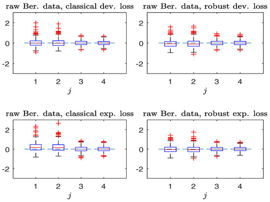
Figure 1. Simulated Bernoulli response data without contamination. Boxplots of $({\widehat{\beta }}_j-{\beta }_{j;\mathrm{o}})$, $j=1,\dots ,d$ (from left to right). (Left panels): non-robust method; (right panels): robust method.

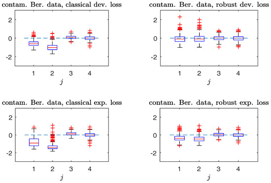
Figure 2. Simulated Bernoulli response data with contamination. The captions are identical to those in Figure 1.

For each replication, we calculate $\mathrm{MSE}\left(\widehat{\eta }\right)=n^{-1}{\sum }_{i=1}^n{\{{\widehat{\eta }}_{\widehat{\mathit{\beta }}}\left(t_i\right)-{\eta }^{\mathrm{o}}\left(t_i\right)\}}^2$. Figure 3 and Figure 4 compare the plots of ${\widehat{\eta }}_{\widehat{\mathit{\beta }}}\left(t\right)$ from typical samples, using non-robust and robust-BD estimates, where the deviance loss and exponential loss are used as the BD in the top and bottom panels, respectively. There, the typical sample in each panel is selected in a way such that its MSE value corresponds to the 50-th percentile among the MSE-ranked values from 500 replications. These fitted curves reveal little difference between using the robust and non-robust methods, in the absence of contamination. For contaminated cases, robust estimates perform slightly better than non-robust estimates. Moreover, the boundary bias issue arising from the curve estimates at the edges using the local constant method can be ameliorated by using the local-linear method.

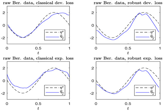
Figure 3. Simulated Bernoulli response data without contamination. Plots of ${\eta }^{\mathrm{o}}\left(t\right)$ and ${\widehat{\eta }}_{\widehat{\mathit{\beta }}}\left(t\right)$. (Left panels): non-robust method; (right panels): robust method.

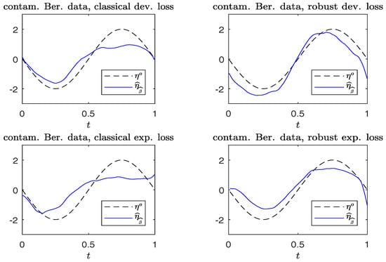
Figure 4. Simulated Bernoulli response data with contamination. Plots of ${\eta }^{\mathrm{o}}\left(t\right)$ and ${\widehat{\eta }}_{\widehat{\mathit{\beta }}}\left(t\right)$. (Left panels): non-robust method; (right panels): robust method.

6.2. Gaussian Responses

We generate independent observations ${\left\{({\mathit{X}}_i,T_i,Y_i)\right\}}_{i=1}^n$ from $(\mathit{X},T,Y)$ satisfying:

$$Y\mid (\mathit{X},T)\sim N(m(\mathit{X},T),{\sigma }^2),(\mathit{X},{\Phi }^{-1}\left(T\right))\sim N(0,\Sigma ),$$

where $\sigma =1$, $\Sigma =\left({\sigma }_{jk}\right)$ with ${\sigma }_{jk}={0.2}^{|j-k|}$, $\Phi$ denotes the CDF of the standard normal distribution. The link function is $m(\mathit{x},t)={\mathit{x}}^T{\mathit{\beta }}_{\mathrm{o}}+{\eta }^{\mathrm{o}}\left(t\right)$, where ${\mathit{\beta }}_{\mathrm{o}}={(2,-2,1,-1,0,0)}^T$ and ${\eta }^{\mathrm{o}}\left(t\right)=2\sin \left\{\pi (1+2t)\right\}$. The quadratic loss is utilized as the BD.

For each dataset simulated from the true model, a contaminated data-set is created, where 10 data points $(X_{i,j},Y_i)$ are subject to contamination. They are replaced by $(X_{i,j}^{\ast },Y_i^{\ast })$, where $Y_i^{\ast }=Y_i\mathrm{I}\left\{\right|Y_i-m({\mathit{X}}_i,T_i)|/\sigma >2\}+15\mathrm{I}\left\{\right|Y_i-m({\mathit{X}}_i,T_i)|/\sigma \le 2\}$, $i=1,\dots ,10$,

$$\begin{array}{c}{X}_{1,2}^{\ast }=5\mathrm{sign}(U_1-0.5),X_{2,2}^{\ast }=5\mathrm{sign}(U_2-0.5),X_{3,2}^{\ast }=5\mathrm{sign}(U_3-0.5),\hfill \\ X_{4,4}^{\ast }=5\mathrm{sign}(U_4-0.5),X_{5,6}^{\ast }=5\mathrm{sign}(U_5-0.5),X_{6,1}^{\ast }=5\mathrm{sign}(U_6-0.5),\hfill \\ X_{7,2}^{\ast }=5\mathrm{sign}(U_7-0.5),X_{8,3}^{\ast }=5\mathrm{sign}(U_8-0.5),X_{9,4}^{\ast }=5\mathrm{sign}(U_9-0.5),\hfill \\ X_{10,5}^{\ast }=5\mathrm{sign}(U_{10}-0.5),\hfill \end{array}$$

with $\left\{U_i\right\}\stackrel{\mathrm{i}.\mathrm{i}.\mathrm{d}.}{\sim }\mathrm{Uniform}(0,1)$.

Figure 5 and Figure 6 compare the boxplots of $({\widehat{\beta }}_j-{\beta }_{j;\mathrm{o}})$, $j=1,\dots ,d$, on the top panels, and plots of ${\widehat{\eta }}_{\widehat{\mathit{\beta }}}\left(t\right)$ from typical samples, on the bottom panels, using the non-robust and robust-BD estimates. The typical samples are selected similar to those in Section 6.1. The simulation results in Figure 5 indicate that the robust method performs, as well as the non-robust method for estimating both the parameter vector and non-parametric curve in non-contaminated cases. Figure 6 reveals that the robust estimates are less sensitive to outliers than the non-robust counterparts. Indeed, the non-robust method yields a conceivable bias for parametric estimation, and non-parametric estimation is worse than that of the robust method.

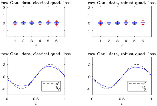
Figure 5. Simulated Gaussian response data without contamination. Top panels: boxplots of $({\widehat{\beta }}_j-{\beta }_{j;\mathrm{o}})$, $j=1,\dots ,d$ (from left to right). Bottom panels: plots of ${\eta }^{\mathrm{o}}\left(t\right)$ and ${\widehat{\eta }}_{\widehat{\mathit{\beta }}}\left(t\right)$. (Left panels): non-robust method; (right panels): robust method.

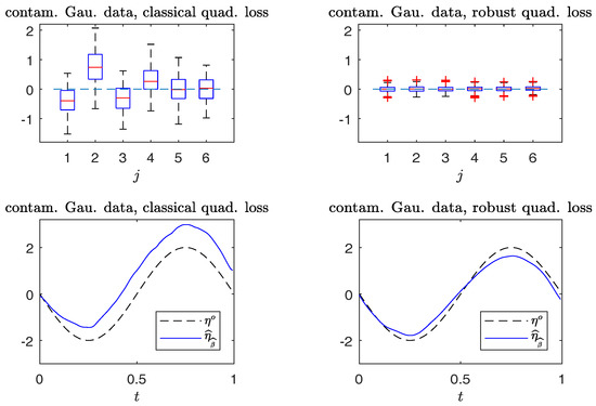
Figure 6. Simulated Gaussian response data with contamination. Top panels: boxplots of $({\widehat{\beta }}_j-{\beta }_{j;\mathrm{o}})$, $j=1,\dots ,d$ (from left to right). Bottom panels: plots of ${\eta }^{\mathrm{o}}\left(t\right)$ and ${\widehat{\eta }}_{\widehat{\mathit{\beta }}}\left(t\right)$. (Left panels): non-robust method; (right panels): robust method.

Figure 7 gives the QQ plots of the (first to 95-th) percentiles of the Wald-type statistic $W_n$ versus those of the ${\chi }_2^2$ distribution for testing the null hypothesis:

$$H_0:{\beta }_{2;\mathrm{o}}=-2\mathrm{and}{\beta }_{4;\mathrm{o}}=-1.$$

(32)

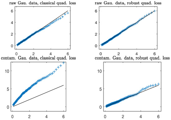
Figure 7. Simulated Gaussian response data with contamination. Empirical quantiles (on the y-axis) of the Wald-type statistics $W_n$ versus quantiles (on the x-axis) of the ${\chi }^2$ distribution. Solid line: the 45 degree reference line. (Left panels): non-robust method; (right panels): robust method.

The plots depict that in both clean and contaminated cases, the robust $W_n$ (in right panels) closely follows the ${\chi }_2^2$ distribution, lending support to Theorem 3. On the other hand, the non-robust $W_n$ agrees well with the ${\chi }_2^2$ distribution in clean data; the presence of a small number of outlying data points severely distorts the sampling distribution of the non-robust $W_n$ (in the bottom left panel) from the ${\chi }_2^2$ distribution, yielding inaccurate levels of the test.

To assess the stability of the power of the Wald-type test for testing the hypothesis (32), we evaluate the power in a sequence of alternatives with parameters ${\mathit{\beta }}_{\mathrm{o}}+\Delta \mathit{c}$ for each given $\Delta$, where $\mathit{c}={\mathit{\beta }}_{\mathrm{o}}+{(1,\dots ,1)}^T$. Figure 8 plots the empirical rejection rates of the null model in the non-contaminated case and the contaminated case. The price to pay for the robust $W_n$ is a little loss of power in the non-contaminated cases. However, under contamination, a very different behavior is observed. The observed power curve of the robust $W_n$ is close to those attained in the non-contaminated case. On the contrary, the non-robust $W_n$ is less informative, since its power curve is much lower than that of the robust $W_n$ against the alternative hypotheses with $\Delta \ne 0$, but higher than the nominal level at the null hypothesis with $\Delta =0$.

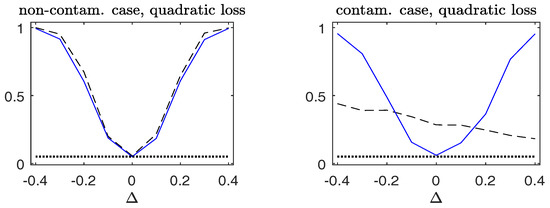
Figure 8. Observed power curves of tests for the Gaussian response data. The dashed line corresponds to the non-robust Wald-type test $W_n$; the solid line corresponds to the robust $W_n$; the dotted line indicates the 5% nominal level. (Left panels): non-contaminated case; (right panels): contaminated case.

7. Real Data Analysis

Two real datasets are analyzed. In both cases, the quadratic loss is set to be the BD, and the nonparametric function is fitted via local-linear regression method, where the bandwidth parameter is chosen to be 25% of the interval length of the variable T. Choices of the Huber $\psi$-function and weight functions are identical to those in Section 6.

7.1. Example 1

The dataset studied in [19] consists of 2447 observations on three variables, $\log \left(\mathsf{wage}\right)$, $\mathsf{age}$ and $\mathsf{education}$, for women. It is of interest to learn how wages change with years of age and years of education. It is anticipated to find an increasing regression function of $Y=\log \left(\mathsf{wage}\right)$ in $T=\mathsf{age}$ as well as in $X_1=\mathsf{education}$. We fit a partially linear model $Y=\eta \left(T\right)+{\beta }_1{X}_1+ϵ$. Profiles of the fitted nonparametric functions $\widehat{\eta }(·)$ in Figure 9 indeed exhibit the overall upward trend in $\mathsf{age}$. The coefficient estimate is ${\widehat{\beta }}_1=0.0809$ with standard error 0.0042 using the non-robust method, and is ${\widehat{\beta }}_1=0.1334$ with standard error 0.0046 by means of the robust method. It is seen that robust estimates are similar to the non-robust counterparts. Our evaluation, based on both the non-robust and robust methods, supports the predicted result in theoretical and empirical literature in socio-economical studies.

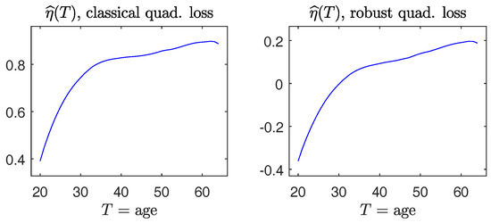
Figure 9. The dataset in [19]. (Left panels): estimate of $\eta \left(T\right)$ via the non-robust quadratic loss; (right panels): estimate of $\eta \left(T\right)$ via the robust quadratic loss.

7.2. Example 2

We analyze an employee dataset (Example 11.3 of [20]) of the Fifth National Bank of Springfield, based on year 1995 data. The bank, whose name has been changed, was charged in court with that its female employees received substantially smaller salaries than its male employees. For each of its 208 employees, the dataset consists of seven variables, $\mathsf{EducLev}$ (education level), $\mathsf{JobGrade}$ (job grade), $\mathsf{YrHired}$ (year that an employee was hired), $\mathsf{YrBorn}$ (year that an employee was born), $\mathsf{Female}$ (indicator of being female), $\mathsf{YrsPrior}$ (years of work experience at another bank before working at the Fifth National bank), and $\mathsf{Salary}$ (current annual salary in thousands of dollars).

To explain variation in salary, we fit a partial linear model, $Y=\eta \left(T\right)+{\beta }_1{X}_1+{\beta }_2{X}_2+{\beta }_3{X}_3+{\beta }_4{X}_4+{\beta }_5{X}_5+ϵ$, for $Y=\log \left(\mathsf{Salary}\right)$, $T=\mathsf{Age}$, $X_1=\mathsf{Female}$, $X_2=\mathsf{YrHired}$, $X_3=\mathsf{EducLev}$, $X_4=\mathsf{JobGrade}$ and $X_5=\mathsf{YrsPrior}$, where $\mathsf{Age}=95-\mathsf{YrBorn}$ is age. Table 1 presents parameter estimates and their standard errors (given within brackets), along with p-values calculated from the Wald-type test $W_n$. Figure 10 depicts the estimated nonparametric functions.

Table 1. Parameter estimates and p-values for partially linear model of the dataset in [20].

Variable	Classical-BD Estimation			Robust-BD Estimation
	Estimate (s.e.)		p-Value of ${\mathit{W}}_{\mathit{n}}$	Estimate (s.e.)		p-Value of ${\mathit{W}}_{\mathit{n}}$
$\mathsf{Female}$	−0.0491	(0.0232)	0.0339	0.0530	(0.0323)	0.1010
$\mathsf{YrHired}$	−0.0093	(0.0026)	0.0005	0.0359	(0.0086)	0.0000
$\mathsf{EducLev}$	0.0179	(0.0079)	0.0228	−0.0133	(0.0131)	0.3103
$\mathsf{JobGrade}$	0.0899	(0.0075)	0.0000	0.1672	(0.0168)	0.0000
$\mathsf{YrsPrior}$	0.0033	(0.0023)	0.1528	−0.0050	(0.0061)	0.4104

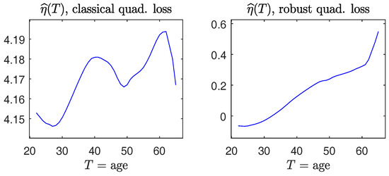
Figure 10. The dataset in [20]. (Left panel): estimate of $\eta \left(T\right)$ via the non-robust quadratic loss; (right panel): estimate of $\eta \left(T\right)$ via the robust quadratic loss.

It is interesting to note that for this dataset, results from using the robust and non-robust methods make a difference in drawing conclusions. For example, from Table 1, the non-robust method gives the estimate of parameter ${\beta }_1$ for gender to be below zero, which may be interpreted as the evidence of discrimination against female employees in salary and lends support to the plaintiff. In contrast, the robust method yields ${\widehat{\beta }}_1>0$, which does not indicate that gender has an adverse effect. (A similar conclusion made from penalized-likelihood was obtained in Section 4.1 of [21]). Moreover, the estimated nonparametric functions $\widehat{\eta }(·)$ obtained from non-robust and robust methods are qualitatively different: the former method does not deliver a monotone increasing pattern with Age, whereas the latter method does. Whether or not the difference was caused by outlying observations will be an interesting issue to be investigated.

8. Discussion

Over the past two decades, nonparametric inference procedures for testing hypotheses concerning nonparametric regression functions have been developed extensively. See [22,23,24,25,26] and the references therein. The work on the generalized likelihood ratio test [24] offers light into nonparametric inference, based on function estimation under nonparametric models, using the quadratic loss function as the error measure. These works do not directly deal with the robust procedure. Exploring the inference on nonparametric functions, such as ${\eta }^{\mathrm{o}}\left(t\right)$ in GPLM associated with a scalar variable T and the additive structure ${\sum }_{d=1}^D{\eta }_d^{\mathrm{o}}\left(t_d\right)$ as in [27] with a vector variable $\mathit{T}=(T_1,\dots ,T_D)$, estimated via the “robust-BD” as the error measure, when there are possible outlying data points, will be the future work.

This paper utilizes the class BD of loss functions, the optimal choice of which depends on specific settings and criteria. For e.g., regression and classification will utilize different loss functions, and thus further study on optimality is desirable.

Some recent work on partially linear models in econometrics includes [28,29,30]. There, the nonparametric function is approximated via linear expansions, with the number of coefficients diverging with n. Developing inference procedures to be resistant to outliers could be of interest.

References

- Andrews, D. Asymptotics for semiparametric econometric models via stochastic equicontinuity. Econometrica 1994, 62, 43–72. [Google Scholar] [CrossRef]
- Robinson, P.M. Root-n consistent semiparametric regression. Econometrica 1988, 56, 931–954. [Google Scholar] [CrossRef]
- Speckman, P. Kernel smoothing in partial linear models. J. R. Statist. Soc. B 1988, 50, 413–436. [Google Scholar]
- Yatchew, A. An elementary estimator of the partial linear model. Econ. Lett. 1997, 57, 135–143. [Google Scholar] [CrossRef]
- Fan, J.; Li, R. New estimation and model selection procedures for semiparametric modeling in longitudinal data analysis. J. Am. Stat. Assoc. 2004, 99, 710–723. [Google Scholar] [CrossRef]
- McCullagh, P.; Nelder, J.A. Generalized Linear Models, 2nd ed.; Chapman & Hall: London, UK, 1989. [Google Scholar]
- Zhang, C.M.; Yu, T. Semiparametric detection of significant activation for brain fMRI. Ann. Stat. 2008, 36, 1693–1725. [Google Scholar] [CrossRef]
- Fan, J.; Huang, T. Profile likelihood inferences on semiparametric varying-coefficient partially linear models. Bernoulli 2005, 11, 1031–1057. [Google Scholar] [CrossRef]
- Boente, G.; He, X.; Zhou, J. Robust estimates in generalized partially linear models. Ann. Stat. 2006, 34, 2856–2878. [Google Scholar] [CrossRef]
- Zhang, C.M.; Guo, X.; Cheng, C.; Zhang, Z.J. Robust-BD estimation and inference for varying-dimensional general linear models. Stat. Sin. 2014, 24, 653–673. [Google Scholar] [CrossRef]
- Fan, J.; Gijbels, I. Local Polynomial Modeling and Its Applications; Chapman and Hall: London, UK, 1996. [Google Scholar]
- Brègman, L.M. A relaxation method of finding a common point of convex sets and its application to the solution of problems in convex programming. USSR Comput. Math. Math. Phys. 1967, 7, 620–631. [Google Scholar] [CrossRef]
- Hastie, T.; Tibshirani, R.; Friedman, J. The Elements of Statistical Learning; Springer: New York, NY, USA, 2001. [Google Scholar]
- Zhang, C.M.; Jiang, Y.; Shang, Z. New aspects of Bregman divergence in regression and classification with parametric and nonparametric estimation. Can. J. Stat. 2009, 37, 119–139. [Google Scholar] [CrossRef]
- Huber, P. Robust estimation of a location parameter. Ann. Math. Statist. 1964, 35, 73–101. [Google Scholar] [CrossRef]
- Van der Vaart, A.W. Asymptotic Statistics; Cambridge University Press: Cambridge, UK, 1998. [Google Scholar]
- Friedman, J.; Hastie, T.; Tibshirani, R. Regularization paths for generalized linear models via coordinate descent. J. Stat. Softw. 2010, 33, 1–22. [Google Scholar] [CrossRef] [PubMed]
- Carroll, R.; Fan, J.; Gijbels, I.; Wand, M. Generalized partially linear single-index models. J. Am. Stat. Assoc. 1997, 92, 477–489. [Google Scholar] [CrossRef]
- Mukarjee, H.; Stern, S. Feasible nonparametric estimation of multiargument monotone functions. J. Am. Stat. Assoc. 1994, 89, 77–80. [Google Scholar] [CrossRef]
- Albright, S.C.; Winston, W.L.; Zappe, C.J. Data Analysis and Decision Making with Microsoft Excel; Duxbury Press: Pacific Grove, CA, USA, 1999. [Google Scholar]
- Fan, J.; Peng, H. Nonconcave penalized likelihood with a diverging number of parameters. Ann. Stat. 2004, 32, 928–961. [Google Scholar]
- Dette, H. A consistent test for the functional form of a regression based on a difference of variance estimators. Ann. Stat. 1999, 27, 1012–1050. [Google Scholar] [CrossRef]
- Dette, H.; von Lieres und Wilkau, C. Testing additivity by kernel-based methods. Bernoulli 2001, 7, 669–697. [Google Scholar] [CrossRef]
- Fan, J.; Zhang, C.M.; Zhang, J. Generalized likelihood ratio statistics and Wilks phenomenon. Ann. Stat. 2001, 29, 153–193. [Google Scholar] [CrossRef]
- Hong, Y.M.; Lee, Y.J. A loss function approach to model specification testing and its relative efficiency. Ann. Stat. 2013, 41, 1166–1203. [Google Scholar] [CrossRef]
- Zheng, J.X. A consistent test of functional form via nonparametric estimation techniques. J. Econ. 1996, 75, 263–289. [Google Scholar] [CrossRef]
- Opsomer, J.D.; Ruppert, D. A root-n consistent backfitting estimator for semiparametric additive modeling. J. Comput. Graph. Stat. 1999, 8, 715–732. [Google Scholar] [CrossRef]
- Belloni, A.; Chernozhukov, V.; Hansen, C. Inference on treatment effects after selection amongst high-dimensional controls. Rev. Econ. Stud. 2014, 81, 608–650. [Google Scholar] [CrossRef]
- Cattaneo, M.D.; Jansson, M.; Newey, W.K. Alternative asymptotics and the partially linear model with many regressors. Econ. Theory 2016, 1–25. [Google Scholar] [CrossRef]
- Cattaneo, M.D.; Jansson, M.; Newey, W.K. Treatment effects with many covariates and heteroskedasticity. arXiv, 2015; arXiv:1507.02493. [Google Scholar]
- Mack, Y.P.; Silverman, B.W. Weak and strong uniform consistency of kernel regression estimates. Z. Wahrsch. Verw. Gebiete 1982, 61, 405–415. [Google Scholar] [CrossRef]
© 2017 by the authors. Licensee MDPI, Basel, Switzerland. This article is an open access article distributed under the terms and conditions of the Creative Commons Attribution (CC BY) license (http://creativecommons.org/licenses/by/4.0/).