A Two-Stage Maximum Entropy Prior of Location Parameter with a Stochastic Multivariate Interval Constraint and Its Properties

Abstract

This paper proposes a two-stage maximum entropy prior to elicit uncertainty regarding a multivariate interval constraint of the location parameter of a scale mixture of normal model. Using Shannon’s entropy, this study demonstrates how the prior, obtained by using two stages of a prior hierarchy, appropriately accounts for the information regarding the stochastic constraint and suggests an objective measure of the degree of belief in the stochastic constraint. The study also verifies that the proposed prior plays the role of bridging the gap between the canonical maximum entropy prior of the parameter with no interval constraint and that with a certain multivariate interval constraint. It is shown that the two-stage maximum entropy prior belongs to the family of rectangle screened normal distributions that is conjugate for samples from a normal distribution. Some properties of the prior density, useful for developing a Bayesian inference of the parameter with the stochastic constraint, are provided. We also propose a hierarchical constrained scale mixture of normal model (HCSMN), which uses the prior density to estimate the constrained location parameter of a scale mixture of normal model and demonstrates the scope of its applicability.

1. Introduction

Suppose ${\mathit{y}}_i$’s are independent observations from a scale mixture of a p-variate normal distribution with the $p\times 1$ location parameter $\mathit{\theta }$ and known scale matrix. Then, a simple location model for the p-variate observations with ${\mathit{y}}_i\in {\mathbb{R}}^p$ is:

$${\mathit{y}}_i=\mathit{\theta }+{\mathit{ϵ}}_i,i=1,\dots ,n,$$

(1)

where the distribution of the $p\times 1$ vector variable ${\mathit{ϵ}}_i$ is $F\in \mathcal{F}$ with:

$$\begin{array}{c}\hfill \mathcal{F}=\left\{F:N_p\left(\mathbf{0},\kappa \left(\eta \right)\mathrm{\Lambda }\right),\eta \sim G\left(\eta \right)\mathrm{with}\kappa \left(\eta \right)>0,\mathrm{and}\eta >0\right\},\end{array}$$

(2)

where η is a mixing variable with the cdf $G\left(\eta \right)$ and $\kappa \left(\eta \right)$ is a suitably-chosen weight function.

Bayesian analysis of the model (1) begins with the specification of a prior distribution, which represents the information about the uncertain parameter $\mathit{\theta }$ that is combined with the joint probability distribution of ${\mathit{y}}_i$’s to yield the posterior distribution. When there are no constraints on the location parameter, then usual priors (e.g., Jeffreys invariant prior or an informative normal conjugate prior) can be used, and posterior inference can be performed without any difficulty. In some practical situations, however, we may have prior information that $\mathit{\theta }$ have a multivariate interval constraint, and thus, the value of $\mathit{\theta }$ needs to be located in a restricted space $\mathbf{C}\subset {\mathbb{R}}^p,$ where $\mathbf{C}=(\mathbf{a},\mathbf{b})$ is a p-variate interval with $\mathbf{a}={(a_1,\dots ,a_p)}^{\top }$ and $\mathbf{b}={(b_1,\dots ,b_p)}^{\top }.$ For the remainder of this paper, we use $\mathit{\theta }\in \mathbf{C}$ to denote the multivariate interval constraint:

$$\left\{\mathit{\theta };a_i\le {\theta }_i\le b_i,i=1,\dots ,p\right\},\mathrm{where}\mathit{\theta }={({\theta }_1,\dots ,{\theta }_p)}^{\top }.$$

(3)

When we have sufficient evidence that the constraint condition on the model (1) is true, then a suitable restriction on the parameter space, such as using a truncated prior distribution, is expected. See, e.g., [1,2,3,4], for various applications of the truncated prior distribution in Bayesian inference. However, it is often the case that prior information about the constraint is not certain for Bayesian inference. Further, even the observations from the assumed model (1) often do not provide strong evidence that the constraint is true and, therefore, may appear to contradict the assumption of the model associated with the constraint. In this case, it is expected that the uncertainty about the constraint is taken into account in eliciting a prior distribution of $\mathit{\theta }.$ When the parameter constraint is not certain for Bayesian estimation in the univariate normal location model, the seminal work by [5] proposed the use of a two-stage hierarchical prior distribution by constructing a family of skew densities based on the positively-truncated normal prior distribution. Generalizing the framework of the prior hierarchy proposed by [5,6,7,8,9,10], among others, various priors were considered for the Bayesian estimation of normal and scale mixture of normal models with uncertain interval constraints. In particular, [7] obtained the prior of $\mathit{\theta }$ as the normal selection distribution (see, e.g., [11]) and, thus, exploited the class of weighted normal distribution by [12] for reflecting the uncertain prior belief on $\mathit{\theta }.$ On the other hand, there are situations to set up a prior density of $\mathit{\theta }$ on the basis of information regarding the moments of the density, such as the mean and covariance matrix. A useful method of dealing with this situation is through the concept of entropy by [13,14]. Other general references where moment inequality constraints have been considered include [15,16]. To the best of our knowledge, however, a formal method to set up a prior density of $\mathit{\theta },$ consistent with information regarding the moments of the density, as well as the uncertain prior belief on the location parameter, has not previously been investigated in the literature. Thus, such practical considerations motivate us to develop a prior density of $\mathit{\theta },$ which is tackled in this paper.

As discussed by [17,18,19,20], the entropy has a direct relationship to information theory and measures the amount of uncertainty inherent in the probability distribution. Using this property of the entropy, we propose a two-stage hierarchical method for setting up the two-stage maximum entropy prior density of $\mathit{\theta }.$ The method will enable us to elicit information regarding the moments of the prior distribution, as well as the degree of belief in the constraint $\mathit{\theta }\in \mathbf{C}.$ Furthermore, this paper also suggests an objective method to measure the degree of belief regarding the multivariate interval constraint accounted for by using the prior. We also propose a simple way of controlling the degree of belief regarding the constraint of $\mathit{\theta }$ in Bayesian inference. This is done by investigating the relation between the degree of belief and the enrichment of the hyper-parameters of the prior density. In this respect, the study concerning the two-stage maximum entropy prior is interesting both from a theoretical and an applied point of view. On the theoretical side, it develops yet another conjugate prior of constrained $\mathit{\theta }$ based on the maximum entropy approach. The study provides several properties of the proposed prior, which advocate the idea of two stages of a prior hierarchy to elicit information regarding the moments of the prior and the stochastic constraint of $\mathit{\theta }.$ From the applied view point, the prior is especially useful for a Bayesian subjective methodology for inequality constrained multivariate linear models.

The remainder of this paper is arranged as follows. In Section 2, we propose the two-stage maximum entropy prior of $\mathit{\theta }$ by applying Boltzmann’s maximum entropy theorem (see, e.g., [21,22]) to the frame of the two-stage prior hierarchy by [5]. We also suggest an objective measure of uncertainty regarding the stochastic constraint of $\mathit{\theta }$ that is accounted for by the two-stage maximum entropy prior. In Section 3, we briefly discuss the properties of the proposed prior of $\mathit{\theta },$ which will be useful for the Bayesian analysis of $\mathit{\theta }$ subject to uncertainty regarding the multivariate interval constraint $\mathit{\theta }\in \mathbf{C}$. Section 4 provides a hierarchical scale mixture of normal model of Equation (1) using the two-stage prior, referred to as the hierarchical constrained scale mixture of normal model (HCSMN). Section 4 explores the Bayesian estimation model (1) by deriving the posterior distributions of the unknown parameters under the HCSMN and discusses the properties of the proposed measure of uncertainty that can be explained in the context of the HCSMN. In Section 5, we compare the empirical performance of the proposed prior based on synthetic data and real data applications with the HCSMN models for the estimation of $\mathit{\theta }$ with a stochastic multivariate interval constraint. Finally, the concluding remarks along with a discussion are provided in Section 6.

2. Two-Stage Maximum Entropy Prior

2.1. Maximum Entropy Prior

Sometimes, we have a situation in which partial prior information is available, outside of which it is desirable to use a prior that is as non-informative as possible. Assume that we can specify the partial information concerning $\mathit{\theta }$ in Equation (1) with continuous space $\mathrm{\Theta }.$ That is:

$$E\left[t_j\left(\mathit{\theta }\right)\right]={\int }_{\mathrm{\Theta }}^{}{t}_j\left(\mathit{\theta }\right)\pi \left(\mathit{\theta }\right)d\mathit{\theta }=t_j,j=1,\dots ,k.$$

(4)

The maximum entropy prior can be obtained by choosing $\pi \left(\mathit{\theta }\right)$ that maximizes the entropy:

$$\xi \left(\pi \right)=-{\int }_{\mathrm{\Theta }}^{}\pi \left(\mathit{\theta }\right)log\pi \left(\mathit{\theta }\right)d\mathit{\theta },$$

in the presence of the partial information in the form of Equation (4). A straightforward application of the calculus of variation leads us to the following theorem.

Lemma 1. 

(Boltzmann’s maximum entropy theorem): The density $\pi \left(\mathit{\theta }\right)$ that maximizes $\xi \left(\pi \right)$, subject to the constraints $E\left[t_j\left(\mathit{\theta }\right)\right]=t_j,$ $j=1,\dots ,k,$ takes the k-parameter exponential family form:

$${\pi }_{max}\left(\mathit{\theta }\right)\propto exp\left\{{\lambda }_1{t}_1\left(\mathit{\theta }\right)+{\lambda }_2{t}_2\left(\mathit{\theta }\right)\cdots +{\lambda }_k{t}_k\left(\mathit{\theta }\right)\right\},\mathit{\theta }\in \mathrm{\Theta },$$

(5)

where ${\lambda }_1,{\lambda }_2,\dots ,{\lambda }_k$ can be determined, via the k-constraints, in terms of $t_1,$ …, $t_k.$

Proof. 

See, [22] for the proof. ☐

When the partial information is about the mean and covariance matrix of $\mathit{\theta },$ outside of which it is desired to use a prior that is as non-informative as possible, then the theorem yields the following result.

Corollary 1. 

As partial prior information, let the parameter $\mathit{\theta }={({\theta }_1,\dots ,{\theta }_p)}^{\top }$ have a probability distribution on ${\mathbb{R}}^p$ with mean vector ${\mathit{\theta }}_0={({\theta }_{01},\dots ,{\theta }_{0p})}^{\top }$ and covariance matrix $\mathrm{\Sigma },$ then the maximum entropy prior of $\mathit{\theta }$ is:

$${\pi }_{max}\left(\mathit{\theta }\right)={\left(2\pi \right)}^{-p/2}{\left|\mathrm{\Sigma }\right|}^{-1/2}exp\left\{-\frac{1}{2}{(\mathit{\theta }-{\mathit{\theta }}_0)}^{\top }{\mathrm{\Sigma }}^{-1}(\mathit{\theta }-{\mathit{\theta }}_0)\right\},\mathit{\theta }\in {\mathbb{R}}^p,$$

(6)

a density of the $N_p({\mathit{\theta }}_0,\mathrm{\Sigma })$ distribution.

Proof. 

According to Lemma 1, the partial information gives $t_j\left(\mathit{\theta }\right)={\theta }_j$ and $t_j={\theta }_{0j}$ for $j=1,\dots ,p,$ $t_{p+1}\left(\mathit{\theta }\right)=\mathrm{tr}\left[{\mathrm{\Sigma }}^{-1}(\mathit{\theta }-{\mathit{\theta }}_0){(\mathit{\theta }-{\mathit{\theta }}_0)}^{\top }\right]$ and $t_{p+1}=p.$ ${\int }_{{\mathbb{R}}^p}{\pi }_{max}\left(\mathit{\theta }\right)d\mathit{\theta }=1$ requires ${\lambda }_1=\cdots ={\lambda }_p=0$ and ${\lambda }_{p+1}<0.$ Thus, the density ${\pi }_{max}\left(\mathit{\theta }\right)$ is proportional to $exp\left\{-{\lambda }_{p+1}\mathrm{tr}\left[{\mathrm{\Sigma }}^{-1}(\mathit{\theta }-{\mathit{\theta }}_0){(\mathit{\theta }-{\mathit{\theta }}_0)}^{\top }\right]\right\}.$ Setting ${\lambda }_{p+1}=-t_{p+1}/2p$ and obtaining the normalizing constant, then we see that the maximum entropy prior of the parameter in Equation (1) is Equation (6). ☐

In practical situations, we sometimes have partial information about a multivariate interval constraint (i.e., $\mathit{\theta }\in \mathbf{C}$) in addition to the first two moments as given in Corollary 1.

Corollary 2. 

Assume that the prior distribution of $\mathit{\theta }={({\theta }_1,\dots ,{\theta }_p)}^{\top }$ has the mean vector ${\mathit{\theta }}_0={({\theta }_{01},\dots ,{\theta }_{0p})}^{\top }$ and covariance matrix $\mathrm{\Sigma }.$ Further assume, a priori, that the space of $\mathit{\theta }$ is constrained to a multivariate interval, $\{\mathit{\theta };\mathit{\theta }\in \mathbf{C}\}$ given in Equation (3). Then, a constrained maximum entropy prior of $\mathit{\theta }$ is given by:

$${\pi }_{const}\left(\mathit{\theta }\right)=\frac{{\left(2\pi \right)}^{-p/2}{\left|\mathrm{\Sigma }\right|}^{-1/2}exp\left\{-\frac{1}{2}{(\mathit{\theta }-{\mathit{\theta }}_0)}^{\top }{\mathrm{\Sigma }}^{-1}(\mathit{\theta }-{\mathit{\theta }}_0)\right\}}{Pr(\mathit{\theta }\in \mathbf{C})},\mathit{\theta }\in \mathbf{C},$$

(7)

a density of the $N_p({\mathit{\theta }}_0,\mathrm{\Sigma })I(\mathit{\theta }\in \mathbf{C})$ distribution, which is a p-dimensional truncated $N_p({\mathit{\theta }}_0,\mathrm{\Sigma })$ distribution with the space $\mathbf{C}.$

Proof. 

The certain multivariate interval constraint, $Pr(\mathit{\theta }\in \mathbf{C})=1,$ can be expressed in terms of moment, $E\left[I\right(\mathit{\theta }\in \mathbf{C}\left)\right]=1.$ Upon applying Lemma 1 with $t_j\left(\mathit{\theta }\right)={\theta }_j$ and $t_j={\theta }_{0j}$ for $j=1,\dots ,p,$ $t_{p+1}\left(\mathit{\theta }\right)=\mathrm{tr}\left[{\mathrm{\Sigma }}^{-1}(\mathit{\theta }-{\mathit{\theta }}_0){(\mathit{\theta }-{\mathit{\theta }}_0)}^{\top }\right]$ and $t_{p+1}=p,$ $t_{p+2}\left(\mathit{\theta }\right)=I(\mathit{\theta }\in \mathbf{C})$ and $t_{p+2}=1,$ and ${\int }_{\mathbf{C}}{\pi }_{const}\left(\mathit{\theta }\right)d\mathit{\theta }=1,$ we see that ${\lambda }_1=\cdots ={\lambda }_p=0,$ ${\lambda }_{p+1}<0,$ ${\lambda }_{p+2}=1,$ and ${\pi }_{const}\left(\mathit{\theta }\right)\propto exp\left\{-{\lambda }_{p+1}\mathrm{tr}\left[{\mathrm{\Sigma }}^{-1}(\mathit{\theta }-{\mathit{\theta }}_0){(\mathit{\theta }-{\mathit{\theta }}_0)}^{\top }\right]\right\}.$ Setting ${\lambda }_{p+1}=-1/2$, and obtaining the normalizing constant, we obtain Equation (7). ☐

2.2. Two-Stage Maximum Entropy Prior

This subsection considers the case where the maximum entropy prior of $\mathit{\theta }$ has stochastic constraint in the form of a multivariate interval, i.e., Pr$(\mathit{\theta }\in \mathbf{C})=\gamma ,$ where $\mathbf{C}$ is defined by Equation (3) and $\gamma \in [{\gamma }_{max},1].$ Here, ${\gamma }_{max}$ is Pr$(\mathit{\theta }\in \mathbf{C})$ calculated by using the maximum entropy prior distribution in Equation (6). We develop a two-stage prior of $\mathit{\theta }$, denoted by ${\pi }_{two}\left(\mathit{\theta }\right)$, which has a different formula according to the degree of belief, $\gamma ,$ regarding the constraint.

Suppose we have only partial information about the covariance matrix, ${\mathrm{\Omega }}_2,$ of the parameter $\mathit{\theta },$ in the first stage of a prior elicitation. Then, for a given mean vector ${\mathit{\mu }}_0$, we may construct the maximum entropy prior, Equation (6), so that the first stage maximum entropy prior will be ${\pi }_{max}\left(\mathit{\theta }\right|{\mathit{\mu }}_0)$, which is the density of the $N_p({\mathit{\mu }}_0,{\mathrm{\Omega }}_2)$ distribution. In addition to the information, suppose we have collected prior information about the unknown ${\mathit{\mu }}_0$, which gives a value of the mean vector ${\mathit{\theta }}_0$ and covariance matrix ${\mathrm{\Omega }}_1$, as well as a stochastic (or certain) constraint, indicating Pr$({\mathit{\mu }}_0\in \mathbf{C})=1.$ Then, in the second stage of the prior elicitation, one can elicit the additional prior partial information by using the constrained maximum entropy prior in Equation (7).

Analogous to the work of [5], we can specify all of the partial information about $\mathit{\theta }$ by following two stages of the maximum entropy prior hierarchy over $\mathit{\theta }\in {\mathbb{R}}^p:$

$$\begin{array}{ccc}\hfill {\pi }_{max}\left(\mathit{\theta }\right|{\mathit{\mu }}_0)& =& {\varphi }_p({\mathit{\mu }}_0,{\mathrm{\Omega }}_2),\hfill \end{array}$$

(8)

$$\begin{array}{ccc}\hfill {\pi }_{const}\left({\mathit{\mu }}_0\right)& =& {\varphi }_p({\mathit{\theta }}_0,{\mathrm{\Omega }}_1)\mathrm{I}({\mathit{\mu }}_0\in \mathbf{C}),\hfill \end{array}$$

(9)

where ${\varphi }_p({\mathit{\theta }}_0,{\mathrm{\Omega }}_1)\mathrm{I}({\mathit{\mu }}_0\in \mathbf{C})$ is a truncated normal density, i.e., the density of the $N_p({\mathit{\theta }}_0,{\mathrm{\Omega }}_1)\mathrm{I}({\mathit{\mu }}_0\in \mathbf{C})$ variate, and ${\mathrm{\Omega }}_1+{\mathrm{\Omega }}_2=\mathrm{\Sigma }.$ Thus, the two stages of prior hierarchy are as follows. In the first stage, given ${\mathit{\mu }}_0,$ $\mathit{\theta }$ has a maximum entropy prior that is the $N_p({\mathit{\mu }}_0,{\mathrm{\Omega }}_2)$ distribution as in Equation (6). In the second stage, ${\mathit{\mu }}_0$ has a distribution obtained by truncating the maximum entropy prior distribution to elicit uncertainty about the prior information that $\mathit{\theta }\in \mathbf{C}.$ It may be sensible to assume that the value of ${\mathit{\theta }}_0$ is located in the multivariate interval $\mathbf{C}$ or in the centroid of the interval.

Definition 1. 

The marginal prior density of $\mathit{\theta }$, obtained from the two stages of the maximum entropy prior hierarchy Equations (8) and (9), is called as a two-stage maximum entropy prior of $\mathit{\theta }$.

Since ${\mathrm{\Omega }}_1+{\mathrm{\Omega }}_2=\mathrm{\Sigma },$ if the constraint is completely certain (i.e., $\gamma =1$), we may set ${\mathrm{\Omega }}_2\to \mathbf{O}$ to get the ${\pi }_{const}\left(\mathit{\theta }\right)$ from the two stages of maximum entropy prior, while the two-stage prior yields ${\pi }_{max}\left(\mathit{\theta }\right)$ with $\gamma ={\gamma }_{max}$ for the case where ${\mathrm{\Omega }}_1=\mathbf{O}.$ Thus, the hyper-parameters ${\mathrm{\Omega }}_1$ and ${\mathrm{\Omega }}_2$ may need to be assessed to achieve the degree of belief γ about the stochastic constraint. When ${\mathrm{\Omega }}_1\ne \mathbf{O}$ and ${\mathrm{\Omega }}_2\ne \mathbf{O},$ the above hierarchy of priors yields the following marginal prior of $\mathit{\theta }.$

Lemma 2. 

The two stages of the prior hierarchy of Equations (8) and (9) yield the two-stage maximum entropy prior distribution of $\mathit{\theta }$ given by:

$$\begin{array}{ccc}\hfill {\pi }_{two}\left(\mathit{\theta }\right)& =& \frac{{\varphi }_p(\mathit{\theta };{\mathit{\theta }}_0,\mathrm{\Sigma }){\overline{\mathrm{\Phi }}}_p(\mathbf{C};\mathit{\mu },Q)}{{\overline{\mathrm{\Phi }}}_p(\mathbf{C};{\mathit{\theta }}_0,{\mathrm{\Omega }}_1)},\mathit{\theta }\in {\mathbb{R}}^p\hfill \end{array}$$

(10)

where ${\varphi }_p(\mathbf{x};\mathbf{c},\mathbf{A})$ denotes the pdf of $\mathbf{X}\sim N_p(\mathbf{c},\mathbf{A})$ and ${\overline{\mathrm{\Phi }}}_p(\mathbf{C};\mathbf{c},\mathbf{A})$ denotes a p-dimensional rectangle probability of the distribution of $\mathbf{X}$, i.e., $P(\mathbf{X}\in \mathbf{C}),$ $\mathit{\mu }={\mathit{\theta }}_0+{\mathrm{\Omega }}_1{\mathrm{\Sigma }}^{-1}(\mathit{\theta }-{\mathit{\theta }}_0),$ $\mathrm{\Sigma }={\mathrm{\Omega }}_1+{\mathrm{\Omega }}_2$ and $Q={({\mathrm{\Omega }}_1^{-1}+{\mathrm{\Omega }}_2^{-1})}^{-1}.$

Proof. 

$$\begin{array}{ccc}\hfill {\pi }_{two}\left(\mathit{\theta }\right)& =& \frac{{\int }_{{\mathit{\mu }}_0\in \mathbf{C}}{\varphi }_p(\mathit{\theta };{\mathit{\mu }}_0,{\mathrm{\Omega }}_2){\varphi }_p({\mathit{\mu }}_0;{\mathit{\theta }}_0,{\mathrm{\Omega }}_1)d{\mathit{\mu }}_0}{Pr({\mathit{\mu }}_0\in \mathbf{C})},\hfill \\ & =& \frac{{\varphi }_p(\mathit{\theta };{\mathit{\theta }}_0,\mathrm{\Sigma }){\int }_{{\mathit{\mu }}_0\in \mathbf{C}}{\varphi }_p({\mathit{\mu }}_0;\mathit{\mu },Q)d{\mathit{\mu }}_0}{{\overline{\mathrm{\Phi }}}_p(\mathbf{C};{\mathit{\theta }}_0,{\mathrm{\Omega }}_1)},\hfill \end{array}$$

because $\mathit{\mu }={\mathit{\theta }}_0+{\mathrm{\Omega }}_1{\mathrm{\Sigma }}^{-1}(\mathit{\theta }-{\mathit{\theta }}_0)=\mathit{\theta }+{\mathrm{\Omega }}_2{\mathrm{\Sigma }}^{-1}({\mathit{\theta }}_0-\mathit{\theta })$ and ${\mathit{\theta }}^{\top }{\mathrm{\Omega }}_2^{-1}\mathit{\theta }+{\mathit{\theta }}_0^{\top }{\mathrm{\Omega }}_1^{-1}{\mathit{\theta }}_0-{\mathit{\mu }}^{\top }\left({\mathrm{\Omega }}_2^{-1}\mathit{\theta }+{\mathrm{\Omega }}_1^{-1}{\mathit{\theta }}_0\right)={(\mathit{\theta }-{\mathit{\theta }}_0)}^{\top }{\mathrm{\Sigma }}^{-1}(\mathit{\theta }-{\mathit{\theta }}_0).$ ☐

In fact, the density ${\pi }_{two}\left(\mathit{\theta }\right)$ belongs to the family of rectangle screened multivariate normal ($RSN$) distributions studied by [23].

Corollary 3. 

The distribution law of $\mathit{\theta }$ with the density in Equation (10) is:

$$\begin{array}{ccc}\hfill \mathit{\theta }& \stackrel{d}{=}& \left[{\mathbf{X}}_2|{\mathbf{X}}_1\in \mathbf{C}\right]\sim RS{N}_p(\mathbf{C};\mathbf{\tau },\mathrm{\Psi }),\hfill \end{array}$$

(11)

which is a p-dimensional $RSN$ distribution with respective location and scale parameters $\mathit{\tau }$ and Ψ and the rectangle screening space $\mathbf{C}.$ Here, the joint distribution of ${\mathbf{X}}_1$ and ${\mathbf{X}}_2$ is $N_{2p}(\mathit{\tau },\mathrm{\Psi }),$ where $\mathit{\tau }={({\mathit{\theta }}_0^{\top },{\mathit{\theta }}_0^{\top })}^{\top }$ and $\mathrm{\Psi }=\left(\begin{array}{cc}{\mathrm{\Omega }}_1& {\mathrm{\Omega }}_1\\ {\mathrm{\Omega }}_1& \mathrm{\Sigma }\end{array}\right)$.

Proof. 

The density of $\left[{\mathbf{X}}_2\right|{\mathbf{X}}_1\in \mathbf{C}]$ is:

$$\begin{array}{ccc}\hfill {\pi }_{two}\left({\mathit{x}}_2\right)& =& \frac{{\varphi }_p\left({\mathit{x}}_2;{\mathit{\theta }}_0,\mathrm{\Sigma }\right){\int }_{\mathbf{C}}^{}{\varphi }_p\left({\mathit{x}}_1;{\mathit{\mu }}_{{\mathit{x}}_1|{\mathit{x}}_2},{\mathrm{\Omega }}_{{\mathit{x}}_1|{\mathit{x}}_2}\right)d{\mathit{x}}_1}{{\int }_{\mathbf{C}}^{}{\varphi }_p\left({\mathit{x}}_1;{\mathit{\theta }}_0,{\mathrm{\Omega }}_1\right)d{\mathit{x}}_1}\hfill \\ & =& \frac{{\varphi }_p\left({\mathit{x}}_2;{\mathit{\theta }}_0,\mathrm{\Sigma }\right){\overline{\mathrm{\Phi }}}_p\left(\mathbf{C};{\mathit{\mu }}_{{\mathit{x}}_1|{\mathit{x}}_2},{\mathrm{\Omega }}_{{\mathit{x}}_1|{\mathit{x}}_2}\right)}{{\overline{\mathrm{\Phi }}}_p\left(\mathbf{C};{\mathit{\theta }}_0,{\mathrm{\Omega }}_1\right)}\hfill \end{array}$$

where ${\mathit{\mu }}_{{\mathit{x}}_1|{\mathit{x}}_2}={\mathit{\theta }}_0+{\mathrm{\Omega }}_1{\mathrm{\Sigma }}^{-1}({\mathit{x}}_2-{\mathit{\theta }}_0)$ and ${\mathrm{\Omega }}_{{\mathit{x}}_1|{\mathit{x}}_2}={\mathrm{\Omega }}_1-{\mathrm{\Omega }}_1{\mathrm{\Sigma }}^{-1}{\mathrm{\Omega }}_1.$ By use of the binomial inverse theorem (see, e.g., [24] p. 23), one can easily see that ${\mathit{\mu }}_{{\mathit{x}}_1|{\mathit{x}}_2}$ and ${\mathrm{\Omega }}_{{\mathit{x}}_1|{\mathit{x}}_2}$ are respectively equivalent to $\mathit{\mu }$ and $Q,$ in Equation (10), provided that ${\mathit{x}}_2$ is changed to $\mathit{\theta }.$ ☐

According to [23], we see that the stochastic representation for the $RSN$ vector $\mathit{\theta }\sim RS{N}_p(\mathbf{C};\mathit{\tau },\mathrm{\Psi })$ is:

$$\begin{array}{ccc}\hfill \mathit{\theta }& \stackrel{d}{=}& {\mathit{\theta }}_0+{\mathbf{Y}}_1^{(\mathit{\alpha },\mathit{\beta })}+{\mathbf{Y}}_2,\hfill \end{array}$$

(12)

where ${\mathbf{Y}}_1\sim N_p(\mathbf{0},{\mathrm{\Omega }}_1)$ and ${\mathbf{Y}}_2\sim N_p(\mathbf{0},{\mathrm{\Omega }}_2)$ are independent random vectors. Here, ${\mathbf{Y}}_1^{(\mathit{\alpha },\mathit{\beta })}$ denotes a doubly-truncated multivariate normal random vector whose distribution is defined by ${\mathbf{Y}}_1^{(\mathit{\alpha },\mathit{\beta })}\stackrel{d}{=}\left[{\mathbf{Y}}_1\right|{\mathbf{Y}}_1\in (\mathit{\alpha },\mathit{\beta })]$ with $\mathit{\alpha }=\mathbf{a}-{\mathit{\theta }}_0$ and $\mathit{\beta }=\mathbf{b}-{\mathit{\theta }}_0.$ This representation enables us to implement a one-for-one method for generating a random vector with the $RS{N}_p(\mathbf{C},\mathit{\tau },\mathrm{\Psi })$ distribution. For generating the doubly-truncated multivariate normal vector ${\mathbf{Y}}_1^{(\mathit{\alpha },\mathit{\beta })},$ the R package tmvtnorm by [25] can be used, where R is a computer language and an environment for statistical computing and graphics.

2.3. Entropy of a Maximum Entropy Prior

Suppose we have partial a priori information that we can specify values for the covariance matrices ${\mathrm{\Omega }}_1$ and ${\mathrm{\Omega }}_2,$ where $\mathrm{\Sigma }={\mathrm{\Omega }}_1+{\mathrm{\Omega }}_2.$

2.3.1. Case 1: Two-stage Maximum Entropy Prior

When the two-stage maximum entropy prior ${\pi }_{two}\left(\mathit{\theta }\right)$ is assumed for the prior distribution of $\mathit{\theta },$ its entropy is given by:

$$\begin{array}{ccc}\hfill Ent\left({\pi }_{two}\left(\mathit{\theta }\right)\right)& =& -{\int }_{{\mathbb{R}}^p}{\pi }_{two}\left(\mathit{\theta }\right)log{\pi }_{two}\left(\mathit{\theta }\right)d\mathit{\theta }\hfill \\ & =& \frac{p}{2}log\left(2\pi \right)+log{\overline{\mathrm{\Phi }}}_p(\mathbf{C};{\mathit{\theta }}_0,{\mathrm{\Omega }}_1)+\frac{1}{2}\mathrm{tr}\left[{\mathrm{\Sigma }}^{-1}{E}_{two}\left[(\mathit{\theta }-{\mathit{\theta }}_0){(\mathit{\theta }-{\mathit{\theta }}_0)}^{\top }\right]\right]\hfill \\ & +& \frac{1}{2}log\left|\mathrm{\Sigma }\right|-E_{two}\left[logh\left(\mathit{\theta }\right)\right],\hfill \end{array}$$

(13)

where $\mathrm{\Sigma }={\mathrm{\Omega }}_1+{\mathrm{\Omega }}_2,$ $h\left(\mathit{\theta }\right)={\overline{\mathrm{\Phi }}}_p\left(\mathbf{C};{\mathit{\theta }}_0+{\mathrm{\Omega }}_1^{\top }{\mathrm{\Sigma }}^{-1}(\mathit{\theta }-{\mathit{\theta }}_0),{\mathrm{\Omega }}_1-{\mathrm{\Omega }}_1^{\top }{\mathrm{\Sigma }}^{-1}{\mathrm{\Omega }}_1\right),$ and the $E_{two}$ denotes the expectation with respect to the $RSN$ distribution with the density ${\pi }_{two}\left(\mathit{\theta }\right).$ Equation (12) shows that $E\left[\mathit{\theta }\right]={\mathit{\theta }}_0+\mathit{\xi },$ and $Cov\left(\mathit{\theta }\right)={\mathrm{\Omega }}_2+H.$ Here, $\mathit{\xi }={({\xi }_1,\dots ,{\xi }_p)}^{\top }$ and $H=\left\{h_{ij}\right\},$ $i,j=1,\dots ,p,$ are the mean vector and covariance matrix of the doubly-truncated multivariate normal random vector, ${\mathbf{Y}}_1\sim N_p\left(\mathbf{0},{\mathrm{\Omega }}_1\right)\mathrm{I}\left({\mathbf{y}}_1\in (\mathit{\alpha },\mathit{\beta })\right)$. Readers are referred to [25] with the R package tmvtnorm and [26] with the R package mvtnorm for implementing the respective calculations of doubly-truncated moments and integrations. As seen in Equation (13), an analytic calculation of $E\left[logh\left(\mathit{\theta }\right)\right]$ involves a complicated integration. Instead, by using a Monte Carlo integration, we may calculate it approximately. According to Equation (12), it follows that the stochastic representation of the prior distribution $\mathit{\theta }\sim RS{N}_p(\mathbf{C};\mathit{\tau },\mathrm{\Psi })$ with density ${\pi }_{two}\left(\mathit{\theta }\right)$ is useful for generating $\mathit{\theta }$’s from the prior distribution $\mathit{\theta }$ by using the R packages mvtnorm and tmvtnorm and, hence, implementing the Monte Carlo integration.

2.3.2. Case 2: Constrained Maximum Entropy Prior

When the constrained maximum entropy prior ${\pi }_{const}\left(\mathit{\theta }\right)$ in Equation (7) is assumed for the prior distribution of $\mathit{\theta },$ its entropy is given by:

$$\begin{array}{ccc}\hfill Ent\left({\pi }_{const}\left(\mathit{\theta }\right)\right)& =& -{\int }_{\mathbf{C}}{\pi }_{const}\left(\mathit{\theta }\right)log{\pi }_{const}\left(\mathit{\theta }\right)d\mathit{\theta }\hfill \\ & =& \frac{p}{2}log\left(2\pi \right)+log{\overline{\mathrm{\Phi }}}_p(\mathbf{C};{\mathit{\theta }}_0,\mathrm{\Sigma })+\frac{1}{2}log\left|\mathrm{\Sigma }\right|\hfill \\ & +& \frac{1}{2}\mathrm{tr}\left({\mathrm{\Sigma }}^{-1}{E}_{const}\left[(\mathit{\theta }-{\mathit{\theta }}_0){(\mathit{\theta }-{\mathit{\theta }}_0)}^{\top }\right]\right).\hfill \end{array}$$

The $E_{const}$ denotes the expectation with respect to the doubly-truncated multivariate normal distribution with the density ${\pi }_{const}\left(\mathit{\theta }\right)$, and its analytic calculation is not possible. Instead, the R packages tmvtnorm and mvtnorm are available for calculating the respective moment and integration in the expression of $Ent\left({\pi }_{const}\right).$

2.3.3. Case 3: Maximum Entropy Prior

On the other hand, if the maximum entropy prior ${\pi }_{max}\left(\mathit{\theta }\right)$ is assumed for the prior distribution of the location parameter $\mathit{\theta },$ its entropy is given by:

$$\begin{array}{ccc}\hfill Ent\left({\pi }_{max}\left(\mathit{\theta }\right)\right)& =& -{\int }_{{\mathbb{R}}^p}{\pi }_{max}\left(\mathit{\theta }\right)log{\pi }_{max}\left(\mathit{\theta }\right)d\mathit{\theta }\hfill \\ & =& \frac{p}{2}+\frac{p}{2}log\left(2\pi \right)+\frac{1}{2}log\left|\mathrm{\Sigma }\right|.\hfill \end{array}$$

The following theorem asserts the relationship among the degrees of belief, accounted for by the three priors, about the a priori uncertain constraint $\left\{\mathit{\theta };\mathit{\theta }\in \mathbf{C}\right\}.$

Theorem 1. 

The degrees of belief ${\gamma }_{max},$ ${\gamma }_{two},$ and ${\gamma }_{const}$ about the a priori constraint $\left\{\mathit{\theta };\mathit{\theta }\in \mathbf{C}\right\},$ accounted for by ${\pi }_{max}\left(\mathit{\theta }\right),$ ${\pi }_{two}\left(\mathit{\theta }\right)$ and ${\pi }_{const}\left(\mathit{\theta }\right)$, have the following relation:

$$\begin{array}{ccc}\hfill {\gamma }_{max}& \le & {\gamma }_{two}\le {\gamma }_{const},\hfill \end{array}$$

(14)

provided that the parameters of ${\pi }_{two}\left(\mathit{\theta }\right)$ in Equation (10) satisfy:

$${\overline{\mathrm{\Phi }}}_{2p}\left({\mathbf{C}}^{*};\mathit{\tau },\mathrm{\Psi }\right)\ge {\overline{\mathrm{\Phi }}}_p\left(\mathbf{C};{\mathit{\theta }}_0,{\mathrm{\Omega }}_1\right){\overline{\mathrm{\Phi }}}_p\left(\mathbf{C};{\mathit{\theta }}_0,\mathrm{\Sigma }\right),$$

where ${\mathbf{C}}^{*}=\{\mathit{x};{\mathit{x}}_1\in \mathbf{C},{\mathit{x}}_2\in \mathbf{C}\}$ denotes the $2p$-variate interval of random vector $\mathbf{X}={({\mathbf{X}}_1^{\top },{\mathbf{X}}_2^{\top })}^{\top },$ the equality ${\gamma }_{max}={\gamma }_{two}$ holds for ${\mathrm{\Omega }}_1=\mathbf{O},$ ${\gamma }_{two}={\gamma }_{const}$ holds for ${\mathrm{\Omega }}_2=\mathbf{O}$ and ${\gamma }_{max}={\gamma }_{two}={\gamma }_{const}$ holds for $\mathbf{C}={\mathbb{R}}^p.$

Proof. 

The conditions for equalities are straightforward from the stochastic representation in Equation (12). Under the ${\pi }_{max}\left(\mathit{\theta }\right)$ in Equation (6),

$${\gamma }_{max}=Pr(\mathit{\theta }\in \mathbf{C})={\overline{\mathrm{\Phi }}}_p(\mathbf{C};{\mathit{\theta }}_0,\mathrm{\Sigma }),{\gamma }_{two}={\int }_{\mathit{\theta }\in \mathbf{C}}{\pi }_{two}\left(\mathit{\theta }\right)d\mathit{\theta }=\frac{{\overline{\mathrm{\Phi }}}_{2p}\left({\mathbf{C}}^{*};\mathit{\tau },\mathrm{\Psi }\right)}{{\overline{\mathrm{\Phi }}}_p\left(\mathbf{C};{\mathit{\theta }}_0,{\mathrm{\Omega }}_1\right)},$$

because ${\pi }_{two}\left(\mathit{\theta }\right)$ is the density of $\mathit{\theta }\sim RS{N}_p(\mathbf{C};\mathit{\tau },\mathrm{\Psi }),$ and ${\gamma }_{const}={\int }_{\mathit{\theta }\in \mathbf{C}}^{}{\pi }_{const}\left(\mathit{\theta }\right)d\mathit{\theta }=1.$ Therefore, the condition ${\overline{\mathrm{\Phi }}}_{2p}\left({\mathbf{C}}^{*};\mathit{\tau },\mathrm{\Psi }\right)\ge {\overline{\mathrm{\Phi }}}_p\left(\mathbf{C};{\mathit{\theta }}_0,{\mathrm{\Omega }}_1\right){\overline{\mathrm{\Phi }}}_p\left(\mathbf{C};{\mathit{\theta }}_0,\mathrm{\Sigma }\right)$ gives the inequality relation. ☐

3. Properties

3.1. Objective Measure of Uncertainty

In constructing the two stages of prior hierarchy over $\mathit{\theta }\in {\mathbb{R}}^p,$ the usual practice is to set the value of ${\mathit{\theta }}_0$ as the centroid of the uncertain constrained multivariate interval $\mathbf{C}=(\mathbf{a},\mathbf{b}).$ In this case, we have the following result.

Corollary 4. 

In the case where the value of ${\mathit{\theta }}_0$ in ${\pi }_{two}\left(\mathit{\theta }\right)$ is the centroid of the multivariate interval $\mathbf{C},$

$$\begin{array}{ccc}\hfill {\gamma }_{max}& \le & {\gamma }_{two}\le {\gamma }_{const}.\hfill \end{array}$$

(15)

Proof. 

Equation (12) indicates that:

$$\begin{array}{ccc}\hfill {\gamma }_{two}& =& Pr\left({\mathbf{Y}}_1+{\mathbf{Y}}_2\in (\mathit{\alpha },\mathit{\beta })|{\mathbf{Y}}_1\in (\mathit{\alpha },\mathit{\beta })\right)\mathrm{and}{\gamma }_{max}=Pr\left({\mathbf{Y}}_1+{\mathbf{Y}}_2\in (\mathit{\alpha },\mathit{\beta })\right),\hfill \end{array}$$

where ${\mathbf{Y}}_1\sim N_p(\mathbf{0},{\mathrm{\Omega }}_1)$ and ${\mathbf{Y}}_2\sim N_p(\mathbf{0},{\mathrm{\Omega }}_2)$ are independent random vectors, $\mathit{\alpha }=\mathbf{a}-{\mathit{\theta }}_0,$ and $\mathit{\beta }=\mathbf{b}-{\mathit{\theta }}_0.$ When ${\mathit{\theta }}_0$ is the centroid of $\mathbf{C},$ $\mathit{\alpha }=-\mathit{\beta }$, and hence:

$$\begin{array}{c}\hfill Pr\left({\mathbf{Y}}_1+{\mathbf{Y}}_2\in (\mathit{\alpha },\mathit{\beta }),{\mathbf{Y}}_1\in (\mathit{\alpha },\mathit{\beta })\right)\ge Pr\left({\mathbf{Y}}_1+{\mathbf{Y}}_2\in (\mathit{\alpha },\mathit{\beta })\right)Pr\left({\mathbf{Y}}_1\in (\mathit{\alpha },\mathit{\beta })\right)\end{array}$$

by the theorem of [27]. This leads to the first inequality, ${\gamma }_{max}\le {\gamma }_{two}.$ Since ${\gamma }_{const}=1$, we see that the second inequality in Equation (15) holds.

The following are immediate from Theorem 1 and Corollary 4: (i) The two-stage maximum entropy prior achieves ${\gamma }_{two}$ for the degree of belief about the uncertain multivariate interval constraint $\left\{\mathit{\theta };\mathit{\theta }\in \mathbf{C}\right\}$, and its value satisfies ${\gamma }_{two}\in [{\gamma }_{max},1]$ if the condition in the theorem is satisfied. Note that the equality ${\gamma }_{two}=1$ holds for ${\mathrm{\Omega }}_2=\mathbf{O}$; (ii) The degree of belief about the multivariate interval constraint is a function of the covariance matrices ${\mathrm{\Omega }}_1$ and ${\mathrm{\Omega }}_2.$ Thus, if we have the partial a priori information that specifies values of the covariance matrices ${\mathrm{\Omega }}_1$ and ${\mathrm{\Omega }}_2,$ the degree of belief ${\gamma }_{two},$ associated with ${\pi }_{two}\left(\mathit{\theta }\right),$ can be assessed.

Figure 1 compares the degrees of belief about the uncertain multivariate interval constraint $\left\{\mathit{\theta };\mathit{\theta }\in \mathbf{C}\right\},$ accounted for by the three priors of $\mathit{\theta }.$ The figure is obtained in terms of $\delta \in [0,1]$ with ${\mathrm{\Omega }}_1=\delta \mathrm{\Sigma }$ and ${\mathrm{\Omega }}_2=(1-\delta )\mathrm{\Sigma },$ $p=3,$ $\mathbf{C}=(\mathbf{a},2{\mathbf{1}}_p+\mathbf{a})$ and ${\mathit{\theta }}_0=\mathbf{0},$ where $\mathbf{a}=(-0.1\times p){\mathbf{1}}_p,$ $\mathrm{\Sigma }={\sigma }^2(1-\rho ){\mathbf{I}}_p+{\sigma }^2\rho {\mathbf{1}}_p{\mathbf{1}}_p^{\top }$ is an intra-class covariance matrix, and ${\mathbf{1}}_p$ denotes a $p\times 1$ summing vector whose every element is unity. When the constraint is changed to $\mathbf{C}=(-(2{\mathbf{1}}_p+\mathbf{a}),-\mathbf{a})$ in this comparison, one can easily check that the degrees of belief do not change and give the same results seen in Figure 1. The figure depicts exactly the same inequality relationship given in Theorem 1. In comparison with ${\gamma }_{two}$ and ${\gamma }_{const}=1,$ we see that the degree of belief in the uncertain constraint, accounted for by using ${\pi }_{two}\left(\mathit{\theta }\right),$ becomes large as ${\mathrm{\Omega }}_2\to \mathbf{O}$ (or equivalently ${\mathrm{\Omega }}_1\to \mathrm{\Sigma }).$ In particular, this tendency is more evident for small ${\sigma }^2$ and large ρ values. Third, the difference in ${\gamma }_{two}$ and ${\gamma }_{max}$ in the right panel suggests that the difference becomes large as ${\mathrm{\Omega }}_2$ tends to $\mathbf{O}.$ In particular, for fixed values of δ and $\rho ,$ the figure shows that the difference increases as the value of ${\sigma }^2$ decreases, while it decreases as the value of ρ increases for fixed values of δ and ${\sigma }^2.$ Therefore, the figure confirms that the two-stage maximum entropy prior ${\pi }_{two}\left(\mathit{\theta }\right)$ accounts for the a priori uncertain constraint $\left\{\mathit{\theta };\mathit{\theta }\in \mathbf{C}\right\}$ with the degree of belief ${\gamma }_{two}\in [{\gamma }_{max},1].$ The figure also notes that the magnitude of ${\gamma }_{two}$ depends on both the first stage covariance ${\mathrm{\Omega }}_2$ and the second stage covariance ${\mathrm{\Omega }}_1$ in the two stages of prior hierarchy in Equations (8) and (9). All other choices of the values of $p,$ $\rho ,$ and $\mathbf{C},$ satisfying the condition in Theorem 1, produced similar graphics depicted in Figure 1, with the exception of the magnitude of the differences among the degrees of belief.

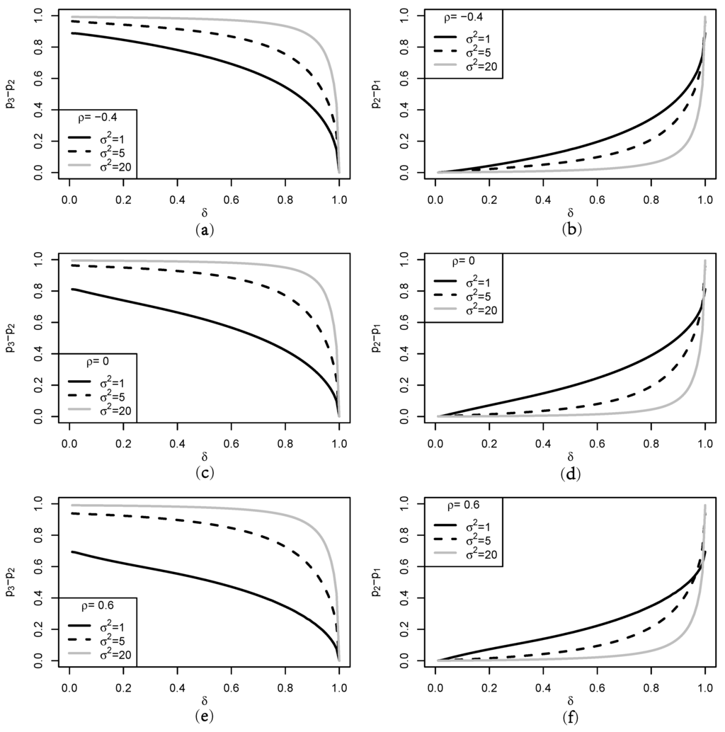
Figure 1. Graphs of the difference between $p_1={\gamma }_{max},$ $p_2={\gamma }_{two}$ and $p_3={\gamma }_{const}$. (a), (c), and (e) for the difference between $p_3$ and $p_2$; (b), (d), and (f) for the difference between $p_2$ and $p_1$.

3.2. Properties of the Entropy

The expected uncertainty in the multivariate interval constraint of the location parameter $\mathit{\theta }$, $\left\{\mathit{\theta };\mathit{\theta }\in \mathbf{C}\right\},$ accounted for by the two-stage prior ${\pi }_{two}\left(\mathit{\theta }\right)$, is measured by its entropy $Ent\left({\pi }_{two}\left(\mathit{\theta }\right)\right)$, and information about the constraint is defined by $-Ent\left({\pi }_{two}\left(\mathit{\theta }\right)\right).$ Thus, as considered by [20,28], the difference between the Shannon measures of information, before and after applying the uncertain constraint $\{\mathit{\theta };\mathit{\theta }\in \mathbf{C}\},$ can be explained by the following property.

Corollary 5. 

When ${\mathit{\theta }}_0$ is the centroid of the multivariate interval $\mathbf{C},$

$$\begin{array}{c}\hfill Ent\left({\pi }_{max}\left(\mathit{\theta }\right)\right)\ge Ent\left({\pi }_{two}\left(\mathit{\theta }\right)\right)\ge Ent\left({\pi }_{const}\left(\mathit{\theta }\right)\right),\end{array}$$

(16)

where $Ent\left({\pi }_{two}\left(\mathit{\theta }\right)\right)$ reduces to $Ent\left({\pi }_{max}\left(\mathit{\theta }\right)\right)$ for ${\mathrm{\Omega }}_1=\mathbf{O},$ while $Ent\left({\pi }_{two}\left(\mathit{\theta }\right)\right)$ is equal to $Ent\left({\pi }_{const}\left(\mathit{\theta }\right)\right)$ for ${\mathrm{\Omega }}_2=\mathbf{O}.$ All of the equalities hold for $\mathbf{C}={\mathbb{R}}^p.$

Proof. It is straightforward to check the equalities by using the stochastic representation in Equation (12). Since ${\pi }_{max}\left(\mathit{\theta }\right)$ is the maximum entropy prior, it is sufficient to show that $Ent\left({\pi }_{two}\left(\mathit{\theta }\right)\right)\ge Ent\left({\pi }_{const}\left(\mathit{\theta }\right)\right).$ First, $\mathrm{\Sigma }-{\mathrm{\Omega }}_1={\mathrm{\Omega }}_2>0$ implies that ${\overline{\mathrm{\Phi }}}_p(\mathbf{C};{\mathit{\theta }}_0,{\mathrm{\Omega }}_1)\ge {\overline{\mathrm{\Phi }}}_p(\mathbf{C};{\mathit{\theta }}_0,\mathrm{\Sigma })$ by the lemma of [27]. Second, ${\gamma }_{const}=Pr\left({\mathbf{Y}}_1+{\mathbf{Y}}_2\in (\mathit{\alpha },\mathit{\beta })|{\mathbf{Y}}_1+{\mathbf{Y}}_2\in (\mathit{\alpha },\mathit{\beta })\right)\ge Pr\left({\mathbf{Y}}_1+{\mathbf{Y}}_2\in (\mathit{\alpha },\mathit{\beta })|{\mathbf{Y}}_1\in (\mathit{\alpha },\mathit{\beta })\right)={\gamma }_{two}$ by Corollary 4. This and the lemma of [27] indicate that $Cov\left({\mathbf{Y}}_1+{\mathbf{Y}}_2|{\mathbf{Y}}_1\in (\mathit{\alpha },\mathit{\beta })\right)-Cov\left({\mathbf{Y}}_1+{\mathbf{Y}}_2|{\mathbf{Y}}_1+{\mathbf{Y}}_2\in (\mathit{\alpha },\mathit{\beta })\right)$ is a positive-semi-definite, and hence, $\mathrm{tr}\left({\mathrm{\Sigma }}^{-1}{E}_{two}\left[(\mathit{\theta }-{\mathit{\theta }}_0){(\mathit{\theta }-{\mathit{\theta }}_0)}^{\top }\right]\right)\ge \mathrm{tr}\left({\mathrm{\Sigma }}^{-1}{E}_{const}\left[(\mathit{\theta }-{\mathit{\theta }}_0){(\mathit{\theta }-{\mathit{\theta }}_0)}^{\top }\right]\right)$ by ([29], p. 54), where $E_{two}\left[(\mathit{\theta }-{\mathit{\theta }}_0){(\mathit{\theta }-{\mathit{\theta }}_0)}^{\top }\right]=Cov\left({\mathbf{Y}}_1+{\mathbf{Y}}_2|{\mathbf{Y}}_1\in (\mathit{\alpha },\mathit{\beta })\right)$ and $E_{const}\left[(\mathit{\theta }-{\mathit{\theta }}_0){(\mathit{\theta }-{\mathit{\theta }}_0)}^{\top }\right]=Cov\left({\mathbf{Y}}_1+{\mathbf{Y}}_2|{\mathbf{Y}}_1+{\mathbf{Y}}_2\in (\mathit{\alpha },\mathit{\beta })\right)$ for $\mathit{\alpha }=-\mathit{\beta }.$ These two results give the inequality $Ent\left({\pi }_{two}\left(\mathit{\theta }\right)\right)\ge Ent\left({\pi }_{const}\left(\mathit{\theta }\right)\right),$ because $E_{two}\left[logh\left(\mathit{\theta }\right)\right]\le 0.$

Figure 2 depicts the difference between $Ent\left({\pi }_{max}\left(\mathit{\theta }\right)\right),$ $Ent\left({\pi }_{two}\left(\mathit{\theta }\right)\right)$ and $Ent\left({\pi }_{const}\left(\mathit{\theta }\right)\right)$ using the same parameter values used in constructing Figure 1. Figure 2 coincides with the inequality relation given in Corollary 5 and indicates the following consequences: (i) Even though ${\mathit{\theta }}_0$ is not the centroid of the multivariate interval $\mathbf{C},$ we see that $Ent\left({\pi }_{max}\left(\mathit{\theta }\right)\right)>Ent\left({\pi }_{two}\left(\mathit{\theta }\right)\right)>Ent\left({\pi }_{const}\left(\mathit{\theta }\right)\right)$ for $\delta \in (0,1).$ (ii) The difference $Ent\left({\pi }_{two}\left(\mathit{\theta }\right)\right)-Ent\left({\pi }_{const}\left(\mathit{\theta }\right)\right)$ is a monotone decreasing function of $\delta ,$ while $Ent\left({\pi }_{max}\left(\mathit{\theta }\right)\right)-Ent\left({\pi }_{two}\left(\mathit{\theta }\right)\right)$ is a monotone increasing function. (iii) The differences get bigger the larger ${\sigma }^2$ becomes for $\delta \in (0,1).$ This indicates that the entropy of ${\pi }_{two}\left(\mathit{\theta }\right)$ is associated not only with the covariance of the first stage prior ${\mathrm{\Omega }}_2$, but that of the second stage prior ${\mathrm{\Omega }}_1$ in Equations (8) and (9), respectively. (iv) Upon comparing Figure 1 and Figure 2, the entropy $Ent\left({\pi }_{two}\left(\mathit{\theta }\right)\right)$ is closely related to the degree of belief ${\gamma }_{two}$, such that:

$$Ent\left({\pi }_{two}\left(\mathit{\theta }\right)\right)=c_{two}(1-{\gamma }_{two}),$$

where $c_{two}>0$ is obtained by using Equations (13) and (16) and $1-{\gamma }_{two}$ denotes the degree of uncertainty in a priori information regarding the multivariate interval constraint $\left\{\mathit{\theta };\mathit{\theta }\in \mathbf{C}\right\}$ elicited by ${\pi }_{two}\left(\mathit{\theta }\right).$ These consequences and Corollary 5 indicate that $1-{\gamma }_{two}$ stands between $1-{\gamma }_{const}$ and $1-{\gamma }_{max}.$ Thus, the two-stage prior ${\pi }_{two}\left(\mathit{\theta }\right)$ is useful for eliciting uncertain information about the multivariate interval constraint. Theorem 1 and the above statements produce an objective method for eliciting the stochastic constraint $\{\mathit{\theta };\mathit{\theta }\in \mathbf{C}\}$ via ${\pi }_{two}\left(\mathit{\theta }\right).$

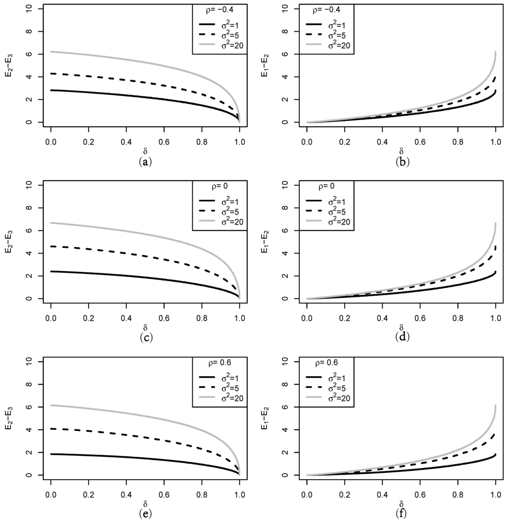
Figure 2. Graphs of the entropy difference between $E_1=Ent\left({\pi }_{max}\left(\mathit{\theta }\right)\right),$ $E_2=Ent\left({\pi }_{two}\left(\mathit{\theta }\right)\right)$ and $E_3=Ent\left({\pi }_{const}\left(\mathit{\theta }\right)\right)$ for different values of $\delta \in [0,1].$ (a), (c), and (e) for the difference between $E_2$ and $E_3$; (b), (d), and (f) for the difference between $E_1$ and $E_2$.

Corollary 6. 

Suppose the degree ($1-{\gamma }_{two}$) of uncertainty associated with the stochastic constraint $\{\mathit{\theta };\mathit{\theta }\in \mathbf{C}\}$ is given. An objective way of eliciting the prior information by using ${\pi }_{two}\left(\mathit{\theta }\right)$ is to choose the covariance matrices ${\mathrm{\Omega }}_1$ and ${\mathrm{\Omega }}_2$ in ${\pi }_{two}\left(\mathit{\theta }\right)$, such that ${\gamma }_{two}={\overline{\mathrm{\Phi }}}_{2p}\left({\mathbf{C}}^{*};\mathit{\tau },\mathrm{\Psi }\right)/{\overline{\mathrm{\Phi }}}_p\left(\mathbf{C};{\mathit{\theta }}_0,{\mathrm{\Omega }}_1\right),$ where $\mathrm{\Sigma }={\mathrm{\Omega }}_1+{\mathrm{\Omega }}_2$ is known and ${\mathrm{\Omega }}_1=\delta \mathrm{\Sigma }$ with $\delta \in [0,1].$

Since ${\gamma }_{const}=1$, the degree of uncertainty ( $1-{\gamma }_{two}$) is equal to ${\gamma }_{const}-{\gamma }_{two}.$ The left panel of Figure 1 plots a graph of $1-{\gamma }_{two}$ against $\delta .$ The graph indicates that a δ value for ${\pi }_{two}\left(\mathit{\theta }\right)$ can be easily determined for given $\mathrm{\Sigma },$ and the value is in inverse proportion to the degree of uncertainty regardless of $\mathrm{\Sigma }.$

3.3. Posterior Distribution

Suppose the distribution of the error vector in the model (1) belongs to the family of scale mixture of normal distributions defined in Equation (2); then, the conditional distribution of the data information from $n=1$ is $\left[\mathit{y}\right|\eta ]\sim N_p(\mathit{\theta },\kappa \left(\eta \right)\mathrm{\Lambda }).$ It is well known that the priors ${\pi }_{max}\left(\mathit{\theta }\right)$ and ${\pi }_{const}\left(\mathit{\theta }\right)$ are conjugate priors for the location vector $\mathit{\theta },$ provided that η and Λ are known. That is, conditional on $\eta ,$ each prior satisfies the conjugate property that the prior and the posterior distributions of $\mathit{\theta }$ belong to the same family of distributions. The following corollary provides that the conditional conjugate property also applies to ${\pi }_{two}\left(\mathit{\theta }\right).$

Corollary 7. 

Let $\left[\mathit{y}|\eta \right]\sim N_p(\mathit{\theta },\kappa \left(\eta \right)\mathrm{\Lambda })$ with known $\mathrm{\Lambda }.$ Then, the two-stage maximum entropy prior ${\pi }_{two}\left(\mathit{\theta }\right)$ in Equation (10) yields the conditional posterior distribution of $\mathit{\theta }$ given by:

$$\begin{array}{ccc}\hfill \left[\mathit{\theta }|\mathit{y},\eta \right]& \sim & RS{N}_p(\mathbf{C};{\mathit{\tau }}_{\eta }^{*},{\mathrm{\Psi }}_{\eta }^{*}),\hfill \end{array}$$

(17)

where ${\mathrm{\Omega }}_1=\delta \mathrm{\Sigma },$ $\delta \in (0,1),$ $\mathrm{\Sigma }={\mathrm{\Omega }}_1+{\mathrm{\Omega }}_2,$ ${\mathrm{\Sigma }}_{1\eta }^{*}=\delta (1-\delta )\mathrm{\Sigma }+{\delta }^2{\mathrm{\Sigma }}_{\eta }^{*},$ ${\mathrm{\Sigma }}_{\eta }^{*}={\left(\kappa {\left(\eta \right)}^{-1}{\mathrm{\Lambda }}^{-1}+{\mathrm{\Sigma }}^{-1}\right)}^{-1},$

$${\mathit{\tau }}_{\eta }^{*}=\left(\begin{array}{c}{\mathit{\theta }}_{0\eta }^{*}\\ {\mathit{\theta }}_{\eta }^{*}\end{array}\right),{\mathrm{\Psi }}_{\eta }^{*}=\left(\begin{array}{cc}{\mathrm{\Sigma }}_{1\eta }^{*}& \delta {\mathrm{\Sigma }}_{\eta }^{*}\\ \delta {\mathrm{\Sigma }}_{\eta }^{*}& {\mathrm{\Sigma }}_{\eta }^{*}\end{array}\right),{\mathit{\theta }}_{0\eta }^{*}=(1-\delta ){\mathit{\theta }}_0+\delta {\mathit{\theta }}_{\eta }^{*},and{\mathit{\theta }}_{\eta }^{*}={\mathrm{\Sigma }}_{\eta }^{*}\left(\kappa {\left(\eta \right)}^{-1}{\mathrm{\Lambda }}^{-1}\mathit{y}+{\mathrm{\Sigma }}^{-1}{\mathit{\theta }}_0\right).$$

Proof. 

When the two-stage prior ${\pi }_{two}\left(\mathit{\theta }\right)$ in Equation (10) is used, the conditional posterior density of $\mathit{\theta }$ given η is:

$$\begin{array}{ccc}\hfill p\left(\mathit{\theta }\right|\mathit{y},\eta )& \propto & {\varphi }_p(\mathit{y};\mathit{\theta },\kappa \left(\eta \right)\mathrm{\Lambda }){\varphi }_p(\mathit{\theta };{\mathit{\theta }}_0,\mathrm{\Sigma }){\overline{\mathrm{\Phi }}}_p\left(\mathbf{C};\mathit{\mu },Q\right)/{\overline{\mathrm{\Phi }}}_p\left(\mathbf{C};{\mathit{\theta }}_0,{\mathrm{\Omega }}_1\right),\hfill \\ & \propto & {\varphi }_p(\theta ;{\mathit{\theta }}_{\eta }^{*},{\mathrm{\Sigma }}_{\eta }^{*}){\overline{\mathrm{\Phi }}}_p\left(\mathbf{C};{\mathit{\mu }}_{\eta }^{*},Q_{\eta }^{*}\right),\hfill \end{array}$$

in that ${\overline{\mathrm{\Phi }}}_p\left(\mathbf{C};\mathit{\mu },Q\right)={\overline{\mathrm{\Phi }}}_p\left(\mathbf{C};{\mathit{\mu }}_{\eta }^{*},Q_{\eta }^{*}\right),$ where $\mathit{\mu }={\mathit{\theta }}_0+{\mathrm{\Omega }}_1{\mathrm{\Sigma }}^{-1}(\mathit{\theta }-{\mathit{\theta }}_0),$ ${\mathit{\mu }}_{\eta }^{*}={\mathit{\theta }}_{0\eta }^{*}+\delta (\mathit{\theta }-{\mathit{\theta }}_{\eta }^{*})$ and $Q_{\eta }^{*}={\mathrm{\Sigma }}_{1\eta }^{*}-{\delta }^2{\mathrm{\Sigma }}_{\eta }^{*}.$ The last term of the proportional relations is a kernel of the $RS{N}_p(\mathbf{C};{\mathit{\tau }}_{\eta }^{*},{\psi }_{\eta }^{*})$ density defined by Corollary 3. ☐

Corollaries 3 and 7 establish the conditional conjugate property of ${\pi }_{two}\left(\mathit{\theta }\right):$ Suppose the location parameter $\mathit{\theta }$ is the normal mean vector, then the $RSN$ prior distribution, i.e., ${\pi }_{two}\left(\mathit{\theta }\right),$ yields the conditional posterior distribution, which belongs to the class of $RSN$ distributions as given in Corollary 7. In the particular case where the distribution of η degenerates at $\kappa \left(\eta \right)=1,$ i.e., the model (1) is a normal model, then the conditional conjugate property of ${\pi }_{two}\left(\mathit{\theta }\right)$ reduces to the unconditional conjugate property.

Using the relation between the distribution of Equation (11) and that of Equation (12), we can obtain the stochastic representation for the conditional posterior $RSN$ distribution in Equation (17) as follows.

Corollary 8. 

Conditional on the mixing variable η, the stochastic representation of $\left[\mathit{\theta }|\mathit{y},\eta \right]\sim RS{N}_p(\mathbf{C};{\mathit{\tau }}_{\eta }^{*},{\mathrm{\Psi }}_{\eta }^{*})$ is:

$$\begin{array}{ccc}\hfill \left[\mathit{\theta }\right|\mathit{y},\eta ]& \stackrel{d}{=}& {\mathit{\theta }}_{\eta }^{*}+\delta {\mathrm{\Sigma }}_{\eta }^{*}{\mathrm{\Sigma }}_{1\eta }^{*-1}{\mathbf{W}}_1^{({\mathit{\alpha }}_{\eta }^{*},{\mathit{\beta }}_{\eta }^{*})}+{\left({\mathrm{\Sigma }}_{\eta }^{*}-{\delta }^2{\mathrm{\Sigma }}_{\eta }^{*}{\mathrm{\Sigma }}_{1\eta }^{*-1}{\mathrm{\Sigma }}_{\eta }^{*}\right)}^{1/2}{\mathbf{W}}_2,\hfill \end{array}$$

(18)

where ${\mathbf{W}}_1\sim N_p(\mathbf{0},{\mathrm{\Sigma }}_{1\eta }^{*})$ and ${\mathbf{W}}_2\sim N_p(\mathbf{0},I_p)$ are independent and ${\mathbf{W}}_1^{({\mathit{\alpha }}_{\eta }^{*},{\mathit{\beta }}_{\eta }^{*})}\stackrel{d}{=}\left[{\mathbf{W}}_1|{\mathbf{W}}_1\in ({\mathit{\alpha }}_{\eta }^{*},{\mathit{\beta }}_{\eta }^{*})\right],$ where ${\mathit{\alpha }}^{*}=\mathbf{a}-{\mathit{\theta }}_{0\eta }^{*}$ and ${\mathit{\beta }}^{*}=\mathbf{b}-{\mathit{\theta }}_{0\eta }^{*}.$

Proof. 

Suppose the distributions of ${\mathbf{X}}_1$ and ${\mathbf{X}}_2$ in Equation (11) changed to ${\mathbf{X}}_1\stackrel{d}{=}{\mathit{\theta }}_{0\eta }^{*}+{\mathbf{W}}_1$ and ${\mathbf{X}}_{\mathbf{2}}\stackrel{d}{=}{\mathit{\theta }}_{\eta }^{*}+\delta {\mathrm{\Sigma }}_{\eta }^{*}{\mathrm{\Sigma }}_{1\eta }^{*-1}{\mathbf{W}}_1+{\left({\mathrm{\Sigma }}_{\eta }^{*}-{\delta }^2{\mathrm{\Sigma }}_{\eta }^{*}{\mathrm{\Sigma }}_{1\eta }^{*-1}{\mathrm{\Sigma }}_{\eta }^{*}\right)}^{1/2}{\mathbf{W}}_2.$ Then, the stochastic representation in Equation (12) associated with the distribution $\left[{\mathbf{X}}_2|{\mathbf{X}}_1\in \mathbf{C}\right]$ in Equation (11) gives the result. ☐

4. Hierarchical Constrained Scale Mixture of Normal Model

For the model (1), if we are completely sure about a multivariate interval constraint on $\mathit{\theta },$ a suitable restriction on the parameter space $\theta \in {\mathbb{R}}^p,$ such as using a truncated normal prior distribution, is expected for eliciting the information. However, there are certain cases where we have a priori information that the location parameter $\mathit{\theta }$ is highly likely to have a multivariate interval constraint, and thus, the value of $\mathit{\theta }$ needs to be located with uncertainty in a restricted space $\{\mathit{\theta }\in \mathbf{C}\}$ with $\mathbf{C}=(\mathbf{a},\mathbf{b})$. Then, we cannot be sure about the constraint, and then, the constraint becomes stochastic (or uncertain), as in our problem of interest. In this case, the uncertainty about the constraint must be taken into account in the estimation procedure of the model (1). This section considers a hierarchical Bayesian estimation of the scale mixture of normal models reflecting the uncertain prior belief on $\mathit{\theta }.$

4.1. The Hierarchical Model

Let us consider a hierarchical constrained scale mixture of normal model (HCSMN) that uses the hierarchy of the scale mixture of normal model (1) and includes the two stages of a prior hierarchy in the following way:

$$\begin{array}{ccc}\hfill \left[{\mathit{y}}_i|{\eta }_i,\mathrm{\Lambda }\right]& =& \mathit{\theta }+{\mathit{ϵ}}_i,{\mathit{ϵ}}_i\sim N_p(0,\kappa \left({\eta }_i\right)\mathrm{\Lambda }),i=1,\dots ,n,\hfill \\ \hfill \mathit{\theta }|{\mathit{\mu }}_0& \sim & N_p({\mathit{\mu }}_0,{\mathrm{\Omega }}_2),\text{independent of }{({\mathit{ϵ}}_1,\cdots ,{\mathit{ϵ}}_n)}^{\top },\hfill \\ \hfill {\mathit{\mu }}_0& \sim & N_p({\mathit{\theta }}_0,{\mathrm{\Omega }}_1)\mathrm{I}({\mathit{\mu }}_0\in \mathbf{C}),\hfill \\ \hfill \mathrm{\Lambda }& \sim & W_p^{-1}(D,d),d>2p,\hfill \\ \hfill {\eta }_i& \stackrel{iid}{\sim }& g\left(\eta \right),i=1,\dots ,n,\hfill \end{array}$$

(19)

where $W_p^{-1}(D,d)$ denotes the inverted Wishart distribution with positive definite scale matrix D and d degrees of freedom whose pdf $W_p^{-1}(\mathrm{\Lambda };D,d)$ is:

$$W_p^{-1}(\mathrm{\Lambda };D,d)\propto {\left|\mathrm{\Lambda }\right|}^{-d/2}exp\left\{-\frac{1}{2}\mathrm{tr}\left({\mathrm{\Lambda }}^{-1}D\right)\right\},$$

${\mathrm{\Omega }}_1+{\mathrm{\Omega }}_2=\mathrm{\Sigma }$ with ${\mathrm{\Omega }}_1=\delta \mathrm{\Sigma },$ and $\delta \in [0,1].$

4.2. The Gibbs Sampler

Based on the HCSMN model structure with the likelihood and the prior distributions in Equation (19), the joint posterior distribution of $\mathit{\theta },$ Λ and $\mathit{\eta }={({\eta }_1,\dots ,{\eta }_n)}^{\top }$ given the data $\{{\mathit{y}}_1,\dots ,{\mathit{y}}_n\}$ is:

$$\begin{array}{ccc}\hfill p(\mathit{\theta },\mathrm{\Lambda },\mathit{\eta }|Data)& \propto & \prod _{i=1}^n{\left|\kappa \left({\eta }_i\right)\mathrm{\Lambda }\right|}^{-1/2}exp\left\{-\frac{1}{2}\mathrm{tr}\left[{\mathrm{\Lambda }}^{-1}\kappa {\left({\eta }_i\right)}^{-1}({\mathit{y}}_i-\mathit{\theta }){({\mathit{y}}_i-\mathit{\theta })}^{\top }\right]\right\}\hfill \\ & \times & {\varphi }_p(\mathit{\theta };{\mathit{\mu }}_0,{\mathrm{\Omega }}_2){\varphi }_p({\mathit{\mu }}_0;{\mathit{\theta }}_0,{\mathrm{\Omega }}_1)I({\mathit{\mu }}_0\in \mathbf{C})\hfill \\ & \times & {\left|\mathrm{\Lambda }\right|}^{-d/2}exp\left\{-\frac{1}{2}\mathrm{tr}\left({\mathrm{\Lambda }}^{-1}D\right)\right\}\prod _{i=1}^n{g}_i\left({\eta }_i\right),\hfill \end{array}$$

(20)

where $g\left({\eta }_i\right)$’s denote the densities of the mixing variables ${\eta }_i$’s. Note that the joint posterior of Equation (20) is not simplified in an analytic form of the known density and, thus, intractable for the posterior inference. Instead, we use the Gibbs sampler for the posterior inference. See [30] for a reference. To run the Gibbs sampler, we need the following full conditional posterior distributions:

(i)

The full conditional posterior densities of ${\eta }_i$’s are given by:

$$\begin{array}{ccc}\hfill p\left({\eta }_i\right|\mathit{\theta },\mathrm{\Lambda },{\mathit{y}}_i)& \propto & \kappa {\left({\eta }_i\right)}^{-\frac{p}{2}}exp\left\{-\frac{{({\mathit{y}}_i-\mathit{\theta })}^{\top }{\mathrm{\Lambda }}^{-1}({\mathit{y}}_i-\mathit{\theta })}{2\kappa \left({\eta }_i\right)}\right\}g\left({\eta }_i\right),i=1,\dots ,n,\hfill \end{array}$$

(21)

(ii)

The full conditional distribution of $\mathit{\theta }$ is obtained by using the way analogous to the proof of Corollary 7. It is:

$$\left[\mathit{\theta }|\mathrm{\Lambda },\mathit{\eta },Data\right]\sim RS{N}_p\left(\mathbf{C};{\mathit{\tau }}_{pos},{\mathrm{\Psi }}_{pos}\right),$$

(22)

where:

$${\mathit{\tau }}_{pos}=\left(\begin{array}{c}{\mathit{\tau }}_0\\ {\mathit{\tau }}_1\end{array}\right),{\mathrm{\Psi }}_{pos}\left(\begin{array}{cc}{\mathrm{\Omega }}_0^{*}& \delta {\mathrm{\Omega }}^{*}\\ \delta {\mathrm{\Omega }}^{*}& {\mathrm{\Omega }}^{*}\end{array}\right),{\mathit{\tau }}_0=(1-\delta ){\mathit{\theta }}_0+\delta {\mathit{\tau }}_1,$$

${\mathit{\tau }}_1={\mathrm{\Omega }}^{*}\left({\mathrm{\Sigma }}^{-1}{\mathit{\theta }}_0+{\sum }_{i=1}^n{\left(\kappa \left({\eta }_i\right)\mathrm{\Lambda }\right)}^{-1}{\mathit{y}}_i\right),$ ${\mathrm{\Omega }}^{*}={\left({\mathrm{\Sigma }}^{-1}+{\sum }_{i=1}^n{\left(\kappa \left({\eta }_i\right)\mathrm{\Lambda }\right)}^{-1}\right)}^{-1},$ and ${\mathrm{\Omega }}_0^{*}=\delta (1-\delta )\mathrm{\Sigma }+{\delta }^2{\mathrm{\Omega }}^{*}.$

(iii)

The full conditional posterior distribution of Λ is an inverse-Wishart distribution:

$$\left[\mathrm{\Lambda }|\mathit{\theta },\mathit{\eta },Data\right]\sim W_p^{-1}\left(V,m\right),m>2p,$$

(23)

where $V=D+{\sum }_{i=1}^n\kappa {\left({\eta }_i\right)}^{-1}({\mathit{y}}_i-\mathit{\theta }){({\mathit{y}}_i-\mathit{\theta })}^{\top }$ and $m=n+d.$

4.3. Markov Chain Monte Carlo Sampling Scheme

When conducting a posterior inference of the HCSMN model, using the Gibbs sampling algorithm with the full conditional posterior distributions of ${\eta }_i$’s, $\mathit{\theta }$ and Λ, the following points should be noted.

• note 1: Variable ${\eta }_i$ at $\kappa \left({\eta }_i\right)=1,$ i.e., the HCN (hierarchical constrained normal) model with ${\mathit{ϵ}}_i\stackrel{iid}{\sim }{N}_p(\mathbf{0},\mathrm{\Lambda }),$ $i=1,\dots ,n,$ the Gibbs sampler consists of two conditional distributions $\left[\mathit{\theta }\right|\mathrm{\Lambda },Data]$ and $\left[\mathrm{\Lambda }\right|\mathit{\theta },Data].$ To sample from the first full conditional posterior distribution, we can utilize the stochastic representations of the $RSN$ distribution in Corollary 8. The R package tmvtnorm and the R package mvtnorm can be used to sample from the $RSN$ distribution in Equation (22).
• note 2: According to choice of the distribution ${\eta }_i$ and the mixing function $\kappa \left({\eta }_i\right),$ the HCSMN model may produce a different model other than the HCN model, such as hierarchical constrained multivariate $t_{\nu }$ (HC$t_{\nu }$), hierarchical constrained multivariate $logit$, hierarchical constrained multivariate $stable$ and hierarchical constrained multivariate $exponential$ $power$ models. See, e.g., [31,32], for various distributions of ${\eta }_i$ and corresponding function $\kappa \left({\eta }_i\right)$, which can be used to construct the HCSMN model.
• note 3: When the hierarchical constrained multivariate $t_{\nu }$ (HC$t_{\nu }$) model is considered, the hierarchy of the model in Equation (19) consists of ${\mathit{ϵ}}_i\stackrel{iid}{\sim }{N}_p(\mathbf{0},\kappa \left({\eta }_i\right)\mathrm{\Lambda })$ with $\kappa \left({\eta }_i\right)={\eta }_i^{-1}$ and ${\eta }_i\sim Gamma(\nu /2,\nu /2),$ $i=1,\dots ,n.$ Thus, the Gibbs sampler comprises the conditional posterior Equations (21)–(23). Under the HC$t_{\nu }$ model, the distribution of Equation (21) reduces to:

  $$\left[{\eta }_i\right|\mathit{\theta },\mathrm{\Lambda },{\mathit{y}}_i]\sim Gamma({\nu }^{*}/2,h/2),$$

  where ${\nu }^{*}=p+\nu$ and $h=\nu +{({\mathit{y}}_i-\mathit{\theta })}^{\top }{\mathrm{\Lambda }}^{-1}({\mathit{y}}_i-\mathit{\theta }).$ To limit model complexity, we consider only fixed ν, so that we can investigate different HC$t_{\nu }$ models. As suggested by [32], a uniform prior on $1/\nu$ ($0<1/\nu <1$) can be considered. However, this will bring additional computational burden.
• note 4: Except for the HCN and HC$t_{\nu }$ models, the Metropolis–Hastings algorithm within the Gibbs sampler is used for estimating the HCSMN models, because the conditional posterior densities Equation (20) do not have explicit forms of known distributions as in Equations (21) and (22). See, e.g., [22], for the algorithm for sampling ${\eta }_i$ from various mixing distributions, $g_i\left({\eta }_i\right).$ A general procedure for the algorithm is as follows: Given the current values $\mathrm{\Theta }=\{\mathit{\eta },\mathit{\theta },\mathrm{\Lambda }\}$, we independently generate a candidate ${\eta }_i$ from a proposal density $q\left({\eta }_i^{*}\right|{\eta }_i)=g_i\left({\eta }_i^{*}\right),$ as suggested by [33], which is used for a Metropolis–Hastings algorithm. Then, accept the candidate value with the acceptance rate:

  $$\alpha ({\eta }_i,{\eta }_i^{*})=min\left\{\frac{p\left(\mathrm{\Theta }\right|{\eta }_i^{*})}{p\left(\mathrm{\Theta }\right|{\eta }_i)},1\right\}$$

  $i=1,\dots ,n.$ Because the target density is proportional to $p\left(\mathrm{\Theta }\right|{\eta }_i)g_i\left({\eta }_i\right)$ and $p\left(\mathrm{\Theta }\right|{\eta }_i)={\varphi }_p({\mathit{y}}_i;\mathit{\theta },\kappa \left({\eta }_i\right)\mathrm{\Lambda })$ is uniformly bounded for ${\eta }_i>0.$
• note 5: As noted from Equations (8) and (9), the second and third stage priors of the HCSMN model in Equation (19) reduce to the two-stage prior ${\pi }_{two}\left(\mathit{\theta }\right),$ eliciting the stochastic multivariate interval constraint with degree of uncertainty $1-{\gamma }_{two}.$ Instead, if the maximum entropy prior ${\pi }_{max}\left(\mathit{\theta }\right)$ and the constrained maximum entropy prior ${\pi }_{const}\left(\mathit{\theta }\right)$ are used for the HCSMN, then the respective full conditional distributions of $\mathit{\theta }$ of the Gibbs sampler change from Equation (22) to:

  $$\left[\mathit{\theta }|\mathrm{\Lambda },\mathit{\eta },Data\right]\sim N_p\left({\mathit{\tau }}_1,{\mathrm{\Omega }}^{*}\right)\mathrm{for}\mathit{\theta }\in {\mathbb{R}}^p\mathrm{and}\left[\mathit{\theta }|\mathrm{\Lambda },\mathit{\eta },Data\right]\sim N_p\left({\mathit{\tau }}_1,{\mathrm{\Omega }}^{*}\right)\mathrm{I}\left(\mathit{\theta }\in \mathbf{C}\right),$$

  where ${\mathit{\tau }}_1$ and ${\mathrm{\Omega }}^{*}$ are the same as given in Equation (22).

4.4. Bayes Estimation

For a simple example, let us consider the HCN model with known $\mathrm{\Lambda }.$ When we assume a stochastic constraint $\{\mathit{\theta };\mathit{\theta }\in \mathbf{C}\}$ obtained from a priori information, we may use the two-stage maximum entropy prior ${\pi }_{two}\left(\mathit{\theta }\right)$ defined by the second and third stages of the HCSMN model (19) with $\delta \in (0,1),$ where the value of δ is determined by using Corollary 6. This yields a Bayes estimate based on the two-stage maximum entropy prior. Corollary 8 yields:

$$\begin{array}{ccc}\hfill {\widehat{\mathit{\theta }}}_{two}& =& {\mathit{\tau }}_1+\delta {\mathrm{\Omega }}^{*}{\mathrm{\Omega }}_0^{*-1}E\left[{\mathit{\theta }}_{tn}^{*}\right]={\mathit{\tau }}_1+\delta {\mathrm{\Omega }}^{*}{\mathrm{\Omega }}_0^{*-1}\mathit{\zeta }\hfill \end{array}$$

(24)

and:

$$\mathit{\zeta }={({\zeta }_1,\dots ,{\zeta }_p)}^{\top }\mathrm{with}{\zeta }_i=w_{0i}\frac{\varphi (u_i/w_{0i})-\varphi (v_i/w_{0i})}{\mathrm{\Phi }(v_i/w_{0i})-\mathrm{\Phi }(u_i/w_{0i})},i=1,\dots ,p,$$

where ${\mathit{\theta }}_{tn}^{*}\sim N_p(\mathbf{0},{\mathrm{\Omega }}_0^{*})$I$\left({\mathit{\theta }}_{tn}^{*}\in (\mathbf{u},\mathbf{v})\right),$ a truncated normal distribution with $\mathbf{u}=\mathbf{a}-{\mathit{\tau }}_0={(u_1,\dots ,u_p)}^{\top }$ and $\mathbf{v}=\mathbf{b}-{\mathit{\tau }}_0={(v_1,\dots ,v_p)}^{\top }$ and $w_{0i}$ denotes i-th diagonal element of ${\mathrm{\Omega }}_0^{*}.$ Here, ${\mathit{\tau }}_1$ and ${\mathit{\tau }}_0$ are the same as those in Equation (22), and $\varphi (·)$ denotes the univariate standard normal density function. See [25,34] for the first moment of the truncated multivariate normal distribution and for a numerical calculation of the posterior covariance matrix $Cov\left({\mathit{\theta }}_{tn}^{*}\right),$ respectively.

On the other hand, when we have certainty about the constraint $\{\mathit{\theta };\mathit{\theta }\in \mathbf{C}\},$ we may use the HCSMN model with $\delta =1,$ which uses the constrained maximum entropy prior ${\pi }_{const}\left(\mathit{\theta }\right)$ instead of ${\pi }_{two}\left(\mathit{\theta }\right)$ in its hierarchy. This case gives the Bayes estimate:

$$\begin{array}{ccc}\hfill {\widehat{\mathit{\theta }}}_{const}& =& E\left[{\mathit{\theta }}_{tn}\right]={\mathit{\tau }}_1+{\mathit{\zeta }}^{*}\hfill \end{array}$$

(25)

and:

$${\mathit{\zeta }}^{*}={({\zeta }_1^{*},\dots ,{\zeta }_p^{*})}^{\top }\mathrm{with}{\zeta }_i^{*}=w_i\frac{\varphi (a_i/w_i)-\varphi (b_i/w_i)}{\mathrm{\Phi }(b_i/w_i)-\mathrm{\Phi }(a_i/w_i)},i=1,\dots ,p,$$

where ${\mathit{\theta }}_{tn}\sim N_p({\mathit{\tau }}_1,{\mathrm{\Omega }}^{*})$I$\left({\mathit{\theta }}_{tn}\in \mathbf{C}\right)$ and $w_i$ denotes i-th diagonal element of ${\mathrm{\Omega }}^{*}.$

On the contrary, when we have completely no a priori information about the constraint in the space of $\mathit{\theta },$ the HCSMN model with the maximum entropy prior ${\pi }_{max}\left(\mathit{\theta }\right)$ (equivalently, the HCSMN model with $\delta =0$) may be used for the posterior inference. In this model, the Bayes estimate of the location parameter is given by:

$$\begin{array}{ccc}\hfill {\widehat{\mathit{\theta }}}_{max}& =& {\mathit{\tau }}_1.\hfill \end{array}$$

(26)

Comparing Equations (24) and (25) to Equation (26), we see that Equations (24) and (25) are the same for $\delta =1$, and the last term in Equation (24) vanishes when we assume that there is no a priori information about the stochastic constraint, $\{\mathit{\theta };\mathit{\theta }\in \mathbf{C}\}.$ In this sense, the last term in Equation (24) can be interpreted as a shrinkage effect of the HCSMN model with $\delta \ne 0.$ This effect makes the Bayes estimator of $\mathit{\theta }$ shrink toward the stochastic constraint. In addition, we can calculate the difference between the estimates in Equations (24) and (25):

$$Diff={\widehat{\mathit{\theta }}}_{const}-{\widehat{\mathit{\theta }}}_{two}={\mathit{\zeta }}^{*}-\delta {\mathrm{\Omega }}^{*}{\mathrm{\Omega }}_0^{*-1}\mathit{\zeta }.$$

This difference vector is a function of the degree of belief ${\gamma }_{two}$ or $\delta \in (0,1)$ for Equation (25) is based on ${\gamma }_{const}=1$ and $\delta =1$ and $Diff=\mathbf{0}$ for $\delta =1.$ Thus, the difference represents a stochastic effect of the multivariate interval constraint.

5. Numerical Illustrations

This section presents an empirical analysis of the proposed approach (using the HCSMN model) to the stochastic multivariate interval constraint on the location model. We provide numerical simulation results and a real data application comparing the proposed approach to the hierarchical Bayesian approaches, which use usual priors, ${\pi }_{max}\left(\mathit{\theta }\right)$ and ${\pi }_{const}\left(\mathit{\theta }\right).$ For numerical implementations, we develop our program written in R, which is available from the author upon request.

5.1. Simulation Study

To examine the performance of the HSCMN model for estimating the location parameter with a stochastic multivariate interval constraint, we conduct a simulation study. The study is based up 200 synthetic datasets for different sample sizes $n=20,200$ generated form each distribution of $N_4(\mathit{\theta },\mathrm{\Lambda })$ and $t_4(\mathit{\theta },\mathrm{\Lambda },\nu ),$ a four-dimensional t with the location parameter $\mathit{\theta },$ scale matrix Λ and degrees of freedom $\nu =5.$ For the simulation, we used the following choice of parameter values: $\mathit{\theta }={(\theta ,\theta ,m\theta ,m\theta )}^{\top }$ and $\mathrm{\Lambda }=(1-\rho )I_4+\rho {\mathbf{1}}_4{\mathbf{1}}_4^{\top },$ where $m={(-1)}^{\theta +1},$ $\rho =0.5,$ and $\theta =1,2.$

To fit each of the 200 synthetic datasets (Dataset I) generated from the $N_4(\mathit{\theta },\mathrm{\Lambda })$ distribution, we implemented the Markov chain Monte Carlo (MCMC) posterior simulation with the three different HCN models with the multivariate interval constraint $\mathbf{C}={(\mathbf{a},\mathbf{b})}^{\top }$: the HCN models that use ${\pi }_{two}\left(\mathit{\theta }\right),$ ${\pi }_{max}\left(\mathit{\theta }\right),$ and ${\pi }_{const}\left(\mathit{\theta }\right).$ We denote these models by HCN$\left({\pi }_{two}\right)$, HCN$\left({\pi }_{max}\right)$ and HCN$\left({\pi }_{const}\right).$ For each dataset, MCMC posterior sampling was based on the first 10,000 posterior samples as the burn-in, followed by a further 100,000 posterior samples with a thinning size of 10. Thus, the final MCMC posterior samples with a size of 10,000 were obtained for each of the three HCN models. Exactly the same MCMC posterior sampling scheme is applied to each of the 200 synthetic datasets (Dataset II) from the $t_4(\mathit{\theta },\mathrm{\Lambda },\nu )$ distribution based on the three HC$t_{\nu }$ models, HC$t_{\nu }\left({\pi }_{two}\right)$, HC$t_{\nu }\left({\pi }_{max}\right)$ and HC$t_{\nu }\left({\pi }_{const}\right).$ To satisfy a subjective perspective of the hierarchical models, we set ${\mathit{\theta }}_0=\mathbf{0},$ $\mathrm{\Sigma }={\mathrm{\Omega }}_1+{\mathrm{\Omega }}_2=0.5\theta I_4,$ and ${\mathrm{\Omega }}_1=0.85\mathrm{\Sigma }$ to specify our information about the parameter $\mathit{\theta },$ while we set $D={10}^{-2}{I}_4$ and $d=2p+5$ to elicit no information about Λ (see, e.g., [32]). For the stochastic multivariate interval constraint, we set $\mathbf{a}=-0.5\theta {\mathbf{1}}_4$ and $\mathbf{b}=0.5\theta {\mathbf{1}}_4,$ and this constraint gives the degree of belief ${\gamma }_{max}=0.073$ (or $0.217$) and ${\gamma }_{two}=0.394$ (or $0.571$) for $\theta =1$ (or 2). Note that the degree of belief in the constraint, accounted for by ${\pi }_{const}\left(\mathit{\theta }\right),$ is ${\gamma }_{const}=1$ for all of the values of $\theta .$

Summary statistics of the posterior samples of the location parameters (the mean and the standard deviation of 200 posterior means of each parameter) along with the degrees of belief about the constraint $\mathbf{C}$ (${\gamma }_{max},$ ${\gamma }_{two}$ and ${\gamma }_{const}$) are listed in Table 1. For the sake of saving a space, we omit the summary statistics regarding Λ from the table. The table indicates the followings: (i) The MCMC method performs well in estimating the location parameters of all of the models considered. This can be justified by the estimation results of the HCN$\left({\pi }_{max}\right)$ and HC$t_{\nu }\left({\pi }_{max}\right)$ models. Specifically, in the posterior estimation of $\mathit{\theta },$ the data information tends to dominate the prior information about $\mathit{\theta }$ for the large sample case (i.e., $n=200$), while the latter tends to dominate the former for the small sample case of $n=20.$ Furthermore, the convergence of the MCMC sampling algorithm was evident, and a discussion about the convergence will be given in Subsection 5.2; (ii) The estimates of $\mathit{\theta }$ obtained from the HCN$\left({\pi }_{two}\right)$ and HC$t_{\nu }\left({\pi }_{two}\right)$ models are uniformly closer to the stochastic constraint $\mathit{\theta }\in \mathbf{C}$ than those from the HCN$\left({\pi }_{max}\right)$ and HC$t_{\nu }\left({\pi }_{max}\right)$ models. This confirms that ${\pi }_{two}\left(\mathit{\theta }\right)$ induces an obvious shrinkage effect in Bayesian estimation of the location parameter with a stochastic multivariate interval constraint; (iii) Comparing the estimates of $\mathit{\theta }$ obtained from the HCN$\left({\pi }_{two}\right)$ (or HC$t_{\nu }\left({\pi }_{two}\right))$ model to those from the HCN$\left({\pi }_{const}\right)$ (or HC$t_{\nu }\left({\pi }_{const}\right))$ model, we see that the difference between their vector values is significant. Thus, we can expect an apparent stochastic effect if we use ${\pi }_{two}\left(\mathit{\theta }\right)$ in Bayesian estimation of the location parameter with a stochastic multivariate interval constraint.

Table 1. Summaries of posterior samples of $\mathit{\theta }={({\theta }_1,{\theta }_2,{\theta }_3,{\theta }_4)}^{\top }$ obtained by using three different priors; ${\pi }_{two}\left(\mathit{\theta }\right),$ ${\pi }_{max}\left(\mathit{\theta }\right)$ and ${\pi }_{const}\left(\mathit{\theta }\right).$ HCN, hierarchical constrained normal.

	$\underset{\mathbf{\_}}{\mathbf{HCN}\mathbf{\left(}{\mathit{\pi }}_{\mathit{m}\mathit{a}\mathit{x}}\mathbf{\right)}}$				$\underset{\mathbf{\_}}{\mathbf{HCN}\left({\mathit{\pi }}_{\mathit{t}\mathit{w}\mathit{o}}\right)}$				$\underset{\mathbf{\_}}{\mathbf{HCN}\left({\mathit{\pi }}_{\mathit{c}\mathit{o}\mathit{n}\mathit{s}\mathit{t}}\right)}$
Dataset I	$\mathbf{(}{\mathit{\theta }}_{\mathbf{1}}$	${\mathit{\theta }}_{\mathbf{2}}$	${\mathit{\theta }}_{\mathbf{3}}$	${\mathit{\theta }}_{\mathbf{4}}\mathbf{)}$	$\mathbf{(}{\mathit{\theta }}_{\mathbf{1}}$	${\mathit{\theta }}_{\mathbf{2}}$	${\mathit{\theta }}_{\mathbf{3}}$	${\mathit{\theta }}_{\mathbf{4}}\mathbf{)}$	$\mathbf{(}{\mathit{\theta }}_{\mathbf{1}}$	${\mathit{\theta }}_{\mathbf{2}}$	${\mathit{\theta }}_{\mathbf{3}}$	${\mathit{\theta }}_{\mathbf{4}}\mathbf{)}$
$\underset{\_}{n=20}$
true	1.000	1.000	1.000	1.000	1.000	1.000	1.000	1.000	1.000	1.000	1.000	1.000
mean	0.853	0.862	0.869	0.857	0.525	0.530	0.542	0.549	0.141	0.112	0.139	0.121
s.d.	0.203	0.212	0.196	0.194	0.189	0.187	0.176	0.167	0.099	0.111	0.096	0.055
$\underset{\_}{n=200}$
true	1.000	1.000	1.000	1.000	1.000	1.000	1.000	1.000	1.000	1.000	1.000	1.000
mean	0.978	0.979	0.981	0.977	0.912	0.914	0.916	0.912	0.342	0.291	0.294	0.299
s.d.	0.073	0.072	0.074	0.068	0.060	0.067	0.069	0.064	0.037	0.058	0.077	0.064
$\underset{\_}{n=20}$
true	2.000	2.000	−2.000	−2.000	2.000	2.000	−2.000	−2.000	2.000	2.000	−2.000	−2.000
mean	1.837	1.846	−1.853	−1.842	1.306	1.314	−1.331	−1.349	0.599	0.501	−0.483	−0.493
s.d.	0.215	0.223	0.208	0.205	0.295	0.271	0.262	0.238	0.232	0.263	0.291	0.141
$\underset{\_}{n=200}$
true	2.000	2.000	−2.000	−2.000	2.000	2.000	−2.000	−2.000	2.000	2.000	−2.000	−2.000
mean	1.977	1.979	−1.980	−1.977	1.782	1.784	−1.785	−1.782	0.884	0.856	−0.795	−0.733
s.d.	0.074	0.072	0.074	0.068	0.068	0.065	0.068	0.062	0.029	0.051	0.068	0.062
	$\underset{\_}{\mathrm{HC}{t}_5\left({\pi }_{two}\right)}$				$\underset{\_}{\mathrm{HC}{t}_5\left({\pi }_{max}\right)}$				$\underset{\_}{\mathrm{HC}{t}_5\left({\pi }_{const}\right)}$
Dataset II	$({\theta }_1$	${\theta }_2$	${\theta }_3$	${\theta }_4)$	$({\theta }_1$	${\theta }_2$	${\theta }_3$	${\theta }_4)$	$({\theta }_1$	${\theta }_2$	${\theta }_3$	${\theta }_4)$
$\underset{\_}{n=20}$
true	1.000	1.000	1.000	1.000	1.000	1.000	1.000	1.000	1.000	1.000	1.000	1.000
mean	0.681	0.691	0.688	0.774	0.332	0.368	0.403	0.361	0.155	0.157	0.158	0.161
s.d.	0.172	0.182	0.201	0.205	0.198	0.190	0.218	0.186	0.108	0.112	0.120	0.099
$\underset{\_}{n=200}$
true	1.000	1.000	1.000	1.000	1.000	1.000	1.000	1.000	1.000	1.000	1.000	1.000
mean	1.003	0.974	1.033	1.006	0.802	0.818	0.814	0.806	0.362	0.411	0.341	0.351
s.d.	0.175	0.178	0.172	0.199	0.061	0.065	0.070	0.081	0.048	0.052	0.039	0.047
$\underset{\_}{n=20}$
true	2.000	2.000	−2.000	−2.000	2.000	2.000	−2.000	−2.000	2.000	2.000	−2.000	−2.000
mean	1.724	1.763	−1.764	−1.675	0.886	0.874	−0.857	−0.924	0.415	0.428	−0.496	−0.489
s.d.	0.239	0.230	0.245	0.231	0.324	0.319	0.343	0.313	0.201	0.196	0.193	0.204
$\underset{\_}{n=200}$
true	2.000	2.000	−2.000	−2.000	2.000	2.000	−2.000	−2.000	2.000	2.000	−2.000	−2.000
mean	2.018	1.943	−1.991	−2.103	1.702	1.699	−1.715	−1.689	0.967	0.986	−0.965	−0.959
s.d.	0.079	0.082	0.081	0.073	0.096	0.099	0.091	0.089	0.053	0.049	0.047	0.045

5.2. Car Body Assembly Data Example

John and Wichern consider car body assembly data (accessible through www.prenhall.com/statistics, [35]) obtained from a study of its sheet metal assembly process. A major automobile manufacturer uses sensors that record the deviation from the nominal thickness (millimeters $\times {10}^{-1}$) at a specific location on a car, which has the following levels: the deviation of the car body at the final stage of assembly ($Y_1$) and that at an early stage of assembly ($Y_2$). The data consist of 50 pairs of observations of ($Y_1$, $Y_2$), and they provide summary statistics as listed in Table 2. The tests given by ([36], p. 148), using the measures of multivariate skewness and kurtosis, accept the bivariate normality of the joint distribution of $Y={(Y_1,Y_2)}^{\top }.$ The respective skewness and kurtosis are $b_{1p}=0.074$ and $b_{2p}=7.337,$ which give respective p-values of 0.954 (chi-square test for the skewness) and 0.721 (normal test for the kurtosis), indicating the observation model for the dataset is:

$${\mathit{y}}_i=\mathit{\theta }+{\mathit{ϵ}}_i,i=1,\dots ,50,$$

where ${\mathit{ϵ}}_i\stackrel{iid}{\sim }{N}_2(\mathbf{0},\mathrm{\Lambda }),$ $\mathrm{\Lambda }=\left\{{\lambda }_{ij}\right\}.$ The Shapiro–Wilk (S-W) test is also implemented to see the marginal normality of each $Y_i,$ $i=1,2.$ The test statistic values and corresponding p-values of the S-W test are listed in Table 2.

Table 2. Summary statistics for the car body assembly data. S-W, Shapiro–Wilk.

Variable	Mean	s.d.	S-W	p-Value
$Y_1$	−1.996	2.781	0.959	0.083
$Y_2$	7.426	5.347	0.989	0.926

In practical situations, we may have information about the mean vector of the observation model (i.e., mean deviation from the nominal thickness) from a past study of the sheet metal assembly process or a quality control report of the automobile manufacturer. Suppose that the information about the centroid of the mean deviation vector, $\mathit{\theta }={({\theta }_1,{\theta }_2)}^{\top },$ is ${(-1,4)}^{\top }$ with $Cov\left(\mathit{\theta }\right)=diag\{1,4\}.$ Furthermore, there is uncertain information that $\mathit{\theta }\in (\mathbf{a},\mathbf{b}),$ where $\mathbf{a}={(-1.5,3)}^{\top }$ and $\mathbf{b}={(-0.5,5)}^{\top }.$ This paper has proposed the two-stage maximum entropy prior ${\pi }_{two}\left(\mathit{\theta }\right)$ to represent all of the information, which is not available with the other priors, such as ${\pi }_{max}\left(\mathit{\theta }\right)$ and ${\pi }_{const}\left(\mathit{\theta }\right)$.

Using the three hierarchical models (i.e., the HCN$\left({\pi }_{max}\right),$ HCN$\left({\pi }_{two}\right)$ and HCN$\left({\pi }_{const}\right)$ models), we obtain 10,000 posterior samples from the MCMC sampling scheme based on each of the three models with a 10 thinning period after a burn-in period of 10,000 samples. In estimating the Mote Carlo (MC) error, we used the batch mean method method with 50 batches; see, e.g., [37] (pp. 39–40). For a formal test for the convergence of the MCMC algorithm, we applied the Heidelberger–Welch diagnostic test of [38] to single-chain MCMC runs and calculated the p-values of the test. For the posterior simulation, we used the following choice of hyper-parameter values: ${\mathit{\theta }}_0={(-1,4)}^{\top },$ $\mathrm{\Sigma }={\mathrm{\Omega }}_1+{\mathrm{\Omega }}_2=10I_2,$ ${\mathrm{\Omega }}_1=\delta \mathrm{\Sigma },$ ${\mathrm{\Omega }}_2=(1-\delta )\mathrm{\Sigma },$ $\delta \in (0,1),$ $D={10}^{-2}{I}_2$ and $d={10}^2+2p+1.$ The posterior estimation and the convergence test results are shown in Table 3. Note that Columns 7–9 of the table list the values obtained from implementing the MCMC sampling for the posterior estimation of HCN(π_two).

Table 3. The posterior estimates and the convergence test results.

δ	${\mathit{\gamma }}_{\mathit{t}\mathit{w}\mathit{o}}$	Parameter	HCN$\mathbf{\left(}{\mathit{\pi }}_{\mathit{m}\mathit{a}\mathit{x}}\mathbf{\right)}$	HCN$\mathbf{\left(}{\mathit{\pi }}_{\mathit{c}\mathit{o}\mathit{n}\mathit{s}\mathit{t}}\mathbf{\right)}$	HCN$\mathbf{\left(}{\mathit{\pi }}_{\mathit{t}\mathit{w}\mathit{o}}\mathbf{\right)}$	s.d.	MC Error	p-Value
		${\theta }_1$	−1.874	−1.321	−1.665	0.581	0.005	0.483
		${\theta }_2$	7.045	4.814	6.332	1.089	0.008	0.354
0.8	0.423	${\lambda }_{11}$	7.549	7.863	7.682	1.231	0.007	0.551
		${\lambda }_{12}$	−4.632	−4.905	−4.819	1.631	0.005	0.671
		${\lambda }_{22}$	26.872	25.021	27.351	4.926	0.013	0.352
		${\theta }_1$	−1.874	−1.321	−1.557	0.496	0.004	0.434
		${\theta }_2$	7.045	4.814	5.905	1.112	0.006	0.298
0.9	0.567	${\lambda }_{11}$	7.526	7.781	7.959	1.317	0.008	0.635
		${\lambda }_{12}$	−4.726	−5.347	−4.989	1.546	0.006	0.712
		${\lambda }_{22}$	27.587	25.347	28.012	4.836	0.012	0.384

The small MC error values listed in Table 3 convince us of the convergence of the MCMC algorithm. Furthermore, the p-values of the Heidelberger–Welch test for the stationarity of the single MCMC run are larger than 0.1. Thus, both of the diagnostic checking methods advocate the convergence of the proposed MCMC sampling scheme. Similar to Table 1, this table also shows that ${\pi }_{two}\left(\mathit{\theta }\right)$ induces the shrinkage and stochastic effects in the Bayesian estimation of $\mathit{\theta }$ with the uncertain multivariate interval constraint: (i) From the comparison of the posterior estimates obtained from HCN$\left({\pi }_{two}\right)$ with those from HCN$\left({\pi }_{max}\right)$, we see that the estimates of ${\theta }_1$ and ${\theta }_2,$ obtained from HCN$\left({\pi }_{two}\right),$ shrink toward the stochastic interval $\mathbf{C}.$ The magnitude of shrinkage effect induced by using the proposed prior ${\pi }_{two}\left(\mathit{\theta }\right)$ becomes more evident as the degree of belief in the interval constraint ${\gamma }_{two}$ (or δ) gets larger; (ii) On the other hand, we can see the stochastic effect of the prior ${\pi }_{two}\left(\mathit{\theta }\right)$ by comparing the posterior estimate of $\mathit{\theta }$ obtained from HCN$\left({\pi }_{two}\right)$ with that from HCN$\left({\pi }_{const}\right).$ The stochastic effect can be measured by the difference between the estimates, and we see that the difference becomes smaller as ${\gamma }_{two}$ (or δ) gets larger.

6. Conclusions

In this paper, we have proposed a two-stage maximum entropy prior ${\pi }_{two}\left(\mathit{\theta }\right)$ of the location parameter of a scale mixture of normal model. The prior is derived by using the two stages of a prior hierarchy advocated by [5] to elicit a stochastic multivariate interval constraint, $\{\mathit{\theta };\mathit{\theta }\in \mathbf{C}\}.$ With regard to eliciting the stochastic constraint, the two-stage maximum entropy prior has the following properties. (i) Theorem 1 and Corollary 4 indicate that the two-stage prior is flexible enough to elicit all of the degrees of belief in the stochastic constraint; (ii) Corollary 4 confirms that the entropy of the two-stage prior is commensurate with the uncertainty about the constraint $\{\mathit{\theta };\mathit{\theta }\in \mathbf{C}\}$; (iii) As given in Corollary 6, the preceding two properties enable us to propose an objective way of eliciting the uncertain prior information by using ${\pi }_{two}\left(\mathit{\theta }\right).$ From the inferential view point: (i) the two-stage prior for the normal mean vector has the conjugate property that the prior and posterior distributions belong to the same family of the $RSN$ distributions by [23]; (ii) the conjugate property enables us to construct an analytically simple Gibbs sampler for the posterior inference of the model (1) with unknown covariance matrix Λ; (iii) this paper also provides the HCSMN model, which is flexible enough to elicit all of the types of stochastic constraints and the scale mixture for Bayesian inference of the model (1). Based on the HCSMN model, the full conditional posterior distributions of unknown parameters were derived, and the calculation of posterior summary was discussed by using the Gibbs sampler and two numerical applications.

The methodological results of the Bayesian estimation procedure proposed in the paper can be extended to other multivariate models that incorporate functional means, such as linear and nonlinear regression models. For example, the seemingly unrelated regression (SUR) model and the factor analysis model (see, e.g., [24]) can be explained in the same framework of the proposed HCSMN in Equation (1). We hope to address these issues in the near future.

References

- O’Hagan, A. Bayes estimation of a convex quadratic. Biometrika 1973, 60, 565–572. [Google Scholar] [CrossRef]
- Steiger, J. When constraints interact: A caution about reference variables, identification constraints, and scale dependencies in structural equation modeling. Psychol. Methods 2002, 7, 210–227. [Google Scholar] [CrossRef] [PubMed]
- Lopes, H.F.; West, M. Bayesian model assessment in factor analysis. Stat. Sin. 2004, 14, 41–67. [Google Scholar]
- Loken, E. Identification constraints and inference in factor models. Struct. Equ. Model. 2005, 12, 232–244. [Google Scholar] [CrossRef]
- O’Hagan, A.; Leonard, T. Bayes estimation subject to uncertainty about parameter constraints. Biometrika 1976, 63, 201–203. [Google Scholar] [CrossRef]
- Liseo, B.; Loperfido, N. A Bayesian interpretation of the multivariate skew-normal distribution. Stat. Probab. Lett. 2003, 49, 395–401. [Google Scholar] [CrossRef]
- Kim, H.J. On a class of multivariate normal selection priors and its applications in Bayesian inference. J. Korean Stat. Soc. 2011, 40, 63–73. [Google Scholar] [CrossRef]
- Kim, H.J. A measure of uncertainty regarding the interval constraint of normal mean elicited by two stages of a prior hierarchy. Sic. World J. 2014, 2014, 676545. [Google Scholar] [CrossRef] [PubMed]
- Kim, H.J.; Choi, T. On Bayesian estimation of regression models subject to uncertainty about functional constraints. J. Korean Stat. Soc. 2015, 43, 133–147. [Google Scholar] [CrossRef]
- Kim, H.J.; Choi, T.; Lee, S. A hierarchical Bayesian regression model for the uncertain functional constraint using screened scale mixture of Gaussian distributions. Statistics 2016, 50, 350–376. [Google Scholar] [CrossRef]
- Arellano-Valle, R.B.; Branco, M.D.; Genton, M.G. A unified view on skewed distributions arising from selection. Can. J. Stat. 2006, 34, 581–601. [Google Scholar] [CrossRef]
- Kim, H.J. A class of weighted multivariate normal distributions and its properties. J. Multivar. Anal. 2008, 99, 1758–1771. [Google Scholar] [CrossRef]
- Jaynes, E.T. Prior probabilities. IEEE Trans. Syst. Sci. Cybern. 1968, 4, 227–241. [Google Scholar] [CrossRef]
- Jaynes, E.T. Papers on Probability, Statistics, and Statistical Physics; Rosenkrantz, R.D., Ed.; Reidel: Boston, MA, USA, 1983. [Google Scholar]
- Smith, S.R.; Grandy, W. Maximum-Entropy and Bayesian Methods in Inverse Problems; Reidel: Boston, MA, USA, 2013. [Google Scholar]
- Ishwar, P.; Moulin, P. On the existence of characterization of the Maxent distribution under general moment inequality constraints. IEEE Trans. Inf. Theory 2005, 51, 3322–3333. [Google Scholar] [CrossRef]
- Rosenkrantz, R.D. Inference, Method, and Decision: Towards a Bayesian Philosophy and Science; Reidel: Boston, MA, USA, 1977. [Google Scholar]
- Rosenkrantz, R.D. (Ed.) E.T. Jaynes: Papers on Probability, Statistics, and Statistical Physics; Kluwer Academic: Dordrecht, The Netherlands, 1989.
- Yuen, K.V. Bayesian Methods for Structural Dynamics and Civil Engineering; John Wiley & Sons: Singapore, Singapore, 2010. [Google Scholar]
- Wu, N. The Maximum Entropy Method; Springer: New York, NY, USA, 2012. [Google Scholar]
- Cercignani, C. The Boltzman Equation and Its Applications; Springer: Berlin/Heidelberg, Germany, 1988. [Google Scholar]
- Leonard, T.; Hsu, J.S.J. Bayesian Methods: An Analysis for Statisticians and Interdisciplinary Researchers; Cambridge University Press: New York, NY, USA, 1999. [Google Scholar]
- Kim, H.J.; Kim, H.-M. A Class of Rectangle-Screened Multivariate Normal Distributions and Its Applications. Statisitcs 2015, 49, 878–899. [Google Scholar] [CrossRef]
- Press, S.J. Applied Multivariate Analysis, 2nd ed.; Dover Publications, Inc.: New York, NY, USA, 2005. [Google Scholar]
- Wilhelm, S.; Manjunath, B.G. Tmvtnorm: Truncated Multivariate Normal Distribution and Student t Distribution. Available online: http://CRAN.R-project.org/package=tmvtnorm (accessed on 17 May 2016).
- Genz, A.; Bretz, F. Computation of Multivariate Normal and t Probabilities; Springer: New York, NY, USA, 2009. [Google Scholar]
- Gupta, S.D. A note on some inequalities for multivariate normal distribution. Bull. Calcutta Stat. Assoc. 1969, 18, 179–180. [Google Scholar]
- Lindly, D.V. Bayesian Statistics: A Review; SIAM: Philadelphia, PA, USA, 1970. [Google Scholar]
- Khuri, A.I. Advanced Calculus with Applications in Statistics; John Wiley & Son: New York, NY, USA, 2003. [Google Scholar]
- Gamerman, D.; Lopes, H.F. Markov Chain Monte Carlo: Stochastic Simulation for Bayesian Inference, 2nd ed.; Chapman and Hall: New York, NY, USA, 2006. [Google Scholar]
- Branco, M.D. A general class of multivariate skew-elliptical distributions. J. Multivar. Anal. 2001, 79, 99–113. [Google Scholar] [CrossRef]
- Chen, M.-H.; Dey, D.K. Bayesian modeling of correlated binary response via scale mixture of multivariate normal link functions. Sankhyã 1998, 60, 322–343. [Google Scholar]
- Chib, S.; Greenberg, E. Understanding the Metropolis-Hastings algorithm. Am. Stat. 1995, 49, 327–335. [Google Scholar]
- Johnson, N.L.; Kotz, S.; Balakrishnan, N. Distribution in Statistics: Continuous Univariate Distributions, 2nd ed.; John Wiley & Son: New York, NY, USA, 1994; Volume 1. [Google Scholar]
- Johnson, R.A.; Wichern, D.W. Applied Multivariate Statistical Analysis, 6th ed.; Pearson Prentice Hall: London, UK, 2007. [Google Scholar]
- Mardia, K.V.; Kent, J.T.; Bibby, J.M. Multivariate Analysis; Academic Press: London, UK, 1979. [Google Scholar]
- Ntzoufras, I. Bayesian Modeling Using WinBUGS; John Wiley & Son: New York, NY, USA, 2009. [Google Scholar]
- Heidelberger, P.; Welch, P. Simulation run length control in the presence of an initial transient. Oper. Res. 1992, 31, 1109–1144. [Google Scholar] [CrossRef]
© 2016 by the author; licensee MDPI, Basel, Switzerland. This article is an open access article distributed under the terms and conditions of the Creative Commons Attribution (CC-BY) license (http://creativecommons.org/licenses/by/4.0/).