
Relative Stock Market Performance during the Coronavirus Pandemic: Virus vs. Policy Effects in 80 Countries


Abstract
:I can’t abandon that [lockdown] tool any more than I would abandon a nuclear deterrent. But it is like a nuclear deterrent, I certainly don’t want to use it.(British Prime Minister Boris Johnson, 19 July 2020—as quoted in Malnick 2020)
Speculative manias are in the air … Along with the other economic trends—a strong recovery, surging commodity prices and an uptick in inflation—those asset bubbles have a clear cause: the massive expansion of money and credit.
1. Introduction
2. Explaining the 2020 Stock Market Reactions
3. Methodology and Properties of the Data
Africa: Botswana, Egypt, Ghana, Kenya, Malawi, Mauritius, Morocco, Nigeria, South Africa, Tunisia and Zambia.Australasia: Australia and New Zealand.East Asia: China, Hong Kong, Indonesia, Japan, Malaysia, Philippines, Singapore, South Korea, Taiwan, Thailand and Vietnam.Eastern and Southern Europe: Bulgaria, Croatia, Czech Republic, Cyprus, Estonia, Greece, Hungary, Lithuania, Latvia, Poland, Romania, Russia, Slovakia, Slovenia and Ukraine.Latin America: Argentina, Barbados, Bermuda, Brazil, Chile, Colombia, Jamaica, Mexico, Peru and Trinidad.North America: Canada and United Sates.South Asia and Middle East: Bahrain, India, Israel, Kazakhstan, Kuwait, Lebanon, Oman, Pakistan, Qatar, Saudi Arabia, Turkey and United Arab Emirates.Western Europe: Austria, Belgium, Denmark, Finland, France, Germany, Iceland, Ireland, Italy, Luxembourg, Netherlands, Norway, Portugal, Spain, Sweden, Switzerland and United Kingdom.
4. Empirical Findings
5. Conclusions
Author Contributions
Funding
Institutional Review Board Statement
Informed Consent Statement
Data Availability Statement
Acknowledgments
Conflicts of Interest
Appendix A

| Rank | Country | Market Index | Index Ticker |
|---|---|---|---|
| 1 | United States | S&P 500 | SPX Index |
| 2 | China | Shanghai Composite | SHCOMP Index |
| 3 | Japan | Nikkei 225 | NKY Index |
| 4 | Hong Kong | Hang Seng Index | HIS Index |
| 5 | United Kingdom | FTSE 100 | UKX Index |
| 6 | France | CAC 40 | CAC Index |
| 7 | Saudi Arabia | Tadawul All Share | SASEIDX |
| 8 | Germany | DAX | DAX Index |
| 9 | Canada | S&P/TSX Composite | SPTSX Index |
| 10 | India | Nifty 50 | NSEI |
| 11 | Switzerland | SMI | SMI Index |
| 12 | South Korea | KOPSI | KOSPI Index |
| 13 | Taiwan | Taiwain Weighted Index | TWSE Index |
| 14 | Australia | S&P/ASX 200 | AS51 Index |
| 15 | Sweden | OMX Stockholm 30 | OMX Index |
| 16 | Netherlands | AEX | AEX Index |
| 17 | Brazil | Bovespa | IBOV Index |
| 18 | Russia | MOEX Russia | IMOEX Index |
| 19 | Spain | IBEX 35 | IBEX Index |
| 20 | Italy | Italy 40 | FTSEMIB Index |
| 21 | Denmark | OMX Copenhagen 20 | OMXC20CP Index |
| 22 | Thailand | SET Index | SET Index |
| 23 | Indonesia | Jakarta SE Composite Index | JCI Index |
| 24 | Singapore | MSCI Singapore Index | MXSG Index |
| 25 | Malaysia | FTSE Malaysia KLCI | FBMKLCI Index |
| 26 | Belgium | BEL 20 | BFX |
| 27 | South Africa | South Africa Top 40 | TOP40 Index |
| 28 | Mexico | S&P BMV IPC | MEXBOL Index |
| 29 | Finland | OMX Helsinki 25 | OMXH25GI Index |
| 30 | Norway | OSE Benchmark | OSEBX Index |
| 31 | Philippine | PSEi Composite | PCOMP Index |
| 32 | UAE | DFM General Index | DFMGI Index |
| 33 | Vietnam | VN | VNI |
| 34 | Turkey | BIST 100 | XU100 |
| 35 | Israel | TA 35 | TA-35 Index |
| 36 | Chile | S&P CLX IPSA | IPSASD Index |
| 37 | Qatar | DSM Index | DSM Index |
| 38 | Poland | WIG20 | WIG20 Index |
| 39 | Austria | ATX | ATX Index |
| 40 | New Zealand | NZX 50 | NZSE50FG Index |
| 41 | Ireland | ISEQ Overall | ISEQ Index |
| 42 | Kuwait | Kuwait All-Share Index | KWSEAS Index |
| 43 | Colombia | COLCAP | COLCAP Index |
| 44 | Peru | S&P Lima General | SPBLPGPP |
| 45 | Portugal | PSI 20 | PSI20 Index |
| 46 | Morocco | MASI Free Float All-Shares Index | MOSENEW Index |
| 47 | Egypt | EGX 30 | EGX30 Index |
| 48 | Pakistan | Karachi 100 | KSE100 Index |
| 49 | Greece | Athens General Stock Index | ASE Index |
| 50 | Argentina | S&P Merval | MERVAL Index |
| 51 | Nigeria | NSE 30 | NGSE30 Index |
| 52 | Hungary | Budapest SE Index | BUX Index |
| 53 | Czech Republic | PX | PX Index |
| 54 | Romania | BET | BET Index |
| 55 | Croatia | CROBEX | CRO Index |
| 56 | Kenya | Nairobi SE All-Share Index | NSEASI Index |
| 57 | Bahrain | Bahrain Bourse All Share Index | BHSEASI Index |
| 58 | Oman | MSM 30 | MSI |
| 59 | Bulgaria | BSE SOFIX | SOFIX Index |
| 60 | Jamaica | JSE Market Index | JMSMX Index |
| 61 | Trinidad | TT Market Composite Index | TTCOMP |
| 62 | Iceland | OMX ICEX All Share PI | ICEXI Index |
| 63 | Slovenia | Blue-Chip SBITOP | SBITOP Index |
| 64 | Tunisia | Tunindex | TUSISE Index |
| 65 | Kazakhstan | KASE | KZKAK Index |
| 66 | Luxembourg | LUXX | LUXXX Index |
| 67 | Mauritius | Semdex | SEMDEX Index |
| 68 | Lebanon | BLOM Index | BLOM Index |
| 69 | Slovakia | SAX | SKSM Index |
| 70 | Lithuania | OMX Vilnius Index | VILSE Index |
| 71 | Cyprus | Cyprus Main Market | CYSMMAIN |
| 72 | Botswana | Botswana Gaborone Index | BGSMDC Index |
| 73 | Estonia | Tallinn TR Index | TALSE Index |
| 74 | Ghana | Ghana SE Composite Index | GGSECI Index |
| 75 | Bermuda | BSX Index | BSX Index |
| 76 | Barbados | BSE Market Index | BARBL Index |
| 77 | Malawi | Malawi Shares Domestic Index | MWSIDOM Index |
| 78 | Ukraine | PFTS | PFTS Index |
| 79 | Zambia | Lusaka SE All Share Index | LUSEIDX |
| 80 | Latvia | OMX Riga Index | RIGSE Index |
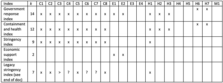
| Containment and closure | |
| C1 | School closing |
| C2 | Workplace closing |
| C3 | Cancel public events |
| C4 | Restrictions on gathering size |
| C5 | Close public transport |
| C6 | Stay at home requirements |
| C7 | Restrictions on internal movement |
| C8 | Restrictions on international travel |
| Economic response | |
| E1 | Income support |
| E2 | Debt/contract relief for households |
| E3 | Fiscal measures |
| E4 | Giving international support |
| Health systems | |
| H1 | Public information campaign |
| H2 | Testing policy |
| H3 | Contact tracing |
| H4 | Emergency investment in healthcare |
| H5 | Investment in COVID-19 vaccines |
| H6 | Facial coverings |
| H7 | Vaccination Policy |
| Overall indices | |
 | |
| Harris and Tzavalis (1999) test statistics: | |||
| Ho | Panels contain unit roots | Number of panels = 80 | |
| Ha | Panels are stationary | Number of periods = 52 | |
| AR parameter: Common | Asymptotics: N -> Infinity | ||
| Panel means: Included | T Fixed | ||
| Time trend: Not included | |||
| Test Statistic | z | p-value | |
| g_cases100k | 0.9292 | −2.1264 | 0.0167 |
| g_deaths100k | 0.9265 | −2.5296 | 0.0057 |
| econsupport | 0.9299 | −2.2308 | 0.0128 |
| stringency | 0.9161 | −4.3313 | 0.0000 |
Appendix B
| VARIABLES | March | April | May | June | July | August |
| L.market_RSI | −0.744 *** | −0.447 ** | −0.312 ** | −0.260 | −0.325 ** | 0.082 |
| (0.152) | (0.172) | (0.138) | (0.201) | (0.131) | (0.257) | |
| g_cases100k | 13.718 | −20.311 ** | 1.529 | 0.130 | −0.841 * | 1.020 |
| (8.696) | (8.069) | (4.515) | (4.215) | (0.401) | (1.194) | |
| L.g_cases100k | −142.701 ** | −8.377 * | 1.622 | 1.039 | 0.469 | −0.607 |
| (55.279) | (3.831) | (5.176) | (6.444) | (0.783) | (0.420) | |
| g_deaths100k | 480.140 *** | 235.157 ** | 86.765 | 32.621 | 35.143 | 15.499 |
| (120.150) | (90.527) | (180.701) | (56.367) | (30.337) | (69.784) | |
| L.g_deaths100k | −5412.173 ** | 300.498 | −472.027 ** | −68.911 | −5.399 | −7.206 |
| (1762.566) | (226.469) | (157.446) | (49.951) | (11.942) | (30.337) | |
| stringency | 0.236 | −0.745 | 0.221 | 0.409 | −0.628 | 2.002 |
| (0.172) | (1.432) | (0.466) | (0.450) | (1.750) | (3.224) | |
| econsupport | 0.619 ** | 0.199 | 1.348 ** | 0.932 *** | N.A. | 1.608 *** |
| (0.201) | (0.250) | (0.504) | (0.262) | (0.356) | ||
| Constant | 52.978 *** | 128.909 | −20.634 | −31.262 | 96.370 | −169.473 |
| (8.476) | (116.183) | (49.962) | (38.554) | (96.676) | (201.462) | |
| Observations | 44 | 44 | 55 | 44 | 55 | 44 |
| R-squared | 0.497 | 0.384 | 0.247 | 0.123 | 0.232 | 0.192 |
| VARIABLES | September | October | November | December | Overall | |
| L.market_RSI | −0.497 *** | −0.353 *** | −0.248 *** | 0.223 | −0.080 * | |
| (0.082) | (0.106) | (0.074) | (0.208) | (0.044) | ||
| g_cases100k | −0.864 *** | −0.129 | −0.229 | −0.538 | −0.077 | |
| (0.222) | (0.253) | (0.461) | (0.416) | (0.190) | ||
| L.g_cases100k | 2.892 *** | −0.441 *** | −0.200 | 0.165 | 0.079 | |
| (0.510) | (0.087) | (0.403) | (0.253) | (0.182) | ||
| g_deaths100k | 75.342 *** | 0.205 | −0.440 | 63.061 ** | 6.573 | |
| (22.311) | (10.781) | (5.295) | (27.461) | (5.506) | ||
| L.g_deaths100k | −113.612 *** | −23.332 ** | −5.711 | −51.258 ** | −4.990 | |
| (29.899) | (7.574) | (6.054) | (19.772) | (5.239) | ||
| stringency | −0.224 | 0.723 | −0.664 | 1.773 | 0.113 ** | |
| (0.335) | (0.834) | (1.975) | (1.053) | (0.043) | ||
| econsupport | −0.044 | −0.053 | −0.321 ** | N.A. | 0.004 | |
| (0.175) | (0.322) | (0.109) | (0.037) | |||
| Constant | 65.039 ** | 34.532 | 127.520 | −58.046 | 39.884 *** | |
| (24.355) | (42.385) | (115.204) | (52.808) | (3.485) | ||
| Observations | 44 | 55 | 44 | 55 | 561 | |
| R-squared | 0.456 | 0.220 | 0.204 | 0.198 | 0.026 |
| March | April | May | June | July | August | |
| L.market_RSI | −0.530 * | −0.536 *** | −0.294 ** | 0.110 | −0.165 | −0.299 ** |
| (0.254) | (0.097) | (0.117) | (0.140) | (0.122) | (0.097) | |
| g_cases100k | −4.509 | −1.108 | −0.701 | −3.563 *** | 1.280 * | 0.995 * |
| (2.679) | (0.941) | (0.488) | (1.087) | (0.665) | (0.520) | |
| L.g_cases100k | 3.252 | 2.896 | −0.116 | 3.816 *** | −0.122 | −1.329 ** |
| (2.168) | (2.244) | (0.583) | (1.172) | (1.088) | (0.554) | |
| g_deaths100k | −116.483 | −123.979 | −109.811 | 476.655 | 110.931 | 24.827 |
| (300.361) | (106.059) | (240.260) | (415.277) | (117.489) | (83.461) | |
| L.g_deaths100k | −792.754 ** | 226.992 | 253.016 | 267.141 | −4.059 | 165.591 |
| (303.131) | (196.603) | (305.944) | (247.474) | (75.972) | (181.660) | |
| stringency | 0.572 *** | −0.566 | 0.105 | −0.467 | 0.904 | 3.805 |
| (0.135) | (0.475) | (0.462) | (0.490) | (0.529) | (3.612) | |
| econsupport | 0.164 | 0.070 | 0.247 | N.A. | 0.675 | N.A. |
| (0.395) | (0.305) | (0.441) | (0.496) | |||
| Constant | 29.941 ** | 84.926 ** | 36.648 | 41.930 | −47.830 | −171.266 |
| (11.627) | (35.623) | (32.772) | (29.311) | (34.670) | (211.734) | |
| Observations | 44 | 44 | 55 | 44 | 55 | 44 |
| R−squared | 0.357 | 0.563 | 0.166 | 0.309 | 0.169 | 0.217 |
| VARIABLES | September | October | November | December | Overall | |
| L.market_RSI | −0.395 *** | −0.409 *** | −0.404 *** | −0.130 | −0.102 ** | |
| (0.069) | (0.105) | (0.093) | (0.089) | (0.045) | ||
| g_cases100k | −1.271 | 3.423 ** | 2.395 | −0.037 | 0.393 ** | |
| (4.036) | (1.138) | (2.120) | (2.640) | (0.128) | ||
| L.g_cases100k | −1.583 | −7.571 *** | −5.564 ** | 7.108 ** | −0.193 | |
| (2.304) | (0.837) | (2.488) | (3.070) | (0.109) | ||
| g_deaths100k | 92.402 | 209.814 *** | −267.268 * | −34.593 | 18.023 | |
| (72.386) | (26.199) | (136.796) | (121.723) | (12.643) | ||
| L.g_deaths100k | 20.187 | 379.406 *** | −519.049 ** | −283.198 ** | −30.654 * | |
| (57.935) | (47.946) | (230.209) | (111.966) | (14.542) | ||
| stringency | −1.394 ** | −0.192 | −0.544 | 0.634 | −0.120* | |
| (0.470) | (0.580) | (0.319) | (0.995) | (0.064) | ||
| econsupport | −0.838 * | 0.075 | −1.044 *** | N.A. | −0.013 | |
| (0.445) | (0.272) | (0.279) | (0.031) | |||
| Constant | 185.791 *** | 30.843 | 207.107 *** | −18.009 | 50.157 *** | |
| (42.899) | (17.288) | (39.709) | (60.508) | (3.483) | ||
| Observations | 44 | 55 | 44 | 55 | 561 | |
| R−squared | 0.378 | 0.310 | 0.544 | 0.237 | 0.028 |
| VARIABLES | March | April | May | June | July | August |
| L.market_RSI | −0.428 *** | −0.468 *** | −0.248 ** | −0.218 | −0.428 *** | −0.335 *** |
| (0.099) | (0.118) | (0.112) | (0.183) | (0.140) | (0.112) | |
| g_cases100k | −0.181 | 1.574 | −0.834 | 3.445 ** | −0.570 | −1.938 * |
| (1.416) | (0.942) | (0.886) | (1.261) | (1.718) | (0.960) | |
| L.g_cases100k | 0.620 | −0.639 | 0.022 | −1.218 | −1.718 | 3.280 ** |
| (1.678) | (0.908) | (0.573) | (1.402) | (2.570) | (1.483) | |
| g_deaths100k | −15.519 | −28.022 | 22.677 | −19.849 | 29.426 | −6.398 |
| (24.565) | (21.217) | (26.760) | (61.024) | (77.903) | (35.036) | |
| L.g_deaths100k | −656.247 ** | 11.441 | 4.998 | −38.381 | 22.175 | −6.396 |
| (254.080) | (15.646) | (24.329) | (70.173) | (50.650) | (29.155) | |
| stringency | 0.202 | 0.716 | 0.205 | 1.188 ** | 0.486 | −2.348 |
| (0.199) | (0.928) | (0.345) | (0.412) | (0.682) | (1.681) | |
| econsupport | 0.109 | −0.094 | −0.213 ** | −0.622 | −0.326 | −1.406 *** |
| (0.193) | (0.346) | (0.091) | (0.411) | (0.551) | (0.399) | |
| Constant | 46.634 *** | 4.741 | 46.776 ** | 30.250 | 68.592 | 241.655 *** |
| (5.823) | (72.788) | (20.599) | (42.737) | (66.061) | (43.420) | |
| Observations | 60 | 60 | 75 | 60 | 75 | 60 |
| R-squared | 0.299 | 0.299 | 0.105 | 0.244 | 0.227 | 0.290 |
| VARIABLES | September | October | November | December | Overall | |
| L.market_RSI | −0.363 ** | −0.341 ** | −0.068 | −0.226 | −0.087 ** | |
| (0.123) | (0.121) | (0.100) | (0.137) | (0.032) | ||
| g_cases100k | 0.675 | 0.290 *** | 0.004 | 0.042 | 0.054 | |
| (0.935) | (0.080) | (0.057) | (0.042) | (0.039) | ||
| L.g_cases100k | −0.071 | −0.635 ** | 0.055 | −0.093 | −0.048 | |
| (1.039) | (0.250) | (0.067) | (0.078) | (0.040) | ||
| g_deaths100k | 42.726 | 6.618 | −8.207 | 0.702 | −0.810 | |
| (36.303) | (11.298) | (4.938) | (3.306) | (2.483) | ||
| L.g_deaths100k | −53.162 | −2.505 | 5.420 | −0.064 | 0.210 | |
| (31.399) | (9.568) | (5.000) | (1.879) | (2.215) | ||
| stringency | 0.104 | 0.420 | −0.178 | 0.195 | −0.047 | |
| (0.857) | (0.572) | (0.769) | (0.575) | (0.039) | ||
| econsupport | 0.338 | 0.729 | 0.441 ** | 0.179 | 0.030 | |
| (0.349) | (0.418) | (0.180) | (0.599) | (0.026) | ||
| Constant | 22.225 | 4.157 | 26.000 | 31.965 | 45.128 *** | |
| (63.869) | (37.693) | (36.055) | (59.332) | (2.753) | ||
| Observations | 60 | 75 | 60 | 75 | 765 | |
| R-squared | 0.283 | 0.258 | 0.141 | 0.098 | 0.018 |
| VARIABLES | March | April | May | June | July | August |
| L.market_RSI | −0.670 *** | −0.203 | −0.266 *** | −0.410 * | −0.204 | −0.162 |
| (0.078) | (0.226) | (0.078) | (0.206) | (0.113) | (0.184) | |
| g_cases100k | 10.573 | −1.421 | 0.151 | 0.473 | 0.279 | 0.729 * |
| (11.344) | (1.577) | (0.527) | (0.564) | (0.857) | (0.368) | |
| L.g_cases100k | −18.246 | 1.166 | 0.047 | 0.364 | 0.093 | 0.285 |
| (36.549) | (3.572) | (0.605) | (0.726) | (0.470) | (0.620) | |
| g_deaths100k | 97.397 | 23.488 | 12.702 | 0.780 | −2.405 | 1.690 |
| (191.826) | (14.754) | (47.466) | (10.623) | (2.878) | (2.042) | |
| L.g_deaths100k | 1305.017 *** | 15.234 | −18.446 | 22.164 * | −4.318 * | 1.667 |
| (299.437) | (14.131) | (46.832) | (11.818) | (1.917) | (1.707) | |
| stringency | −0.167 | 0.117 | −0.411 | 1.919 ** | 1.623 | −1.604 |
| (0.266) | (0.189) | (0.644) | (0.675) | (1.082) | (1.380) | |
| econsupport | 0.072 | 1.024 | −1.503 *** | −1.496 * | 0.163 *** | −0.738 * |
| (0.202) | (0.840) | (0.191) | (0.763) | (0.014) | (0.361) | |
| Constant | 79.437 *** | −7.653 | 159.103 ** | −76.639 | −82.996 | 137.262 |
| (9.885) | (38.750) | (60.377) | (65.775) | (81.419) | (75.742) | |
| Observations | 40 | 40 | 50 | 40 | 50 | 40 |
| R-squared | 0.404 | 0.186 | 0.108 | 0.419 | 0.153 | 0.153 |
| VARIABLES | September | October | November | December | Overall | |
| L.market_RSI | −0.276 ** | −0.341 ** | 0.027 | −0.211 | −0.065 | |
| (0.121) | (0.107) | (0.080) | (0.164) | (0.051) | ||
| g_cases100k | −0.685 | −0.900 ** | 0.658 | 0.689 * | −0.187 | |
| (0.553) | (0.350) | (0.378) | (0.375) | (0.133) | ||
| L.g_cases100k | −0.424 | 0.560 | −1.352 * | 0.225 | 0.173 | |
| (0.378) | (0.398) | (0.666) | (0.289) | (0.133) | ||
| g_deaths100k | −16.887 ** | −0.590 | −1.091 | −13.964 | −0.380 | |
| (6.769) | (3.509) | (17.140) | (11.587) | (0.481) | ||
| L.g_deaths100k | 10.618 | −1.719 | 41.564 ** | 26.028 | −1.011 | |
| (13.972) | (1.916) | (17.820) | (16.944) | (0.554) | ||
| stringency | 0.451 | 1.211 | −0.641 | −1.847 | −0.018 | |
| (3.357) | (1.438) | (4.114) | (1.238) | (0.052) | ||
| econsupport | N.A. | 0.546 | 1.940 | 0.010 | −0.020 | |
| (0.384) | (1.178) | (0.199) | (0.048) | |||
| Constant | 109.093 | −36.296 | −51.570 | 102.468 | 50.040 *** | |
| (235.789) | (90.164) | (211.930) | (90.198) | (3.678) | ||
| Observations | 40 | 50 | 40 | 50 | 510 | |
| R-squared | 0.368 | 0.345 | 0.380 | 0.273 | 0.021 |
| VARIABLES | March | April | May | June | July | August |
| L.market_RSI | −0.568 *** | −0.346 ** | −0.304 ** | −0.393 ** | −0.451 *** | −0.373 ** |
| (0.119) | (0.125) | (0.136) | (0.146) | (0.064) | (0.146) | |
| g_cases100k | −1.833 *** | 0.307 | −0.116 | 0.206 | 0.036 | −0.095 |
| (0.311) | (0.228) | (0.089) | (0.276) | (0.170) | (0.304) | |
| L.g_cases100k | −6.225 *** | −0.500 | 0.079 | −0.414 | 0.078 | −0.003 |
| (1.282) | (0.530) | (0.097) | (0.337) | (0.110) | (0.274) | |
| g_deaths100k | 301.004 *** | −43.091 | 51.445 *** | 29.386 | −18.239 * | 41.388 * |
| (93.478) | (85.319) | (10.123) | (29.490) | (8.716) | (21.533) | |
| L.g_deaths100k | −304.246 | 16.517 | −23.748 | −15.818 | −1.660 | 21.193 |
| (370.710) | (47.538) | (16.573) | (22.477) | (7.496) | (32.716) | |
| stringency | 0.239 | 1.535 | −2.735 *** | 5.126 *** | −0.288 | −0.470 |
| (0.187) | (1.493) | (0.549) | (1.428) | (0.623) | (0.448) | |
| econsupport | −0.153 | 0.017 | 1.214 *** | N.A. | 0.205 | 2.043 *** |
| (0.489) | (0.398) | (0.312) | (0.181) | (0.310) | ||
| Constant | 60.284 *** | −74.888 | 211.773 *** | −322.243 ** | 68.880 | −77.688 ** |
| (9.090) | (139.403) | (52.258) | (110.870) | (50.708) | (28.648) | |
| Observations | 48 | 48 | 60 | 48 | 60 | 48 |
| R-squared | 0.391 | 0.139 | 0.338 | 0.243 | 0.239 | 0.232 |
| VARIABLES | September | October | November | December | Overall | |
| L.market_RSI | −0.481 *** | −0.376 *** | −0.147 | −0.177 | −0.091 ** | |
| (0.136) | (0.092) | (0.152) | (0.228) | (0.038) | ||
| g_cases100k | 0.578 *** | 0.085 | 0.316 | −0.008 | 0.003 | |
| (0.171) | (0.134) | (0.210) | (0.011) | (0.012) | ||
| L.g_cases100k | −0.256 ** | −0.216 ** | −0.426 | −0.028 *** | −0.029 ** | |
| (0.105) | (0.089) | (0.340) | (0.009) | (0.010) | ||
| g_deaths100k | −55.666 | 4.572 | 8.720 | −24.143 | 7.230 | |
| (46.227) | (19.869) | (9.381) | (16.088) | (5.575) | ||
| L.g_deaths100k | 11.466 | −12.941 | −2.006 | −3.493 | −7.233 * | |
| (48.205) | (26.220) | (8.550) | (25.960) | (3.677) | ||
| stringency | −1.780 *** | 0.828 | 0.119 | −0.874 | 0.020 | |
| (0.349) | (0.553) | (0.221) | (0.546) | (0.036) | ||
| econsupport | N.A. | −0.267 | −0.322 ** | −0.584* | 0.038 | |
| (0.472) | (0.126) | (0.288) | (0.041) | |||
| Constant | 159.008 *** | 36.473 ** | 70.664 *** | 153.390 *** | 42.441 *** | |
| (17.888) | (15.050) | (20.417) | (24.035) | (2.432) | ||
| Observations | 48 | 60 | 48 | 60 | 612 | |
| R-squared | 0.484 | 0.230 | 0.208 | 0.168 | 0.018 |
| VARIABLES | March | April | May | June | July | August |
| L.market_RSI | −0.498 *** | −0.483 *** | −0.117 | −0.319 *** | −0.107 | −0.379 *** |
| (0.096) | (0.140) | (0.074) | (0.109) | (0.076) | (0.039) | |
| g_cases100k | −0.114 | 0.147 | 1.694 | 5.975 ** | 1.064 *** | 0.136 ** |
| (0.265) | (0.091) | (1.237) | (2.200) | (0.346) | (0.059) | |
| L.g_cases100k | 0.025 | −0.135 * | −0.880 | −4.796 *** | 0.033 | −0.253 |
| (0.420) | (0.073) | (0.835) | (1.393) | (0.167) | (0.325) | |
| g_deaths100k | −0.891 | −3.102 *** | 7.139 *** | −6.858 | −114.578 *** | 10.443 |
| (3.503) | (0.698) | (2.252) | (6.785) | (30.085) | (7.862) | |
| L.g_deaths100k | −12.493 * | 3.020 ** | −3.941 | 2.587 | 28.716 | 35.886 |
| (7.105) | (1.257) | (5.521) | (4.790) | (34.079) | (33.406) | |
| stringency | −0.207 | −1.897 | −0.459 | −0.571 | 0.229 | 0.408 |
| (0.154) | (1.118) | (0.452) | (0.341) | (0.541) | (0.344) | |
| econsupport | −0.158 | −0.554 *** | 1.402 ** | N.A. | −0.272 | N.A. |
| (0.102) | (0.099) | (0.561) | (0.302) | |||
| Constant | 85.220 *** | 250.937 ** | −45.938 | 74.225 *** | 46.982 | 26.006 |
| (6.609) | (87.328) | (35.082) | (22.815) | (29.883) | (16.776) | |
| Observations | 68 | 68 | 85 | 68 | 85 | 68 |
| R-squared | 0.457 | 0.449 | 0.109 | 0.222 | 0.233 | 0.306 |
| VARIABLES | September | October | November | December | Overall | |
| L.market_RSI | −0.410 *** | −0.214 *** | −0.163 * | −0.396 *** | −0.160 *** | |
| (0.085) | (0.061) | (0.085) | (0.108) | (0.029) | ||
| g_cases100k | 0.004 | 0.080 | −0.052 | −0.043 | 0.051 *** | |
| (0.317) | (0.048) | (0.055) | (0.045) | (0.009) | ||
| L.g_cases100k | 0.176 ** | −0.034 | −0.026 | 0.021 | −0.059 *** | |
| (0.061) | (0.108) | (0.053) | (0.066) | (0.015) | ||
| g_deaths100k | −8.524 | −3.357 | 4.042 * | 3.119 | −1.251 ** | |
| (17.846) | (4.885) | (2.225) | (4.030) | (0.544) | ||
| L.g_deaths100k | 6.475 | 19.665 *** | −3.714 * | −4.854 * | 1.861 *** | |
| (17.787) | (6.074) | (1.775) | (2.395) | (0.378) | ||
| stringency | 0.173 | 0.121 | 0.829 | −0.863 * | −0.025 | |
| (0.948) | (0.483) | (1.213) | (0.476) | (0.056) | ||
| econsupport | −0.214 | −0.267 | −0.075 | −0.886 *** | −0.060 | |
| (0.407) | (0.390) | (0.479) | (0.103) | (0.041) | ||
| Constant | 62.757 | 44.764 | 5.512 | 189.460 *** | 49.459 *** | |
| (55.013) | (35.564) | (105.188) | (28.876) | (2.153) | ||
| Observations | 68 | 85 | 68 | 85 | 867 | |
| R-squared | 0.183 | 0.311 | 0.125 | 0.196 | 0.045 |
| 1 | This is itself consistent with the past experiences considered by Friedman (2005), who links the US stock market recovery from the post-1999 crash to rapid Federal Reserve monetary expansion and contrasts this with the effects of stagnant money supply in post-1989 Japan and monetary contraction in the post-1929 US case. Meanwhile, as with the late 1990s Nasdaq bubble, the effects of US monetary expansion in 2020–2021 may well have been channeled primarily into the stock market (whereas goods prices remained subdued). |
| 2 | An especially telling fact is Velde’s (2020) observation that, by the January 1919 issue of the Federal Reserve Bulletin, the Spanish Flu pandemic was no longer meriting even a mention in the Federal Reserve’s main publication. The contrast with the aftermath of the coronavirus pandemic in 2021 could not be more stark. |
| 3 | The onset of such high volatility regimes can itself produce significant sectoral effects, as seen in Burdekin and Tao’s (2021) comparative Markov-switching analysis of gold’s hedging value in 2020 vs. 2008–2009. |
| 4 | |
| 5 | Similarly, whereas contagion often emerged during past European crises, Boţoc and Anton (2020) find that this typically proved to to be a short-lived phenomenon and was not necessarily indicative of greater longer-run cointegration. |
| 6 | Further evidence on the differential stock market reactions around this time is provided by Mazur et al. (2021), who, not surprisingly, find widespread sectoral variations. |
| 7 | Not only does experience from past pandemics suggest considerable risks of post-pandemic inflation owing to pent-up consumer demand (Burdekin 2020a), but also such dangers have likely been greatly understated by Modern Monetary Theory proponents (see Bird et al. 2021). |
| 8 | Few countries outside of China exhibited meaningful virus case numbers and deaths prior to March. |
| 9 | Dollar returns, rather than returns in local currency, allows for more of an apples-to-apples comparison as the gains in value of a dollar invested in the US market are set against the gains realized from that same dollar invested abroad. |
| 10 | Stationarity of the variables entered in the regressions is confirmed by application of the Harris and Tzavalis (1999) unit root test. This test is appliable to cases where the number of panels is large relative to the number of time periods. The results reject the presence of a unit root at better than the 98% confidence level or better in each case (Appendix A Table A3). |
References
- Al-Awadhi, Abdullah Khaled Alsaifi, Ahmad Al-Awadhi, and Salah Alhammadi. 2020. Death and contagious infectious diseases: Impact of the COVID-19 virus on stock market returns. Journal of Behavioral and Experimental Finance 27: 100326. [Google Scholar] [CrossRef] [PubMed]
- Alber, Nader. 2020. The Effect of Coronavirus Spread on Stock Markets: The Case of the Worst 6 Countries. Available online: https://ssrn.com/abstract=3578080 (accessed on 10 April 2021).
- Ashraf, Badar Nadeem. 2020. Stock markets’ reaction to COVID-19: Cases or fatalities? Research in International Business and Finance 54: 101249. [Google Scholar] [CrossRef]
- Ashraf, Badar Nadeem. 2021. Stock markets’ reaction to COVID-19: Moderating role of national culture. Finance Research Letters. forthcoming. [Google Scholar]
- Baker, Scott R., Nicholas Bloom, Steven J. Davis, Kyle J. Kost, Marco C. Sammon, and Tasaneeya Viratyosin. 2020. The Unprecedented Stock Market Impact of COVID-19. Working Paper 26945. Cambridge, MA: National Bureau of Economic Research. [Google Scholar]
- Bird, Graham, Eric Pentecost, and Thomas Willett. 2021. Modern Monetary Theory and the policy response to COVID-19: Old wine in new bottles. World Economy. forthcoming. [Google Scholar]
- Boţoc, Claudio, and Sorin Gabriel Anton. 2020. New empirical evidence on CEE’s stock markets integration. World Economy 43: 2785–802. [Google Scholar] [CrossRef]
- Burdekin, Richard C. K. 2020a. The money explosion of 2020, monetarism and inflation: Plagued by history? Modern Economy 11: 1887–900. [Google Scholar] [CrossRef]
- Burdekin, Richard C. K. 2020b. Economic and financial effects of the 1918–1919 Spanish Flu pandemic. Journal of Infectious Diseases & Therapy 8: 1000439. [Google Scholar]
- Burdekin, Richard C. K. 2021. Death and the stock market: International evidence from the Spanish Flu. Applied Economics Letters. forthcoming. [Google Scholar]
- Burdekin, Richard C. K., and Ran Tao. 2021. The golden hedge: From global financial crisis to global pandemic. Economic Modelling 95: 170–80. [Google Scholar] [CrossRef]
- Chan-Lau, Jorge A., and Yunhui Zhao. 2020. Hang in There: Stock Market Reactions to Withdrawals of COVID-19 Stimulus Measures. Working Paper 20/285. Washington, DC: International Monetary Fund. [Google Scholar]
- Cox, Josue, Daniel L. Greenwald, and Sydney C. Ludvigson. 2020. What Explains the COVID-19 Stock Market? Working Paper 27784. Cambridge, MA: National Bureau of Economic Research. [Google Scholar]
- Friedman, Milton. 2005. A natural experiment in monetary policy covering three episodes of growth and decline in the economy and the stock market. Journal of Economic Perspectives 19: 145–50. [Google Scholar] [CrossRef]
- Greenwood, John, and Steve H. Hanke. 2021. The money boom is already here. Available online: https://www.wsj.com/articles/the-money-boom-is-already-here-11613944730 (accessed on 10 April 2021).
- Hale, Thomas, Noam Angrist, Thomas Boby, Emily Cameron-Blake, Laura Hallas, Beatriz Kira, Saptarshi Majumdar, Anna Petherick, Toby Phillips, Helen Tatlow, and et al. 2020. Variation in Government Responses to COVID-19. Working Paper 2020/032. Oxford, UK: Blavatnik School of Government, Oxford University. [Google Scholar]
- Harjoto, Maretno Agus, Fabrizio Rossi, and John K. Paglia. 2021. COVID-19: Stock market reactions to the shock and the stimulus. Applied Economics Letters. forthcoming. [Google Scholar]
- Harris, Richard D. F., and Elias Tzavalis. 1999. Inference for unit roots in dynamic panels where the time dimension is fixed. Journal of Econometrics 91: 201–26. [Google Scholar] [CrossRef]
- Just, Malgorzata, and Krzystof Echaust. 2020. Stock market returns, volatility, correlation and liquidity during the COVID-19 crisis: Evidence from the Markov switching approach. Finance Research Letters 37: 101775. [Google Scholar] [CrossRef] [PubMed]
- Khan, Karamat, Huawei Zhao, Han Zhang, Huilin Yang, Muhammad Haroon Shah, and Atif Jahanger. 2020. The impact of COVID-19 pandemic on stock markets: An empirical analysis of world major stock indices. Journal of Asian Finance, Economics, and Business 7: 463–74. [Google Scholar] [CrossRef]
- Magalhaes, Luciana, and Samantha Pearson. 2020. Brazil’s president promised economic change: Now he is writing Covid−19 relief checks. Available online: https://www.wsj.com/articles/brazils-president-promised-economic-change-now-he-is-writing-covid-19-relief-checks-11605186008 (accessed on 10 April 2021).
- Malnick, Edward. 2020. Boris Johnson exclusive interview: We will not need another national lockdown. Available online: https://www.telegraph.co.uk/politics/2020/07/18/boris-johnson-exclusive-interview-will-not-need-another-national/ (accessed on 10 April 2021).
- Mazur, Mieszko, Man Dang, and Miguel Vega. 2021. COVID-19 and the March 2020 stock market crash. Evidence from S&P1500. Finance Research Letters 38: 101690. [Google Scholar] [PubMed]
- Okorie, David Iheke, and Boqiang Lin. 2021. Stock markets and the COVID-19 fractal contagion effects. Finance Research Letters 38: 101640. [Google Scholar] [CrossRef] [PubMed]
- Phan, Dinh Hoang Bach, and Paresh Kumar Narayan. 2020. Country responses and the reaction of the stock market to COVID-19—A preliminary exposition. Emerging Markets Finance and Trade 56: 2138–50. [Google Scholar] [CrossRef]
- Rahman, Md Lutfur, Abu Amin, and Mohammed Abdullah Al Mamun. 2021. The COVID-19 outbreak and stock market reactions: Evidence from Australia. Finance Research Letters 38: 101832. [Google Scholar] [CrossRef]
- Testa, Christian C., Nancy Krieger, Jarvis T. Chen, and William P. Hanage. 2020. Visualizing the Lagged Connection between COVID-19 Cases and Deaths in the United States: An Animation Using Per Capita State-Level Data (January 22, 2020–July 8, 2020). Working Paper 19(4). Cambridge, MA: Harvard Center for Population and Development Studies. [Google Scholar]
- Velde, François R. 2020. What Happened to the US Economy during the 1918 Influenza Pandemic? A View through High-Frequency Data. WP 2020-11, Federal Reserve Bank of Chicago. Available online: https://www.chicagofed.org/publications/working-papers/2020/2020-11 (accessed on 10 April 2021).
| a. Full Sample | |||||
| count | mean | sd | min | max | |
| market_RSI | 4240 | 40.5 | 23.09493 | 1 | 80 |
| g_cases100k | 4160 | 41.44165 | 90.85629 | −179.5596 | 1203.091 |
| g_deaths100k | 4160 | 0.7668794 | 1.798592 | −3.2232 | 18.49932 |
| stringency | 4240 | 51.30944 | 27.16211 | 0 | 100 |
| econsupport | 4240 | 48.98585 | 34.41286 | 0 | 100 |
| b. Africa | |||||
| count | mean | sd | min | max | |
| market_RSI | 583 | 42.48885 | 23.49986 | 1 | 80 |
| g_cases100k | 572 | 9.616895 | 22.52485 | 0 | 146.5333 |
| g_deaths100k | 572 | 0.2194387 | 0.6140417 | 0 | 5.347495 |
| stringency | 583 | 48.40607 | 28.56593 | 0 | 93.52 |
| econsupport | 583 | 37.92882 | 32.34679 | 0 | 100 |
| c. Australasia | |||||
| count | mean | Sd | min | max | |
| market_RSI | 106 | 37.76415 | 21.59345 | 2 | 78 |
| g_cases100k | 104 | 1.502934 | 2.912689 | 0 | 13.40398 |
| g_deaths100k | 104 | 0.0392611 | 0.100428 | −0.0039216 | 0.5803949 |
| stringency | 106 | 44.64877 | 26.9876 | 0 | 96.3 |
| econsupport | 106 | 60.14151 | 32.5555 | 0 | 100 |
| d. East Asia | |||||
| count | mean | sd | min | max | |
| market_RSI | 583 | 39.4837 | 21.63178 | 1 | 80 |
| g_cases100k | 572 | 4.373834 | 11.17784 | 0 | 120.0784 |
| g_deaths100k | 572 | 0.0442898 | 0.0892606 | 0 | 0.6588728 |
| stringency | 583 | 50.63443 | 23.04173 | 0 | 100 |
| econsupport | 583 | 46.93396 | 34.95796 | 0 | 100 |
| e. Eastern and Southern Europe | |||||
| count | mean | sd | min | max | |
| market_RSI | 795 | 40.54591 | 21.73602 | 1 | 80 |
| g_cases100k | 780 | 57.9161 | 117.8906 | −0.4040714 | 748.3035 |
| g_deaths100k | 780 | 1.123939 | 2.549789 | −0.4523048 | 17.31658 |
| stringency | 795 | 46.34185 | 26.29474 | 0 | 96.3 |
| econsupport | 795 | 53.01887 | 33.15399 | 0 | 100 |
| f. Latin America | |||||
| count | mean | sd | min | max | |
| market_RSI | 530 | 42.88679 | 26.56565 | 1 | 80 |
| g_cases100k | 520 | 36.31582 | 51.12816 | 0 | 246.3407 |
| g_deaths100k | 520 | 1.13994 | 1.776847 | 0 | 15.79226 |
| stringency | 530 | 58.97732 | 30.16572 | 0 | 100 |
| econsupport | 530 | 41.58019 | 32.50223 | 0 | 100 |
| g. North America | |||||
| count | mean | sd | min | max | |
| market_RSI | 106 | 37.73585 | 18.72778 | 7 | 74 |
| g_cases100k | 104 | 72.89453 | 102.6356 | 0 | 463.8697 |
| g_deaths100k | 104 | 1.402589 | 1.410535 | 0 | 5.45615 |
| stringency | 106 | 54.84009 | 26.07422 | 0 | 75.46 |
| econsupport | 106 | 53.89151 | 29.04037 | 0 | 75 |
| h. South Asia and Middle East | |||||
| count | mean | Sd | min | max | |
| market_RSI | 636 | 40.47956 | 23.21433 | 1 | 80 |
| g_cases100k | 624 | 51.01512 | 86.15512 | 0 | 1203.091 |
| g_deaths100k | 624 | 0.3522827 | 0.4588852 | 0 | 2.98075 |
| stringency | 636 | 57.83392 | 28.00892 | 0 | 100 |
| econsupport | 636 | 44.65409 | 32.02359 | 0 | 100 |
| i. Western Europe | |||||
| count | mean | sd | min | max | |
| market_RSI | 901 | 39.08768 | 23.12896 | 1 | 80 |
| g_cases100k | 884 | 68.73868 | 123.657 | −179.5596 | 1075.221 |
| g_deaths100k | 884 | 1.357633 | 2.388899 | −3.2232 | 18.49932 |
| stringency | 901 | 49.26022 | 25.26129 | 0 | 93.52 |
| econsupport | 901 | 59.43396 | 36.13918 | 0 | 100 |
| VARIABLES | March | April | May | June | July | August |
| L.market_RSI | −0.502 *** | −0.407 *** | −0.234 *** | −0.253 *** | −0.259 *** | −0.228 *** |
| (0.044) | (0.055) | (0.039) | (0.064) | (0.043) | (0.050) | |
| g_cases100k | −0.334 | 0.161 ** | 0.074 | 0.220 | 0.115 | 0.174 *** |
| (0.289) | (0.064) | (0.094) | (0.194) | (0.127) | (0.054) | |
| L.g_cases100k | 0.068 | −0.220 *** | −0.037 | −0.296 | 0.127 | 0.140 |
| (0.487) | (0.051) | (0.107) | (0.242) | (0.116) | (0.168) | |
| g_deaths100k | −3.122 | −2.731 *** | 6.880 *** | 3.378 | −1.557 | 2.776 * |
| (4.282) | (0.651) | (2.172) | (3.498) | (2.377) | (1.526) | |
| L.g_deaths100k | −7.161 | 2.931 *** | −3.302 * | 7.889 ** | −3.632 ** | 2.213 * |
| (8.475) | (1.034) | (1.666) | (3.851) | (1.495) | (1.279) | |
| stringency | 0.161 *** | −0.275 | −0.025 | 0.117 | 0.640* | −0.371 |
| (0.060) | (0.333) | (0.161) | (0.254) | (0.381) | (0.274) | |
| econsupport | −0.144 * | −0.015 | 0.484 * | −0.058 | 0.104 | 0.106 |
| (0.073) | (0.142) | (0.244) | (0.420) | (0.200) | (0.588) | |
| Constant | 58.772 *** | 81.153 *** | 18.766 | 43.953 | 4.566 | 52.597 |
| (2.870) | (27.107) | (16.711) | (31.508) | (26.160) | (42.888) | |
| Observations | 320 | 320 | 400 | 320 | 400 | 320 |
| R-squared | 0.262 | 0.190 | 0.079 | 0.082 | 0.100 | 0.097 |
| VARIABLES | September | October | November | December | Overall | |
| L.market_RSI | −0.365 *** | −0.321 *** | −0.187 *** | −0.205 *** | −0.095 *** | |
| (0.040) | (0.037) | (0.038) | (0.056) | (0.016) | ||
| g_cases100k | 0.110 | 0.107 *** | 0.002 | −0.003 | 0.030 ** | |
| (0.131) | (0.039) | (0.048) | (0.011) | (0.012) | ||
| L.g_cases100k | 0.060 | −0.094 | −0.019 | −0.030 ** | −0.035 *** | |
| (0.108) | (0.075) | (0.036) | (0.011) | (0.011) | ||
| g_deaths100k | −18.080 *** | −2.859 | −0.086 | 1.273 | −0.627 | |
| (6.454) | (2.196) | (2.373) | (1.715) | (0.460) | ||
| L.g_deaths100k | −6.440 | 1.693 | −0.449 | −1.008 | 0.462 | |
| (8.296) | (3.115) | (2.157) | (1.499) | (0.478) | ||
| stringency | −1.070 *** | 0.158 | 0.190 | −0.241 | 0.006 | |
| (0.236) | (0.247) | (0.310) | (0.342) | (0.019) | ||
| econsupport | −0.114 | 0.228 | 0.053 | −0.612 *** | −0.018 | |
| (0.169) | (0.190) | (0.200) | (0.220) | (0.014) | ||
| Constant | 126.146 *** | 29.175 * | 36.922 | 104.391 *** | 45.238 *** | |
| (17.053) | (16.411) | (23.421) | (25.052) | (1.212) | ||
| Observations | 320 | 400 | 320 | 400 | 4080 | |
| R-squared | 0.193 | 0.136 | 0.061 | 0.059 | 0.013 |
Publisher’s Note: MDPI stays neutral with regard to jurisdictional claims in published maps and institutional affiliations. |
© 2021 by the authors. Licensee MDPI, Basel, Switzerland. This article is an open access article distributed under the terms and conditions of the Creative Commons Attribution (CC BY) license (https://creativecommons.org/licenses/by/4.0/).
Share and Cite
Burdekin, R.C.K.; Harrison, S. Relative Stock Market Performance during the Coronavirus Pandemic: Virus vs. Policy Effects in 80 Countries. J. Risk Financial Manag. 2021, 14, 177. https://doi.org/10.3390/jrfm14040177
Burdekin RCK, Harrison S. Relative Stock Market Performance during the Coronavirus Pandemic: Virus vs. Policy Effects in 80 Countries. Journal of Risk and Financial Management. 2021; 14(4):177. https://doi.org/10.3390/jrfm14040177
Chicago/Turabian StyleBurdekin, Richard C. K., and Samuel Harrison. 2021. "Relative Stock Market Performance during the Coronavirus Pandemic: Virus vs. Policy Effects in 80 Countries" Journal of Risk and Financial Management 14, no. 4: 177. https://doi.org/10.3390/jrfm14040177
APA StyleBurdekin, R. C. K., & Harrison, S. (2021). Relative Stock Market Performance during the Coronavirus Pandemic: Virus vs. Policy Effects in 80 Countries. Journal of Risk and Financial Management, 14(4), 177. https://doi.org/10.3390/jrfm14040177