Hybrid Machine Learning–Econometric Framework for Financial Distress Scoring: Evidence from German Manufacturing Firms

Abstract

Nowadays, the European economy faces significant global challenges that threaten the continuity of economic growth, especially in the German manufacturing sector, which is under strain from financial turmoil, resulting in numerous layoffs and firm closures. In this respect, FinTech significantly contributes to addressing these issues by providing data-driven analytical tools that improve the assessment and monitoring of firms’ financial position. However, in the literature, we have not found any paper that uses machine learning (ML) algorithms to assess the financial distress of German manufacturing firms, highlighting methodological and sectoral gaps that need to be bridged. Therefore, this study aims to develop an econometric and ML-based financial distress scoring model for German manufacturing firms by estimating contemporaneous Altman Z-scores that provide better insights into the financial distress determinants, enabling better financial management. The econometric findings revealed that the regression model has an adjusted R-squared value of 86%, confirming that the selected firm-specific and macroeconomic factors play a substantial role in explaining financial distress. The findings recommend that German manufacturing businesses retain more earnings rather than distributing them as dividends, while reducing their debt in capital structures to enhance financial stability. Moreover, the ML results found that Gradient Boosting and Random Forest have the highest accuracy scores among the ML methods, suggesting that these models provide strong capability for assessing financial distress and supporting more effective financial risk management, allowing firms to effectively respond to the threats of a dynamic environment and thereby better support the growth of the German and European economies.

1. Introduction

The continuity of good financial health is essential for the survival and growth of businesses. Aydin et al. (2022) [1] claimed that most studies indicate that financial firm-specific and macroeconomic variables are the primary determinants of financial distress. In other words, firm-specific factors such as liquidity, leverage, solvency, profitability, and management efficiency play a significant role in the financial stability of manufacturing firms, while external macroeconomic factors like GDP growth rate, inflation, interest rate, exchange rate, and unemployment rate mainly influence financial distress. In this context, manufacturing businesses require ongoing monitoring of their internal and external factors to improve their chances of survival and growth.

Dumitrescu et al. (2025) [2] stated that today, we live in a highly dynamic environment that necessitates integrating Artificial Intelligence (AI) into business models to enhance financial management performance, thereby achieving better financial outcomes that promote financial resilience within economies. In other words, Mallinguh and Zéman (2020) [3] argued that previous studies have demonstrated that businesses should utilize machine learning algorithms to enhance their assessment of financial distress, thereby strengthening their financial stability and reducing the risks of insolvency and bankruptcy.

Manufacturing companies play a vital role in the growth of the German economy, as their production significantly contributes to GDP growth. Furthermore, they hold a crucial and sensitive position in the development of Europe’s industrial powerhouse (Lohmann and Ohliger, 2020) [4]. However, today, Germany faces global challenges threatening its economic growth, as shown in Figure 1, due to surges in energy prices, increased US customs duties on imported goods, and fierce competition between China and Germany in the manufacturing sector. These challenges render the German manufacturing industry highly susceptible to global economic shocks and technological disruptions. Therefore, improving the accuracy of explaining financial distress in manufacturing enterprises through more advanced and sophisticated models, such as machine learning algorithms alongside traditional econometrics, is essential for enhancing financial risk management and better supporting survival and growth in a highly dynamic and challenging global environment (Dash and Dey, 2025) [5].

In this context, this study has plotted a graph illustrating how the Altman Z-score behaves from 2010 to 2024, which is used as a proxy for financial distress, as shown in Figure 2. From 2010 to 2018, the score remained relatively stable, averaging around 1.8, lower than 3. During the COVID-19 period, the score declined sharply and then recovered after 2020. However, from 2023 to 2024, the Z-score gradually fell below 1.8, indicating that most of the leading manufacturing firms were experiencing financial distress and require further investigation into the main causes of this decline. Meanwhile, the GDP growth rate, depicted in Figure 2, experienced a steep decrease during COVID-19, reaching −4.09%, before rebounding to 3.67%. Over the last three years, the GDP growth rate has been negative, signalling a recession.

Consequently, the ROA of these manufacturing firms has been gradually decreasing during 2023–2024, as illustrated in Figure 3, threatening their survival and growth—especially considering that these 21 top firms constitute most of Germany’s industrial output.

In this context, the purpose of this research is to model and evaluate the determinants of the contemporaneous Altman Z-score as a firm-level stability indicator. This model aligns with the architecture of modern FinTech by developing financial distress scoring models, which enhance interpretability and assist these firms in implementing better financial management strategies to support the recovery and growth of the German economy.

2. Literature Review and Hypotheses Development

This section focuses on reviewing the current literature on the determinants and prediction of financial distress in developed countries, which are classified as high-income countries by the World Bank, starting with theoretical studies, followed by empirical studies in developed countries, empirical studies in the rest of the world, the literature gap, and finally, hypothesis development.

2.1. Theoretical Studies

Financial distress occurs when companies face difficulties in repaying their debts. In other words, it arises when a firm has a high default risk, indicating that its earnings are insufficient to cover its debt obligations. The prediction of financial distress has been extensively studied in the literature using the Altman Z-score. Altman (1968) [6] developed this Z-score model to forecast financial distress among listed US manufacturing firms using Multiple Discriminant Analysis (MDA), and it has remained a widely accepted benchmark for such predictions. Additionally, Altman et al. (2017) [7] applied an updated version of the Z-score to assess its reliability in an international context across non-financial and mixed sectors, rather than being limited to the manufacturing sector, based on a sample from 31 European countries. The findings revealed that the accuracy reached 0.75 on average, but with country-specific analysis, accuracy can reach 0.90.

Furthermore, Altman (2018) [8] argued that the traditional Altman Z-score has been widely used as an early-warning model for predicting financial distress over the past 50 years, serving as the benchmark for credit risk measurement globally. Additionally, other studies have also demonstrated that this model is not only relevant to US manufacturing firms but also to other developed countries, such as those in Europe and Japan, showing that the traditional Altman Z-score remains valid and many businesses depend on it when assessing their financial risk exposures.

Furthermore, Bundesbank (2014) [9] utilized firm-specific data from the financial statements of German manufacturing companies to evaluate their impact on financial distress, employing the original Altman Z-score to enhance credit risk assessments by banks. The results indicated that traditional financial ratios significantly influence bankruptcy, emphasizing the relevance and validity of the original Z-score in predicting insolvency within the German manufacturing sector. In this context, this study selected the 1968 original Altman Z-score as a proxy for financial distress rather than the updated version, as it is tailored to the manufacturing sector, aligning with our research sample. In addition, Khoja et al. (2019) [10] illustrated the importance of using traditional financial ratios and macroeconomic indicators to predict financial distress in firms of the developed countries, such as the United Kingdom and the United States of America.

2.2. Empirical Studies in Developed Countries

In Italy, Amendola et al. (2015) [11] examined the determinants of financial distress, using a sample of Italian firms in the building sector with a panel dataset from 2004 to 2009. The econometric results showed that liquidity and inactivity significantly influence the financial distress of these firms. Boďa and Úradníček (2016) [12] evaluated the portability of two versions of the Altman Z-score, which were developed in 1986 and 1983 for non-listed manufacturing businesses in Slovakia. The findings revealed that both models can be used to predict the financial distress of the manufacturing firms in Slovakia. However, Ref. [13] used the Altman Z-score and GASIC to predict financial distress in the Spanish construction sector covering the period from 1995 to 2011. The results found that GASIC, which includes the financial ratios and macroeconomic variables, outperforms the prediction performance of the Altman model, highlighting the importance of these variables in enhancing the prediction of financial distress.

Altman et al. (2017) [7] employed multivariate discriminant analysis to evaluate the performance of the Altman Z-score model in predicting financial distress in manufacturing and non-manufacturing firms across 31 European countries. The results indicated that the model’s accuracy reached 90%, suggesting it can be effectively used to better predict financial risk exposure in businesses. In the United States, Inekwe et al. (2018) [14] explored the effect of financial distress on GDP growth rate over the period 1970–2012, and their findings revealed that the financial distress of US-based firms negatively impacts GDP growth, leading to lower levels of investment and exports.

Moreover, in Greece, Charalambakis and Garrett (2019) [15] investigated the determinants of financial distress by employing a multi-period logit model with a sample of 31,000 Greek private companies. The findings identified profitability, asset size, liquidity, firm growth potential, leverage, and GDP growth rate as the main influential factors. In Germany, Lohmann and Ohliger (2020) [4] explored whether characteristics of annual reports can help differentiate between bankrupt and solvent firms. They applied generalized linear models (GLMs) and other econometric techniques to a sample of 117 bankrupt and 117 solvent firms, using panel data from 2006 to 2016. Their findings revealed that common features in annual reports can distinguish these firms by analyzing textual elements and risk exposure explanations. However, financial ratio disclosures alone are insufficient for this purpose.

In Slovakia, Gregova et al. (2020) [16] utilized various machine learning algorithms such as ANNs, Random Forest, and Logistic Regression, using liquidity, activity, profitability, solvency, and leverage ratios as the independent variables. Based on the accuracy scores, they found that ANNs outperform the other traditional models. Furthermore, in Sweden, Yazdanfar and Öhman (2020) [17] employed regression analysis to investigate the determinants of financial distress using a sample of 3865 small and medium-sized enterprises (SMEs), based on panel data from 2008 to 2015. The results indicated that profitability, leverage, and the global financial crisis significantly influenced financial distress. Habib et al. (2020) [18] conducted a systematic review of the current literature and found that including firm-specific financial variables, such as profitability, liquidity, leverage, and cash flows, can enhance the prediction of financial distress in the businesses of developed countries.

Malakauskas and Lakštutienė (2021) [19] applied machine learning algorithms to predict the financial distress of the manufacturing firms, taking a sample of 12 thousand SMEs operating in the Baltic states and using the traditional financial ratios as the dependent variables of the models. The findings showed that the Random Forest model has the highest accuracy score over the Logistic Regression and artificial neural network (ANN) models. Ref. [20] employed a panel logit model to develop risk models combining accounting, macroeconomic, and stock market variables to predict the financial distress and bankruptcy of the listed firms operating in the United Kingdom and compared the performance against the neural network model and the original Altman z-score. The findings revealed that including financial ratios and macroeconomic variables is a must to improve the accuracy of prediction.

In the United Kingdom, Gerged et al. (2023) [21] utilized a random-effects Logistic regression model to examine how corporate governance compliance impacts the financial distress of listed manufacturing firms in the FTSE, based on a sample of 350 firms with panel data from 2014 to 2019. The findings highlighted that ownership structure and board composition significantly influence financial distress. In Spain, Muñoz-Izquierdo et al. (2020) [22] found that including the audit report disclosure in the evaluation of the financial distress, along with the Altman Z-score, increases the accuracy score from 77% to 87% showing the importance of using the Altman Z-score along with checking the audit report to have better prediction of the future financial distress of the Spanish firms.

Dolinšek and Kovač (2024) [23] applied Multiple Discriminant Analysis (MDA) to verify the applicability and accuracy of the Altman Z-score model in Slovenia by using a sample of 66 Slovenian firms. The findings revealed that the accuracy score reached 70%, which is considered a sign of not being a reliable model. However, it succeeded in differentiating between distressed and non-distressed companies, which is acceptable for financial distress classification. Moreover, Yousaf (2024) [24] conducted a thorough systematic review of the relationship between corporate governance and financial distress covering the period from 1985 to 2021. He concluded that most studies base their arguments on one theory, omitting that the one-size-fits-all approach does not apply when it comes to examining the relationship between corporate governance and financial distress, advising the researchers to consider other theories and factors that might provide better insights and results.

Reimann (2024) [25] applied machine learning algorithms to predict financial crises using a sample of 18 OECD countries with panel data from 1870 to 2020 to provide an early warning system utilizing macroeconomic and financial factors. The results found that Random Forest outperforms Logistic regression. Accordingly, he encourages policymakers and risk managers to adopt such a developed ML-based predictive model to enhance prediction performance. Additionally, in Romania, Dumitrescu et al. (2025) [2] applied classification models to evaluate the accuracy of predicting financial distress among listed manufacturing firms on the Bucharest Stock Exchange, employing machine learning methods from 2016 to 2022. The findings demonstrated that the Altman Z-score machine learning model effectively predicts financial difficulties in Romania.

Farag et al. (2025) [26] applied hybrid models, fixed/random effect and Generalized Method of Moments (GMM) econometric models and machine learning algorithms utilizing financial-based bank-specific and macroeconomic variables to predict financial stability in European banks using aggregate data covering the period from 2000 to 2021. The econometric findings revealed that the selected variables are valid and statistically significant, while the ML results found that Random Forest outperformed SVMs, with a high accuracy of prediction. Elhoseny et al. (2025) [27] employed an ANN to predict the financial distress in firms using a sample from developed countries such as Australia, Poland, and Taiwan, selecting financial ratios (liquidity, leverage, and profitability), cash flow, and market-based and corporate governance variables as determinants of financial distress. The results showed that the ANN achieved a high accuracy score of prediction across all the datasets, with an average score of 95.76%.

2.3. Empirical Studies in the Rest of the World

In China, Chen et al. (2013) [28] employed machine learning techniques, including Multiple Criteria Linear Programming (MCLP) and a Support Vector Machine (SVM), to forecast the financial distress of listed manufacturing companies. The findings indicated that the SVM outperformed other methods in terms of prediction accuracy. They argued that solvency, management efficiency, growth rate, and profitability are the primary factors affecting financial distress and can be used to improve financial prediction performance. In Iran, Salehi et al. (2016) [29] utilized machine learning algorithms and ANNs to predict the financial distress of listed firms on the Tehran Stock Exchange using a sample of 117 firms with panel data from 2011 to 2014. The results of the accuracy scores revealed that ANNs outperform traditional machine learning methods.

In Taiwan, Huang and Yen (2019) [30] employed machine learning algorithms to predict financial distress, using a sample of publicly listed Taiwanese firms with panel data from 2010 to 2016. They selected typical firm-specific variables as the independent variables in the study. The results showed that the XGBoost model had the highest accuracy among the various machine learning methods. In Pakistan, Ashraf et al. (2019) [31] used probit regression to assess the accuracy of traditional financial distress models, based on a sample of 422 firms from 2011 to 2015. They argued that these models are not suitable for developing countries, as they were mainly tested and validated in developed economies. The results indicated that the Altman Z-score, Ohlson O-score, and D-score—three classical models—fail to enhance the prediction of Pakistan’s economic distress. In India, Balasubramanian et al. (2019) [32] applied machine learning to forecast financial distress in a sample of 96 firms listed on the Indian stock exchange. They found that including non-financial variables alongside financial variables significantly improved prediction accuracy, highlighting factors such as net asset value, solvency, profitability, growth potential (measured by retention ratio), firm age, institutional holdings, and pledged holdings by promoters.

In Indonesia, Nur et al. (2020) [33] used ANN, Logistic regression, and discriminant analysis to forecast financial distress among listed manufacturing companies on the Indonesian stock exchange, utilizing conventional financial ratios as independent variables over panel data from 2015 to 2018. The results demonstrated that ANN was a more reliable prediction model than the other machine learning techniques, due to its higher accuracy score. Ref. [34] explored the impact of corporate governance and intellectual capital on financial distress using the updated version of Altman Z-score covering the period from 2014 to 2016, using a sample of 51 firms listed in the Egyptian exchange. The findings illustrated that the intellectual capital has a negative impact on financial distress.

Wu et al. (2022) [35] used an artificial neural network (ANN) model to predict the financial distress of Chinese enterprises using the traditional Altman Z-score, and the results found that the accuracy score of the model reached 99.40%, illustrating the importance of using the Altman Z-score along with the ANN to enhance the prediction accuracy scores. Moreover, after examining 72 papers published between 2005 and 2017, Mallinguh and Zéman (2020) [3] concluded that there is a contradiction in the literature on financial distress, providing additional research opportunities. Additionally, most of the studies focused on mature economies, with the majority of emerging countries being Asian nations. Furthermore, in Egypt, Shahwan and Habib (2020) [34] applied the Malmquist Data Envelopment Analysis (DEA) to explore the impact of intellectual capital and corporate governance on the financial distress of listed firms on the Egyptian Stock Exchange (EGX). They found that intellectual capital has a negative impact on financial distress, while corporate governance is insignificant.

Moreover, in Turkey, Aydin et al. (2022) [1] employed artificial neural networks (ANN) and decision trees (DTs) to predict the financial distress of firms listed on Borsa Istanbul (BIST), using a sample of 240 firms from various industries such as manufacturing, trade, and services. The results indicated that the ANN achieved a higher acceptable accuracy score than the decision tree, demonstrating that firm-specific variables like liquidity, financial structure, turnover, and profitability are key determinants of financial distress in Turkey. In South Africa, Dube et al. (2023) [36] used an ANN to predict the financial distress of listed manufacturing firms on the Johannesburg Stock Exchange, employing a panel dataset from 2000 to 2019, with results showing accuracy scores reaching 96.6%.

Additionally, Li et al. (2025) [37] found that LASSO and Bootstrap resampling, as machine learning approaches, accurately predict financial distress in Chinese manufacturing firms. Furthermore, Yao et al. (2025) [38] suggest that adopting digital transformation is vital to the supply chain structure, which subsequently reduces the financial distress of Chinese manufacturing businesses. Furthermore, Thacker and Saha (2025) [39] used Gradient Boosting algorithms to predict financial distress among listed Indian manufacturing firms, analyzing a panel of 14,673 companies from 2011 to 2019. Before this, they employed regression analysis to validate the importance of independent variables. Their findings showed that profitability is significantly and negatively correlated with financial distress, and that Gradient Boosting achieved a very high level of accuracy, demonstrating the strong predictive power of machine learning models.

2.4. Literature Gap

After conducting a thorough review and analysis of the current literature on financial distress determinants, we found that extensive research applied econometrics and machine learning (ML) algorithms to model, estimate, and predict financial distress in manufacturing and non-manufacturing firms in developed economies. The common findings revealed that ML models such as Gradient Boosting, Random Forest, SVM, and Logistic Regression models can outperform traditional econometric approaches in the assessment and modelling of financial distress, specifically when using traditional firm-specific financial and macroeconomic variables as independent variables. However, to the best of the researchers’ knowledge, after reviewing the literature of the European and German economies, we found that most of the studies in Germany rely primarily on econometric methods, with no paper found applying machine learning techniques to financial distress modelling within the German manufacturing context, although we found that most of the studies found that ML outperforms econometrics in financial distress assessment, highlighting methodological and sectoral gaps that need to be addressed.

Nowadays, we need such a study that adopts ML because the research found that the Z-scores of the top 21 German manufacturing firms are gradually decreasing during 2023–2024, raising a red flag that requires further study, because these manufacturing businesses are very sensitive to the economic growth of Germany and Europe. Therefore, this study aims to develop an econometric and ML-based financial distress scoring model for German manufacturing firms by estimating contemporaneous Altman Z-scores that provide better insights into the financial distress determinants. It applies the traditional machine learning algorithms, such as Gradient Boosting, Random Forest, SVM, and Logistic Regression models, to provide the best scoring model that illustrates the importance of FinTech adoption to provide risk monitoring and assessment that helps identify signals of financial distress at an early stage.

In this respect, this study makes a significant contribution to the current literature in three ways. First, the study employed a hybrid model, with econometrics and machine learning, to assess financial distress, addressing the limitations of traditional econometric approaches. Secondly, it focuses on the manufacturing sector in Germany, which is vital for the economic development of European nations and is underrepresented in empirical studies. Third, it contributes to the FinTech literature by illustrating how ML-based models of financial distress in Germany can enhance digital financial services because scoring models are essential to FinTech applications. Accordingly, it will provide a scalable solution for real-time risk assessment in FinTech ecosystems.

2.5. Hypothesis Development

Accordingly, the authors formulated the following hypotheses:

H₁. 

Firm-specific factors (such as their size, profitability, efficiency, and liquidity) influence financial distress levels of German manufacturing firms.

H₂. 

Macroeconomic factors (such as GDP, inflation, and exchange rate) influence financial distress levels of German manufacturing firms.

H₃. 

Machine learning algorithms can accurately assess the financial distress levels of German manufacturing firms.

3. Data and Methodology

The research aims to evaluate the determinants of financial distress in German manufacturing firms by employing hybrid scoring models: econometric, such as the OLS regression model, and machine learning algorithms, such as Random Forest, Support Vector Machines (SVMs), Logistic Regression, and Gradient Boosting, to enhance the assessment of financial distress determinants. Therefore, the target variable (Altman Z-score) is modelled for the same fiscal year (t). No forward-looking prediction (t + 1) is performed. Accordingly, the results represent a distress assessment/scoring model rather than a forecasting system. Moreover, the 80/20 train–test split is performed at the firm–year observation level, meaning that observations from the same firm may appear in both sets. Additionally, SHAP values and permutation importance are interpretability tools that describe model-based contributions rather than statistical significance tests.

Table 1. Variables and measurements.

Variables	Measurements
Dependent:
Financial Distress	Z-score = 1.2A + 1.4B + 3.3C + 0.6D + 1.0E
	A = Working Capital/Total Assets
	B = Retained Earnings/Total Assets
	C = Earnings Before Interest and Taxes (EBIT)/Total Assets
	D = Market Value of Equity/Total Liabilities
	E = Sales/Total Assets
Independent:
Firm-specific variables
Asset size	Log of total assets
Profitability	Return on Assets (ROA) = Profit after tax/Total Assets
	Return on Equity (ROE) = Profit after tax/Total Equity
	Profit Margin (PM) = Profit after tax/Total Sales
Efficiency	Operating expenses-to-Sales ratio
	Operating expenses-to-EBIT ratio
Liquidity	Current ratio = Current Assets/Current Liabilities
Solvency	Capital ratio = Total Equity/Total Assets
Leverage	Debt ratio = Total Liabilities/Total Assets
Growth	Retention ratio = (New Retained Earnings − Old Retained Earnings)/Profit after tax
Financial Maturity	Retained Earnings/Total Assets
Macroeconomic variables
Economic growth	Percentage change in the Real GDP
Interbank rates	INTR 3-Month or 90-Day Rates and Yields: Interbank Rates
Inflation rate	% change CPI
Unemployment rate	Number of unemployed/Labour force
Exchange rate	Real Effective Rate
Public Debt	Public debt as % of GDP

shows that the dependent variable in the study is financial distress, measured by the original Altman Z-score, with fourteen independent variables classified into firm-specific and macroeconomic categories. The study uses a panel dataset from 2010 to 2024, sampling 21 manufacturing firms, as shown in

Table 2. List of the sample.

Firm Name	Sector Type
1. Audi	Automotive
2. BMW	Automotive
3. Mercedes	Automotive
4. Volkswagen	Automotive
5. LANXESS	Specialty chemicals
6. Siemens	Industrial manufacturing, automation, energy, and healthcare technology
7. Continental	Automotive parts and tyres
8. Friedrichshafen	Automotive parts and systems
9. Bosch	Automotive components
10. BASF	Chemicals
11. Thyssenkrupp	Industrial engineering, steel production, and elevators
12. Bayer	Pharmaceuticals, consumer health, and agricultural chemicals
13. Henkel	Consumer goods
14. Heidelberg	Printing machinery
15. MTU Aero Engines	Aerospace
16. Schaeffler	Automotive and industrial components
17. Infineon	Semiconductors and electronics
18. Fresenius	Healthcare services and products
19. Krones	Packaging and bottling machinery
20. Wacker	Chemicals
21. GEA	Industrial equipment, food processing technology

. These firms were chosen because they provide complete, consistent, and audited financial data for the entire period from 2010 to 2024. Additionally, they represent the core of Germany’s industrial output, making them highly relevant for developing a distress assessment and scoring model for sector-level financial distress. The firm-specific data were collected from the published annual reports of German companies, while macroeconomic data were obtained from the World Development Indicator Database.

Based on what has been reviewed in the literature from Bundesbank (2014) [9], Amendola et al. (2015) [11], Inekwe et al. (2018) [14], Charalambakis and Garrett (2019) [15], Habib et al. (2020) [18], Lohmann and Ohliger (2020) [4], Gregova et al. (2020) [16], Yazdanfar and Öhman (2020) [17], Malakauskas and Lakštutienė (2021) [19], and Reimann (2024) [25], and Elhoseny et al. (2025) [27] we selected the firm-specific and macroeconomic variables shown in Table 1 as they were commonly used and found significant factors for the financial distress in developed countries. Moreover, the research has employed the following machine learning algorithms: Gradient Boosting, Random Forest, SVM, and Logistic Regression, because the studies of Gregova et al. (2020) [16], Malakauskas and Lakštutienė (2021) [19], and Reimann (2024) [25] found that these ML models can accurately estimate firm financial distress in the developed economies.

4. Results

4.1. Descriptive Analysis

In this section, as shown in

Table 3. Descriptive Statistics.

	N	Minimum	Maximum	Mean	Std. Deviation
ZSCORE	315	0.2564	3.3030	1.803271	0.5409402
Firm size	315	3.5348	6.9788	4.921847	0.8312889
ROA	315	−0.1317	0.2629	0.042036	0.0387487
ROE	315	−1.1140	2.5659	0.115561	0.1964444
PM	315	−18.5822	175.3559	1.395783	12.8179237
OPEFF	315	0.0502	12.9270	0.680065	2.0807304
OPEFF2	315	−382.9014	1181.9174	5.056029	70.8379860
LIQ	315	0.4586	7.8878	1.572070	0.8308627
SLV	315	0.0222	0.7169	0.377915	0.1253704
LEV	315	0.2831	0.9778	0.622085	0.1253704
Growth	315	−3052.2579	17.0833	−10.626467	172.5112955
FinMat	315	−1.1242	0.6733	0.192325	0.2027901
GDP	315	−4.0951	4.1468	1.158494	2.1040191
Interbank Rates	315	−0.5601	3.9253	0.476160	1.2053354
INF	315	0.1449	6.8726	2.104869	1.8494449
UNEMP	315	2.9500	6.5750	4.106667	1.0251944
EXR	315	99.4171	103.5733	101.713521	1.1634719
IDEBT	315	58.7010	81.0090	69.475667	7.0033559
Valid N (listwise)	315

, we present the descriptive statistics of the study by detailing the collected data in terms of observations, mean, standard deviation, minimum, and maximum. The mean of the Z-score is 1.8, which indicates being in the grey zone but near the point of experiencing financial distress, since it is far from 3, implying a financial position vulnerable to insolvency risk. The standard deviation is 0.54, which demonstrates stability in the Z-score, albeit at low levels. The mean of the ROA is 0.042, indicating low profitability, while from the investors’ perspective, the mean of the ROE is 0.196, which is high and acceptable for investors. The standard deviation of the profit margin is very high, reaching 12.82, implying that German manufacturing firms face instability in their net profit relative to sales, possibly caused by fluctuations in sales or costs and expenses.

Additionally, the mean of OPEFF is 0.68, showing that operating expenses are 68% of total sales. At the same time, OPEFF2 has a mean of 5.056, implying that operating expenses are five times the EBIT on average, with a very high standard deviation of 70.84, indicating inefficiency in managing operating costs, given such high expenses relative to sales and EBIT. Moreover, liquidity (LIQ) has a mean of 1.57, indicating that current assets are 1.57 times current liabilities. This suggests that German manufacturing firms have good liquidity and can meet their short-term obligations. Furthermore, the leverage (LEV) and solvency (SLV) have means of 0.622 and 0.3799, respectively, showing that most German manufacturing firms have high financial leverage. The growth rate of net earnings after tax is −10. 63%, with the highest standard deviation of 172.5, implying high fluctuations and decline over the years, which indicates potential growth threats.

On the other hand, regarding macroeconomic data, the mean GDP growth rate is 1.16, the unemployment rate is 4.1%, and the inflation rate is 2.1%, reflecting normal rates for developed countries. The standard deviation of macroeconomic data is, on average, one, except for public debt, which is seven, indicating some fluctuations in internal debt compared to other macroeconomic indicators.

4.2. Econometric Analysis

In this section, the study assesses regression assumptions by examining linearity, normality, heteroscedasticity, multicollinearity, and autocorrelation before applying the OLS regression to estimate the determinants of financial distress. As shown in Figure 4, the histogram indicates that the mean is close to zero and the standard deviation is approximately one. The distribution is bell-shaped, suggesting that the data are normally distributed. Additionally, the Normal P-P Plot in Figure 5 demonstrates that most points are near the diagonal line, indicating that the residuals are approximately normally distributed.

As shown in Figure 6, the residuals are scattered randomly around the horizontal axis, close to zero, without forming a funnel shape, indicating homoscedasticity and the absence of heteroscedasticity, which suggests linearity.

Using the Variance Inflation Factor (VIF), the study initially examined multicollinearity and found that all the variables selected had VIFs below 10, except for unemployment and inflation, which had VIFs of 15 and 19, respectively. However, as shown in

Table 4. Collinearity Statistics.

Variables	Tolerance	VIF
ROA	0.413	2.419
ROE	0.518	1.929
PM	0.702	1.425
OPEFF	0.372	2.691
OPEFF2	0.928	1.078
LIQ	0.413	2.422
LEV	0.536	1.867
Growth	0.986	1.014
FinMat	0.563	1.775
GDP	0.802	1.248
Interbank Rates	0.898	1.114
INF	0.725	1.380
EXR	0.744	1.344
IDEBT	0.776	1.288

below, the study removed the unemployment rate and retested for collinearity, discovering that all remaining variables now have VIFS below 10, indicating no multicollinearity among the independent variables.

The Durbin–Watson test was employed in the study to assess autocorrelation. The results indicated a significant positive autocorrelation in the residuals, with a value of 0.51. However, the study utilized ZSCORE’s lag, included as an independent variable to address this issue. The Durbin–Watson test was then retaken, yielding a result of 1.915 as shown in

Table 5. OLS Regression model summary.

Model	R	R Square	Adjusted R Square	Std. Error of the Estimate	Change Statistics					Durbin–Watson
					R Square Change	F Change	df1	df2	Sig. F Change
1	0.931	0.867	0.860	0.2007754	0.867	120.595	15	278	0.000	1.915

, which is close to 2, signifying that the residuals are independent and exhibit no autocorrelation.

Therefore, the study concluded that the data met the regression assumptions and that Ordinary Least Squares (OLS) regression could be employed to examine how selected firm-specific and macroeconomic variables affect the financial distress of German manufacturing companies. This approach would enable the validation of the variables before applying them in machine learning algorithms to develop a more reliable and unbiased Z-score estimate.

As shown in Table 5, the OLS model has a p-value of 0.000, indicating that the model is significant, and its adjusted R-square is 0.860, illustrating that the selected firm-specific and macroeconomic variables are statistically significant and can explain 86% of the variation in the Z-score. Additionally,

Table 6. The results of the OLS regression.

Model	Estimate	Std. Error	t	Pr (>|z|)
(Constant)	1.068	1.330	0.803	0.423
LagZscore	0.670	0.032	20.861	0.000 ***
ROA	2.001	0.465	4.303	0.000 ***
ROE	0.124	0.080	1.540	0.125
PM	−0.001	0.001	−0.526	0.599
OPEFF	−0.034	0.009	−3.616	0.000 ***
OPEFF2	0.000	0.000	0.780	0.436
LIQ	0.103	0.022	4.744	0.000 ***
LEV	−0.499	0.127	−3.941	0.000 ***
Growth	0.004	0.004	1.103	0.271
FinMat	0.374	0.081	4.596	0.000 ***
GDP	0.028	0.007	4.354	0.000 ***
Interbank Rates	−0.011	0.010	−1.095	0.275
INF	0.034	0.007	4.654	0.000 ***
EXR	−0.009	0.012	−0.725	0.469
IDEBT	0.005	0.002	2.503	0.013 *

Note: *** denotes p < 0.01 (1%), ** indicates p < 0.05 (5%), and * depicts p < 0.1 (10%).

demonstrates that profitability, operating efficiency, liquidity, leverage, financial maturity, GDP, Inflation, and public debt were found statistically significant and are considered the determinants of financial distress. This confirms and validates the importance of these factors in estimating the financial distress of the German manufacturing sector.

In Table 6, the results of the OLS show that the lagged Z-score is statistically significant, indicating that the past financial health of manufacturing firms influences their current financial position. Furthermore, profitability, measured by ROA, is significant and has a beta coefficient of 2.001, demonstrating a positive relationship with the Z-score. Conversely, OPEFF has a significant negative impact on ZSCORE, suggesting that better control over operating expenses relating to sales improves operating efficiency and enhances the financial stability of manufacturing firms. Additionally, liquidity positively affects financial stability, and higher liquidity contributes to greater firm stability. In contrast, Leverage has a significant negative effect on ZSCORE, implying that increased financial leverage elevates the risk of financial distress. Financial maturity (FinMat) is statistically significant and positively correlated with ZSCORE, indicating that higher growth potential strengthens a firm’s financial position. Thus, the research affirms the importance of the selected firm-specific variables and concludes that these variables influence the financial distress of German manufacturing firms, supporting H1.

Conversely, regarding the macroeconomic results of the OLS, Table 6 indicates that GDP, INF, and IDEBT are statistically significant and positively related to ZSCORE, supporting H2 that macroeconomic factors influence financial distress. Increases in internal debt reflect the German government’s adoption of an expansionary monetary policy. Meanwhile, moderate inflation rates may benefit asset valuations and nominal revenues, which in turn boost economic growth and enhance firm financial positions.

Regarding the coefficients, the ROA is 2.001, the highest estimated value compared to the other variables in the study; every one-percent increase in ROA would raise the ZSCORE by 2.001, highlighting the importance of profitability in enhancing financial stability. This is followed by leverage, which has a coefficient of −0.499; this indicates the significance of reducing financial leverage to improve the financial stability of manufacturing businesses in Germany. Furthermore, the coefficients of the firm-specific variables are higher than those of macroeconomic variables, demonstrating that the ZSCORE is more sensitive to firm-specific factors than to macroeconomic ones.

4.3. Machine Learning (ML) Analysis

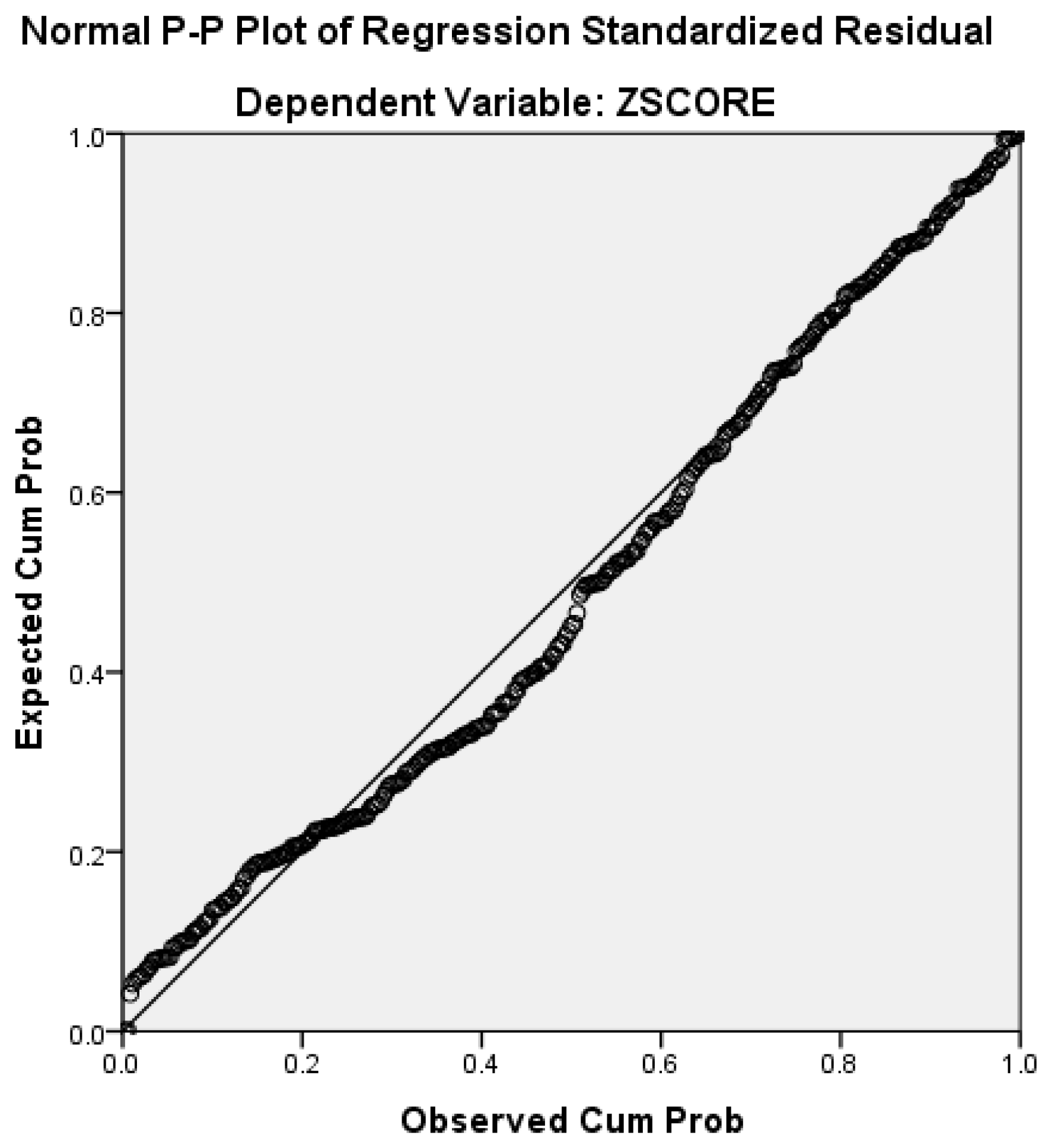
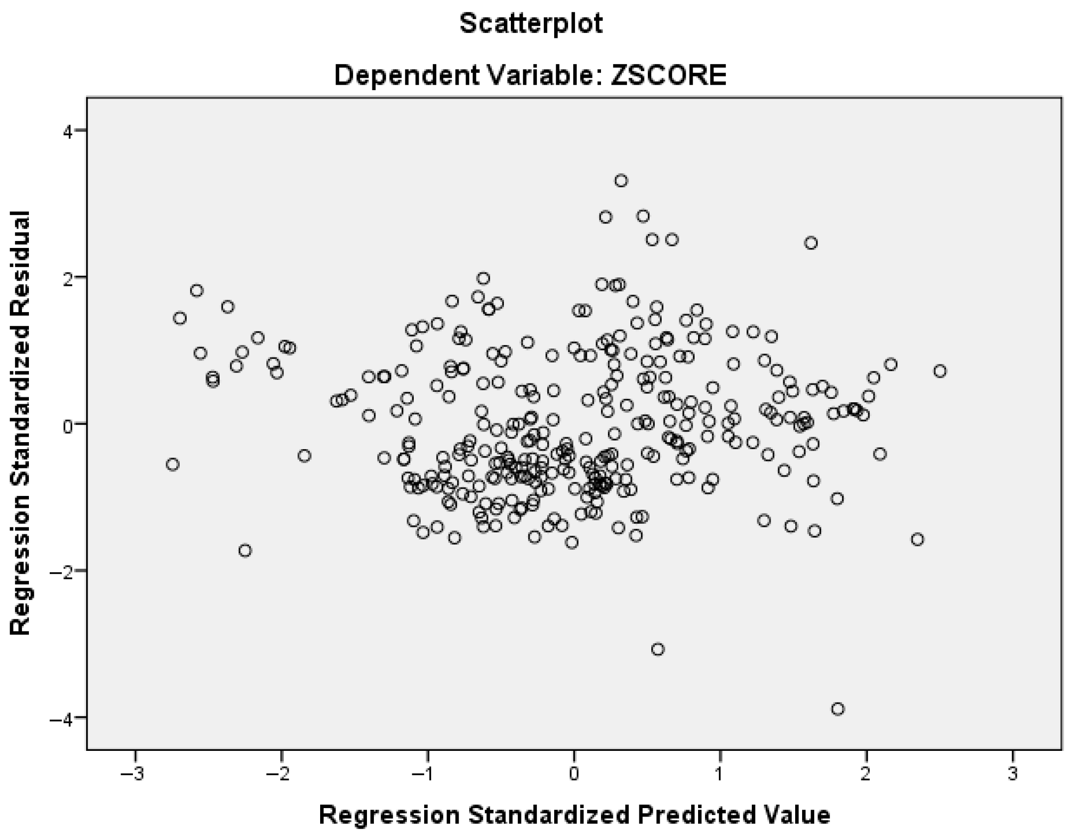
Building on the econometric diagnostics and variable validation, which achieved an adjusted $R^2$ of 0.860 and resolved autocorrelation via the lagged Z-score (Durbin–Watson ≈ 1.915), we now assess out-of-sample performance using machine learning classifiers. The evaluation uses the DISTRESS label derived from the Altman Z-score threshold (1.8) defined in the cleaning stage, ensuring consistency between the econometric specification and the classification target. To avoid leakage, all preprocessing fits on the training were split and applied to the held-out test set.

In the present study, the empirical dataset consists of a panel of firm-year observations (N = 315) across 21 firms from 2010 to 2024, and the primary objective of the machine learning analysis is to compare the relative performance of different algorithms rather than to simulate a real-time deployment at a specific historical cutoff.

For this reason, we initially adopted a stratified 80–20 split at the observation level, ensuring that the class distribution of financially distressed and non-distressed firms was preserved in both the training and test sets. This approach is commonly used in the financial distress literature when the focus is on algorithmic discrimination and robustness, rather than on point-in-time forecasting.

4.3.1. Data Preparation and Cleaning (Concise)

We compiled an unbalanced panel of 21 German manufacturing firms (2010–2024) with firm-level ratios (SIZE, ROA, ROE, PM, OPEFF, OPEFF2, LIQ, SLV, LEV, Growth, FinMat), macro-indicators (GDP growth, Interbank Rates, INF, UNEMP, EXR, IDEBT), and the continuous Altman Z-Score. Column labels were standardized and all numeric fields were coerced to numeric types; firm identifier (Name) and Years were retained only for indexing. Missing numeric values were median-imputed column-wise. To limit the impact of extreme observations while keeping all rows, PM, OPEFF2, and Growth were winsorized at the 1st and 99th percentiles. For classification, we constructed DISTRESS = 1 if Z-Score < 1.8, else 0; identifiers were excluded from the feature set. A reproducible workbook with CLEANED, Missing_Report, Winsorization_Report, and Data_Dictionary sheets documents every step.

4.3.2. Experimental Design (Data Split, Pipelines, Algorithms)

Objective. Build a classification model for firm–year financial distress using the cleaned panel and compare algorithm families under a consistent, leakage-aware validation protocol.

Data split and leakage control. We partition the data 80/20 into training and test sets with stratification on the DISTRESS label to preserve class balance. All preprocessing transformers (imputation, scaling) are fit on the training set only and then applied to the test set. Identifiers (Name) and Years are excluded from the feature matrix; ZSCORE is excluded when the target variable is DISTRESS.

Pipelines.

Linear/Kernel models (Logistic Regression, SVM-RBF): median imputation → z-score standardization (scale-sensitive).

Tree ensembles (Random Forest, Gradient Boosting): median imputation only (no scaling needed).

Class imbalance. We set class_weight = “balanced” for scale-sensitive and tree models to correct for any minority-class under-representation.

The machine learning algorithms considered in this study, along with their corresponding model families and hyperparameter settings, are summarized in

Table 7. Algorithms and settings (kept modest to avoid overfitting).

Model	Family	Key Settings
Logistic Regression	Linear baseline	L2 penalty, class_weight = balanced, max_iter = 500
SVM (RBF)	Kernel margin	C = 10, gamma = scale, probability output on, class_weight = balanced
Random Forest	Bagging ensemble	n_estimators = 300, max_features = √p, class_weight = balanced, fixed random_state
Gradient Boosting	Boosting ensemble	n_estimators = 300, learning_rate = 0.1, fixed random_state

.

Evaluation protocol. We report Accuracy, Precision, Recall, F1, and ROC–AUC on the held-out test set. Confusion matrices and ROC curves provide error structure and threshold-free discrimination. Unless noted otherwise, the classification threshold is 0.50. For transparency, SHAP analysis is applied to the Gradient Boosting model (fit on the train set; SHAP computed and summarized on the test set) to indicate global feature influence and directionality.

Robustness add-on. We repeat the stratified 80/20 split 10× with different seeds {42…51} and summarize mean ± sd ROC–AUC to demonstrate stability of conclusions. Although the dataset includes 21 manufacturing firms, the empirical analysis is conducted on a panel of firm–year observations (N = 315) spanning 2010–2024. Accordingly, the train–test split is applied at the observation level rather than the firm level. An 80/20 stratified split is therefore appropriate and yields sufficiently large training and testing subsets for robust out-of-sample evaluation.

4.3.3. Evaluation Metrics

We evaluate all models on the held-out test set using Accuracy, Precision (TP/(TP + FP)), Recall (TP/(TP + FN)), and F1 (the harmonic mean of Precision and Recall), together with ROC–AUC.

Confusion matrices at a default decision threshold of 0.50 summarize Type-I errors (FP: false alarms) and Type-II errors (FN: missed distress)—with the latter generally being more costly from a financial-risk management perspective. We report ROC curves to compare models independent of any single threshold: the curve traces the trade-off between True Positive Rate and False Positive Rate across all thresholds, and AUC is the probability that a randomly chosen distressed firm is ranked above a healthy one (a threshold-free measure of discrimination). This makes ROC–AUC the appropriate primary metric when the operational cutoff may vary by user (e.g., bank vs. regulator).

Because the operating cutoffs used by practitioners may differ (e.g., bank vs. regulator), we adopt ROC–AUC as our primary, threshold-free comparator, and we complement it with fixed-threshold summaries (Accuracy, Precision, Recall, F1) and confusion matrices at 0.50 to show the concrete error profile. This protocol connects the ranking quality (ROC–AUC) to operational consequences (FN vs. FP), aligning the metrics with the assessment objective stated in our design.

Main finding. Ensemble learners outperform the linear and kernel baselines. Gradient Boosting attains the strongest discrimination (highest AUC), closely followed by Random Forest.

Table 8. Test performance by algorithm.

Model	Accuracy	Precision	Recall	F1	ROC–AUC
Gradient Boosting	0.857	0.882	0.857	0.870	0.953
Random Forest	0.873	0.886	0.886	0.886	0.947
SVM (RBF)	0.841	0.838	0.886	0.861	0.924
Logistic Regression	0.794	0.789	0.857	0.822	0.845

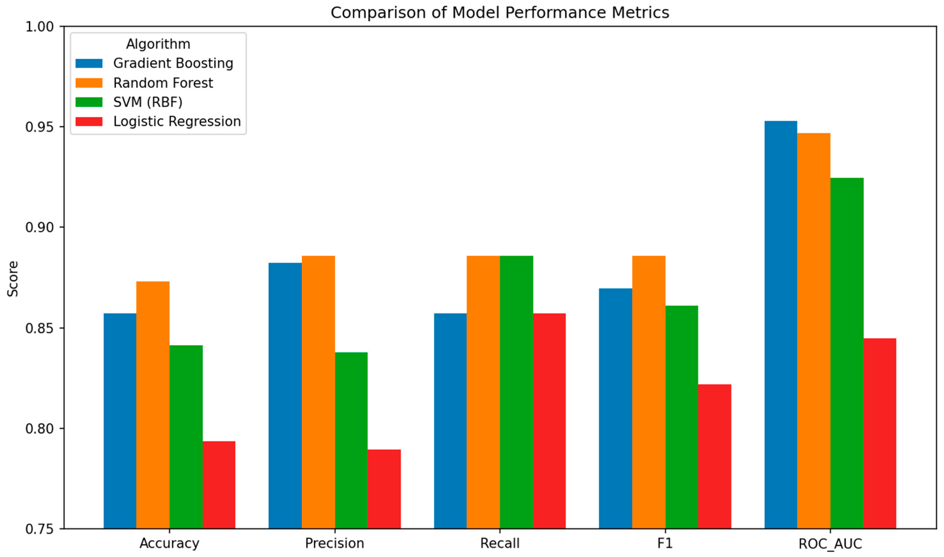
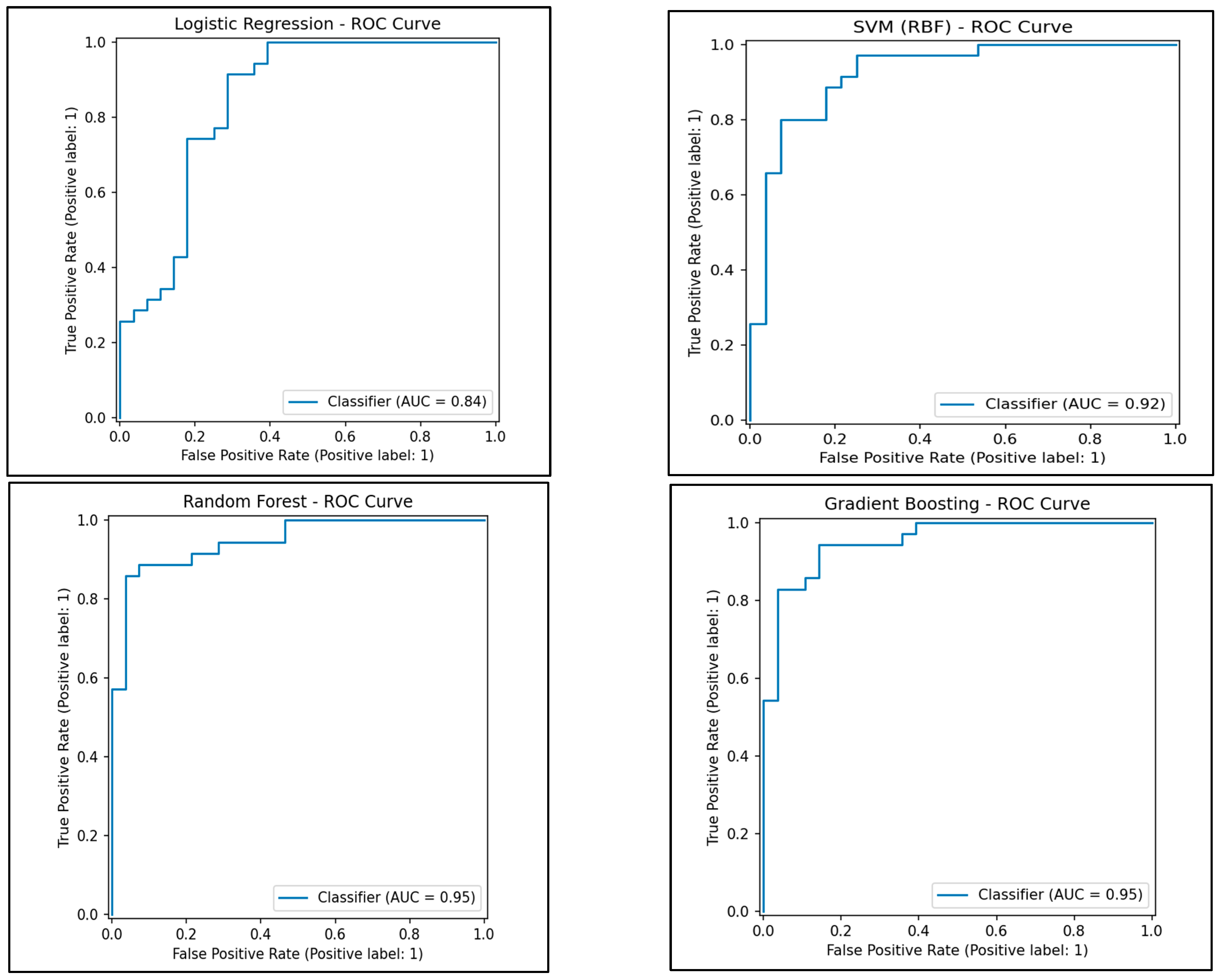
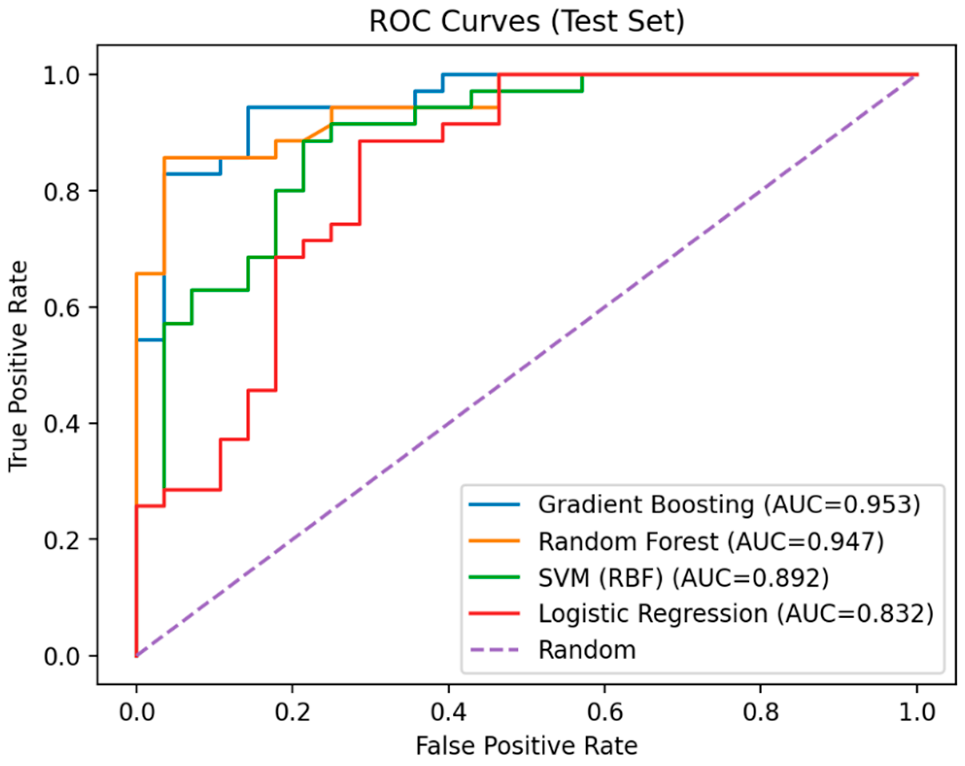
and Figure 7 summarize these differences across metrics, while the ROC curves in Figure 8 compare models across all thresholds without committing to a single cutoff.

Figure 7 contrasts Accuracy, Precision, Recall, F1, and ROC–AUC for the four classifiers on the held-out test set. Reporting this bundle of metrics is intentional: ROC–AUC captures threshold-free discrimination (how well a model ranks distressed above healthy firms across all cutoffs), while F1 summarizes the Precision–Recall trade-off at the default threshold (0.50). Accuracy is included for completeness but can be misleading when the costs of errors are asymmetric; in financial distress assessment, Recall (missed distress) and Precision (false alarms) matter more.

The figure shows a clear hierarchy. Gradient Boosting achieves the strongest overall discrimination (AUC ≈ 0.95) with competitive threshold performance (Precision/Recall/F1), indicating the best separation between distressed and healthy firms. Random Forest is a close second (AUC just below Gradient Boosting) and, in some metrics, matches or slightly exceeds it—together, these results highlight the advantage of tree-based ensembles in capturing non-linear interactions among financial ratios and macro indicators. SVM (RBF) performs solidly but trails the ensembles, and Logistic regression ranks last, consistent with the presence of non-linear effects that a linear boundary cannot fully model.

Practical implication. For practical implementation within a financial distress assessment framework, Gradient Boosting (or Random Forest) is the preferred base model. The operating threshold can then be tuned to the use case (e.g., favour higher Recall if missing a distressed firm is costlier than a false alert), but the AUC dominance in Figure 8 indicates that ensemble methods provide the most reliable foundation.

Figure 8 plots the Receiver Operating Characteristic (ROC) for all classifiers on the held-out test set, showing True Positive Rate versus False Positive Rate across all decision thresholds; the diagonal denotes random guessing, and curves nearer the top-left indicate stronger discrimination. The Area Under the Curve (AUC) provides a threshold-free summary of ranking quality. In our results, Gradient Boosting consistently dominates the ROC space, achieving the highest AUC (≈0.95), with Random Forest a close second; SVM (RBF) performs respectably but remains below the ensembles, while Logistic regression lies closest to the diagonal. Notably, in the low-FPR region—the operating zone when false alarms are costly—both ensemble models sustain comparatively high recall, reinforcing their suitability for practical financial distress assessment. (Models were fit on the training split only; ROC and AUC were computed exclusively on the unseen test data).

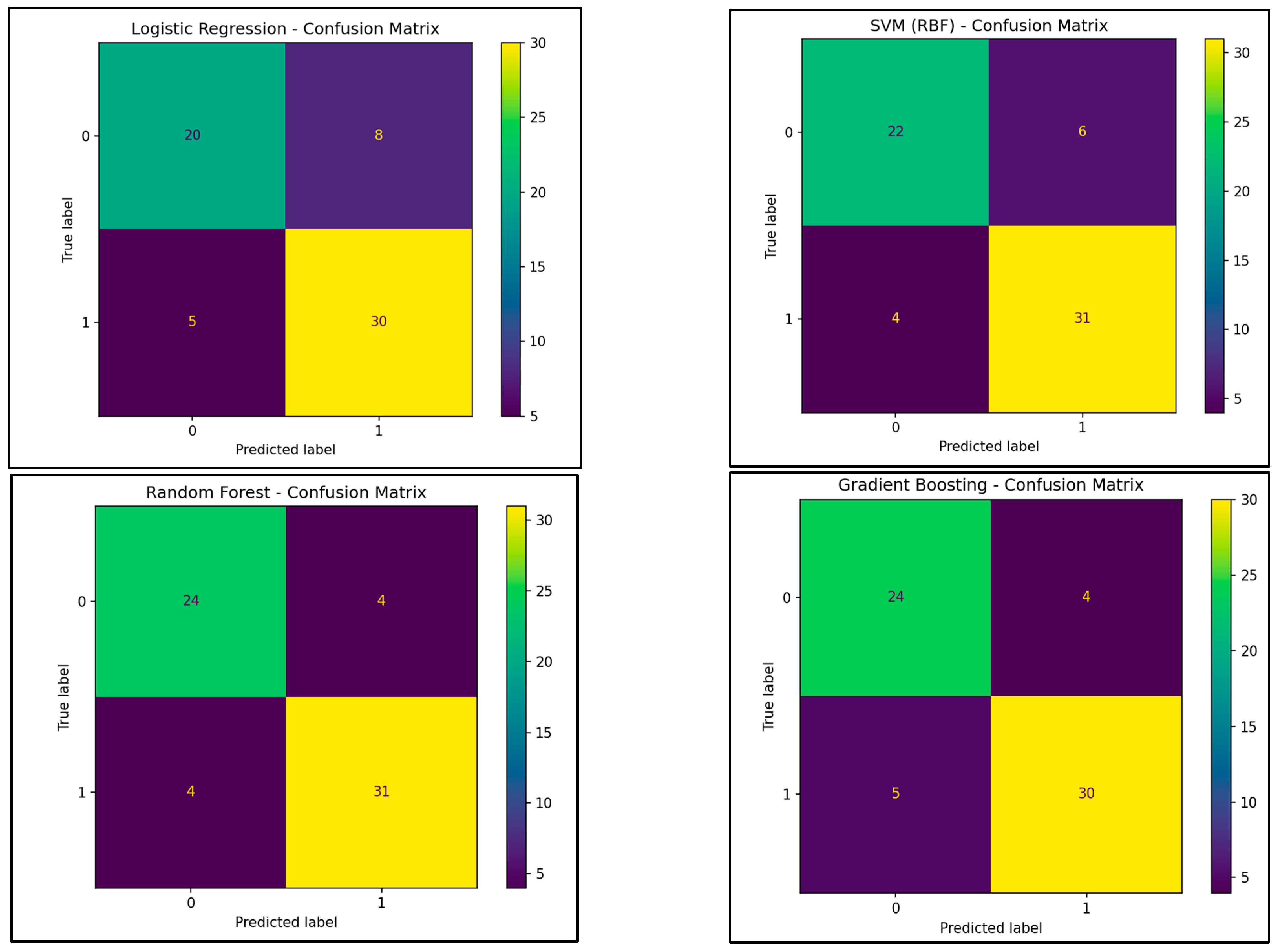
Figure 9 displays each classifier’s confusion matrix on the held-out test set at the default threshold (0.50), showing the distribution of true and false positives and negatives to reveal the error profile at an operational cutoff.

In our results, the ensemble models (Gradient Boosting and Random Forest) achieve fewer false negatives (missed distress) without materially increasing false positives (unnecessary alerts), consistent with their higher Recall and F1 in Table 8. Most residual errors cluster near the Altman Z boundary (~1.8–2.0), where firms are borderline and small shifts in ratios can flip the label—an economically plausible ambiguity. Practically, if minimizing missed distress is paramount, the decision threshold can be tuned below 0.50 (e.g., by maximizing Youden’s J or using a cost-based rule) to trade a modest rise in false alarms for a reduction in false negatives while retaining the ensembles’ superior discrimination.

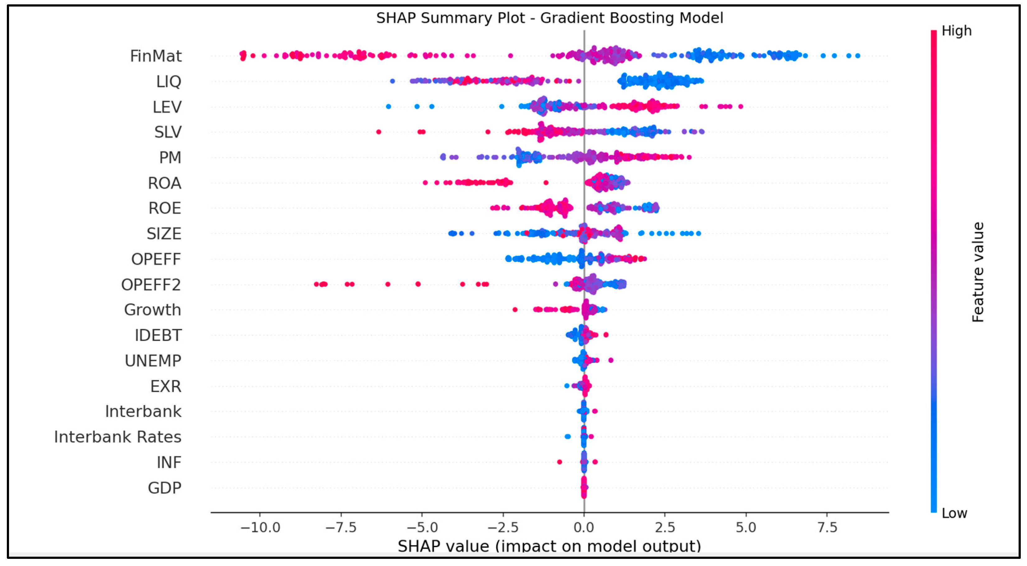
To explain why the best model performs better, we apply SHAP to the Gradient Boosting classifier (fit on the training set; SHAP computed and summarized on the test set). Therefore, SHAP values and permutation importance are interpretability tools that describe model-based contributions rather than statistical significance tests. The SHAP summary (Figure 10) ranks features by global impact and shows directionality.

Global insights. The SHAP summary plot (Figure 10) ranks features by mean absolute contribution and shows directionality (colour: high vs. low feature value).

• Stabilizers (negative SHAP): higher ROA, Liquidity (LIQ), and Financial Maturity (FinMat) reduce model-estimated distress.
• Risk drivers (positive SHAP): higher Leverage (LEV), Operating Inefficiency (OPEFF, OPEFF2), and (in some regimes) PM raise model-estimated distress.

These patterns are economically coherent and align with signs from the econometric analysis.

Figure 10, reports the SHapley Additive Explanations (SHAP) summary for the Gradient Boosting classifier, providing both a global feature ranking (by mean |SHAP|) and the direction of their contributions to the model-estimated distress score. Each dot represents a firm–year; colour encodes feature magnitude (red = high, blue = low), and horizontal spread reflects each feature’s contribution size. The plot shows that higher ROA, Liquidity (LIQ), and Financial Maturity (FinMat) are associated with negative SHAP values—lower model-estimated distress score—whereas higher Leverage (LEV), Operating Inefficiency (OPEFF/OPEFF2), and (in some regimes) Profit Margin (PM) contribute positively to distress risk. These patterns are economically coherent and mirror the signs from our econometric analysis, indicating that the ensemble model’s decisions align with financial intuition. (Model fitted on the training split; SHAP computed and summarized on the held-out test set to avoid leakage. SHAP explains model-based associations, not causal relationships.)

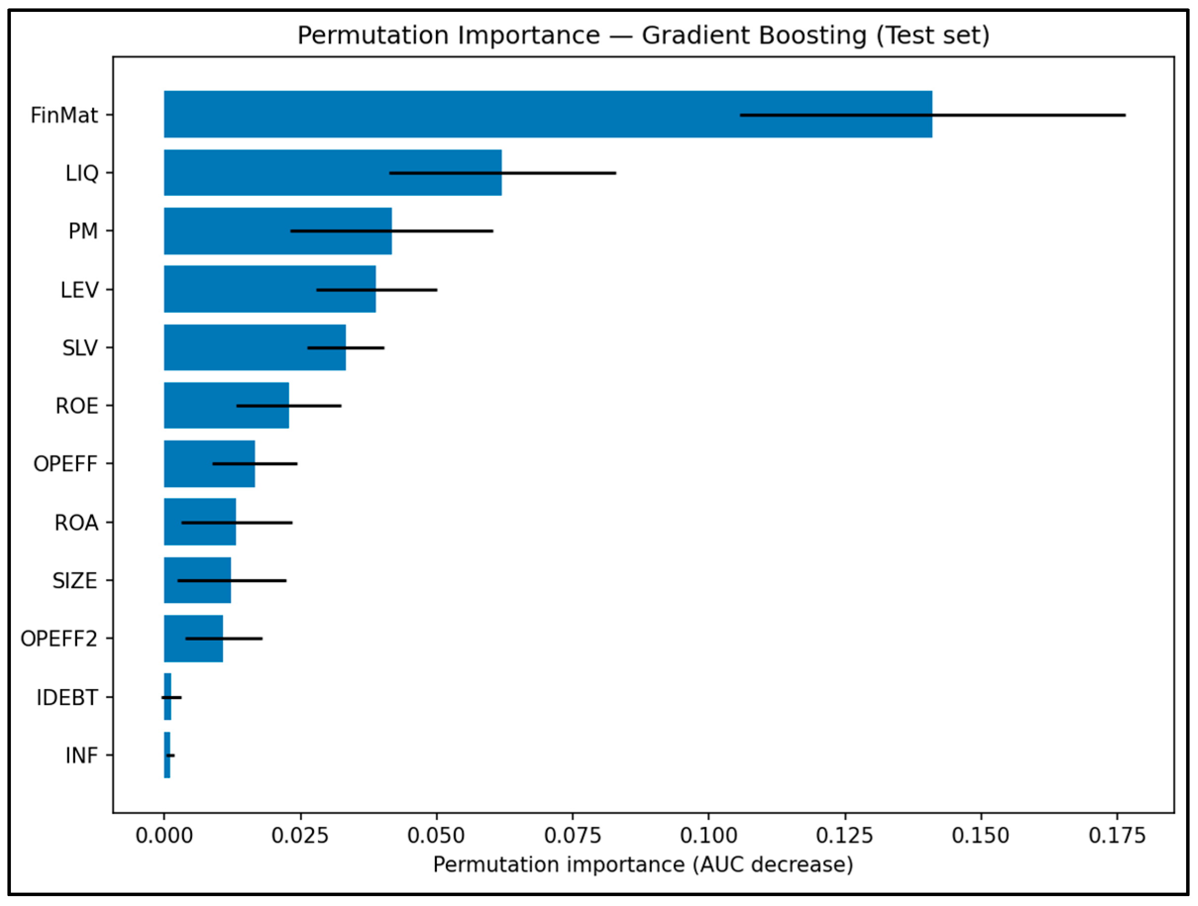
Figure 11 reports permutation importance for the Gradient Boosting model on the held-out test set (50 repeats). The ranking shows FinMat as the most influential factor by a wide margin, followed by LIQ and PM; LEV and SLV have moderate impacts, while ROE/ROA/SIZE contribute less once the leading variables are included. IDEBT and INF are near zero. This measure reflects each feature’s contribution to the model’s output magnitude, not its directional effect; directionality is provided by the SHAP results (higher LIQ/FinMat lowers risk; higher LEV/OPEFF raises risk).

To verify stability, we repeat the stratified 80/20 split 10 times with seeds {42…51} and re-estimate all models under the same pipelines. We report mean ± sd ROC–AUC per algorithm; dispersion is small, indicating conclusions do not hinge on a specific split.

All steps (cleaning, preprocessing, training, figures, SHAP, repeated runs) are scripted in Python version 3.13 (pandas, scikit-learn, matplotlib, shap).

Table 9. Comparison of model evaluation metrics.

Model	Specificity	Balanced Accuracy	MCC	ROC–AUC	Gini	PR–AUC	KS	Brier Score	Log Loss	ECE
Gradient Boosting	0.857	0.857	0.712	0.953	0.906	0.963	0.800	0.113	0.486	0.119
Random Forest	0.821	0.839	0.679	0.947	0.895	0.963	0.821	0.098	0.318	0.121
SVM (RBF)	0.786	0.836	0.678	0.892	0.784	0.906	0.671	0.139	0.430	0.093
Logistic Regression	0.714	0.786	0.580	0.832	0.663	0.843	0.600	0.167	0.506	0.156

reports additional standardized evaluation metrics recommended for financial distress and credit-risk modelling (Altman et al., 2023) [40]. These metrics complement traditional measures by accounting for class imbalance, probability calibration, and distributional separation between distressed and non-distressed firms. The results confirm that ensemble-based models, particularly Gradient Boosting and Random Forest, consistently outperform benchmark models across discrimination (ROC–AUC, Gini, KS), balanced performance (Balanced Accuracy, MCC), and probability accuracy (Brier Score, Log Loss, ECE).

As shown in Table 8 and Table 9 of Additional Metrics, the ensemble-based models achieve the highest specificity values, with Gradient Boosting (0.857) and Random Forest (0.821) outperforming SVM and Logistic regression. This indicates that ensemble models reduce false alarms while maintaining high recall, which supports the construction of a rigorous distress-assessment score.

Specificity values are derived from the confusion matrices reported in Figure 9, where ensemble models exhibit a lower number of false positives compared to benchmark models. Gradient Boosting achieves the highest MCC value (0.712), followed closely by Random Forest (0.679), indicating superior overall classification quality when accounting for true positives, true negatives, false positives, and false negatives simultaneously. In addition, the MCC results further reinforce the superiority of ensemble models under imbalanced financial distress conditions, consistent with Altman et al. (2023) [40].

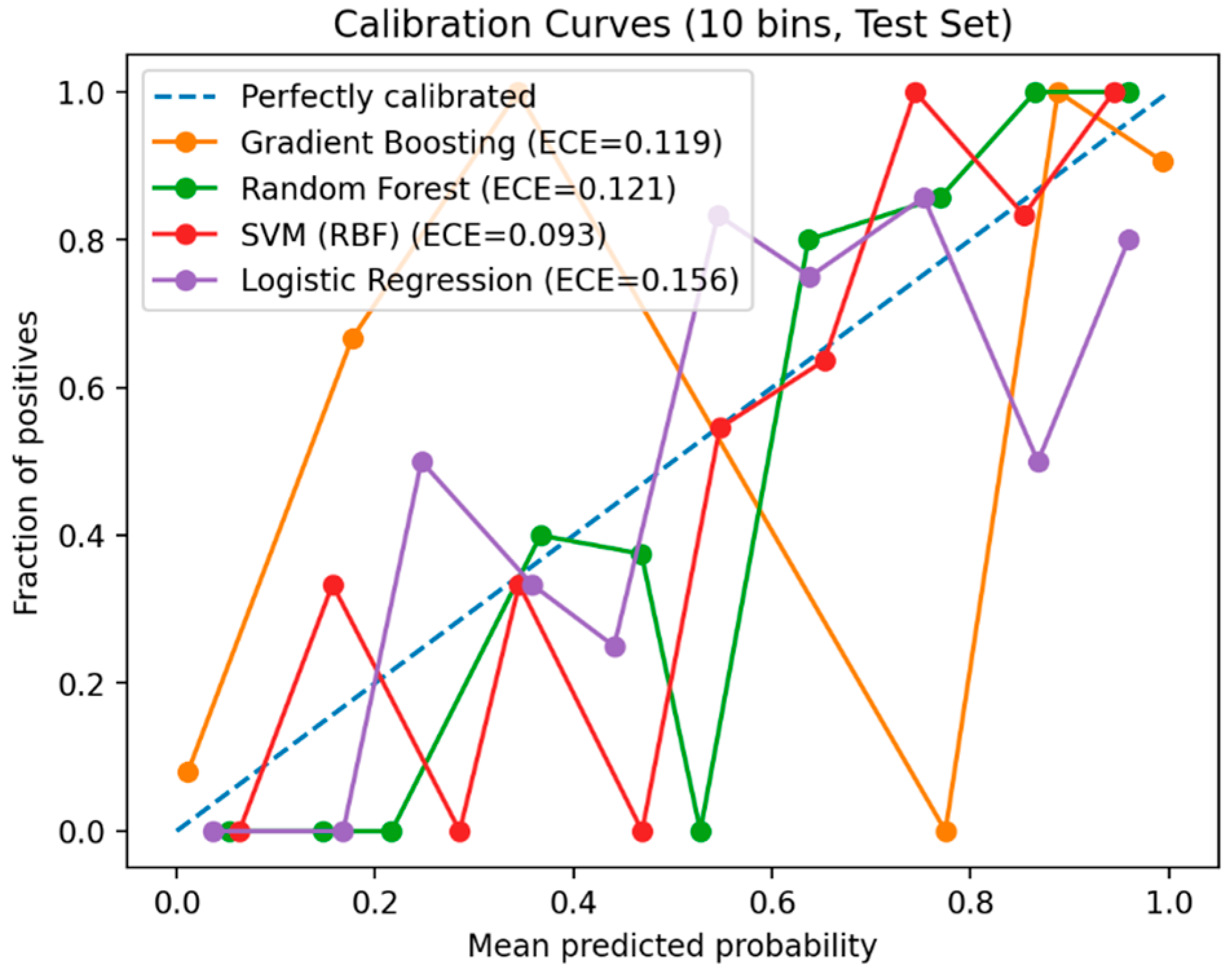
We have incorporated the Brier Score to evaluate the accuracy of the model-estimated probabilities rather than only class labels. As shown in Table 9, Random Forest (0.098) and Gradient Boosting (0.113) achieve substantially lower Brier scores than Logistic Regression (0.167), indicating better-calibrated and more reliable probability estimates. This is further visualized through the calibration analysis presented in Figure 12, where ensemble models closely follow the ideal diagonal calibration line.

As reported in Table 9, ensemble models yield lower log loss values, particularly Random Forest (0.318) and Gradient Boosting (0.486), compared to Logistic Regression (0.506). This indicates that ensemble methods assign higher confidence to well-estimated cases while penalizing incorrect probability estimates more effectively. The Gini coefficient, computed as $\mathrm{Gini}=2\times \mathrm{ROC}–\mathrm{AUC}-1$, has now been explicitly reported in Table 9.

Gradient Boosting achieves the highest Gini coefficient (0.906), followed by Random Forest (0.895), indicating excellent discriminatory power between distressed and non-distressed firms. These values are consistent with the ROC curves shown in Figure 13, where ensemble models dominate across all thresholds.

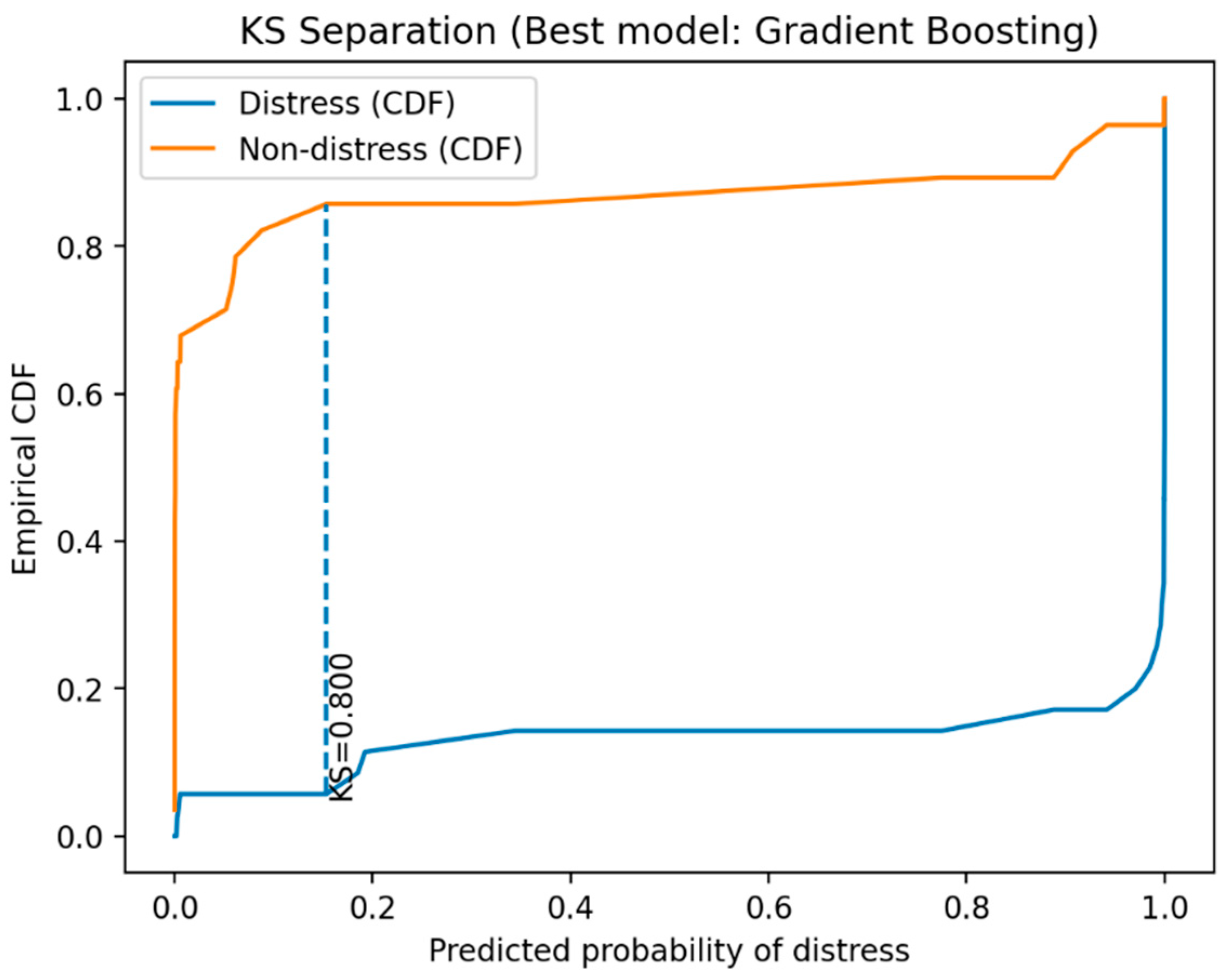
As reported in Table 9, Random Forest achieves the highest KS value (0.821), followed by Gradient Boosting (0.800), indicating strong separation between distressed and non-distressed probability distributions. This separation is visually illustrated in Figure 14, which plots the empirical cumulative distribution functions (CDFs) of both classes and highlights the maximum KS distance.

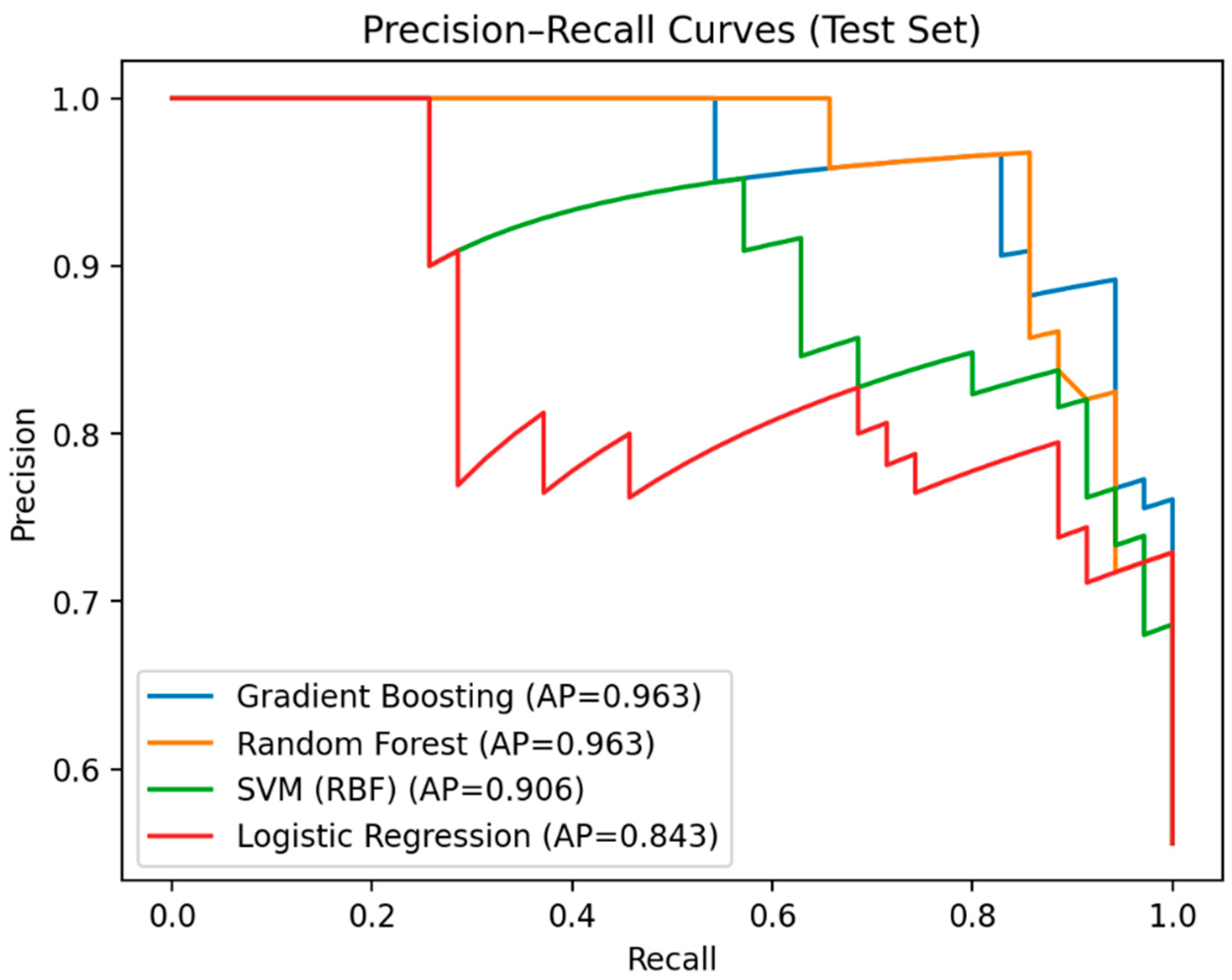
As shown in Table 9 and Figure 15, both Gradient Boosting (0.963) and Random Forest (0.963) achieve very high PR-AUC values, indicating strong performance in identifying distressed firms while controlling false positives. This confirms that ensemble models remain effective even under imbalance-sensitive evaluation.

We have added a comprehensive calibration analysis, including calibration curves and Expected Calibration Error (ECE). As illustrated in Figure 12, ensemble models demonstrate better alignment between their probability estimates and observed distress frequencies. Logistic Regression exhibits the highest ECE (0.156), while ensemble models show lower calibration error, indicating more reliable probability estimates. This analysis is particularly important for monitoring and risk-assessment systems where estimated probabilities provide more informative guidance than binary classification alone.

5. Discussion

The results of the econometric model found that the selected firm-specific and macroeconomic variables have a significant impact on financial distress measured by the original Altman Z-score, generating an adjusted R-square of 86% which supports the research hypotheses 1 and 2 that the firm-specific variables such as profitability, liquidity, leverage, and operating efficiency, as well as macroeconomic variables such as GDP, Inflation, and public debt, statistically affect the financial distress of the German manufacturing firms which are consistent with the studies of Charalambakis and Garrett (2019) [15], Khoja et al. (2019) [10] and Gregova et al. (2020) [16]. They suggest that increasing profitability and liquidity while enhancing operating efficiency by controlling costs relative to revenues, as well as reducing leverage, would improve the company’s financial health and mitigate the risk of bankruptcy. Furthermore, they contend that manufacturing firms are classified as cyclical businesses, which means they are more sensitive to the business cycle or to the changes in macroeconomic variables such as GDP and inflation that require careful and regular monitoring of the external economic environment to better manage for survival and growth. Moreover, based on the results of the ML, the Gradient Boosting and Random Forest models are outperforming the Logistic Regression and SVM, which is consistent with the studies of Huang and Yen (2019) [30], Malakauskas and Lakštutienė (2021) [19], Reimann (2024) [25], and Thacker and Saha (2025) [39] providing a scalable solution for continuous risk assessment within FinTech ecosystems. Therefore, the ML findings support hypothesis 3 that machine learning algorithms can accurately assess the financial distress levels of German manufacturing firms.

Furthermore, the results of feature importance are consistent with the findings of the employed econometrics which increases the robustness of the ML model of the study. Adityaningrum et al. (2024) [41] found that financial maturity has a significant negative impact, while Restianti and Agustina (2018) [42] and Abdelkader and Wahba (2024) [43] found it insignificant. In contrast, the results of this study showed that financial maturity has the highest feature importance in machine learning and has a positive significant impact on financial distress. This highlights the significance of incorporating financial maturity in the scoring model and suggests that a greater increase in retained earnings will improve the financial position of manufacturing businesses because higher retained earnings lower future financing costs and thus increase profitability, especially because leverage was found to be negatively significant, which is consistent with the findings of Chaudhary et al. (2023) [44], and illustrates how necessary it is to rely less on debt in compared to equity capital in order to reduce financial leverage, which raises the sensitivity of profit in relation to sales, particularly during the study period because businesses are facing significant volatility in sales and earnings.

6. Limitations

This study has several limitations that should be acknowledged. The sample is restricted to 21 large German manufacturing firms, which may limit the generalizability of the findings to small and medium-sized enterprises or to other European countries. Additionally, the research limits its study to financial variables, such as firm-specific and macroeconomic independent variables, excluding non-financial variables (such as governance practices and management quality) and event-based dummy variables (such as COVID-19), which may limit the model’s ability to capture a higher accuracy score.

Moreover, firms submit several yearly observations, which adds the possibility of temporal leakage within the firm. A firm-level grouping or time-based split was not used due to the short sample size (21 firms). This is recognized as a constraint in generalizing across enterprises. Additionally, although the panel structure provides 315 firm–year observations, the relatively small number of firms raises a potential risk of model overfitting, particularly when applying flexible machine learning algorithms. To mitigate this risk, the study employed several safeguards, including out-of-sample evaluation on a held-out test set, stratified data splitting, class weighting, conservative hyperparameter choices, and repeated train–test splits with multiple random seeds. The consistency of performance across repeated runs indicates that overfitting is limited, although it cannot be eliminated.

7. Conclusions and Recommendations

The study employed OLS regression to examine the relevance of specific firm-related and macroeconomic factors in determining financial distress in German manufacturing enterprises, achieving an R² of 86%. It then applied machine learning algorithms for assessing financial distress, with Gradient Boosting outperforming other methods, attaining an accuracy of 95.3%. As a result, the paper recommends that financial managers and CFOs of German manufacturing firms to use the developed scoring model to enhance the assessment and monitoring of financial distress, thereby reducing insolvency risks, and addressing declines in the Z-score.

Based on Nur et al. (2020) [33], Aydin et al. (2022) [1], and Elhoseny et al. (2025) [27], we recommend that future research use deep learning models by employing artificial neural networks (ANNs) to estimate financial distress, as they found that such models outperform traditional machine learning methods, which might yield higher accuracy scores than the machine learning approaches used in this study. Furthermore, the literature indicates that the Omega score developed by Altman et al. (2023) [40] shows that including non-financial variables improves the assessment of financial distress. Therefore, future work should consider adding non-financial and event-based dummy variables (COVID-19) to the existing model, potentially increasing the accuracy of the developed machine learning models. Additionally, for future research we strongly recommend that scholars adopt the same methodology but replace the original Z-score with updated versions or utilize the Expected Default Frequency or the Hazard Model of Default to conduct comparative studies, demonstrating which model is most accurate and reliable for evaluating financial distress.

Finally, the study recommends that policymakers or regulators of the manufacturing industry in Germany consider the research findings to pass new legislation that compels manufacturing enterprises to adapt to the new era of AI and Fintech by incorporating ML into their business models to enhance financial assessment and management performance in this highly dynamic environment. This would support the survival and growth of businesses, indirectly contributing to European economic growth. Additionally, the developed ML-based model could be utilized by treasury dashboards to provide automated alerts when manufacturing firms exhibit indicators associated with elevated financial distress. This model aligns with the architecture of modern FinTech risk-monitoring systems by delivering more accurate and reliable scoring outputs, thereby improving the assessment of financial difficulties.