
Article

Hardware Design Optimization of a Sparse Hyperdimensional Computing Accelerator for iEEG Seizure Detection †
MICAS, Department of Electrical Engineering, KU Leuven, 3000 Leuven, Belgium
*
Author to whom correspondence should be addressed.
This paper is an extended version of our paper published in 20th International Conference on PhD Research in Microelectronics and Electronics (PRIME 2025), Taormina, Italy, 21–24 September 2025: “iEEG Seizure Detection with a Sparse Hyperdimensional Computing Accelerator”.
Chips 2026, 5(2), 10; https://doi.org/10.3390/chips5020010
Submission received: 13 March 2026 / Revised: 17 April 2026 / Accepted: 20 April 2026 / Published: 23 April 2026
(This article belongs to the Special Issue New Research in Microelectronics and Electronics)

Abstract

Hyperdimensional computing (HDC) provides a highly efficient alternative to neural networks for intracranial electroencephalography (iEEG) seizure detection on edge devices with strict resource limits. While sparse HDC can significantly reduce energy use, current hardware fails to capitalize on this for two reasons. First, existing designs do not optimize the encoding architecture specifically for sparse execution, leaving potential energy savings on the table. Second, researchers often ignore the “area” problem, the large physical space high-dimensional vectors take up on a chip, which must be solved to make these devices small enough for practical edge use. This work presents a sparse HDC accelerator that bridges these gaps through three key contributions. First, we streamline the sparse encoding architecture to improve energy and area efficiency by integrating a compressed item memory (CompIM) and simplified spatial bundling. Second, to address the area bottleneck and enable true edge deployment, we systematically explore area trade-offs via sequentialization techniques, evaluating both channel folding (CF) and vector folding (VF). Third, we push efficiency even further by proposing an item-memory-free (IM-free) architecture. By replacing the baseline segmented shift binding with a standard shift binding scheme, and gracefully utilizing raw local binary pattern (LBP) codes directly as shift amounts, we completely bypass the CompIM for simultaneous area and energy savings. However, this optimization incurs a drop in detection accuracy; hence, we ultimately present two tailored configurations. First, our energy-optimized IM-free design achieves a 5.55× area and 3.08× energy improvement over the sparse HDC baseline, alongside 8.20× and 13.37× improvements over the dense baseline. Second, to prioritize clinical performance, our balanced streamlined design utilizes a channel folding factor (CFF) of 4 to preserve higher accuracy. This balanced approach achieves a 5.97× area and a 4.66× energy improvement over the dense baseline, with a 4× latency increase.

1. Introduction

As the demand for intelligence at the extreme edge grows, standard deep learning approaches often face prohibitive power and latency constraints. Hyperdimensional computing (HDC) has emerged as a compelling, low-energy alternative to traditional neural networks [1]. By computing with high-dimensional vectors (HVs) with typically 1000 to 10,000 dimensions, where each dimension is represented with one bit, HDC offers robustness against noise and typically requires significantly less training data, enabling efficient few-shot learning [1,2]. These characteristics make HDC especially suited for intracranial electroencephalography (iEEG) seizure detection: sensors can be trained from just a few recorded seizures, and the extended battery life of the implantable devices significantly enhances the patient experience [2,3]. The iEEG seizure detection with HDC algorithm is illustrated in Figure 1a.
While the majority of current research focuses on dense HDC [4], where HVs contain roughly equal numbers of zeros and ones, sparse HDC presents an opportunity to push energy efficiency even further. By utilizing vectors where the vast majority of elements are zero (e.g., a density of approximately 1%), sparse HDC can drastically reduce both area footprint and computational energy [5]. However, these benefits come at the cost of more complex operations, making it difficult to capture these efficiency gains in practical hardware implementations.
While a few prior works explore sparse HDC hardware [6,7,8,9], they fall short by failing to address two critical gaps. First, even though sparse HDC promises significant energy reductions, existing implementations fail to fully leverage these savings because they do not rigorously optimize the underlying HDC encoding architecture. This is illustrated in Table 1, where our foundational work [5] is able to push energy efficiency further than the state-of-the-art (SotA) sparse HDC accelerators [6,7,8,9]. Second, the existing literature critically overlooks the exploration of area trade-offs for sparse HDC, even though reducing the large silicon area inherent to working with high-dimensional vectors is paramount in making these devices viable for edge deployment [10]. The lack of research into area efficiency is highlighted in Table 1.
In this work, we present a sparse HDC accelerator for iEEG seizure detection application that bridges these gaps to practical efficiency through three key contributions, illustrated in Figure 1b:
(1)
Streamlined encoding architecture: To maximize efficiency in our sparse HDC baseline [5], we integrate compressed item memory (CompIM) and simplified spatial bundling. Embedding binding into the item memory (IM) eliminates one-hot decoding, while omitting the post-bundling thinning step further improves area and energy efficiency without compromising accuracy.
(2)
Enabling edge deployment through sequentialization: To address the second gap and the critical silicon area bottleneck, we systematically evaluate channel folding (CF) and vector folding (VF) sequentialization techniques. Demonstrating that CF minimizes structural overhead, we implement a dataflow with a channel folding factor (CFF) of 4, trading manageable latency and energy increase for area reductions, making the design truly suitable for edge deployment.
(3)
Item-memory-free (IM-free) architecture: To push energy and area efficiency to new heights, we replace the baseline segmented shift binding with a standard shift binding scheme. By directly mapping the incoming six-bit local binary pattern (LBP) features to control the barrel shifters, we completely bypass the CompIM. While this algorithmic–hardware trade-off yields unprecedented simultaneous area and energy savings, it results in a noticeable drop in detection accuracy. We carefully explore this trade-off.
Ultimately, to accommodate different clinical and hardware constraints, we present two final accelerator configurations. For extreme edge deployment, prioritizing energy and area efficiency, our IM-free architecture achieves an 8.2× area and 13.37× energy improvement over our dense HDC baseline. Conversely, to prioritize clinical performance and protect detection accuracy, we propose a balanced architecture that effectively trades off area and energy improvements against the dense HDC baseline. Incorporating CompIM, simplified spatial bundling, and a CFF of 4, this setup achieves 5.97× less area and 4.66× less energy than the dense baseline, accepting a 4× latency increase.
The remainder of this paper is organized as follows. Section 2 introduces the fundamentals of sparse HDC and the iEEG seizure detection algorithm. Section 3 explains our baseline sparse and dense HDC implementations which are used to quantify the gains of our optimized architectures. Section 4 outlines the main contributions of our paper: the streamlined encoder architecture, reducing the area through CF and VF, and how the shift binding enables an IM-free architecture. Finally, Section 5 evaluates our contributions on algorithmic and hardware level and thoroughly compares our work with the current SotA [5,6,7,8,9,12,13,14,15,16,17,18]. To support reproducibility and further research, our complete software and hardware code is open-source and can be found at https://github.com/KULeuven-MICAS/sparse_HDC_for_iEEG, accessed on 22 April 2026.

2. Background

2.1. HDC Fundamentals

HDC, also known as Vector Symbolic Architectures (VSAs), is a computational framework that represents information using high-dimensional distributed representations called HVs [1,4,19]. Typically consisting of 1000 to 10,000 dimensions, these vectors can be composed of binary, real, or complex numbers depending on the specific model used. HDC operates on the principle that in very high-dimensional spaces, any randomly chosen vectors are quasi-orthogonal to each other [1,19]. This mathematical phenomenon, known as the concentration of measure, allows the system to represent a vast number of nearly independent “symbols” as HVs, while also being able to combine multiple HVs together in one and still distinguish its constituent parts [1].
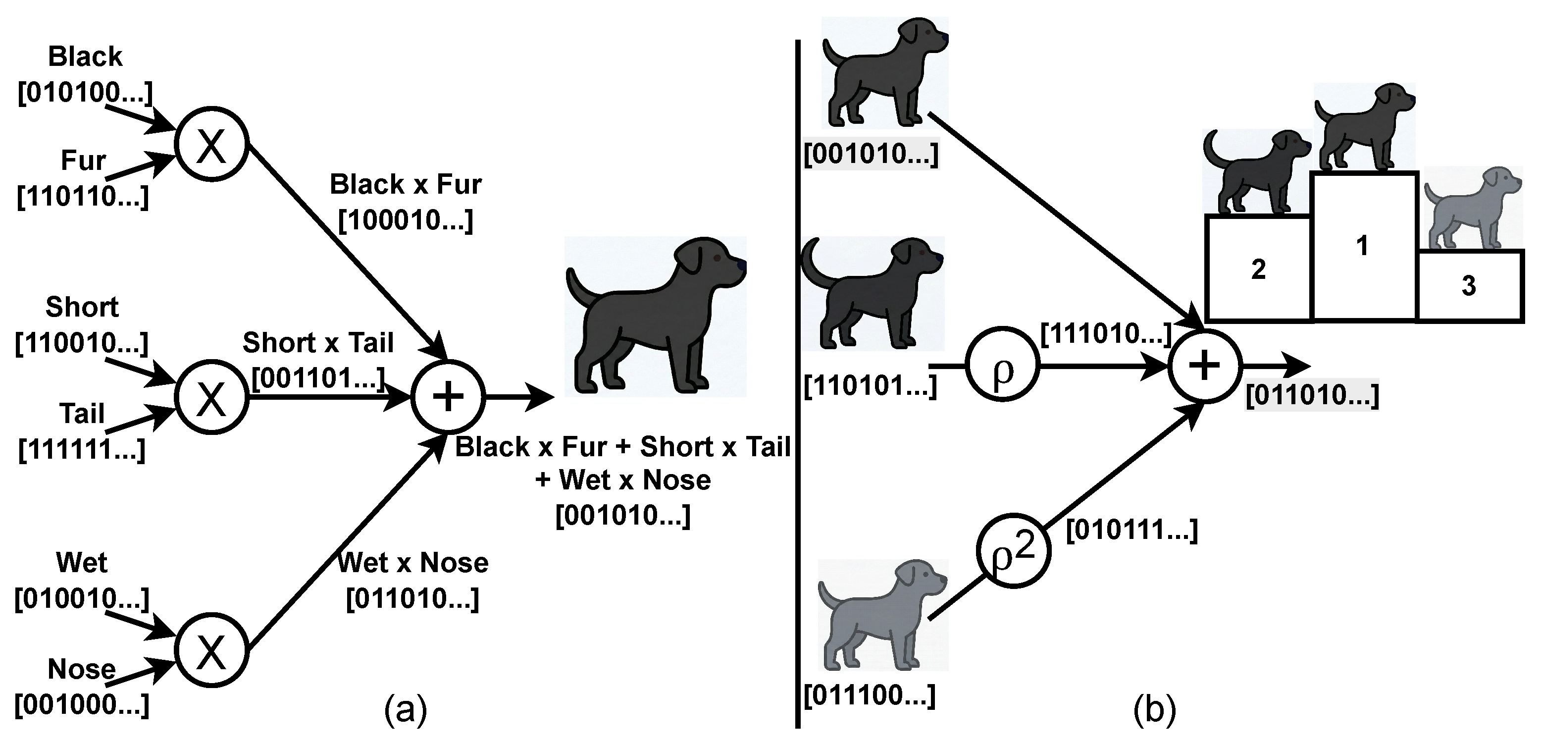
The HDC framework describes four fundamental operations to manipulate HVs: bundling (or superposition), binding, permuting, and a distance or similarity metric [1,19]. The output of the similarity metric scales between 0 and 1, where it is 0 if two HVs are perfectly orthogonal and 1 if two HVs are perfectly the same. The binding maps two HVs to one output HV, which is dissimilar to its inputs; this can be used to link two pieces of information together, as in Figure 2a, where the concepts “short” and “tail” are linked. The bundling combines a group of HVs into a resulting HV that is similar to each HV in the group. This can be used to combine features into one object represented by the bundled HV, as in Figure 2a, where the dog object is represented by the bundling of three of its aspects. The permutation takes one input HV and outputs an HV that is dissimilar. This is typically implemented by shifting the HV by a certain number of bits, as illustrated in Figure 2b, which can be used to link information regarding rank or position into a HV.
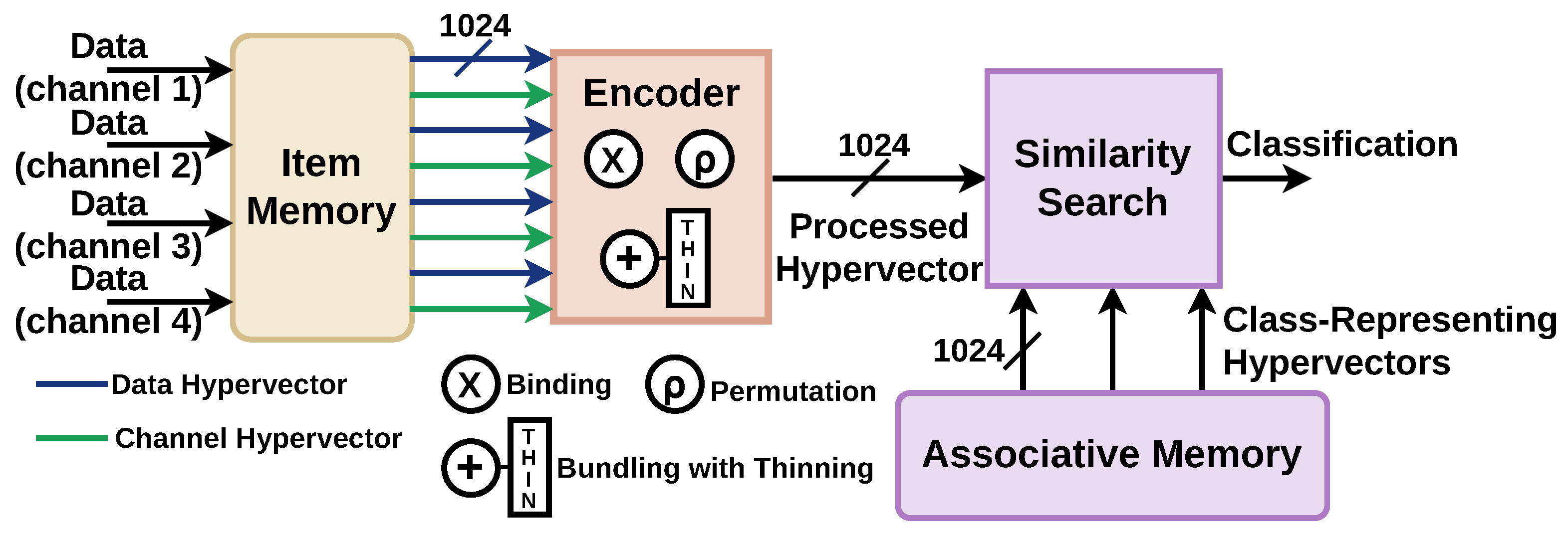
Figure 3 describes the structure of a general HDC algorithm [3,6,12,20,21]. Multiple data inputs go into the IM, where they are mapped to HVs corresponding to the data, depending on the application; other characteristics are also mapped to HVs, like the channel that the data came over; these HVs are then sent to the encoder.In the encoder, these HVs get combined into one processed HV through the use of binding, bundling, and permutation operations. How the HVs are encoded will depend on the application. This processed HV is then compared to class-representing HVs in the similarity search module, where the output classification corresponds to the class of the most similar class-representing HV. The class-representing HVs are stored in the associative memory (AM) and constructed in the training phase by feeding the same algorithm structure with training data and storing the processed HV in the associative memory, often with an extra bundling at the end of the encoder to bundle together multiple data points with the same class.

2.2. Sparse HDC Fundamentals

Sparse distributed binary HDC, in this paper referred to as sparse HDC, is a variant of the HDC framework, which means that the high-level algorithm structure can be maintained, while the specific HV representation and HV operations change [1,4,19]. Unlike dense HDC models, which use HVs with an equal distribution of 0- and 1-bits for the HV elements, sparse HDC HVs are mostly filled with 0s, and only 0.5 to 5% of elements are active, represented by 1 s.
The crucial advantage of sparse HDC is that sparsity leads to a large reduction in bit switches, which drastically lowers the dynamic energy. As seen in Figure 1c, the number of bit switches can be lowered by a factor of 25 for sparse HVs with a density of 1% compared to dense HVs. The disadvantage is that this sparsity needs to be managed, which complicates the HV operations. In particular, the binding needs to maintain the sparsity of its input HVs, and the bundling needs to control the sparsity throughout the encoder with thinning operations, as the superposition of HVs increases the density of the result [1,19].
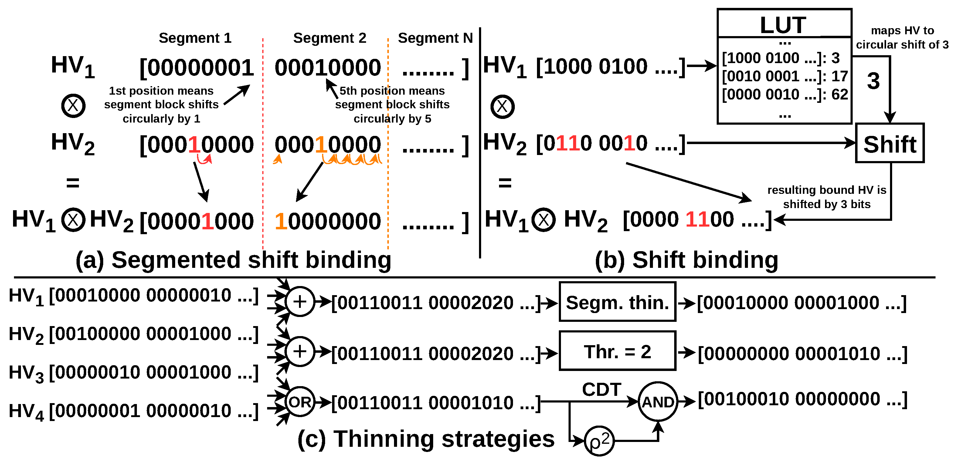
In sparse HDC, the similarity metric uses AND gates, as only the active bits carry information [1,19]. The binding can be implemented in three ways: segmented shift binding, shift binding, and context-dependent thinning (CDT) [1,19]. CDT is distinct from the other binding operations of HDC in that its output is similar to the inputs [22]; this property makes it unfit for the iEEG seizure detection algorithm as it relies on the binding to produce a dissimilar vector to its inputs [2]. Segmented shift binding and shift binding are suitable for the iEEG seizure detection algorithm and will be used in this paper. An example of segmented shift binding is shown in Figure 4a. Originally proposed by [23], this binding operation requires that the input HVs are split into segments of equal length, with each of these segments containing exactly one 1-bit. Then each segment of one of the input HVs is circularly shifted with the shift amount being equal to the position of the 1-bit in the corresponding segment of the other HV. Shift binding [1,19] is implemented by mapping one of the input HVs to a single value, which can be done by hashing [19] or a look-up table (LUT) [5], and shifting the other HV with this value, as illustrated in Figure 4. The permutation can still be used as before and is typically implemented with a shift as well.
Bundling requires combining multiple HVs in one representation. In the SotA [6,7,8,24,25], this process is implemented through a bitwise addition followed by a thinning operation. The thinning step is crucial for controlling the density of the output HV and preventing it from becoming completely filled with 1s, a common issue that arises when many HVs are bundled together. Preventing this saturation is essential because without it, the classification system breaks down. If an HV becomes saturated, it will incorrectly default to being most similar to whichever class-representing HV happens to have the most 1-bits, completely undermining proper, similarity-based classification.
Four ways to implement thinning have been proposed in the literature: (1) Segmented thinning [23], illustrated in Figure 4c, keeps the requirement of having exactly one 1-bit in each segment even after bundling; the elements are added together over the dimensions and the highest sum in each segment is kept as the 1-bit with the rest set to 0. In practice this becomes quite restrictive which can lead to low performance [7]. Other works [19,25] do not consider it and instead use maximum density thinning. (2) Maximum density thinning and (3) threshold thinning allow us to control the density after bundling with a hyperparameter [19]. This control makes them effective in many applications [5,7,8,19,24] but requires tuning the hyperparameter. Maximum density thinning is implemented by iteratively taking the largest sums after addition and setting these to 1-bits until a certain density (hyperparameter) is reached, with the remaining bits set to 0s.Threshold thinning compares the sums directly to a threshold value (hyperparameter) and sets the larger sums to 1-bits. Threshold thinning is often used in practice as a more hardware-friendly variant of maximum density thinning [5,6,7,8,20,26,27] and is illustrated in Figure 4c. Finally, (4) CDT can also be used as thinning after bundling [22]. The most popular version of CDT, additive CDT, is illustrated in Figure 4c.It takes the disjunction of the input HVs as input, which separates CDT from the other thinning implementations, as the bundling can be implemented by OR-gates instead of adders. Then the thinning is done by shifting the OR-gate output and AND-gating this with the unshifted OR-gate output; the result has a density that is the square of the density after disjunction [22]. This mechanism can be repeated to reduce the density further, and these outputs can be combined by disjunction to increase the density as well. This combination can be used to reach different densities. The disadvantage of this approach is that when many HVs are bundled together, the density after disjunction will approach 100 % , and because we can only reduce density through squaring the density, the thinning breaks down [19]. This makes it not suitable for applications where many HVs are bundled together, like the temporal encoder of the iEEG seizure detection algorithm [2]. This paper will use the threshold thinning because of its flexibility and hardware-friendly implementation.

2.3. iEEG Seizure Detection with HDC

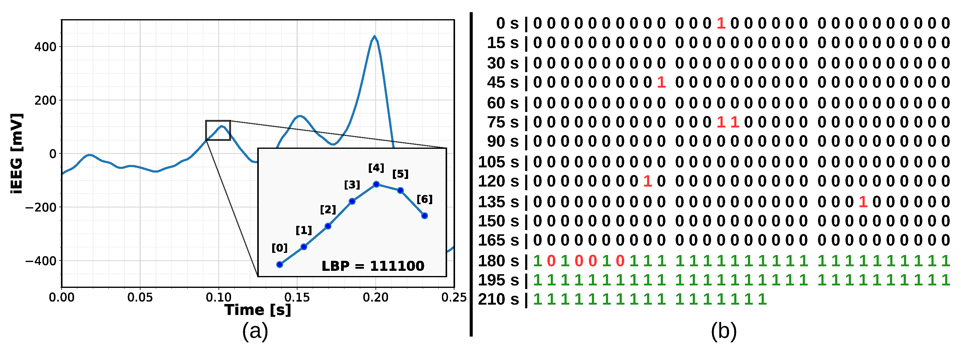
The iEEG seizure detection application aims to reliably identify the onset of epileptic seizures from brain activity, a crucial task for patients with drug-resistant epilepsy undergoing pre-surgical monitoring or utilizing implantable devices. Because iEEG recordings exhibit a massive asymmetry between interictal (normal) and ictal (seizure) states, detection systems require algorithms that can rapidly learn from a small number of seizure examples, referred to as one-shot or few-shot learning. Furthermore, because the seizure detection needs to be always on, it should operate with extreme energy efficiency to reduce the charging frequency for the patient. To meet these hardware constraints, the algorithm combines LBP codes with HDC. This algorithm is illustrated in Figure 5. For preprocessing, it extracts temporal features by comparing the amplitude of six consecutive samples. It assigns a 1 if the temporal difference between adjacent samples is positive, and a 0 otherwise. This generates a six-bit string, yielding 64 possible discrete symbols that capture local signal dynamics, illustrated in Figure 6a. These LBP symbols are sent to the IM, which assigns an orthogonal HV to every LBP code ( L 1 L 2 L 64 ) and electrode ( E 1 E 2 E n ). To encode spatial information, each LBP HV is bound to its corresponding electrode HV. These bound vectors are bundled across all electrodes to construct a single spatial record: S = [ E 1 × L i + E 2 × L i + + E n × L i ] . To capture the feature distribution over time, the algorithm bundles these S vectors over a 0.5 s moving window containing 256 time steps. Accumulating and binarizing these vectors via a threshold produces a temporal vector: H = [ S 1 + S 2 + + S 256 ] . For classification, the system relies on an AM filled with class-representing HVs, which were configured during the training phase. The AM contains two vectors representing the ictal and interictal states. During inference, the system assigns a classification label by computing the Hamming distance or similarity score between the newly generated H vector and the AM prototypes. To suppress false positives, postprocessing tracks the 10 most recent labels. A seizure is flagged only if the number of ictal labels exceeds a patient-specific threshold, typically set to 8–10. Figure 6b shows a typical example of the predictions, which illustrates that postprocessing is necessary, even though it increases the time before a seizure is flagged. The evaluation in [2] uses an anonymized dataset [28] of 16 patients. To simplify the performance metrics, this paper evaluates only the group of patients that achieve one-shot learning in the algorithm paper. Performance is measured by detection accuracy and delay. Minimizing delay is critical, as iEEG seizure onset often precedes clinical symptoms by more than 20 s; extending the delay can give patients valuable time to get to a safe situation or alert others. Cross-validation on a patient’s seizures is used for testing. Finally, we adapt this dense HDC algorithm to sparse HDC using segmented shift binding, threshold thinning for bundling, and an AND gate for computing the similarity score. In the HW implementations of this work, the number of electrodes is set to 64. This is taken as an average value, as for the patients of the dataset, this varies between 36 and 100. Furthermore, the HVs have 1024 dimensions ( D = 1024 ) and a density of 0.78125% ( p = 0.0078125 ), as the number of 1-bits is then also a power of two and close to 1%.

3. Baseline Accelerator Architecture

In this section, we detail the sparse and dense baseline accelerators we implemented for comparative analysis in our subsequent evaluations. The accelerator design is partitioned into five primary modules: the IM, the binding operations, spatial bundling, temporal bundling, and the similarity search with AM. The following subsections detail the hardware implementations of the baselines.

3.1. Sparse HDC Baseline

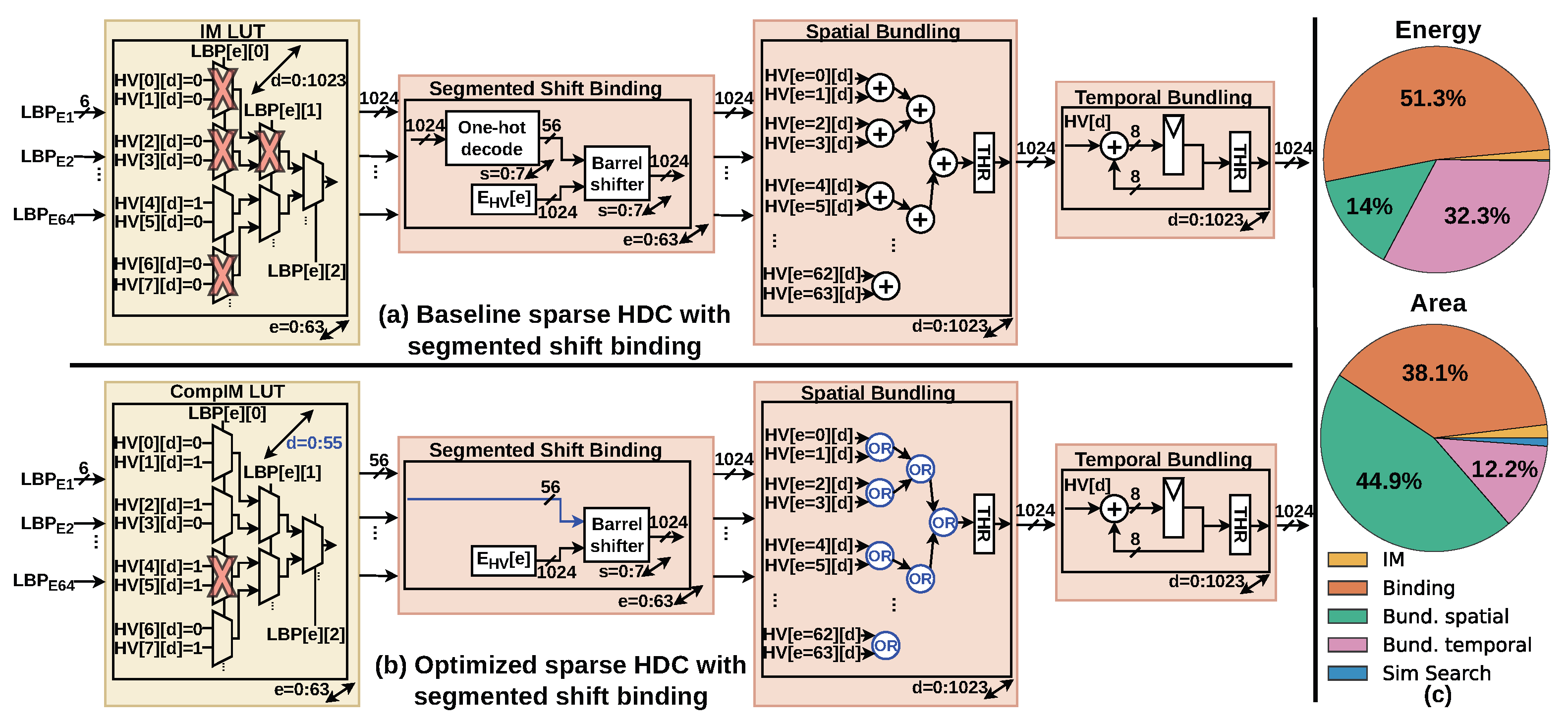
The IM maps a six-bit LBP code to one of 64 corresponding HVs using large LUTs. Because this mapping must occur for the values transmitted over each electrode, the architecture requires 64 parallel LUTs. Due to the high sparsity of the HVs, the synthesis tool can heavily optimize the internal LUT structure. As illustrated in Figure 7a, dimensions that are never activated can be hardwired to zero, while the remaining bits are only triggered under specific, limited conditions.
The binding architecture implements segmented shift binding (detailed in Section 2.2), which divides the two input HVs into parallel-processed segments. Given the vector parameters, the HV contains eight active bits ( D × p = 8 ), resulting in eight distinct segments. The operation identifies the position of the 1-bit within the first input HV’s segment and subsequently circularly shifts the corresponding segment of the second HV by that value. In hardware, this is realized using a one-hot decoder for the LBP HV segments, followed by a barrel shifter to rotate the electrode HV segments.
Spatial bundling is executed using an adder tree for each dimension. Each adder tree sums 64 1-bit inputs derived from the bound HVs. The resulting seven-bit sums are evaluated against a fixed threshold, and the binary comparator outputs form the spatially bundled HV. Following this, the temporal bundling module acts as an accumulator, storing the running sum in a large, eight-bits-per-dimension register.The input HV is added to this sum every clock cycle; after 256 cycles, the accumulated values are thresholded to produce the final binary HV.
Finally, the similarity search operates over two cycles and relies on a register to temporarily hold the processed HV. In the first cycle, a bitwise AND operation compares the processed HV with the interictal class-HV, and the outputs are summed across all dimensions to calculate and store a similarity score. During the second cycle, the similarity with the ictal class-HV is computed identically; the two similarity scores are then compared to assign the most probable class label. The hardware resource distribution of the sparse baseline implementation is plotted in Figure 7c, indicating that the primary bottlenecks for energy and area are the binding and spatial bundling modules, respectively. These inefficiencies serve as the primary targets for the optimizations introduced in Section 4.1.1 and Section 4.1.2.

3.2. Dense HDC Baseline

To provide a comprehensive evaluation, we also implemented a dense HDC baseline. This baseline mirrors the high-level structural framework of the sparse version but computes using dense HVs and dense HDC operations. Practically, this requires implementing the binding operation with bitwise XORs, setting the bundling threshold to exactly half the number of bundled HVs, and substituting the AND gates in the similarity search with XOR gates to compute the Hamming distance [1,2,19]. Because the original iEEG algorithmic framework [2] does not specify a hardware design, we constructed this implementation ourselves to benchmark against our sparse implementation. Consequently, to ensure a fair comparison, we integrated a well-established hardware optimization from the dense HDC literature, specifically, the bidirectional saturating counters proposed by [29] for the bundling operations.

4. Optimizations

4.1. Streamlined Encoding Architecture

This section details how the CompIM and simplified spatial bundling optimizations, proposed by our foundational work [5], tackle the major energy and area bottlenecks in the baseline architecture to create the streamlined encoding architecture in Figure 7b.

4.1.1. Compressed Item Memory (CompIM)

The first optimization leverages the extreme sparsity of the IM HVs to compress their bit-width and streamline the subsequent binding operation, which takes up 51.3% of the energy in the baseline accelerator. The baseline binding architecture is divided into two stages: a one-hot decoder that identifies the position of the single active bit within a large HV segment, followed by a barrel shifter. We can completely bypass this one-hot decoding logic by directly encoding and storing these active bit positions within the IM.
Given an HV dimensionality of D = 1024 , an HV density in the IM of p = 0.78125 % , and an HV segment length of D / ( p · D ) , this technique compresses the HVs to log 2 ( D / ( p · D ) ) · p · D = log 2 ( 1024 / ( 0.0078125 · 1024 ) ) · 0.0078125 · 1024 = 56 bits. While reducing the number of bits in this CompIM comes at the cost of making the LUTs dense, it does reduce the computational burden by allowing us to completely remove the one-hot decoders from the binding operation, as shown in Figure 7b. The overall hardware and resource effects of this optimization are discussed in Section 5.

4.1.2. Simplified Spatial Bundling

As indicated in the area breakdown of the baseline sparse HDC system in Figure 7c, the spatial bundling module is a major bottleneck, consuming 44.9% of the total area. To achieve a more cost-effective design, it is critical to reduce this hardware footprint. The baseline implementation was initially adapted from the dense HDC classifier for iEEG seizure detection [2] by transforming dense operations into their sparse equivalents [19]. In dense HDC, the bundling operation is always followed by a thinning step [2,12,20,21]. However, this thinning step is not strictly necessary for all stages in sparse HDC. In the context of our iEEG sparse HDC classifier, the spatial bundling stage combines 64 HVs. Because the input HVs have an extreme sparsity of 0.78%, the maximum possible density after spatial bundling, assuming absolutely no overlap of 1-bits, is exactly 50%.
Because the HV cannot become completely filled during this first bundling step, the thinning operation can be safely removed [5]. Eliminating the thinning requirement allows for a major hardware simplification: the large, area-intensive adder trees can be replaced entirely by simple OR trees.
As this architectural change modifies the output of the spatial bundling, its impact on the algorithmic detection performance is evaluated in Section 5.1. The resulting reductions in energy consumption and silicon area are detailed in Section 5.2.

4.2. Area Reduction Strategies: Channel and Vector Folding

Because HDC utilizes high-dimensional vectors, spatial parallelism inherently incurs a substantial silicon area footprint [29,30,31]. While previous sparse HDC accelerators have demonstrated promising energy efficiency improvements, SotA HDC works report significant area overheads even for relatively simple classification tasks [10]. Because the hardware footprint of the HDC accelerators scales linearly with the dimensionality of the HVs, this area bottleneck severely worsens for more complex applications requiring up to 10,000 dimensions. In the literature, HV lengths typically range from 512 to 10,000 dimensions [1,4], making this a critical scaling issue.
To alleviate this area bottleneck, we adapt two sequentialization techniques commonly used in dense HDC [32,33,34,35]: CF and VF. By reusing the same hardware blocks over multiple clock cycles, sequentialization trades increased latency and dynamic energy for a drastic reduction in required area. A comprehensive comparison of the hardware resource trade-offs between the CF and VF implementations is presented in Section 5.2.

4.2.1. Channel Folding

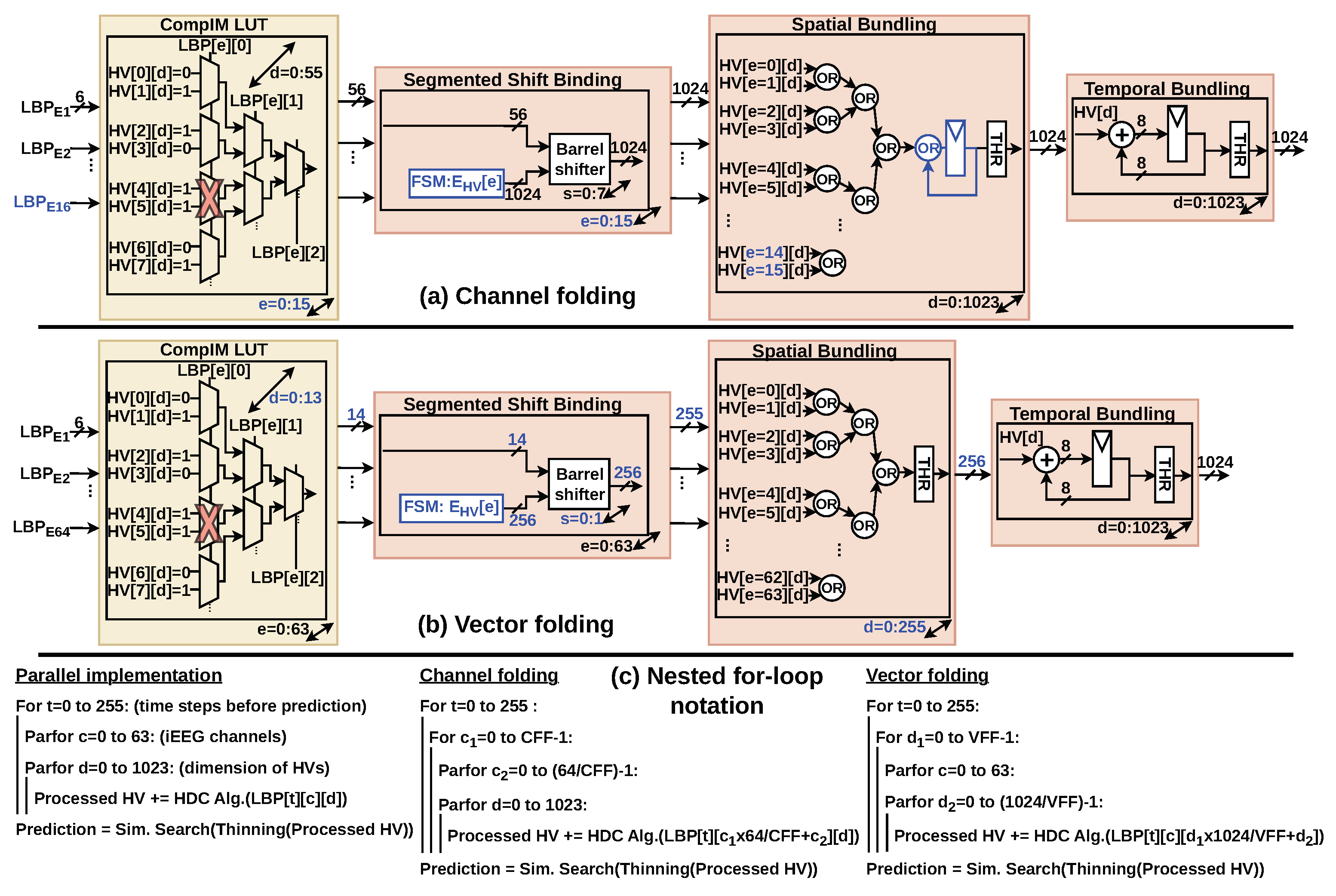
CF reduces the area footprint by processing only a subset of the input channels during each clock cycle. In the context of the iEEG seizure detection algorithm, which relies on 64 parallel channels, applying a CFF of 2 means that the algorithm processes 32 channels in the first clock cycle and the remaining 32 in the subsequent cycle. Consequently, this scales down the required number of LUTs in the CompIM, the total number of binding units, and the size of the OR-tree in the spatial bundling module by the CFF. The area consequences are illustrated in Figure 8a; the shift from parallel to sequential is illustrated with the nested for-loop notation [36] in Figure 8c.
However, CF introduces specific hardware overheads. It necessitates a finite-state machine (FSM) to supply the correct uncompressed electrode HVs sequentially to the binding module for each folded cycle. Furthermore, an extra accumulation register must be placed at the output of the spatial bundling OR-tree to temporarily hold and combine the bound HVs across cycles before they proceed to the temporal bundling module. Since the iEEG algorithm utilizes 64 channels, CF can theoretically achieve folding factors up to 64, provided the factor is a power of two.

4.2.2. Vector Folding

VF takes an alternative approach by processing only a fraction of the HV’s segments per clock cycle. In our baseline segmented shift binding, a 1024-dimensional HV with a 0.78% density is divided into exactly eight segments. With a vector folding factor (VFF) of 2, the algorithm processes four segments in the first cycle and the remaining four in the next cycle. This effectively halves the word length of the CompIM LUT output, shrinks the spatial bundling of OR-tree width, and decreases the number of binding units by the VFF, as illustrated in Figure 8b.
Unlike CF, VF eliminates the need for an extra intermediate accumulation register in the spatial bundling module. Nevertheless, it incurs an energy and logic penalty as extra hardware is still required to cycle through the parts of the electrode HVs, causing increased switching activity (and higher energy usage) within the binding module. Because there are eight segments in total for the chosen iEEG application parameters, the maximum possible VFF is limited to 8, whereas CF can theoretically scale up to a folding factor of 64. However, because CF structurally requires an extra accumulation register to temporarily hold and combine HVs across cycles, its inherent hardware penalty diminishes its overall efficiency.
The CF and VF implementations are evaluated in Section 5.2.

4.3. Item-Memory-Free Implementation with Shift Binding

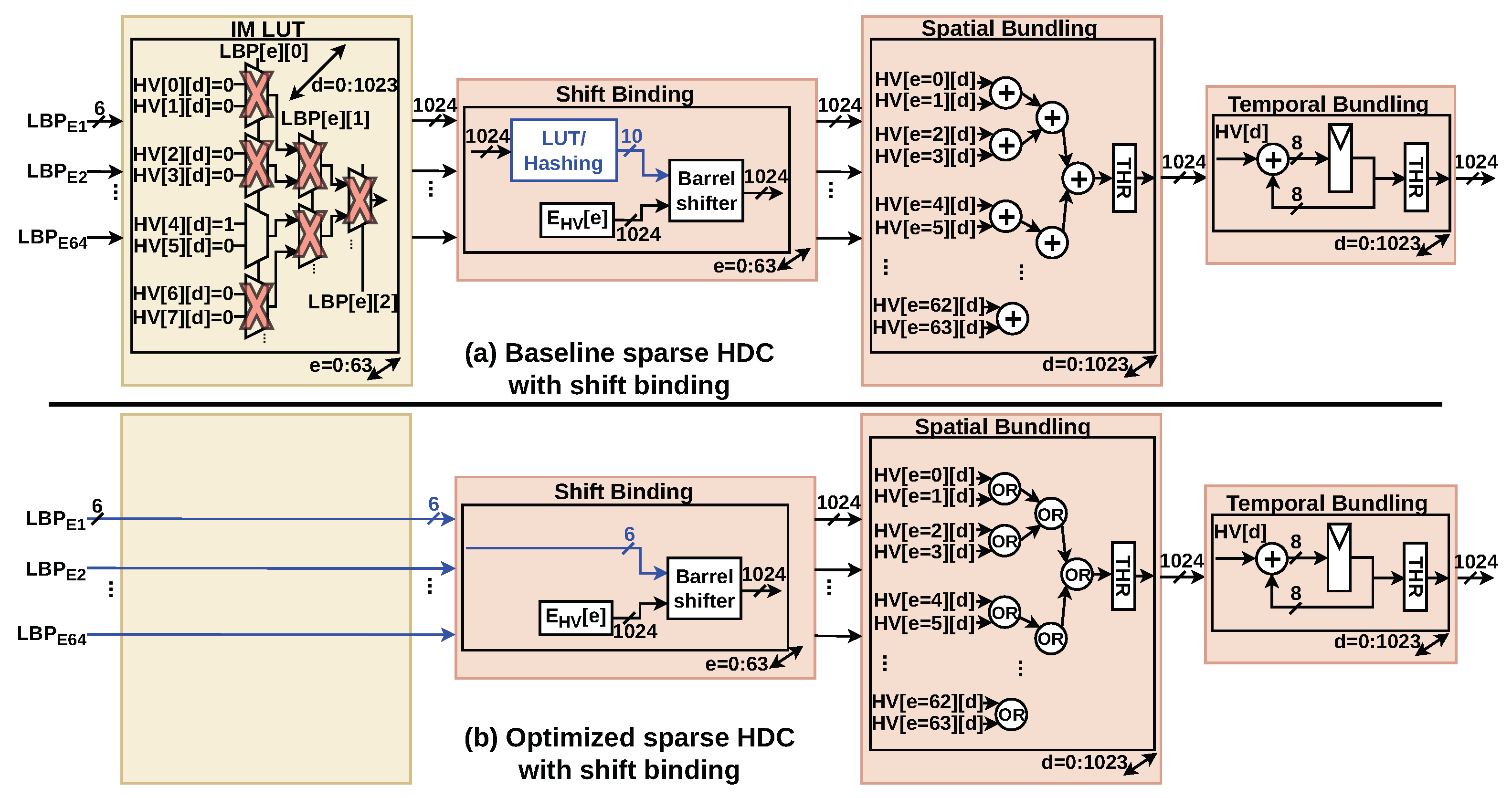
To enhance overall resource efficiency further, we investigate the transition from segmented shift binding to shift binding. The basic implementation of shift binding is described in the literature [19] as utilizing an LUT where each input HV is linked to a certain integer shift amount or a hashing function that converts the input HV into an integer. During the binding operation, one of the input HVs is mapped to this integer value, which then dictates the amount by which the second HV is circularly shifted. The HW architecture of the baseline with shift binding is shown in Figure 9a.

4.3.1. Bypassing the Item Memory

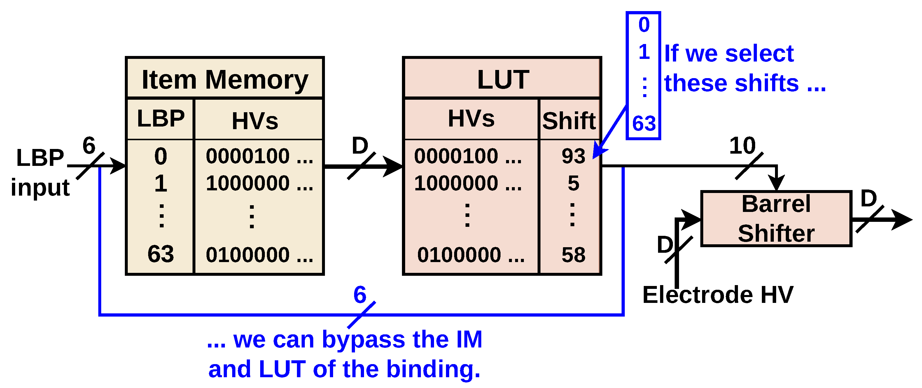
We illustrate the core concept of our IM-free architecture in Figure 10. Normally, an input LBP code is mapped to its corresponding HV in the IM. This D-dimensional HV is then subsequently mapped to a shift value corresponding to that HV. This shift value is then used to shift the electrode HV by that amount to complete the binding operation. In the literature [1,19], these shifts are initially randomly generated and placed in the LUT or are found through evaluating a hash function that takes the HV as input. These can be randomly generated as the point of the binding is to create a dissimilar HV from two input HVs, and shifting by a value of, e.g., 12 or 93, will give a dissimilar HV as output, which is also dissimilar to the other [1,7,19,22,37].
Because it does not matter which shift values are chosen for HDC to work, we could select these shifts to be equal to the LBP inputs. If we do this, the IM and the LUT of the binding do the exact opposite operation and can thus be canceled out or bypassed as in Figure 10. Consequently, the IM and LUT can be removed entirely, resulting in the architecture of Figure 9b.
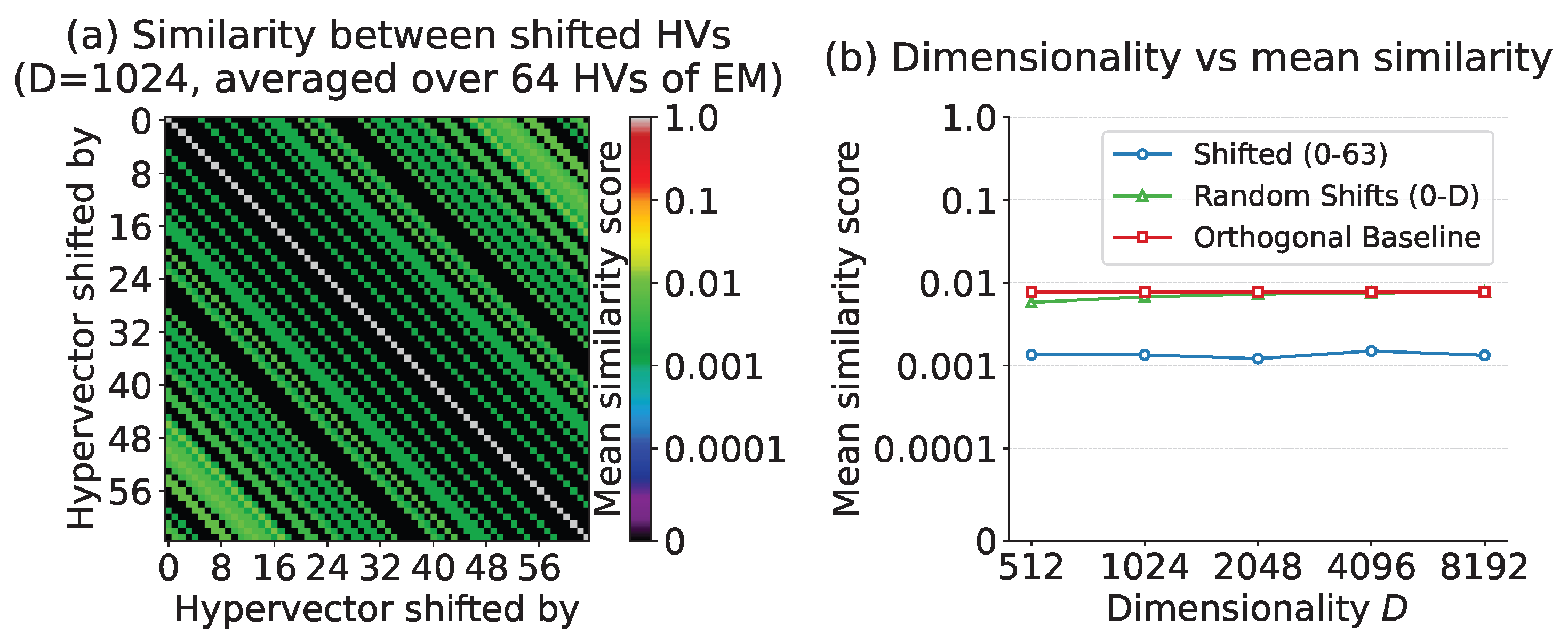
To show that limiting the shift values between 0 and 63 maintains sufficient quasi-orthogonality between HVs after binding, we provide the confusion matrix in Figure 11a. Here, the similarity score is plotted for HVs, which are shifted by values between 0 and 63, and the result is averaged over the 64 HVs of the EM. This shows that the amount of overlap is typically minimal, with the score being either 0 (no overlap at all, perfect orthogonality) or between 0.001 and 0.01, still 1000 to 100 times less similar than perfectly similar HVs. While this work keeps the dimensionality (D) at 1024 throughout, we would like to demonstrate the efficacy of the IM-free technique across a range of D from 512 to 8192. In Figure 11b, the mean similarity score is plotted over the range of D with the exception of the diagonal values, as these are always 1. This shows that D has little effect on the mean similarity score even when the shift values are limited between 0 and 63. This graph also shows that the similarity score is lower when the shifts are constrained between 0 and 63 than the provided baselines, meaning that the HVs are, on average, more orthogonal than when generating new random HVs or when selecting random shift values between 0 and D. However, for this application the more orthogonal HVs did not result in an improvement in algorithmic performance.
The algorithmic effects of the IM-free architecture on the iEEG seizure detection algorithm are studied in Section 5.1 and the effects on the hardware resources in Section 5.2.

4.3.2. Integration with Vector Folding

Integrating VF into the binding module initially appears more complex when employing standard shift binding. Unlike segmented shift binding, where individual segments are processed independently, standard shift binding requires a circular shift across the entire HV. Consequently, this introduces uncertainty regarding which bits must be shifted into the boundary of the vector at the start of a folded segment’s processing cycle, a complication that would inevitably demand additional hardware overhead to manage. Fortunately, SotA dense HDC architectures encounter a similar challenge during permutation operations. Recent studies [38,39] have explored permutation implementations within vector-folded architectures, demonstrating that individual chunks of the HV can be shifted independently without causing a degradation in overall classification accuracy. By adapting this insight to our design, the barrel shifter within the shift binding module is sized to match the dimension of a single vector-folded HV chunk. Each chunk is then circularly shifted by the identical LBP value, effectively integrating the segmented shift binding implementation with VF. CF can be implemented as described in Section 4.2.1.

5. Experimental Results

This section evaluates our proposed sparse HDC architectures at both the algorithmic and hardware levels. First, we assess the impact of our hardware–algorithm co-design on the iEEG seizure detection application. Subsequently, we provide a detailed hardware resource breakdown to quantify the area and energy improvements achieved by our optimizations, including the streamlined encoding, VF strategies, and the IM-free architecture. Finally, we benchmark our most efficient configurations against current SotA implementations.
All hardware experimental results are obtained from synthesis with Synopsys Design Compiler (U-2022.12-SP2) in TSMC 16 nm FinFET technology (TSMC, Hsinchu, Taiwan). The energy analysis is conducted using Synopsys PrimeTime (U-2022.12-SP2) with switching activity annotations. We also used clock-gating in synthesis; this setting results in minor changes compared to the results from [5]. For the algorithmic evaluation, we utilize the one-shot learning subset of the iEEG seizure detection dataset from [2,28]. To support reproducibility and further research, our complete software and hardware code is open-source and can be found at https://github.com/KULeuven-MICAS/sparse_HDC_for_iEEG (accessed on 10 April 2026).

5.1. Assessment of Algorithmic Performance

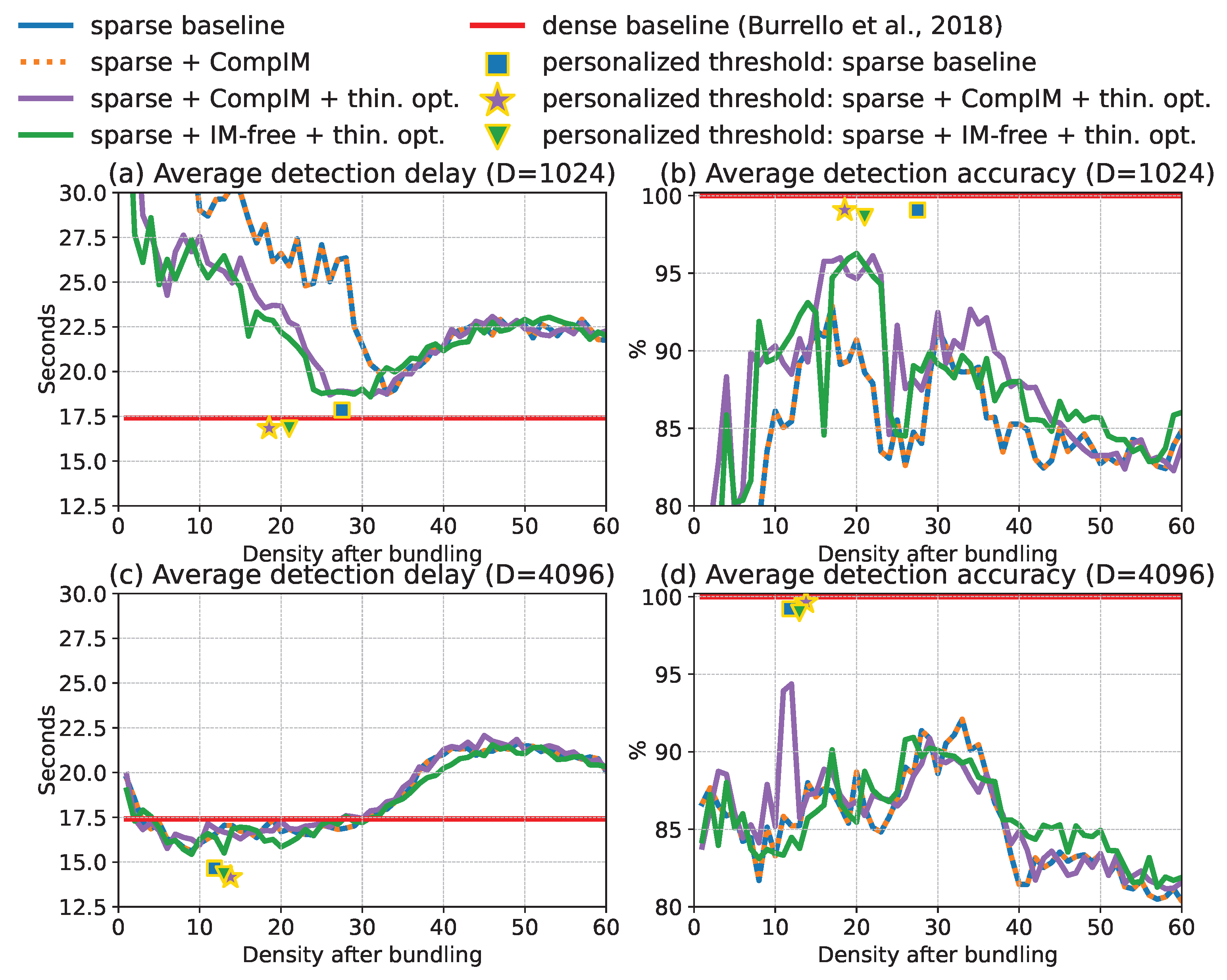
We evaluate our sparse HDC implementations at the algorithmic level and compare them against the dense HDC baseline. Figure 12 illustrates the results across our two primary metrics: average detection delay and average detection accuracy. The detection delay measures the time elapsed between the electrographic seizure onset and the algorithm’s alert. Because this electrographic onset often precedes clinical symptoms by more than 20 s, minimizing the detection delay is critical [2]; it maximizes the warning window the patient has to prepare before physical symptoms begin.
To thoroughly evaluate the sparse HDC implementations, we vary the threshold of the temporal bundling operation to control the HV density after thinning. The lines in Figure 12 show the average detection delay and accuracy when this threshold hyperparameter is kept constant across all patients. Because the CompIM is purely a hardware-level optimization, its algorithmic evaluation is identical to that of the naive sparse baseline. When incorporating the architectural changes, our results demonstrate that both the “CompIM + simplified spatial bundling” and the “IM-free + simplified spatial bundling” approaches perform better than, or at least equal to, the standard sparse baseline across the evaluated density range. We can safely simplify spatial bundling, even if it discards some data, as the chance of an overlapping 1-bit after the spatial bundling is very low compared to the temporal bundling ( P o v e r l a p = p 2 × 64 = 0.00390625 ).
While applying a universal threshold provides a general performance overview, in a practical clinical setting, the hyperparameter is tuned individually for each patient. To reflect this, the symbols in Figure 12 depict the maximum achievable performance, illustrating the average detection delay and accuracy when every patient is assigned a personalized, optimal threshold. Under these conditions, the streamlined sparse HDC architecture achieves a faster average detection delay than the dense HDC baseline (16.8 s for D = 1024 and 14.16 s for D = 4096 versus 17.4 s). However, this improvement comes at the cost of a slight drop in detection accuracy, decreasing from the baseline’s 100% to 99.1% for D = 1024 and 99.7% for D = 4096 . Furthermore, when comparing the optimized sparse architectures directly, the IM-free approach yields a slightly lower detection accuracy (98.6% for D = 1024 and 99.0% for D = 4096 ) than the streamlined approach. Because of these observed drops in accuracy, both the streamlined and IM-free architectures are explored further in the following sections.
While these detection accuracy drops do show a reduction in algorithmic performance compared to dense HDC, they do not necessarily mean that sparse HDC will always perform worse in practice for this application. As [2] shows, there are other techniques to increase the algorithmic performance, such as moving from one-shot learning to few-shot learning or tuning the postprocessing parameters.

5.2. Hardware Resource Breakdown and Comparison

5.2.1. Maximizing Efficiency Through Streamlined and IM-Free Architectures

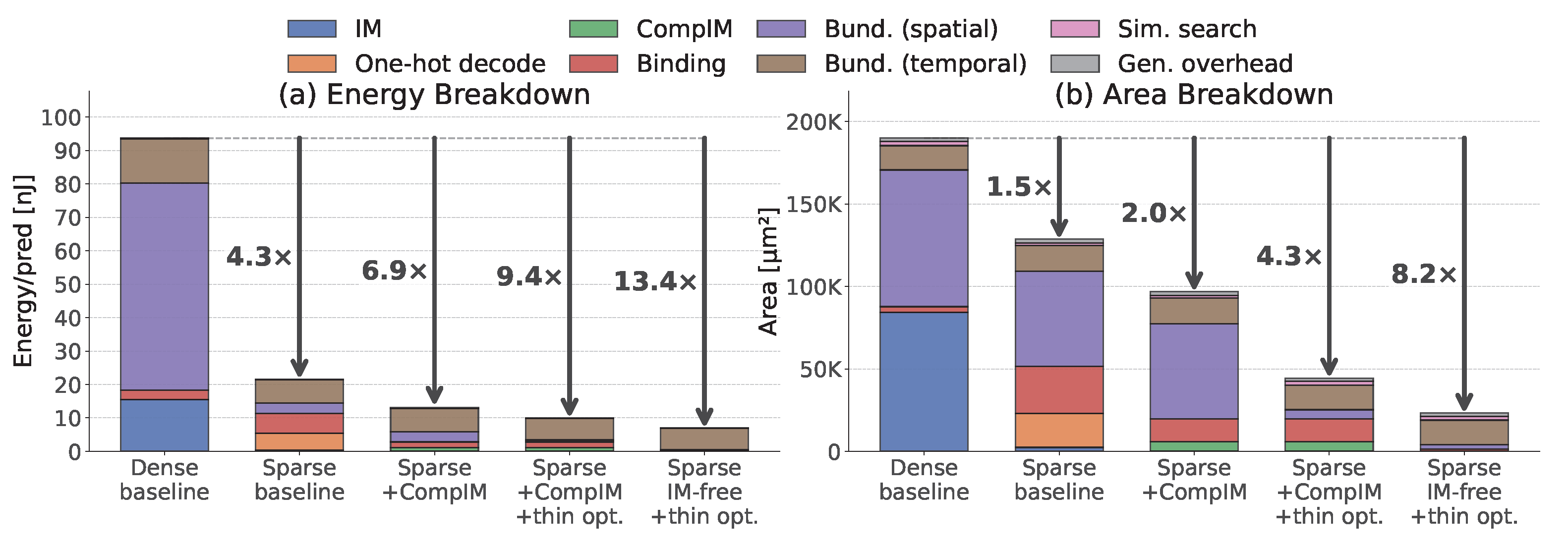
To fully understand the hardware impact of our proposed optimizations, Figure 13 visualizes a step-by-step breakdown of the area and energy footprint across different HDC architectures. The initial transition from the dense HDC baseline to the naive sparse HDC baseline yields a substantial reduction in overall energy consumption. However, this shift alters the hardware distribution, moving the primary system bottlenecks directly into the binding and spatial bundling modules.
As we apply successive layers of optimization, the structural benefits become highly apparent. First, integrating the CompIM significantly shrinks the binding overhead. By merging the IM and eliminating the power-hungry one-hot decoding logic, we drastically reduce the computational burden. Building on this, the simplified spatial bundling removes the thinning operation entirely. Because the extreme sparsity of the input guarantees the HVs will not saturate during this first step, we can safely replace the large, area-intensive adder trees with simple OR-trees. Together, these modifications result in a 2.16× energy improvement and a 2.89× area reduction over the sparse baseline.
The rightmost columns of the breakdown illustrate the ultimate impact of our IM-free approach utilizing standard shift binding. By mapping the incoming LBP features directly to control the barrel shifters, we are able to bypass the IM completely. This architectural leap drives both area and energy down to their absolute lowest points, achieving a total 3.08× energy and 5.55× area improvement over the sparse baseline. Notably, in this highly optimized IM-free configuration, the remaining energy footprint is nearly entirely dominated by the temporal bundling module.

5.2.2. Balancing Area and Energy: A Comparative Analysis of Folding Strategies

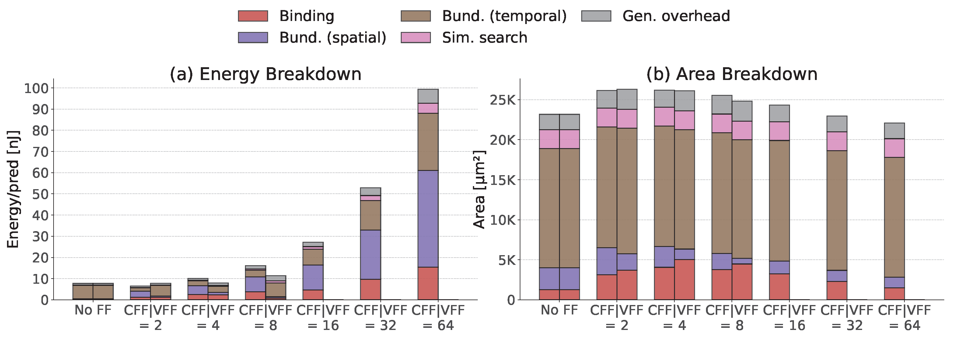
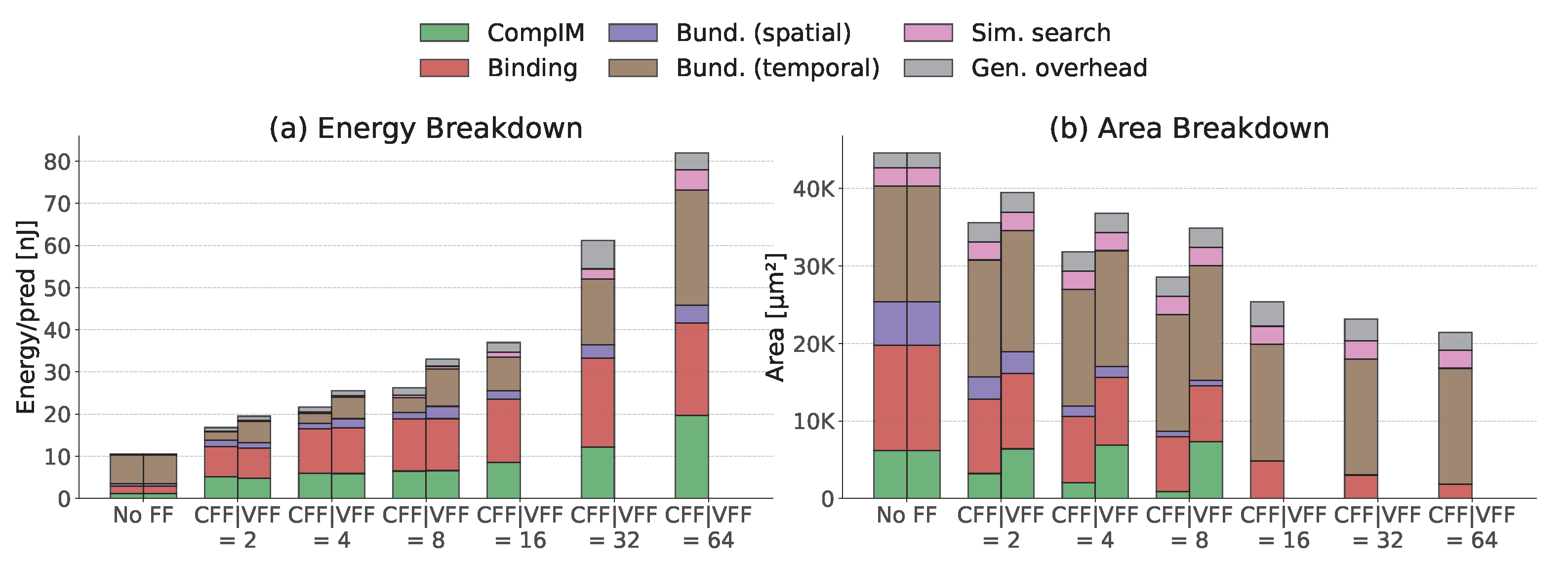
In the streamlined architecture, we systematically evaluate the performance trade-offs of sequentialization by comparing CF and VF, as depicted in Figure 8. These sequentialization techniques effectively trade silicon area reduction for increased energy consumption as depicted in Figure 14, which occurs because latency scales proportionally with the selected folding factor. However, for any given folding factor, CF proves to be more efficient than VF in terms of both area and energy. The area advantage stems directly from how each technique interacts with the CompIM. While VF must retain the entire compressed HV data for every channel, even when only a fraction is used per cycle, CF completely reuses its CompIM instances for the next set of channels. Thus, CF allows the CompIM footprint to shrink efficiently, whereas the CompIM size in VF remains restrictively large despite folding. Additionally, CF achieves lower energy consumption than VF due to reduced switching activity in the temporal bundling module; unlike VF, which triggers this module every clock cycle, CF does not because of the extra register after the spatial bundling. Finally, scaling to higher folding factors becomes less attractive because the temporal bundling area cannot shrink from folding, and the overall energy continues to rise due to the increased latency.
Conversely, applying these folding strategies to the IM-free architecture yields counterproductive results as seen in Figure 15. Rather than decreasing the footprint, sequentialization actually increases the total area in this design. This regression occurs because the additional FSM logic required in the binding module to manage the sequentialized electrode HVs outweighs any area saved elsewhere. Furthermore, in the highly optimized IM-free configuration, the temporal bundling module becomes the dominant hardware bottleneck. Because CF and VF do not fundamentally reduce the size of this specific module, sequentialization fails to provide any meaningful area benefit.
Ultimately, this analysis shows that while the streamlined architecture can effectively leverage sequentialization to reduce its silicon footprint, the folding factor should not be set excessively high. Because the relative area gains quickly diminish against steep energy and latency penalties, a moderate approach is necessary. Consequently, we use a CFF of 4, which provides a balance between the area benefit and the resulting energy penalty. In contrast, the IM-free architecture cannot utilize CF or VF in any meaningful capacity. Therefore, in the subsequent section, we benchmark our two most competitive and balanced configurations against the current SotA: the streamlined architecture utilizing a CFF of 4, and the IM-free architecture without any folding.

5.3. State-of-the-Art Comparison

To thoroughly evaluate our proposed optimizations, Table 2 benchmarks our work against three distinct groups of SotA hardware: sparse HDC accelerators across various applications, dense HDC accelerators, and non-HDC machine learning accelerators specifically targeting EEG/iEEG classification tasks. We present our results using two final configurations of our architecture: an energy-optimized design (IM-free) that maximizes dynamic energy savings within our explored design space, and a balanced design utilizing a CFF of 4 that balances energy and area while outperforming the IM-free architecture algorithmically. We normalize the data to the technology node and supply voltage with the empirically derived formulas from [11].
When comparing our architecture against other HDC systems, it is crucial to normalize the energy consumption for a fair comparison. This normalization accounts for the technology node and supply voltage [11], as well as inherent HDC parameters, including HV dimension (D), the number of processed HVs per prediction, and a baseline density of 1% for sparse implementations. Under this rigorous normalization, our energy-optimized design achieves a normalized energy of just 0.418 fJ per prediction. This significantly outperforms the most efficient competing sparse HDC design [8], which operates at 3.08 fJ, as well as other sparse implementations like [7], which consumes 510 fJ. Furthermore, achieving 0.418 fJ demonstrates orders-of-magnitude energy improvements over the dense HDC baselines, which require 14.0 fJ [12] and up to 1100 fJ [14] per prediction.
Because non-HDC implementations lack analogous structural HDC parameters, we compare them against our design by normalizing energy solely to the technology node and supply voltage. Even against highly optimized traditional machine learning accelerators for EEG/iEEG, our system demonstrates vastly superior energy efficiency. Traditional architectures demand high energy per prediction, such as 33.4 nJ for a convolutional neural network (CNN) [17], 600 nJ for a spiking neural network (SNN) [16], and up to 26,000 nJ for a support-vector-machine (SVM) architecture [15]. In stark contrast, our architecture operates at a fundamentally lower energy envelope, requiring only 7.01 nJ. This demonstrates that our algorithmic–hardware co-design is well-suited to the strict energy constraints of edge devices.
While the IM-free architecture achieves the absolute minimum hardware footprint and energy consumption, this extreme optimization comes with a slight penalty to algorithmic detection accuracy. To prioritize clinical performance, our balanced design utilizes the streamlined CompIM architecture, which preserves higher detection accuracy. Because this architecture is inherently larger, we leverage sequentialization to compress its silicon footprint. When normalized to the technology node, this balanced design achieves an area of 0.036 mm2. Although slightly larger than the IM-free configuration, it remains substantially smaller than competing sparse HDC accelerators, such as [8] at 690 mm2, and is highly competitive with dense HDC implementations, which range from 0.26 mm2 [14] down to 0.03 mm2 [12]. Ultimately, this balanced configuration represents an optimal trade-off, delivering SotA area and energy efficiency without sacrificing the algorithmic accuracy required for reliable iEEG seizure detection.

6. Conclusions

By systematically co-optimizing the HDC encoding architecture for sparsity, this work resolves the severe area and energy bottlenecks typically associated with high-dimensional vector processing in edge-based iEEG monitors. We demonstrate that when accuracy can be slightly relaxed, traditional IMs can be entirely bypassed by mapping raw LBP features directly to standard shift binding operations, fundamentally altering the hardware footprint. Quantitatively, this energy-optimized IM-free approach achieves 5.55× area and 3.08× energy improvements over the sparse baseline, corresponding to 8.20× and 13.37× improvements over standard dense HDC. Furthermore, our analysis of sequentialization trade-offs reveals that applying a CFF of 4 provides an optimal balance for clinical efficacy. This configuration preserves high detection accuracy while still delivering a 5.97× area and 4.66× energy reduction over the dense baseline, incurring a 4× latency penalty. Ultimately, these customizable hardware profiles prove that sparse HDC can be practically scaled for always-on, implantable neural interfaces.

Author Contributions

Conceptualization, S.C., R.A. and M.V.; methodology, S.C. and R.A.; software, S.C.; validation, S.C.; formal analysis, S.C.; investigation, S.C.; resources, M.V.; data curation, S.C.; writing—original draft preparation, S.C.; writing—review and editing, S.C., R.A., C.F. and M.V.; visualization, S.C.; supervision, C.F. and M.V.; project administration, S.C. and C.F.; funding acquisition, M.V. All authors have read and agreed to the published version of the manuscript.

Funding

This project has been partly funded by the European Research Council (ERC) under grant agreement No. 101088865, the European Union’s Horizon 2020 program under grant agreement No. 101070374, the Flanders AI Research Program, and long-term structural Methusalem funding by the Flemish Government.

Data Availability Statement

The original data presented in the study are openly available in KULeuven-MICAS/sparse_HDC_for_iEEG at https://github.com/KULeuven-MICAS/sparse_HDC_for_iEEG (accessed on 10 April 2026).

Acknowledgments

During the preparation of this manuscript/study, the author(s) used Google Gemini (Gemini 3.1 Pro) for the purposes of generating text. The authors have reviewed and edited the output and take full responsibility for the content of this publication.

Conflicts of Interest

The authors declare no conflicts of interest. The funders had no role in the design of the study; in the collection, analyses, or interpretation of data; in the writing of the manuscript; or in the decision to publish the results.

References

  1. Kleyko, D.; Rachkovskij, D.A.; Osipov, E.; Rahimi, A. A Survey on Hyperdimensional Computing aka Vector Symbolic Architectures, Part I: Models and Data Transformations. ACM Comput. Surv. 2022, 55, 1–40. [Google Scholar] [CrossRef] [Scilit]
  2. Burrello, A.; Schindler, K.; Benini, L.; Rahimi, A. One-shot Learning for iEEG Seizure Detection Using End-to-end Binary Operations: Local Binary Patterns with Hyperdimensional Computing. In Proceedings of the 2018 IEEE Biomedical Circuits and Systems Conference (BioCAS); IEEE: New York, NY, USA, 2018; pp. 1–4. [Google Scholar] [CrossRef] [Scilit]
  3. Cumbo, F.; Chicco, D. Hyperdimensional Computing in Biomedical Sciences: A brief review. PeerJ Comput. Sci. 2025, 11, e2885. [Google Scholar] [CrossRef] [Scilit]
  4. Kleyko, D.; Rachkovskij, D.; Osipov, E.; Rahimi, A. A Survey on Hyperdimensional Computing aka Vector Symbolic Architectures, Part II: Applications, Cognitive Models, and Challenges. ACM Comput. Surv. 2023, 55, 1–52. [Google Scholar] [CrossRef] [Scilit]
  5. Cuyckens, S.; Antonio, R.; Fang, C.; Verhelst, M. iEEG Seizure Detection with a Sparse Hyperdimensional Computing Accelerator. In Proceedings of the 2025 20th International Conference on PhD Research in Microelectronics and Electronics (PRIME); IEEE: New York, NY, USA, 2025; pp. 1–4. [Google Scholar] [CrossRef] [Scilit]
  6. Galapon, F.A.R.; Alvarez, A.B. A Hyperdimensional Computing Architecture with 4.4x Energy Efficiency in 65nm CMOS. In Proceedings of the 2024 IEEE International Symposium on Circuits and Systems (ISCAS); IEEE: New York, NY, USA, 2024; pp. 1–5. [Google Scholar] [CrossRef] [Scilit]
  7. Imani, M.; Hwang, J.; Rosing, T.; Rahimi, A.; Rabaey, J.M. Low-Power Sparse Hyperdimensional Encoder for Language Recognition. IEEE Des. Test 2017, 34, 94–101. [Google Scholar] [CrossRef] [Scilit]
  8. Buelagala, K.I.I.; Javier, G.S.; Lipardo, S.A.A.; Sorsona, J.C.E.; Baquiran, S.J.A.S.; Quizon, L.R.A.; Tan, A.J.A.; Antonio, R.A.G.; Galapon, F.A.R.; Alvarez, A.B. Energy-Efficient Sparse Hyperdimensional Computing for Speech Recognition. In Proceedings of the 2023 20th International SoC Design Conference (ISOCC); IEEE: New York, NY, USA, 2023; pp. 321–322. [Google Scholar] [CrossRef] [Scilit]
  9. Hersche, M.; Rella, E.M.; Di Mauro, A.; Benini, L.; Rahimi, A. Integrating event-based dynamic vision sensors with sparse hyperdimensional computing: A low-power accelerator with online learning capability. In Proceedings of the ACM/IEEE International Symposium on Low Power Electronics and Design; Association for Computing Machinery: New York, NY, USA, 2020; ISLPED ’20; pp. 169–174. [Google Scholar] [CrossRef] [Scilit]
  10. Justus Rajappa, A.; Smets, L.; Reiter, P.; Rech, P.; Vanderhoydonc, Y.; Singh, R.K.; Mercelis, S.; Famaey, J. Optimized Hyperdimensional Edge AI Evaluation for Efficiency and Reliability under Real Radiation. ACM Trans. Embed. Comput. Syst. 2026, 25, 1–24. [Google Scholar] [CrossRef] [Scilit]
  11. Stillmaker, A.; Baas, B. Scaling equations for the accurate prediction of CMOS device performance from 180 nm to 7 nm. Integration 2017, 58, 74–81. [Google Scholar] [CrossRef] [Scilit]
  12. Menon, A.; Sun, D.; Sabouri, S.; Lee, K.; Aristio, M.; Liew, H.; Rabaey, J.M. A Highly Energy-Efficient Hyperdimensional Computing Processor for Biosignal Classification. IEEE Trans. Biomed. Circuits Syst. 2022, 16, 524–534. [Google Scholar] [CrossRef] [Scilit]
  13. Khaleghi, B.; Kang, J.; Xu, H.; Morris, J.; Rosing, T. Generic: Highly efficient learning engine on edge using hyperdimensional computing. In Proceedings of the 59th ACM/IEEE Design Automation Conference; Association for Computing Machinery: New York, NY, USA, 2022; pp. 1117–1122. [Google Scholar]
  14. Eggimann, M.; Rahimi, A.; Benini, L. A 5 μW standard cell memory-based configurable hyperdimensional computing accelerator for always-on smart sensing. IEEE Trans. Circuits Syst. I Regul. Pap. 2021, 68, 4116–4128. [Google Scholar] [CrossRef] [Scilit]
  15. de Bruin, B.; Singh, K.; Huisken, J.; Corporaal, H. BrainWave: An energy-efficient EEG monitoring system—Evaluation and trade-offs. In Proceedings of the ACM/IEEE International Symposium on Low Power Electronics and Design; Association for Computing Machinery: New York, NY, USA, 2020; ISLPED ’20; pp. 181–186. [Google Scholar] [CrossRef] [Scilit]
  16. Zhang, Q.; Cui, M.; Liu, Y.; Chen, W.; Yu, Z. Low-Power and Low-Cost AI Processor With Distributed-Aggregated Classification Architecture for Wearable Epilepsy Seizure Detection. IEEE Trans. Biomed. Circuits Syst. 2025, 19, 28–39. [Google Scholar] [CrossRef] [Scilit]
  17. Shi, W.; Qin, H.; Wu, J.; Mai, J. Design of a CNN Accelerator for Multitask EEG Signal Classification Based on RISC-V. IEEE Trans. Very Large Scale Integr. VLSI Syst. 2025, 33, 2630–2638. [Google Scholar] [CrossRef] [Scilit]
  18. Zhao, S.; Yang, J.; Wang, J.; Fang, C.; Liu, T.; Zhang, S.; Sawan, M. A 0.99-to-4.38 uJ/class Event-Driven Hybrid Neural Network Processor for Full-Spectrum Neural Signal Analyses. IEEE Trans. Biomed. Circuits Syst. 2023, 17, 598–609. [Google Scholar] [CrossRef] [Scilit]
  19. Schlegel, K.; Neubert, P.; Protzel, P. A comparison of vector symbolic architectures. Artif. Intell. Rev. 2022, 55, 4523–4555. [Google Scholar] [CrossRef] [Scilit]
  20. Imani, M.; Kong, D.; Rahimi, A.; Rosing, T. VoiceHD: Hyperdimensional Computing for Efficient Speech Recognition. In Proceedings of the 2017 IEEE International Conference on Rebooting Computing (ICRC); IEEE: New York, NY, USA, 2017; pp. 1–8. [Google Scholar] [CrossRef] [Scilit]
  21. Rahimi, A.; Benatti, S.; Kanerva, P.; Benini, L.; Rabaey, J.M. Hyperdimensional biosignal processing: A case study for EMG-based hand gesture recognition. In Proceedings of the 2016 IEEE International Conference on Rebooting Computing (ICRC); IEEE: New York, NY, USA, 2016; pp. 1–8. [Google Scholar] [CrossRef] [Scilit]
  22. Rachkovskij, D.A.; Kussul, E.M. Binding and Normalization of Binary Sparse Distributed Representations by Context-Dependent Thinning. Neural Comput. 2001, 13, 411–452. [Google Scholar] [CrossRef] [Scilit]
  23. Laiho, M.; Poikonen, J.H.; Kanerva, P.; Lehtonen, E. High-dimensional computing with sparse vectors. In Proceedings of the 2015 IEEE Biomedical Circuits and Systems Conference (BioCAS); IEEE: New York, NY, USA, 2015; pp. 1–4. [Google Scholar] [CrossRef] [Scilit]
  24. Fishbein, J.M.; Eliasmith, C. Integrating Structure and Meaning: A New Method for Encoding Structure for Text Classification. In Proceedings of the Advances in Information Retrieval; Macdonald, C., Ounis, I., Plachouras, V., Ruthven, I., White, R.W., Eds.; Springer: Berlin/Heidelberg, Germany, 2008; pp. 514–521. [Google Scholar]
  25. Hersche, M.; Zeqiri, M.; Benini, L.; Sebastian, A.; Rahimi, A. A neuro-vector-symbolic architecture for solving Raven’s Progressive Matrices. Nat. Mach. Intell. 2023, 5, 363–375. [Google Scholar] [CrossRef] [Scilit]
  26. Smets, L.; Van Leekwijck, W.; Tsang, I.J.; Latré, S. An encoding framework for binarized images using hyperdimensional computing. Front. Big Data 2024, 7, 1371518. [Google Scholar] [CrossRef] [Scilit]
  27. Pale, U.; Teijeiro, T.; Atienza, D. ExG Signal Feature Selection Using Hyperdimensional Computing Encoding. In Proceedings of the 2022 IEEE International Conference on Bioinformatics and Biomedicine (BIBM); IEEE: New York, NY, USA, 2022; pp. 1688–1693. [Google Scholar] [CrossRef] [Scilit]
  28. The SWEC-ETHZ iEEG Database and Algorithms—IEEG-swez.ethz.ch. Available online: http://ieeg-swez.ethz.ch/ (accessed on 24 February 2026).
  29. Schmuck, M.; Benini, L.; Rahimi, A. Hardware Optimizations of Dense Binary Hyperdimensional Computing: Rematerialization of Hypervectors, Binarized Bundling, and Combinational Associative Memory. J. Emerg. Technol. Comput. Syst. 2019, 15, 1–25. [Google Scholar] [CrossRef] [Scilit]
  30. Khaleghi, B.; Xu, H.; Morris, J.; Rosing, T.Š. tiny-HD: Ultra-Efficient Hyperdimensional Computing Engine for IoT Applications. In Proceedings of the 2021 Design, Automation & Test in Europe Conference & Exhibition (DATE); IEEE: New York, NY, USA, 2021; pp. 408–413. [Google Scholar] [CrossRef] [Scilit]
  31. Yu, T.; Wu, B.; Chen, K.; Zhang, G.; Liu, W. Fully Learnable Hyperdimensional Computing Framework With Ultratiny Accelerator for Edge-Side Applications. IEEE Trans. Comput. 2024, 73, 574–585. [Google Scholar] [CrossRef] [Scilit]
  32. Menon, A. Neural Prosthetic with in-Sensor Shared Control. Ph.D. Thesis, University of California, Berkeley, CA, USA, 2022. [Google Scholar]
  33. Sun, D. Low-Power Hyperdimensional Computing Processors for Real-Time Wearable Sensor Fusion and Keyword Classification. Available online: https://www2.eecs.berkeley.edu/Pubs/TechRpts/2022/EECS-2022-118.pdf (accessed on 10 April 2026).
  34. Menon, A.; Natarajan, A.; Agashe, R.; Sun, D.; Aristio, M.; Liew, H.; Shao, Y.S.; Rabaey, J.M. Efficient emotion recognition using hyperdimensional computing with combinatorial channel encoding and cellular automata. Brain Inform. 2022, 9, 14. [Google Scholar] [CrossRef] [Scilit] [PubMed]
  35. Datta, S.; Antonio, R.A.G.; Ison, A.R.S.; Rabaey, J.M. A Programmable Hyper-Dimensional Processor Architecture for Human-Centric IoT. IEEE J. Emerg. Sel. Top. Circuits Syst. 2019, 9, 439–452. [Google Scholar] [CrossRef] [Scilit]
  36. Sze, V.; Chen, Y.H.; Yang, T.J.; Emer, J.S. Efficient processing of deep neural networks: A tutorial and survey. Proc. IEEE 2017, 105, 2295–2329. [Google Scholar] [CrossRef] [Scilit]
  37. Kanerva, P. Hyperdimensional computing: An introduction to computing in distributed representation with high-dimensional random vectors. Cogn. Comput. 2009, 1, 139–159. [Google Scholar] [CrossRef] [Scilit]
  38. Angioli, M.; Kymn, C.J.; Rosato, A.; Loutfi, A.; Olivieri, M.; Kleyko, D. Efficient Hyperdimensional Computing with Modular Composite Representations. arXiv 2025, arXiv:2511.09708. [Google Scholar] [CrossRef] [Scilit]
  39. Martino, R.; Pisani, M.; Angioli, M.; Barbirotta, M.; Mastrandrea, A.; Rosato, A.; Olivieri, M. A General-Purpose AXI Plug-and-Play Hyperdimensional Computing Accelerator. Electronics 2026, 15, 489. [Google Scholar] [CrossRef] [Scilit]
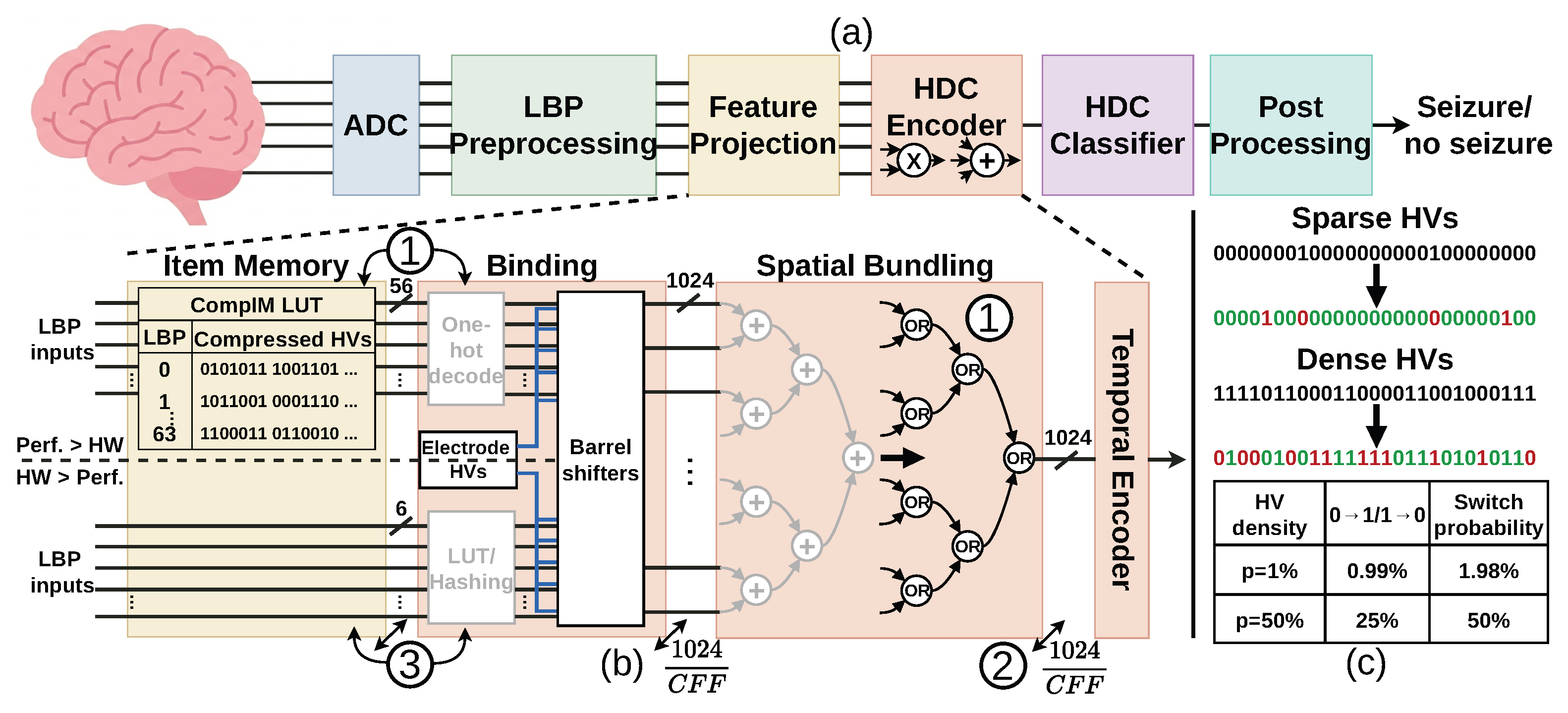
Figure 1. Overview figure. (a) Intracranial electroencephalography (iEEG) seizure detection system with hyperdimensional computing (HDC) and local binary pattern (LBP) codes; (b) item memory and spatial HDC encoder with our 3 contributions: (1) streamlined architecture with compressed item memory (CompIM) and simplified spatial bundling, (2) channel folding with a channel folding factor (CFF), and (3) the item-memory-free (IM-free) architecture; (c) switching activity comparison of dense high-dimensional vectors (HVs) and sparse HVs.
Chips 05 00010 g001
Figure 2. Example of the binding, bundling, and permutation operation. (a) Feature-value hypervectors are bound (⊗) to form specific traits, which are then bundled (⊕) to represent a single dog. (b) The permutation operator ( ρ , ρ 2 ) encodes the dogs’ respective positions on the podium, which are bundled to represent the winners of the race.
Chips 05 00010 g002
Figure 3. General hyperdimensional computing algorithm structure.
Chips 05 00010 g003
Figure 4. Examples of hypervector (HV) operations. (a) Segmented shift binding, (b) shift binding, and (c) bundling with thinning strategies: segmented thinning, threshold thinning, and context-dependent thinning (CDT).
Chips 05 00010 g004
Figure 5. The iEEG seizure detection algorithm utilizing local binary pattern (LBP) codes and hyperdimensional computing with look-up tables, storing the hypervectors (HVs) and storing class-representing HVs in the associative memory (AM).
Chips 05 00010 g005
Figure 6. An example of (a) the local binary pattern (LBP) and (b) the predictions of a seizure. First, there is 3 min of normal data (prediction of 0), then the seizure starts at 180 s. The system should output 1-bits, often with some 0-bits at the start that extend the time before the seizure is detected. Wrong predictions are indicated in red, right seizure predictions are indicated in green.
Chips 05 00010 g006
Figure 7. Overview of (a) the hardware implementation of the item memory (IM), converting local binary pattern (LBP) codes into high-dimensional vectors (HVs), and the hyperdimensional computing (HDC) encoder for the sparse baseline; (b) the optimized sparse implementation with segmented shift binding, using the compressed item memory (CompIM) and simplified spatial bundling optimizations. (c) The area and energy breakdown of the sparse baseline. The diagonal arrows indicate that there are parallel units of the block; the lowercase letters d, e, and s indicate the dimension of the HVs, electrodes, and the segments of an HV, respectively.
Chips 05 00010 g007
Figure 8. (a) The optimized segmented shift binding accelerator with a channel folding factor (CFF) of 4 and (b) a vector folding factor (VFF) of 4. (c) Channel and vector folding are also represented in the nested for-loop notation.
Chips 05 00010 g008
Figure 9. (a) The baseline hyperdimensional computing (HDC) implementation with shift binding, using a look-up table (LUT) or hashing function in the binding unit; (b) the optimized implementation with shift binding, where the item memory (IM) and LUT/hashing function have been removed.
Chips 05 00010 g009
Figure 10. The core concept of our item-memory-free (IM-free) architecture for shift binding. The normal path, requiring an item memory (IM) to convert local binary pattern (LBP) codes to hypervectors (HVs) and a look-up-table (LUT) to convert the HVs to shift values, is indicated in black, and our optimized path, bypassing all of this, is indicated in blue.
Chips 05 00010 g010
Figure 11. (a) Confusion matrix with a similarity score between an original electrode memory (EM) hypervector (HV) and its shifted version, averaged over all 64 HVs of the EM. (b) Mean off-diagonal similarity score averaged over the 64 HVs of the EM and over the shifts from 0 to 63 with dimensionality between 512 and 8192. The similarity score when limiting the shifts is compared to the similarity score of randomly generated orthogonal HVs and to the same EM but with randomly selected shifts between 0 and D.
Chips 05 00010 g011
Figure 12. Average seizure detection delay and detection accuracy for varying densities after bundling. Data is averaged over 4 pairs of item memory hypervectors (HVs) and electrode HVs, showing the effect of our compressed item memory (CompIM), simplified spatial bundling (thin. opt.), and item-memory-free (IM-free) optimizations on the algorithmic performance [2].
Chips 05 00010 g012
Figure 13. Energy and area breakdown of our streamlined architecture with the compressed item memory (CompIM) and simplified spatial bundling (thin. opt.), and item-memory-free (IM-free) architectures with improvement factors relative to the dense HDC baseline.
Chips 05 00010 g013
Figure 14. Energy and area breakdown of the streamlined architecture with vector and channel folding factors (VFF and CFF).
Chips 05 00010 g014
Figure 15. Energy and area breakdown of the item-memory-free (IM-free) architecture with vector and channel folding factors (VFFs and CFFs).
Chips 05 00010 g015
Table 1. Energy and area efficiency comparison with sparse hyperdimensional computing state-of-the-art accelerators. The energy from [6,9] could not be normalized as the number of hypervectors (HVs) per prediction varies.
Energy/pred.Energy impr.Norm. Energy/pred. *Area (mm2)Norm. Area (mm2) *
Language recog [7].Dense/////
Sparse///−34%/
Language recog [6].Dense240 nJ////
Sparse45 nJ×4.40/−3.68%/
Event vision [9]Dense5.2 μ J////
Sparse5.0 μ J×1.04///
Speech recog [8].Dense/////
Sparse34.05 nJ/2.79 fJ755172.5
iEEG seizure (our foundational work) [5]Dense93.75 nJ/5.72 fJ0.190.19
Sparse21.5 nJ×4.361.31 fJ0.130.13
Sparse
optim.
12.5 nJ×7.500.763 fJ0.0590.059
* Normalized energy is scaled by technology node and supply voltage as in [11], number of HVs per prediction, HV dimension, and density. Normalized area is scaled by technology node and normalized to an HV dimension of 1024. In bold, we indicate the only state-of-the-art work using optimizations to highlight its superior energy and area efficiency.
Table 2. Comparison with state-of-the-art works, with “D” being the number of dimensions in the hypervectors (HVs) and “d” the density of the HVs. Our item-memory-free (IM-free) and streamlined architecture with a channel folding factor (CFF) of 4 are indicated in bold.
WorkApp.Alg.HWTech 
(nm)
Vdd 
(V)
Freq. 
(MHz)
D
(%)
HVs/OutputArea 
( mm 2 )
Latency/ 
pred
Energy/ 
pred 
( nJ )
Norm. 
Area 
( mm 2 )  a
Norm. 
Latency a
Norm. 
Energy 
( nJ )  a
Norm. 
Energy 
( fJ )  b
Det. 
Acc. 
(%)
Sparse HDC works
IM-freeiEEGSparseASIC160.76101k116,3840.02325.6 μ s7.010.02325.6 μ s7.010.41898.6
str. arch. CFFiEEGSparseASIC160.75101k116,3840.036102.4 μ s20.10.036102.4 μ s20.11.2099.1
[5]iEEGSparseASIC160.75101k≈116,3840.05925.6 μ s12.50.05925.6 μ s12.50.75/
[7]Lang.SparseASIC451.0-10k4--48.4 ns--52 ns-510/
[6]Lang.SparseASIC651.010010k1---45.0--2.96-/
[9]VisionSparse-551.21008k----5000--210-/
[8]SpeechSparseASIC22-504k2617755-34.1690-15.63.08/
Dense HDC works
[12]ExGDenseASIC280.80.912k502140.0681 ms39.10.030.15 ms7.5114.0/
[13]Gen.DenseASIC14-5002k50-0.30.1 ms10.00.30.1 ms10.0-/
[14]EMGDenseASIC220.8<0.12k50640.29500 ms1910.260.03 ms-1100/
iEEG works
[15]EEGSVMCGRA280.9100----47.8 ms160,000-11.0 ms26,000-/
[16]EEGSNNFPGA28-100----171 ms3730-39.2 ms600-/
[18]ExGS/ANNASIC550.750.3---6.286.94 ms9900.792.65 ms110-/
[17]EEGCNNASIC401.010---0.421.82 ms3280.081.96 ms33.4-/
a The data is normalized to 16 nm technology and a supply voltage of 0.75 V according to [11]. b The data is normalized to technology and supply voltage [11], the HV dimension (D), the number of HVs processed per output, and a density of 1% for the sparse HDC papers.
Disclaimer/Publisher’s Note: The statements, opinions and data contained in all publications are solely those of the individual author(s) and contributor(s) and not of MDPI and/or the editor(s). MDPI and/or the editor(s) disclaim responsibility for any injury to people or property resulting from any ideas, methods, instructions or products referred to in the content.