Statistical Analysis of Measurement Processes Using Multi-Physic Instruments: Insights from Stitched Maps

Abstract

Stitching methods allow one to measure a wider surface without the loss of resolution. The observation of small details with a better topographical representation is thus possible. However, it is not excluded that stitching methods generate some errors or aberrations on topography reconstruction. A device including confocal microscopy (CM), focus variation (FV), and coherence scanning interferometry (CSI) instrument modes was used to chronologically follow the drifts and the repositioning errors on stitching topographies. According to a complex measurement plan, a wide measurement campaign was performed on TA6V specimens that were ground with two neighboring SiC FEPA grit papers (P#80 and P#120). Thanks to four indicators (quality, drift, stability, and relevance indexes), no measurement drift in the system was found, indicating controlled stitching and repositioning processes for interferometry, confocal microscopy, and focus variation. Measurements show commendable stability, with interferometric microscopy being the most robust, followed by confocal microscopy, and then focus variation. Despite variations, robustness remains constant for each grinding grit, minimizing interpretation biases. A bootstrap analysis reveals time-dependent robustness for confocal microscopy, which is potentially linked to human presence. Despite Sa value discrepancies, all three metrologies consistently discriminate between grinding grits, highlighting the reliability of the proposed methodology.

1. Introduction

In the field of manufacturing, the comprehension of the process and the surface specifications take on ever greater importance due to needs in micro-mechanism design [1], bio-mechanisms [2], and system performance optimization [3] and reliability [4]. This underscores the importance of characterizing surfaces through topographic measurements to analyze their overview and observe known physical phenomena. The surface topography investigation mainly depends on magnification (scale), the (X, Y, Z) resolution, and the field of view (topographic representativeness). But sometimes, a single measurement is not sufficient to observe surfaces because a choice needs to be made between the details and topographic representativeness [5]. It is for this reason that stitching is employed in the surface topography measurement.

Stitching is a process of combining and merging a set of neighboring elementary maps sharing overlapping zones [6]. The measured zones which compose the stitch (elementary maps) are scanned following a specific method (regular, serpentine) with (X, Y) displacements between maps corresponding to an overlapping value. The positioning of maps is most often made according to table coordinates (X, Y) and using a method of Z optimization to minimize the ΔZ.

As introduced before, stitching methods slightly modify the surfaces due to the positioning (six degrees of freedom) and the blending method of maps. As explained by Lemesle et al. [7], six methods of in-plan registration are found in the literature: manual, geometric, fiducialization, global optimization of differences, computer vision-based (direct method), and computer vision-based (feature detection method), as shown in Table 1. These methods are detailed below:

• The manual method is simply made by the user. It can use the forms, the outline of shapes, and the features to match the surface. But this method depends on the user’s perception and is time consuming.
• The geometric method is based on the table coordinate and also depends on the table precision (XY). The positions can be relative between maps (XY displacement) or absolute given by the table. This method is directly performed by the software and is simple and faster than the manual method. But it is not uncommon for stitching errors to occur.
• The fiducialization method uses micro-machined markers directly on the surface to collocate maps for the stitching. This method can be sensitive to the measuring errors of markers and the quality of repositioning. Nevertheless, this method is simple and precise but results in a loss of surface integrity.
• The global optimization of differences method is based on minimization criteria and thus depends on the minimization method and the topography landscape. Even though this method can limit the stitching errors and has a fast solving process, it can be difficult to apply in certain cases (flat surfaces with autocorrelated noise).
• The direct computer vision-based method is based on similarity detection (as the cross correlation) and is carried out on all pixels of the overlapping areas of stitched maps. This method is influenced by the measurement noise and the landscape of surface topographies. This method is very precise but cannot be applied on very large surfaces (due to the number of points).
• The computer vision-based method with feature detection is similar to the direct method but takes into account edges, corners, or blobs to find points of interest (POI) on maps with algorithms, as explained by Prathap et al. [8]. These algorithms, called detectors and descriptors, are used to find these features on maps. Several detectors exist, such as Harris Corner [9] and FAST [10]; several descriptors also exist, such as SIFT [11], SURF [11,12], BRIEF [9], BRISK [13], ORB [14], and FREAK [15]. The difference between them is that detectors just detect the POI, while descriptors detect, compare, and match the POI. In the matching process, random sample consensus (RANSAC) [16] is always used to eliminate mismatching POI and select the most relevant POI. This method is very precise but cannot be applied on very small surfaces (due to the insufficient POI) and may give different results for a given configuration (two elementary maps).

More generally, the presented methods are all sensible to the quality of measurement, the resolution, and the technology of the instrument.

Table 1. Summary of registration methods in the plan for stitching with their criteria, dependencies, strengths, and weaknesses.

Method	Processed by	Based on	Dependence on	Strengths	Weaknesses
Manual	The user	Forms, outline of shapes, and features	Human perception	The user controls the stitch	Time consuming, cannot be automated
Geometric	The software	The device coordinate	Device precision (XY table)	Simple and faster than other methods	Stitching errors can appear
Fiducialization	The user and the software	Markers or specific forms micro-machined on surface	Quality of repositioning and marker measurement errors	Simple and precise	Loss of surface integrity
Global optimization of differences	The software	A minimization of difference (XY)	Minimization method and surface topographies	Limit the errors on stitched maps, solving process faster	Can be difficult to convey in certain applications
Computer vision-based (direct method)	The software	The similarities between two surfaces using all pixels	Measurement noise and surface topographies	Very precise	Difficult to apply on large maps and time consuming
Computer vision-based (feature detection method)	The software	The similarities between two surfaces using descriptors			Difficult to apply on small maps, can give different results due to RANSAC, and time consuming

Table 1. Summary of registration methods in the plan for stitching with their criteria, dependencies, strengths, and weaknesses.

Method	Processed by	Based on	Dependence on	Strengths	Weaknesses
Manual	The user	Forms, outline of shapes, and features	Human perception	The user controls the stitch	Time consuming, cannot be automated
Geometric	The software	The device coordinate	Device precision (XY table)	Simple and faster than other methods	Stitching errors can appear
Fiducialization	The user and the software	Markers or specific forms micro-machined on surface	Quality of repositioning and marker measurement errors	Simple and precise	Loss of surface integrity
Global optimization of differences	The software	A minimization of difference (XY)	Minimization method and surface topographies	Limit the errors on stitched maps, solving process faster	Can be difficult to convey in certain applications
Computer vision-based (direct method)	The software	The similarities between two surfaces using all pixels	Measurement noise and surface topographies	Very precise	Difficult to apply on large maps and time consuming
Computer vision-based (feature detection method)	The software	The similarities between two surfaces using descriptors			Difficult to apply on small maps, can give different results due to RANSAC, and time consuming

The stitching algorithms are based on both surface features [17] and images of topography or reflectance [7]. As explained before, the main stitching challenge is to match two overlapping areas of elementary maps to build a bigger surface with a maximum of similarities. But neighboring maps are different due to noise [18] or measurement point-of view, and have a shift of positioning reference due to (X/Y) table drifts or uncertainties due to the influence of the environment on instrument measurement conditions. This is why stitching can introduce errors as shown in [19]. The stitching errors depend firstly on the elementary maps coming from the instrument: resolution, overlapping percentage, or type of technology. As shown in [20], distortions of elementary maps exist which may cause stitching errors. The uncertainties due to the height fluctuation of the pixels caused by local slopes, as shown in [21], can also cause mismatches. The measurement noise [22], the XYZ scale [23], or the resolution as in [24] can also generate uncertainties on elementary maps and thus stitching misalignments. The environment factors can also be a cause of stitching errors. As introduced before, the instrument technology can generate their own stitching errors. Paul et al. [25] showed a 10 nm error appears on a lithography measurement of 10 µm × 10 µm with an AFM. But the instrument is sometimes not the only source of errors. Lemesle et al. [7] showed through mean repositioning error (MRE, based on ΔX and ΔY off-set) and stitching error estimator (SEE, based on p-value) that the stitching algorithms can generate errors and these errors also depend on the stitching method and the type of stitched surface. The MRE indicator gives errors to the order of several tenths of a pixel and the SEE indicator gives errors from −1.17 to −0.36.

When conducting a stitched measurement study, it is essential to consider not only the instruments and the measurement conditions. Indeed, the stitched surfaces are characterized through roughness parameters such as the Sa parameter or others defined by the ISO 25178-2 standard [26]. However, as stitched surfaces are larger and have a greater number of points (conservation of lateral resolution) than elementary surfaces, the parameters can become less sensitive to statistical fluctuations on the surface but can be altered by errors due to the stitching algorithms. This is why Sa is chosen in this paper because it is less sensitive to the isolated local peaks. Stitching can therefore give greater importance to long wavelengths for Sa, but it can also enrich the number of characteristic topographical features for its calculation. The same reasoning can be made for other parameters such as Sdr or Sal, but it is important not to overlook the fact that blending areas can influence the calculation due to generated errors.

To assess the influence of each instrument on the measurement, an intercomparison between several instruments is needed and is based on a statistical method. This method is developed further; however, the question arises as to how an intercomparison should be carried out properly. Indeed, it is essential to know the conditions influencing the surfaces studied, i.e., surface type, functionalities, local properties, sample morphology, and relevant observation scale.

The intercomparison of optical profilometers is a common practice in the metrological field, as in [27,28,29]. All results coming from standard measurements obtained with different instruments need to be equivalent in accordance with filtering standards [30] and for an equivalent lateral sampling [31]. But in the scope of this paper, a filtering process is not necessary because it is assumed that the natural transfer function of instruments is taken into account in the comparison.

In addition, the comparisons made in the literature do not include indicators based on statistics showing the performances of discrimination between two neighboring surfaces through roughness parameters including simultaneously their relevance, stability, drift, and signal-to-noise ratio. A method previously developed by the authors [32] and initially applied on elementary topographical maps is applied here to stitched measurements.

Through this paper, the investigated method is used to show how novel statistical indicators (called indexes) allow the determination of whether an instrument is able to discriminate two ground surfaces having neighboring roughness. In addition, the measurements are stitched to determine if the stitching method can improve the quality (errors), allowing a more pronounced discrimination (relevance) to be shown, and determining if the quality of measurement impacts the discrimination between two ground surfaces having neighboring roughness.

2. Materials and Methods

2.1. Machining Specimens

In this study, a grinding process was chosen to machine TA6V rods. TA6V is used in aeronautic, chemical, and naval applications due to its mechanical properties (high strength, toughness, and lightness) and its corrosive resistance. These properties ensure the preservation of surface integrity during the comparison. The same operation of surface machining as in [32] was performed on the presented specimens. As illustrated in Figure 1, two 30 mm diameter TA6V rods were cut into 10 mm thick pieces. Following the cutting process, a pre-grinding step with a silicon carbide (SiC) grinding paper disc FEPA P#320 was taken to eliminate cutting marks and residual stresses. Subsequently, the specimens were ground with SiC papers ranging from P#80 grit to P#1200 grit to establish a consistent initial state for both samples. Each grinding step lasted 2 min with a rotational speed of 300 rpm and a normal force of 30 N, with the grinding papers being replaced at each stage. In the final phase, one TA6V specimen was ground with P#80 (#080), and the other one was ground with P#120 (#120). This final grinding step occurred over 15 min at 300 rpm, with a normal force of 30 N and water lubrication.

2.2. Measurement Conditions

2.2.1. Measurement Settings

The measurements were conducted using a Sensofar^® (Barcelona, Spain) S neox™ 3D optical profilometer (5th gen). This system employs various optical techniques, including focus variation, confocal, and interferometry. The shared optical path within the system’s internal design makes it well-suited for technology comparison studies. The only hardware distinction between the techniques is that focus variation and confocal utilize epi-illumination brightfield lenses and a monochromatic light source, while interferometry employs Michelson or Mirau interferometric lenses with either monochromatic or broadband light sources. The acquisition software provided with the system (SensoSCAN 7.10.1) provides a set of functionalities that allows the automatic stitching of multiple fields of view (FOV) into a single, larger area measurement. Also, multiple measurements can be programmed to be acquired automatically according to previously saved user-defined settings and measurement positions. The integration of three measurement technologies into a single device allows the same reference positioning system to be shared for each instrument mode and it can avoid the repositioning of the specimen between each mode switching, and thus can reduce the XY displacement of specimen to device uncertainties. It improves the relevance of the developed method. However, the method can be applied to a certain degree to other instruments (not necessarily multi-physic instruments).

For this study, a 20× magnification was chosen, with a numerical aperture (NA) of 0.45 for the brightfield objective and 0.40 for the interferometric one. The lateral resolution for the chosen configuration was 0.69 µm. The vertical resolution, described in terms of the measurement noise, was 8 nm for confocal and focus variation, and 1 nm for interferometry.

Each measurement was a result of stitching a 6-by-7 grid of individual measurements overlapped by 20%, covering a measurement area of 4.2 × 4.1 mm. The stitching path was serpentine. In this case, the tracking option “tilted surface or round shape” was used to take into account the tilt of the sample and maintain all the points within the selected measurement Z-range. This Z-range was set to 30 µm in the case of interferometry and 80 µm for the brightfield techniques. Regarding the stitching algorithm, the default options were selected for the XY and Z offsets, which means that the position of the individual fields of view was corrected when stitching was based on the optical image and also the 3D data. This compensated for the small hardware inaccuracies that occur when moving the XY stage, yielding a continuous surface. The measurement time for each acquisition was 2 min 25 s for confocal, 2 min 36 s for interferometry, and 2 min 46 s for focus variation.

2.2.2. Measurement Strategy

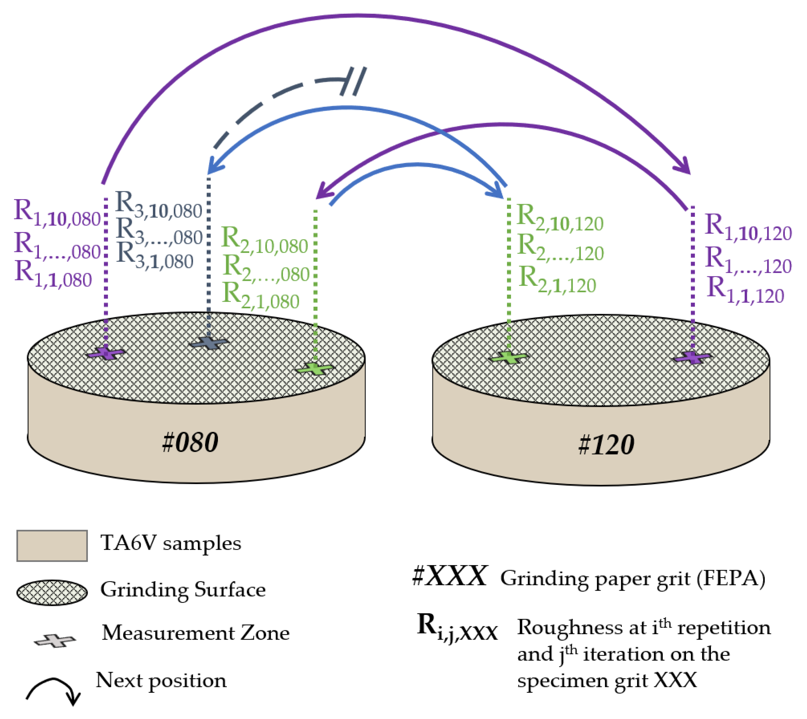
The steps of the measurement strategy are set out in Figure 2. The couple of specimens #080 and #120 were measured according to a specific measurement plan (Figure 3):

• 10 measurements at the first position on the specimen #080;
• 10 measurements at the first position on the specimen #120;
• 10 measurements at the second position on the specimen #080;
• 10 measurements at the second position on the specimen #120;
• And this, until the last position of each specimen.

The 10 measurements at a given position represent the iterations and the different positions represent the repetitions on the measurement plan. A notation was created to represent the measurement for a given step: $R_{i,j,XXX}$ with i the repetition number, j the iteration number, and XXX the specimen grit (#080 or #120). The measurement plan was based on the iteration and grit alternance to determine the global measurement quality (quality, drift, and stability) and the ability to discriminate both grits, #080 and #120 (relevance), respectively.

Figure 2. Scheme of measurement process steps.

Figure 2. Scheme of measurement process steps.

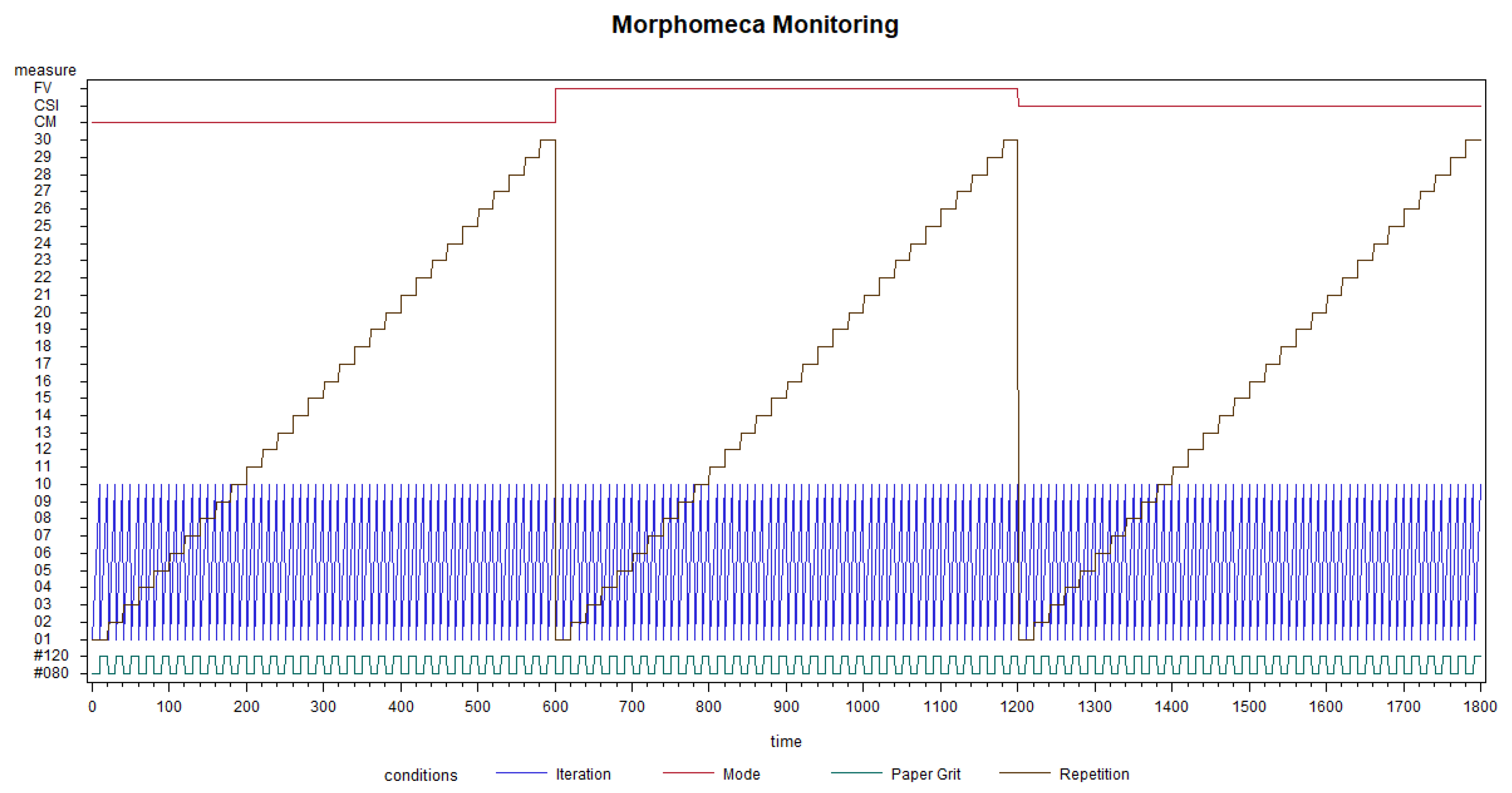
Figure 3. Organization of the measurement campaign (Morphomeca monitoring).

Figure 3. Organization of the measurement campaign (Morphomeca monitoring).

The chosen measurement strategy allows the quantification of influences of measurement conditions for the intercomparison of stitched measurements. Figure 3 shows the measurement plan including the three instrument modes (red line), the two grit papers (green line), the 30 repetitions (brown line), and the 10 iterations (blue line). From the iterations and repetitions, it becomes possible to characterize and quantify the quality, the drift and the stability of the instrument modes to finally find the most relevant instrument mode able to discriminate both grits #080 and #120. Each instrument mode performs 300 stitched measurements for each specimen (#080 and #120), including 30 repetitions (positions) themselves including 10 iterations. In total, 1800 (3 × 2 × 10 × 30) stitched measurements were performed on the two specimens.

Morphomeca monitoring is the visual representation of the measurement plan. Thanks to this representation, a quick comprehension is possible to make the parallel with the indexes. It is thus easy to have an idea of the weighting between the alternating of instruments, grits, iterations, and repetitions, and to know if the measurement plan is well-balanced.

2.3. The Four Indexes

The main objective of this paper is to know if a discrimination between two ground surfaces can be made for each mode. However, it is worth asking how to find the criteria of measurement characterization and how to quantify them.

Two aspects of measurement characterization can be identified [32]: the errors of measurement and the ability of an instrument to discriminate between two ground surfaces. To characterize the errors of measurement, three indexes are developed based on statistics: the quality index based on a signal-to-noise ratio, the drift index based on Durbin–Watson (DW) statistics, the stability index based on AutoRegressive (AR) models. A last index, the relevance index, based on ANOVA analysis, is used to quantify the ability to make a discrimination between the two ground surfaces (Figure 4).

The Sa intra-position represents the measurement variabilities in the iterations performed on each position (30 repetitions per surface) on the two ground surfaces. The Sa intra-position is computed by the bootstrap of Sa standard deviations, and obtained by random picking of 10 Sa values into series of iterations at each given repetition (position). Therefore, each randomly picked series of iteration has its own Sa standard deviation (30 values per surface). This bootstrap method is performed 10⁵ times on the 30 repetitions giving 3 × 10⁶ Sa standard deviation values per surface (see [32] for computational details).

The Sa inter-position represents the topographical variabilities between repetitions performed at each position (30 repetitions per surface) with 10 iterations (10 measurements at the same position) on the two ground surfaces. As the Sa intra-position, the Sa inter-position is computed by the bootstrap of Sa standard deviations and obtained by random picking of 30 Sa values into a given series of repetitions. In other words, the sets of Sa values are defined for each given iteration and made up of the 30 randomly picked repetitions (positions). Therefore, each randomly picked set of repetitions into a given iteration has its own Sa standard deviation (10 values per surface). This bootstrap method is performed 3 × 10⁵ times on the 10 iterations giving 3 × 10⁶ Sa standard deviation values per surface (to be compatible in size to the Sa intra-position standard deviation).

In a nutshell, two sets of 3 × 10⁶ Sa standard deviation values are generated: the first set represents the variation in Sa at a given position on a ground surface, and the other set represents the topographical variation between positions on the same ground surface.

The quality index (QI) represents the quality of the measurement, i.e., a signal-to-noise ratio between the signal represented by the Sa inter-position (the variation between the repetitions/positions) and the measurement noise represented by the Sa intra-position (the variation during iterations at given position). For the 3 × 10⁶ bootstrapped values, a ratio is computed between Sa inter- and intra-position to create histograms of QI values.

The drift index (DI) is computed from the Durbin–Watson (DW) test, itself computed from the iteration series. The DW test [33] can allow validation of whether a time auto-correlation exists between the Sa values into a series of iterations (between t and t − 1). The DW test returns a value between 0 and 4 with: 0 for a positive autocorrelation, 4 for a negative auto-correlation, and 2 for no autocorrelation. From these results, two p-values are computed in parallel on two hypotheses that are positive auto-correlation “not exist” and negative autocorrelation “not exist” noted, respectively: p-value-DW-negative and p-value-DW-positive. By comparison of the minimum of these two results, a p-values-DW is obtained called the DI. The hypothesis “not existing auto-correlation” is rejected when a DW value of 0.05 is obtained (DI = 0.025), giving the drifting threshold.

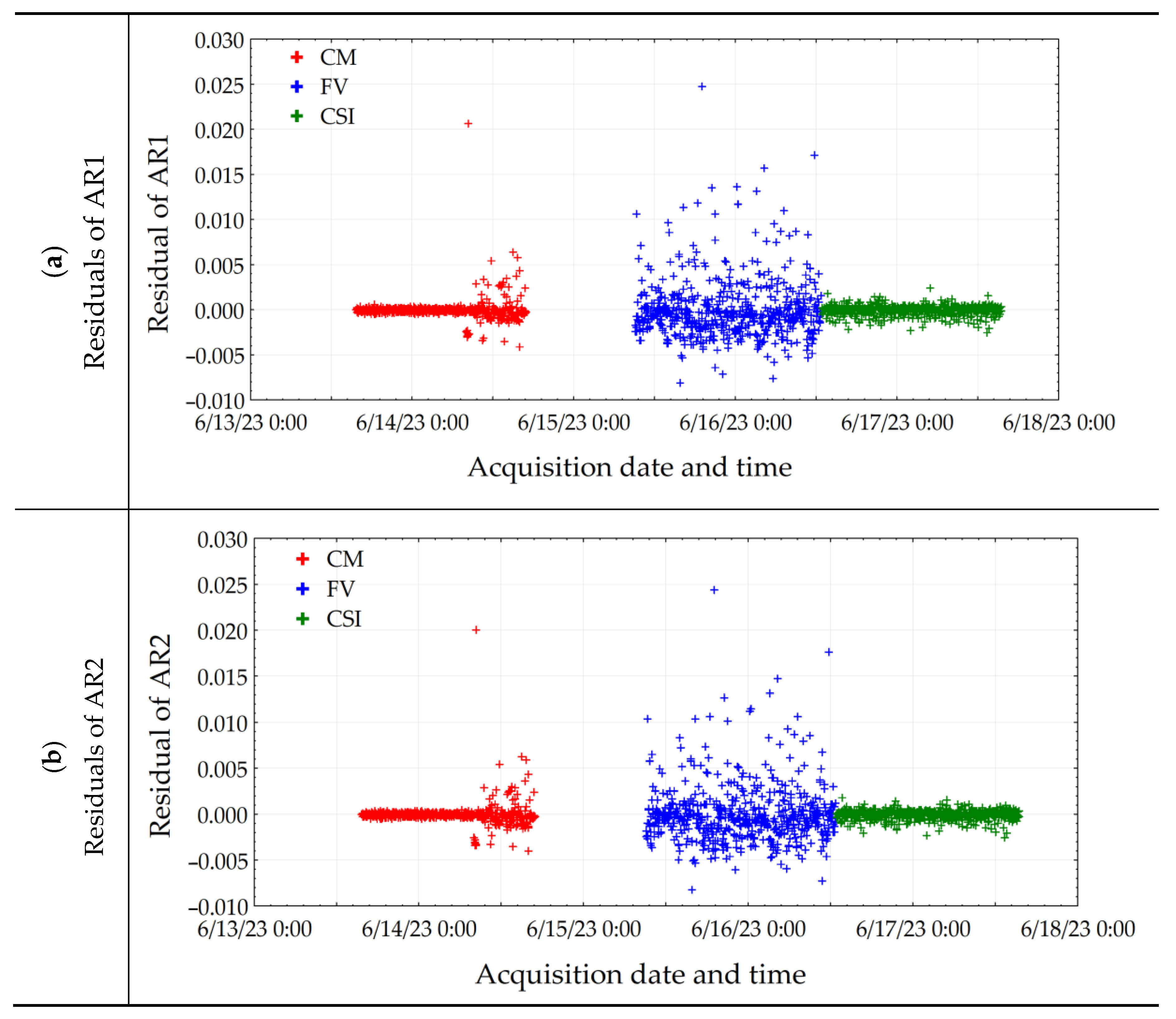
The stability index (SI) represents the ratio between the amplitude of the Sa values without drift and the total amplitude of the Sa values (raw Sa) into a series of iterations described in the Morphomeca monitoring. For each of these series, an autoregressive model is used to predict the Sa values and to calculate an associated residual. Two orders of autoregressive models [34] can be employed: order 1 (AR1), based on the current and one preceding Sa value of the series, and order 2 (AR2), based on the current and two preceding Sa values of the series (Appendix A). For each series of iterations, the difference between the real data series of Sa and the predicted values of Sa given by the AR model represents the residual. Regarding this given residual, AR2 describes slightly better the time evolution of the Sa values. A residual is also computing with the AR0 model (the raw data) representing the difference between the Sa values and the mean Sa of the iteration’s series. Therefore, SI represents the ratio of the variation between the residual of AR2 and the residual of AR0 (deviation from the average). In other words, SI gives a value between 0 and 1 corresponding to a level of prediction of the AR model. When the AR2 model is not able to predict the Sa values (${\mathsf{\epsilon }}_{\mathrm{A}\mathrm{R}\left(2\right)}\cong {\mathsf{\epsilon }}_{\mathrm{A}\mathrm{R}\left(0\right)}$), then SI tends to 1 because the noise is not correlated between measurements into a given iterations series. When the AR2 model is able to predict the Sa values (${\mathsf{\epsilon }}_{\mathrm{A}\mathrm{R}\left(2\right)}\cong 0$), then SI tends to 0 because it can describe a correlated noise into series. The SI threshold is defined to 0.5. The SI values superior to 0.5 are defined as stable and the SI values inferior to 0.5 are defined as unstable.

The stability is not directly an error but rather an indicator of the instrument behavior. Two indicators, called indexes, are able to describe the temporal behavior of the instruments. First, DI describes the local tendency between two iterations at a given position. It determines if a correlation does NOT exist whether it was positive or negative. On the other hand, SI determines the global law of the instrument temporal behavior with auto-regressive models to determine if the residuals are correlated or not. In a nutshell, DI gives local tendency of the temporal Sa fluctuation and SI gives a global model of this Sa temporal fluctuation.

A first relevance index (RI) is computed, based on ANOVA statistics, allows the assessment of the ability of the instruments to discriminate the two ground surfaces. ANOVA is used to compare the variance in Sa between the instruments with the variance in Sa within the instruments. If the variance in Sa between the instruments is significantly greater than the variance in Sa within the instruments, it is inferred that there are significant differences between the instrument means. ANOVA generates F-statistics expressing a ratio of inter-instrument Sa variance to intra-instrument Sa variance. It employs hypothesis tests to determine if the observed differences of the inter-instrument means are statistically significant.

A second relevance index is computed, also based on ANOVA, taking into account the main parameters: grits, instruments, and interaction of both (grit*instrument). It allows the assessment of the impact of the grits and the instruments on the roughness characterization.

3. Results and Discussion

3.1. The Raw Sa

The Sa values are plotted chronologically in Figure 5, and the three Sensofar instrument modes are represented in color: red for CM, blue for FV, and green for CSI. The two ground specimens measured are represented by markers: “+” for the #080 grit and “o” for the #120 grit. In Figure 5, each group of points surrounded by a cyan circle represents a series of iterations (10 measurements at a given position), and the population surrounded by an orange square represents a series of repetitions (30 measurement positions on a given specimen).

The Sa values are visually separated in two populations: grits #080 and #120. This means that the topographical signatures of the grinding process are clearly characterized through the Sa parameter according to the measurement conditions (stitching 6-by-7 and 20× magnification). The stitching area is large enough regarding the mean plan, the number of measured points, and the number of motifs to avoid Sa values mixing. Furthermore, the magnification gives a sufficient lateral resolution to describe the topographical motifs. But, on the chronological view of Sa, a break is made between the CM and FV instruments due to an unfortunate event in the control software constraint (corrected in a new release of the commercial software). However, it appears this break does not impact the measurements. The mean results of the Sa parameter are given in

Table 2. Mean values of Sa for the CM, FV, and CSI modes and for the grits #080 and #120.

Modes	CM		FV		CSI
Grit	#080	#120	#080	#120	#080	#120
Mean Sa (µm)	0.562	0.450	0.538	0.430	0.562	0.440
Increasing between #120 and #080 (%)	24.9		25.1		27.7

.

The difference in Sa values between grits appears visually 25.9% (+1.8%/−1%) higher for #080 compared to #120. In addition, it appears that the Sa values of the FV instrument (blue marks) are noisier between iterations than the CSI and CM instruments. It can also be observed that the measurement noise of the CM instrument (red marks) is not the same over the time. Indeed, the Sa dispersion during a given repetition is higher after 7.10 a.m. for the two ground surfaces. This may be due to the human activities which start at 7.10 a.m. in the premises where the measuring machine is located. Contrary to the CM mode, the FV and CSI instruments do not have an increase in dispersion during the time at first glance (from these primary results, investigations are in progress with the Sensofar company to reduce the human impact on the measurements).

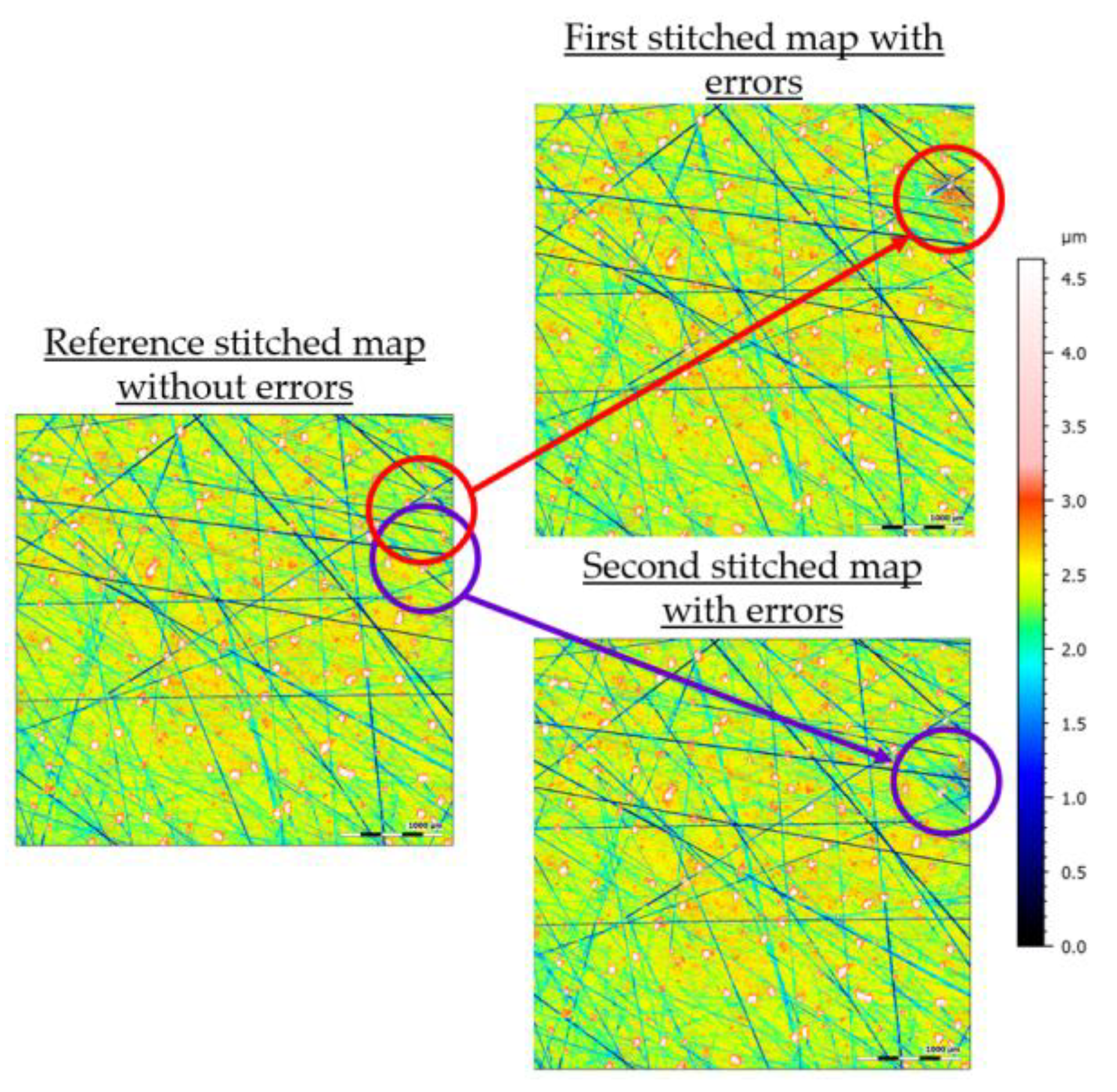
Figure 6 shows the stitched CM surface topographies in an iterations series after 7.10 a.m. having height fluctuations for two specific areas: the first map surrounded in red and the second map in purple. These local fluctuations do not concern isolated points but areas having the size of an elementary image, i.e., 839.7 × 701.7 µm. In addition, no stitching delimitations are observed in the stitched surfaces (pavement) which shows that a good stitching process is performed. A hypothesis is that a disturbance (external environment) occurred during the acquisition of these elementary maps and caused these fluctuations. The stitching algorithm therefore smoothed the deviations in order to construct the global map.

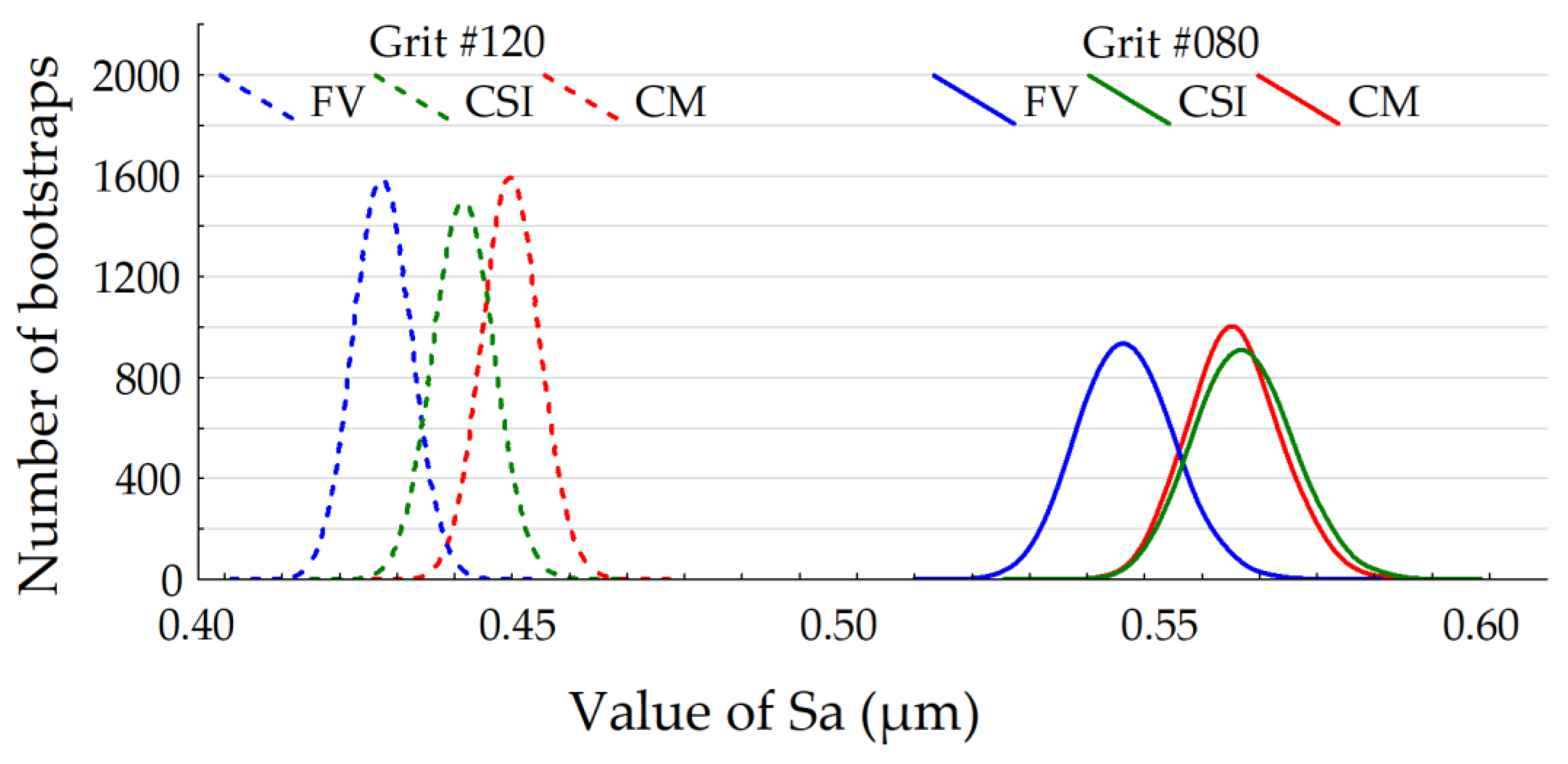
In Figure 7, the bootstrapped mean Sa values were plotted by instruments (CM, FV, and CSI) and by grits (#080 and #120). These Sa values are regrouped by class to create histograms. Globally, it is shown that Sa is lower for the grit #120 than the grit #080. As in Figure 5, it can be shown that the range of Sa is 25.9% higher in the case of #080 than #120. The normal aspect of histograms shows a homogeneous topographical variation (unimodal). The Sa distributions of the grit #080 are similar and are close to 0.56 µm. The Sa distributions of the grit #120 are different between the FV and CM instruments but CSI and CM are still near: the mean Sa is 0.45 µm for CM, 0.43 µm for FV, and 0.44 µm for CSI.

3.2. The Quality Index (QI)

3.2.1. Sa Intra-Position

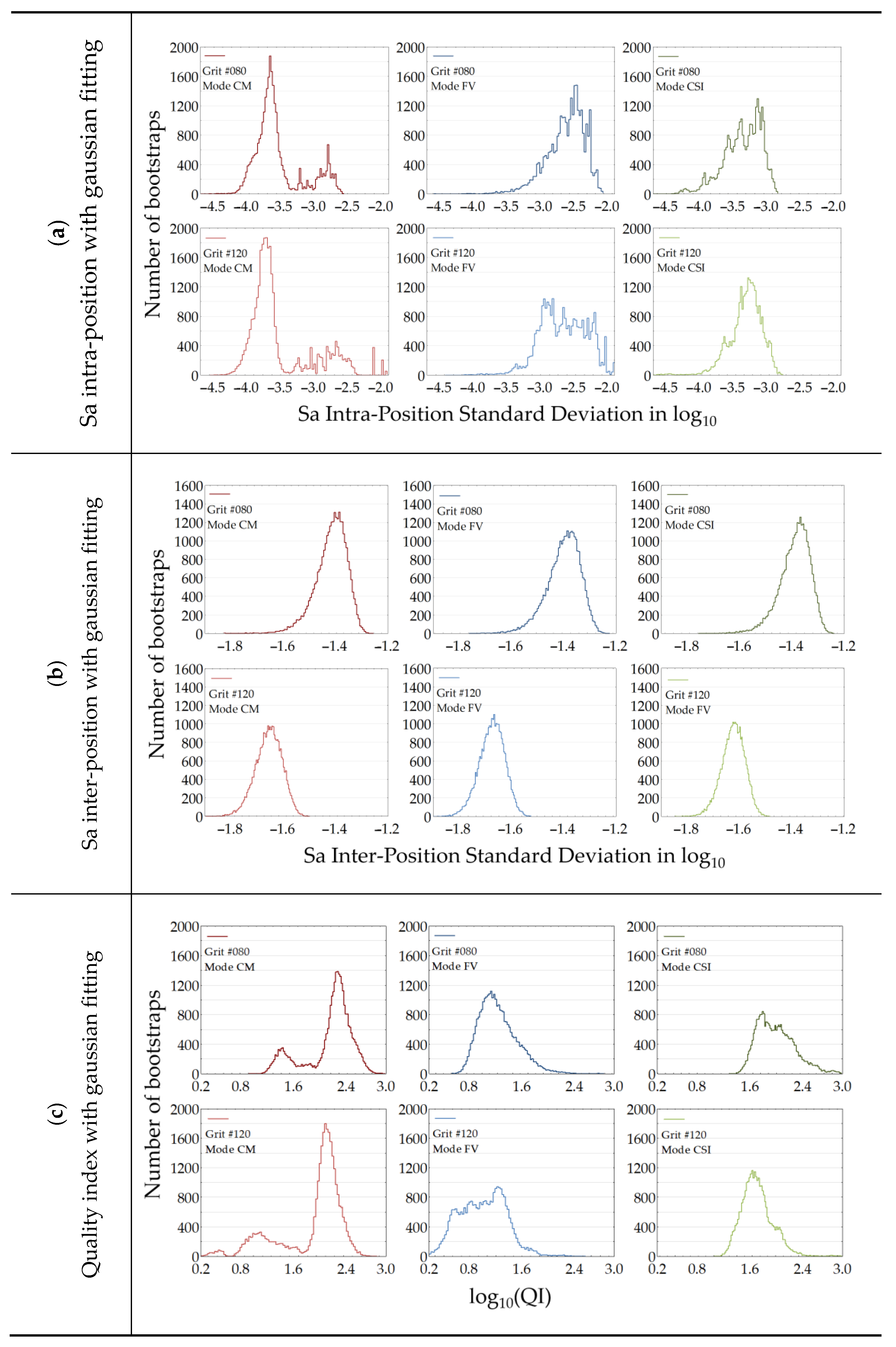
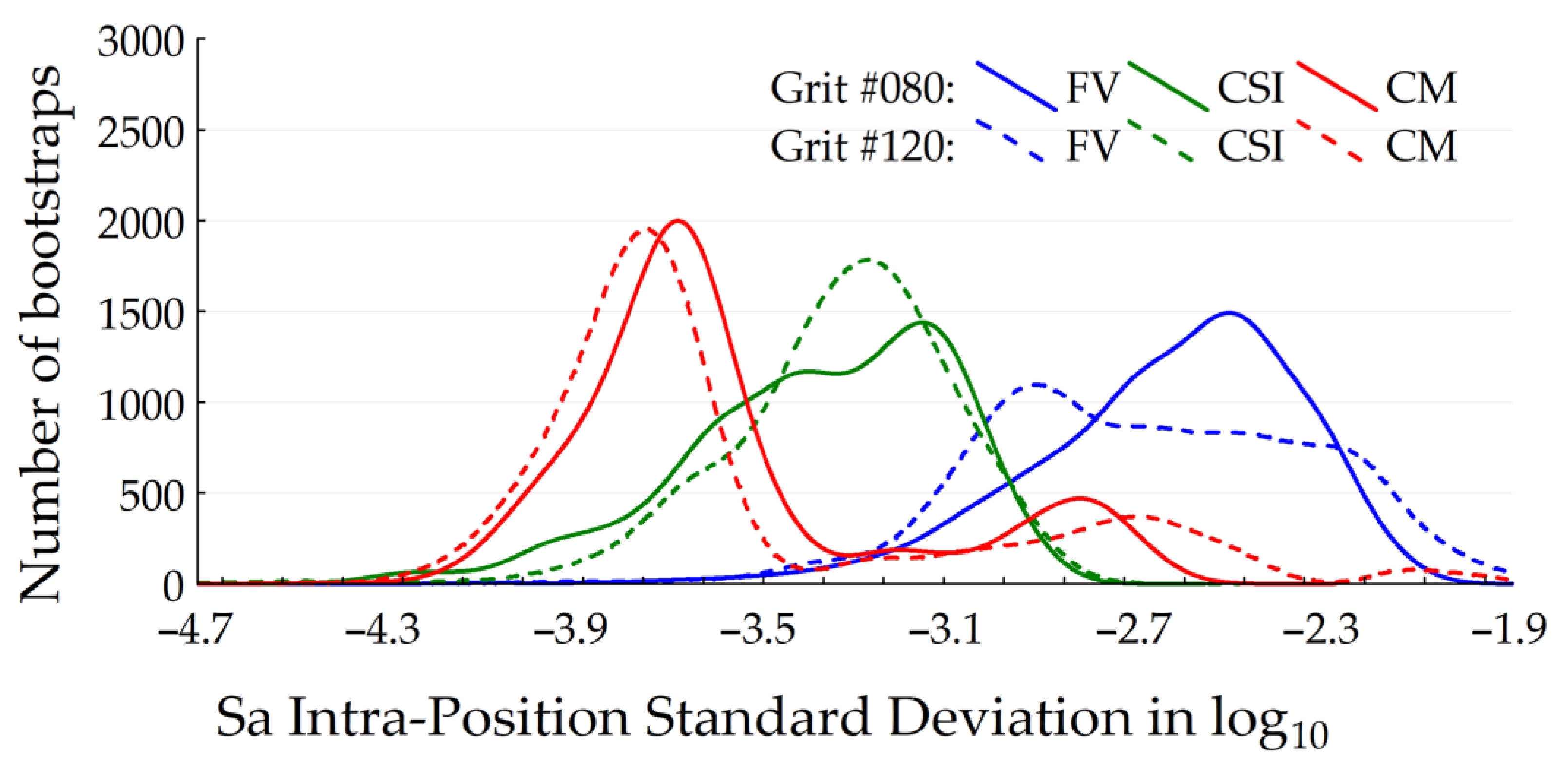
Figure 8 shows the bootstrapped Sa intra-position standard deviation values in log₁₀ plotted by instrument modes (CM, FV, and CSI) and by grits (#080 and #120). The measurement instruments are in color: red for CM, blue for FV, and green for the CSI instrument mode.

The histogram forms are relevant regarding the noise in the iteration series. The bootstrap method highlights the fact that the FV and CSI instrument modes have homogeneous histograms because their noise has a unimodal population. On the other hand, the CM instrument histograms have a bimodal population demonstrating that an event has disrupted the measurements. This hypothesis could be supported according to the observations made in Figure 5 showing the appearance of a measurement noise after 7.10 a.m. onwards. It could be noted that if the disruptive event had not occurred, the CM instrument would certainly be better than the other instrument modes, but this remains to be verified because of this disruption.

It is also interesting to highlight that the form of histograms is similar between the grits for the three measurement instrument modes. The measurement noise does not therefore depend on the grits but rather on the instrument modes. The CM instrument histograms have bimodal population, and have a wide range of values shared with the CSI mode. The FV instrument is more isolated from them.

As mentioned before, this index is able to highlight the Sa fluctuation at a given position. It is shown that the CM mode has a larger probability density function (PDF) than the other modes but has bimodal PDF due to an increase in the Sa fluctuation shown in Figure 5. If the fluctuation had not occurred, CM could have been the best mode regarding the principal mode at log₁₀ (Sa intra-position standard deviation = −3.8). It still appears to be the least stable (not the least qualitative) compared to the CSI and CM modes. The CSI mode has a not too large PDF compared to the other modes and is the second best regarding the Sa intra-position fluctuation. FV is the worst regarding the Sa intra-position fluctuation and is not too bad in stability.

3.2.2. Sa Inter-Position

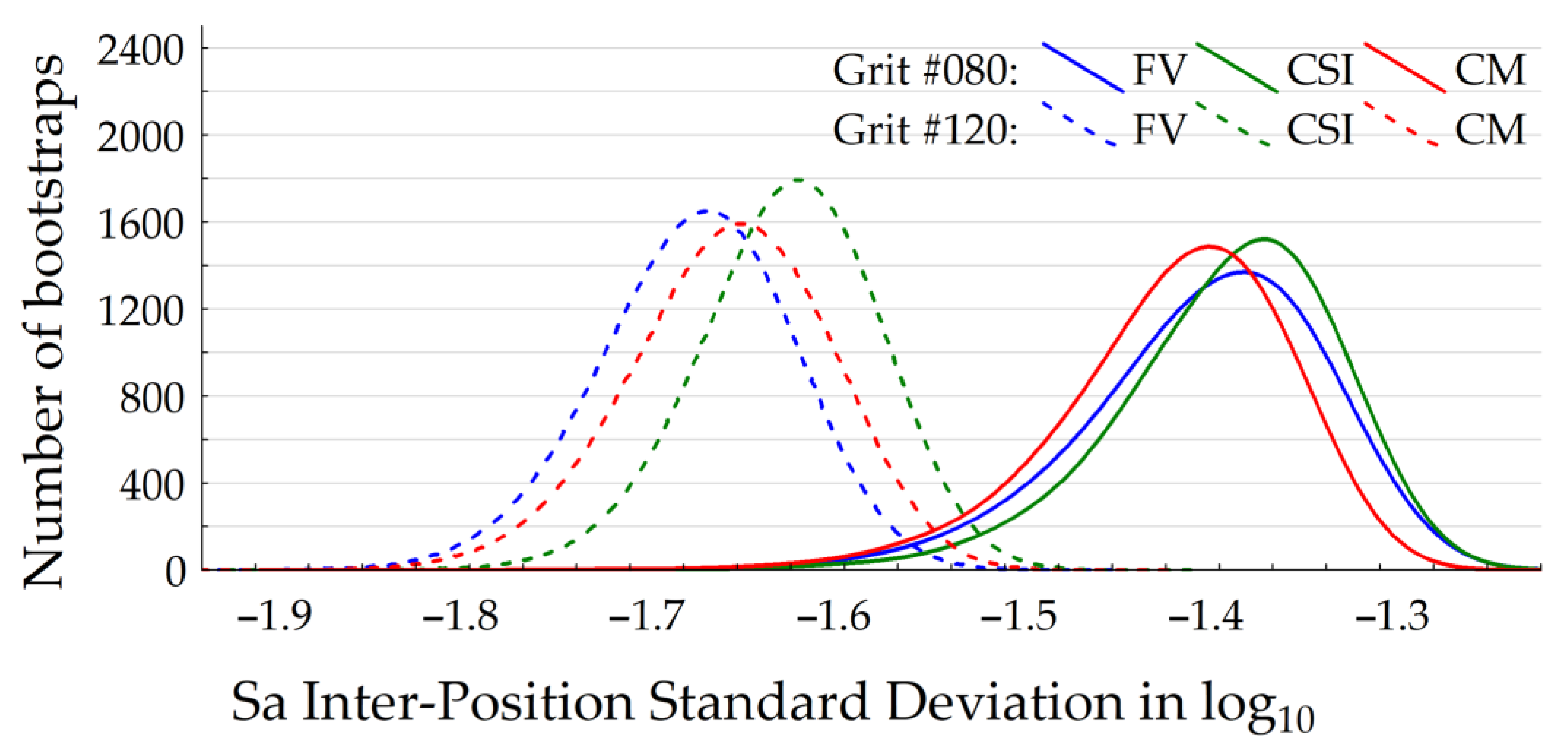
Figure 9 shows the bootstrapped Sa inter-position standard deviation values in log₁₀ plotted by measurement instrument modes (CM, FV, and CSI) and by grits (#080 and #120). The instrument modes are in color: red for the CM mode, blue for the FV instrument, and green for the CSI mode. The grits are represented by a solid line for the #080 and by a dotted line for #120.

All instruments have histograms with a normal form because their populations have homogeneous topographic variations. This means the process of grinding is under control, i.e., gives homogeneous surface topographies. In addition, each measurement instrument gives a close response at a given grit (#080 and #120) because the histograms are overlapped between instrument modes. This is why all instrument modes are thus able to measure topographical variations on given ground surfaces. But the Sa inter-position is more influenced by the grit than the measurement mode. This is evidenced because the topographical variations are led by the surface morphology.

The mean Sa inter-position standard deviation values are 0.040 µm for the grit #080 and 0.022 µm for the grit #120. This means that #080 has a dispersion twice (1.8) larger than #120. The amplitude of the surface topographies is higher for the grit #080 than the #120, and then the dispersion is more important for the grit #080. Moreover, the local slopes of surfaces are higher for the grit #080. It was shown the measurement uncertainties in optical devices increase with the local slopes of surfaces [35], and as a consequence, the Sa inter-position standard deviation values are higher for the grit #080.

3.2.3. Quality Index

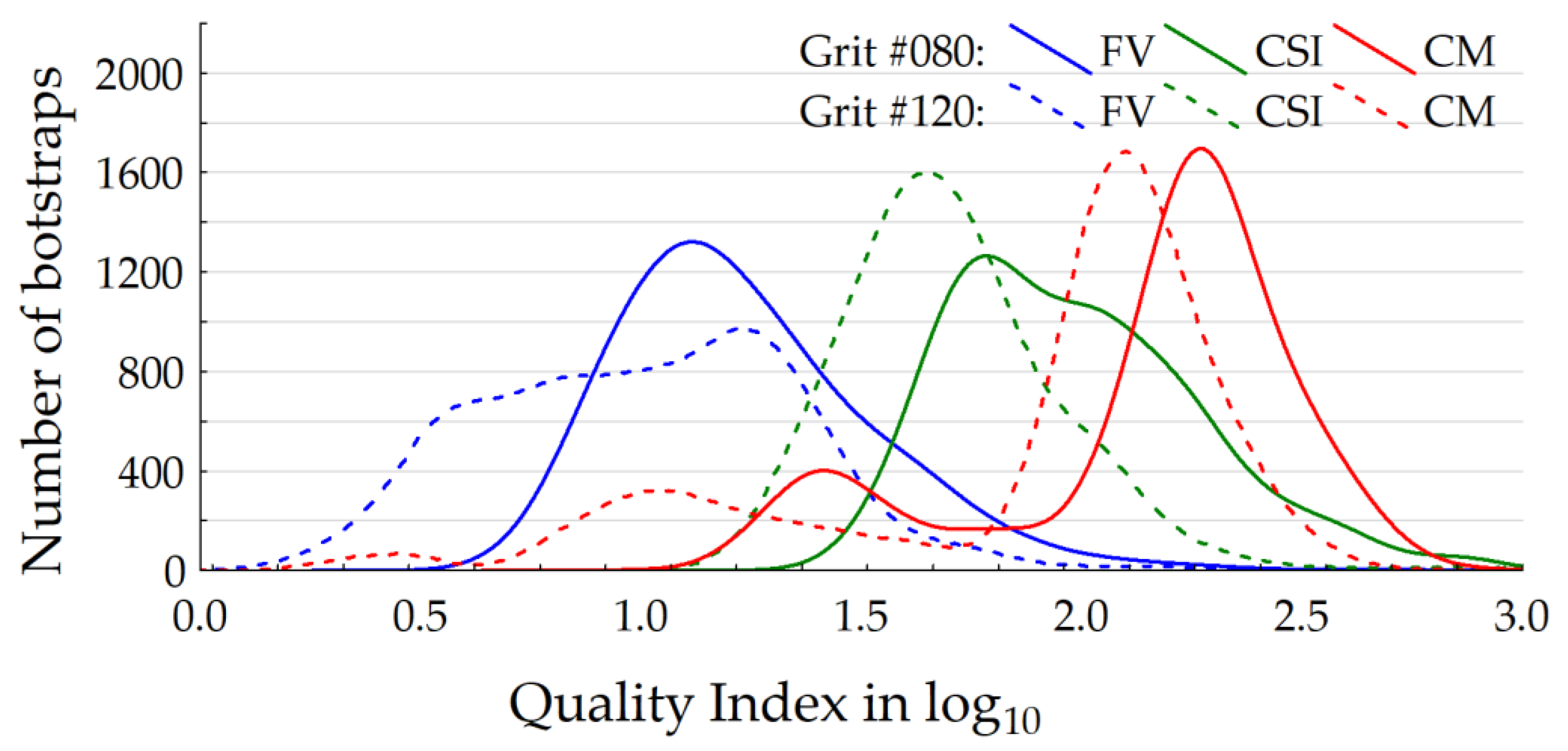
Figure 10 shows the quality index (QI) histograms in log₁₀ plotted by measurement instrument modes (CM, FV, and CSI) and by grits (#080 and #120). The instrument modes are in color: red for the CM mode, blue for the FV instrument, and green for the CSI mode. The grits are represented by a solid line for the #080 and by a dotted line for #120.

Despite the instability of the CM instrument shown in Figure 5, this instrument has higher QI values (QI = 180) than the CSI (QI = 56) and FV (QI = 14) instrument modes. On the other hand, the FV instrument has lower QI values with a higher dispersion of histograms. CSI has the most homogeneous histograms of QI with a lower dispersion. Globally, it can be shown that QI is better for the grit #080 than the grit #120. It can be explained by the fact that the topographical variation is higher for the grit #080 than the grit #120 (Sa inter-position depending on grit) and the noise (Sa intra-position) is mainly dependent on the instrument modes.

To conclude, QI is more dependent on the instrument than the grit because the histograms are more overlapped between the instrument modes. A summary of the Sa intra and inter-positions and QI is presented in Appendix B.

3.3. The Drift Index (DI)

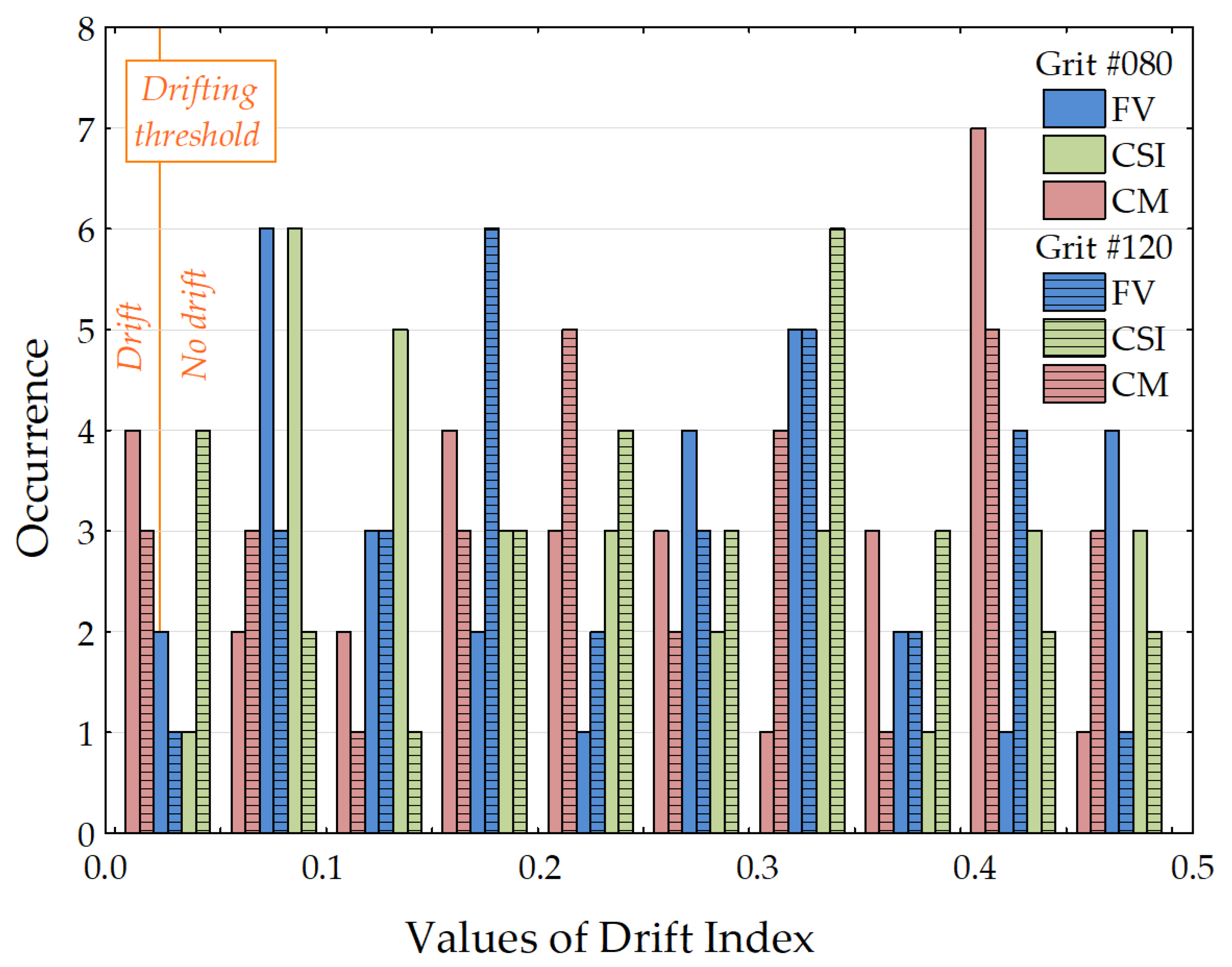
Figure 11 shows the drift index (DI) plotted by occurrence for the 180 series of iterations (180 measured positions for each grit and mode, i.e., 30 positions, 2 grits, and 3 instrument modes, and 10 iterations per measured position). The DI histograms are in color: red for the CM mode, blue for the FV instrument, and green for the CSI mode. The grits are represented by plain bars for #080 and by hatched bars for #120.

The more the DI (p-values-DW) tends to 0, the greater the autocorrelation (with a drifting critical value of 0.025). The histograms of DI are homogeneous overall because no grit or instrument mode is predominant for DI computed with the Sa values. All instrument modes and grits have no significative DI values, despite a variation in Sa during the iterations. Any instrument introduces drifting errors to the measurements.

3.4. The Stability Index (SI)

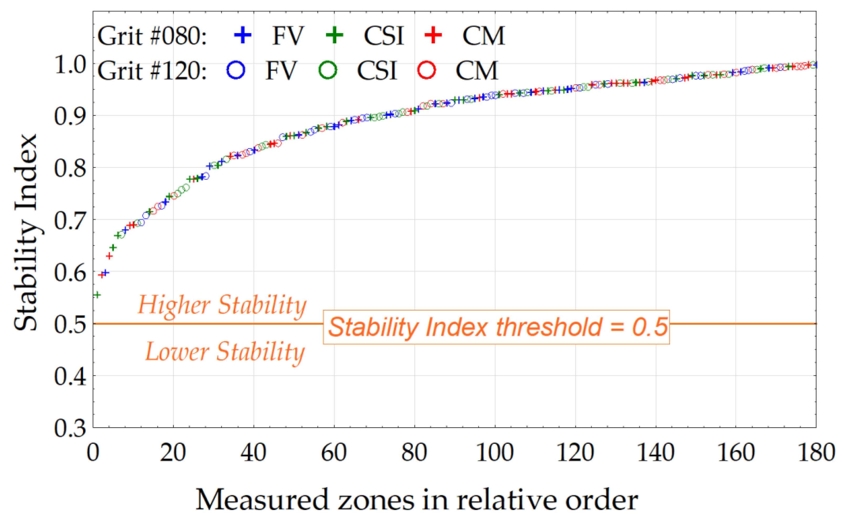
Figure 12 is an overall view of the stability index plotted by grits and measurement modes. The measurement modes are in color: the FV mode in blue, the CSI mode in green, and the CM mode in red, and the grits are represented by markers: “+” for #080 and “o” for #120. Each plotted value represents one series of iterations at a given position (180 positions in total, all grits and modes combined).

It is shown that the SI of the iteration series (180 values) is plotted in relative order. It is also shown that all series are above the threshold of 0.5 and no grit or mode is predominant near to 0.5, but it could be noted that the CM mode is slightly better for the values near to 1 and the majority of the SI values of the FV mode are in range from 0.85 to 0.95. The SI values of the CSI mode are not grouped and are more regularly represented in the curve.

But the number of points on stitched surfaces are significant and Sa is a roughness parameter describing an overall behavior, this is why the differences can be less pronounced.

3.5. The Relevance Index (RI)

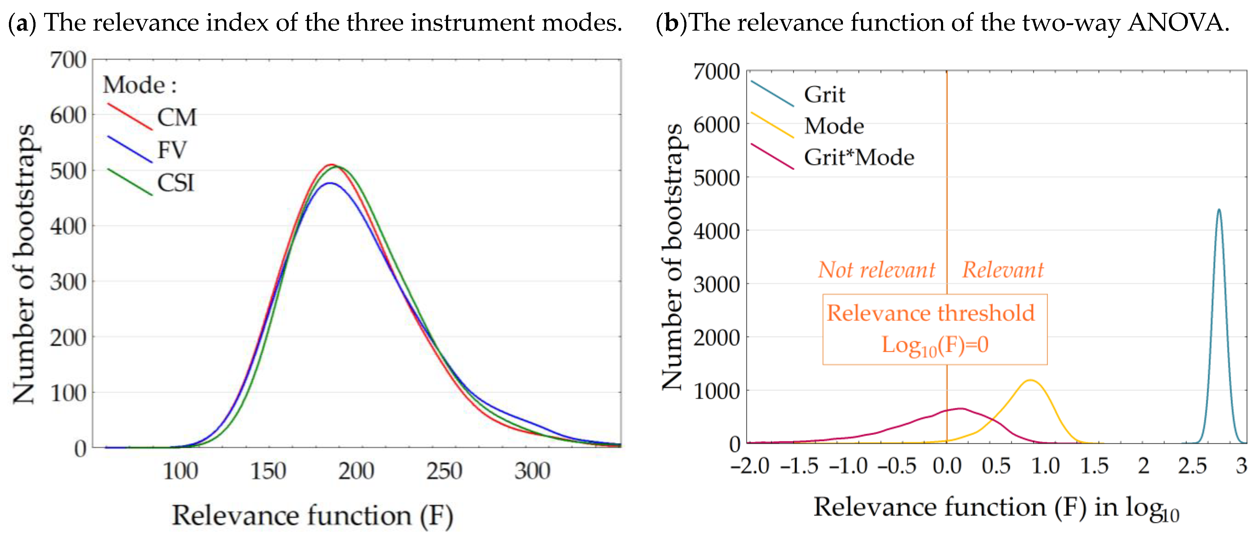
Figure 13 shows the relevance index (RI) of the three S neox™ measurement modes and based on the Sa parameter. The modes are discriminated by color: the CM mode in red, the FV mode in blue, and the CSI mode in green. The RI distribution based on ANOVA analysis shows that all modes are able to discriminate both grits #080 and #120 with the same ease. As F is significantly larger than 1, it clearly means that all instrument modes discriminate the two grits. Moreover, the histograms are totally overlayed, meaning that the instruments discriminate the ground surfaces in exactly the same way.

Figure 13 shows the two-parameters relevance function of two-way ANOVA with interaction on the Sa parameter between the grits in blue, the modes in yellow, and the interaction between both (grit*mode) in purple. The relevance threshold of the function is set to 1 corresponding to log₁₀(F) = 0 (no impact, no influence if F ≤ 1, i.e., log₁₀(F) ≤ 0). It clearly appears that the combined effect between the grits and the modes (grit*mode) has no impact on the measurement system results (no significant interaction). The instrument is the significant parameter (F = 5 > 1, i.e., log₁₀(F) = 0.7 > 0). This means that the instruments give different Sa values. The grit is the most significant parameter (F = 795 >> 1, i.e., log₁₀(F) = 2.9 >> 0). This clearly indicates that the multi-instrument measurement system distinguishes the ground surfaces (grit effect) regardless of the used mode and with the same quality of discrimination. As there is no interaction effect, we conclude that, regardless of the measurement system, the topographical differences (characterized by the Sa roughness parameter) are statistically identical.

3.6. Assessment of Differences between Stitched and Elementary Measurement

According to a previous work [32], a comparison is made between stitched and elementary measurement for the Sa intra-position, the Sa inter-position, and the QI index. It was decided to highlight how the stitched measurements influence these indexes. It is necessary to specify that the measurement plan carried out in the case of the elementary surface campaign are slightly different. Indeed, as shown in [32], the measurement plan alternates #080 and #120 at each measurement unlike the measurements of this paper, where the stitched measurements are performed 10 times at a given position before changing position. But these results can be comparable anyway because the repositioning operations are made between each stitched measurement as between each elementary measurement in the other campaign.

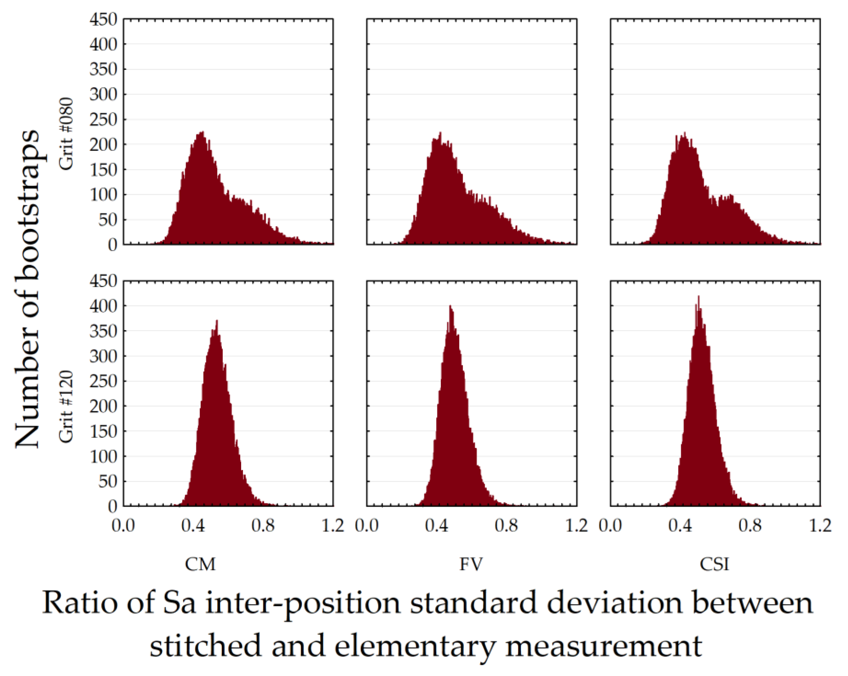
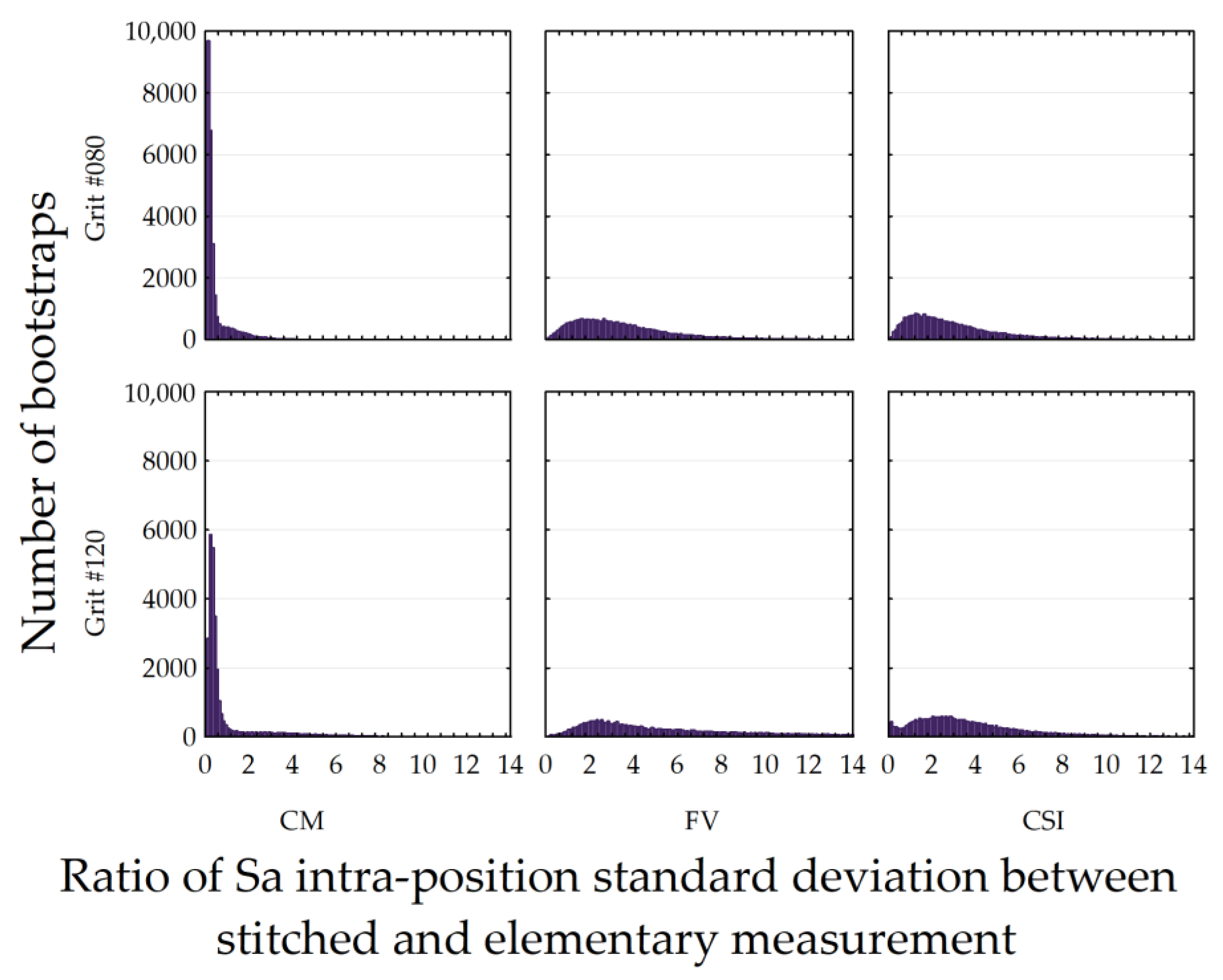
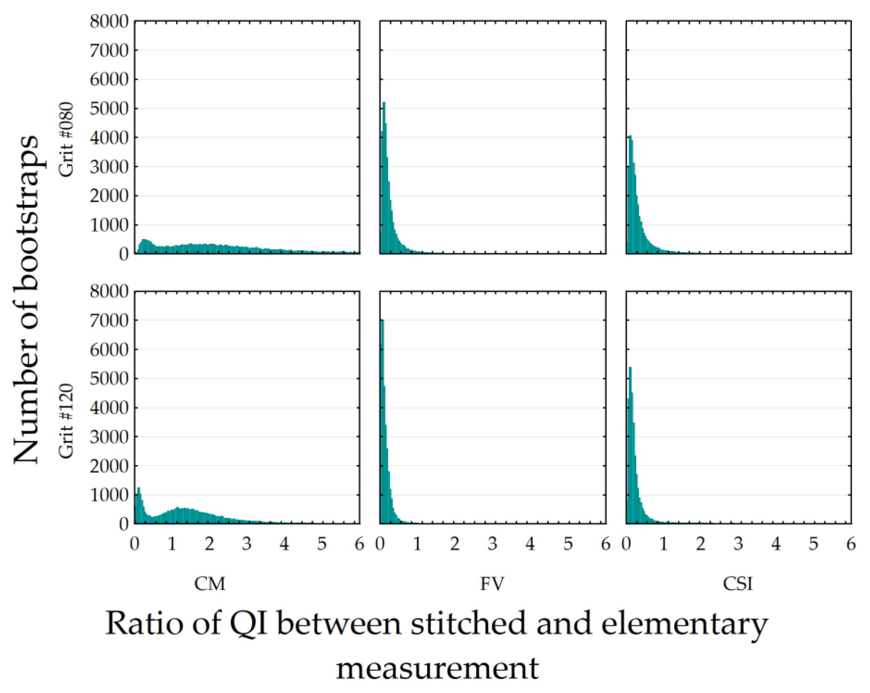
To compare the elementary and stitched measurement, a ratio is computed between their probability densities, respectively, for the Sa intra-position standard deviation (Figure 14), the Sa inter-position (Figure 15), and the QI index (Figure 16). It is shown that the Sa inter-position standard deviation is twice as low on the stitched surfaces as on the individual measurements, regardless of the measurement method used (CM, FV, or CSI). This trend does not seem to depend on the nature of the sample grinding. This finding becomes even more interesting when considering that the stitched surfaces combine 42 individual surfaces, resulting from the combination of a 6 × 7 matrix. By grouping these surfaces in this way, the roughness value Sa becomes more representative, and consequently, the data dispersion decreases. Additionally, the reference plane becomes better defined, further contributing to the reduction in the measurement dispersion.

It is also remarkable that this convergence towards a unique value (i.e., 0.5) could suggest that we have approached the true topographic variability of the grinding process, regardless of the measurement system used. This observation highlights the crucial importance of the combined measurement techniques and stitched data analysis to obtain a more precise and representative understanding of the ground surface topographies.

However, the ratio of intra-position standard deviations is higher for the stitched topographies than for the individual topographies (

Table 3. Summary of the ratio values of the Sa intra/inter-position standard deviations and QI for CM, FV, and CSI, and grits #080/#120.

	CM		FV		CSI
Grit	#080	#120	#080	#120	#080	#120
R(intra)	0.48	1.33	3.49	6.20	2.98	2.93
R(inter)	0.52	0.53	0.51	0.50	0.51	0.52
R(Q)	1.78	1.29	0.25	0.14	0.31	0.27

). This cannot be attributed to the repositioning errors since the sample is moved for each individual measurement, i.e., successive measurements on #080, then #120. This is certainly due to the stitching algorithms which may introduce overlapping errors, thus introducing an additional source of topographic variability, particularly in the blending zone.

Concerning the quality index, the ratio between the measurement quality depends on the instruments. For the CM mode, the ratio is greater than 1 (1.5), indicating that this mode is more precise for the stitching mode than the individual mode. However, the CSI mode shows a lower quality ratio for the stitching mode (0.29), and FV has an even lower quality ratio (0.2). Nevertheless, it is shown that the quality ratio is lower for the grit #120 than the grit #080. A possible explanation is that the roughness peaks, particularly the scratches, have a higher amplitude and width, which could reduce repositioning errors.

4. Conclusions

In our comprehensive study, we have implemented a metrological methodology, known as Morphomeca monitoring, for the scheduling and analysis of topographical measurements. This multi-parameter approach integrates four distinct interrelated indexes: repeatability (quality index), stability (stability index), drift (drift index), and relevance (relevance index), allowing the quantification of the quality and reliability of measurements. The outcomes of our investigation highlight several observations:

• The examination reveals a notable absence of measurement drift within the system. This implies that both the stitching methodology and repositioning process are meticulously controlled for all three technologies, i.e., interferometry, confocal microscopy, and focus variation.
• The measurements show a high level of stability. This signifies that the repositioning aspect remains consistently unaffected over time for all three instrument modes.
• A nuanced analysis indicates that the quality of measurements is contingent upon the chosen metrology. Specifically, interferometric microscopy emerges as the most robust, followed by confocal microscopy, then focus variation microscopy. A preliminary investigation suggests that the quality of stitching plays an essential role and is inherently linked to the chosen measurement technique. Despite variations in the measurement quality for the three instrument modes, the robustness remains a constant for each grit, thereby minimizing the potential introduction of interpretation biases. Intriguingly, the bootstrap analysis brings to light a time-dependent aspect of robustness for the confocal mode, potentially associated with human presence during measurements.
• Notably, despite the low ability to discriminate some particular surface motifs, the Sa roughness parameter discriminates the two grits accurately. This underscores the reliability and effectiveness of the proposed metrological methodology.

Therefore, the proposed methodology can be aptly characterized as:

• Robust: demonstrating resilience and consistency across different conditions and methodologies.
• Reproducible: yielding consistent results upon repeated measurements.
• Automatable: exhibiting the potential for automation, thereby enhancing efficiency.
• Data monitoring as a diagnostic tool: highlighting the significance of data monitoring as an invaluable tool for identifying and addressing metrological challenges.

It is imperative to note that our focus has primarily been on the Sa roughness parameter without multi-scale treatment. The comprehensive treatment of all other relevant parameters has been undertaken, paving the way for future investigations such as the classification of indexes based on specific roughness parameters for each device. A forthcoming analysis promises to provide a detailed metrological characterization of responses concerning amplitude, frequency, shape, gradient, curvature, patterns, and more. By including these parameters, the future study will allow capturing aspects of topography that are not fully represented by a single parameter such as Sa (average roughness).