Impact of Angular Speed Calculation Methods from Encoder Measurements on the Test Uncertainty of Electric Motor Efficiency

Abstract

The imperative need to advance the development of more efficient electric motors requires the meticulous measurement of small increments while minimizing the associated uncertainty in dynamometer tests. One of the key variables in such tests is the angular speed, which is typically obtained based on encoder measurements. This paper proposes a systematic measurement uncertainty assessment method based on the Guide to the Expression of Uncertainty for the two most widely used methods for angular speed measurement, namely, the frequency and period methods. In addition, the impact of the angular speed calculation method on the efficiency test uncertainty is assessed using an automatic test rig for electric motors. Our experimental results consider both steady-state and dynamic analyses. The results show that the period measurement method provides measurements with lower uncertainty for the encoders typically used in such test rigs, about 30 times less than the uncertainty determined for the frequency measurement method. Based on these results, the choice of a proper method can drastically decrease the angular speed uncertainty, and consequently the motor efficiency uncertainty, without increasing instrumentation cost.

1. Introduction

Due to rising concerns around the increasing demand and limited availability of energetic resources, recent decades have seen a trend towards product design strategies which prioritize increased efficiency [1]. A particularly important segment of this design trend is the research and development of electrical drives [2,3]. Thanks to these improvements, the highest efficiency classes of modern electric motor standards can reach over 95% efficiency [4], with many research topics still ongoing [1].

Considering the long history and wide span of electric motor applications, current research is mostly driven by small improvements over well established models [1,5]. In such cases, operating and analyzing motors in the high-efficiency region requires accurate measurements for both losses and power output, which are used to evaluate the efficiency of the system [6,7]. Measurement system uncertainty is also a concern when dealing with product standardization, as efficiency tests must be performed with the lowest uncertainty possible in order to allow for correct classification of the efficiency classes defined in local and global standards [3].

The evaluation of the real-world capabilities of motors is usually performed under dynamometer testing, which applies different loading conditions at different angular speeds. The power output of the motor, which is the prime object of these tests, is derived from torque and angular speed, the latter of which can be estimated based on the angular displacement of the motor shaft. This estimation allows for the use of cost-effective alternatives such as encoders [8], as the limitations posed by low-resolution encoders can be mitigated to an extent by choosing an appropriate angular speed calculation or estimation algorithm. The estimation itself can be performed in several ways depending upon the accuracy and bandwidth needed for the particular application, processing capabilities of the microcontroller or programmable logic controller used for implementation, and considerations around system cost and complexity, which often involve significant trade-offs [9,10,11].

Among the many methods proposed in the literature for estimating angular speed based on incremental encoders, two are considered to be fundamental: the frequency measurement method, in which the angular speed is estimated according to the number of encoder pulses in a given time window, and the period measurement method, in which the angular speed is estimated based on the period between consecutive encoder pulses [12]. These methods are well established in industry, and the more sophisticated estimation methods in the literature mostly rely on these concepts as their cores while improving precision and performance by of combining both approaches or including filtering techniques in the estimation process [10,13,14,15].

While there are publications which have explored factors such as computational cost and the feasibility of estimation methods in different applications [12,15], the literature on the subject lacks a proper examination of the implications of method choice on the assessed uncertainty in motor tests. Considering the high precision required for efficient research testing, the metrological aspects of each method are a key factor for ensuring reliable results; yet, they remain under-researched.

The aim of this study is to investigate the impact of angular speed calculation methods on the uncertainty of motor efficiency tests. For this purpose, an automatic test rig was employed to measure quantities needed to calculate electric motor efficiency. Two angular speed calculation methods were tested simultaneously, with the individual and final uncertainties assessed according to the Guide to the Expression of Uncertainty of Measurement (GUM) [16]. The results, presented across different angular speeds, should be taken into account when designing high-efficiency motor tests which include incremental encoders, and can also serve as a guideline for reducing uncertainty in test rigs without increasing instrumentation cost.

The rest of this work is organized as follows. Section 2 presents the angular speed calculation methods studied in this paper. Section 3 describes the uncertainty analysis regarding each of the speed calculation methods used in different scenarios. Section 4 presents the test rig employed for data acquisition. Section 5 describes the experimental study, highlighting the behavior of the methods on both steady-state and dynamic measurements. Section 6 discusses the impacts of each angular speed method’s uncertainty on the motor efficiency. Finally, Section 7 presents the conclusions of this paper, along with an assessment of the benefits and limitations of each method.

2. Angular Speed Calculation Methods

This section introduces two angular speed calculation methods: the frequency measurement method and the period measurement method. The primary equations governing the behavior of these methods are systematically presented, accompanied by explanations of their distinctive characteristics.

2.1. Frequency Measurement

The conventional and most straightforward approach for quantifying the rotor angular speed involves directly assessing the frequency of encoder pulses. This method consists in counting the quantity of detected pulses within a fixed and consistent time interval. Subsequently, the angular speed is estimated by employing discrete incremental ratios, assuming a uniform angular speed within the observation windows. This calculation is expressed as follows:

$${\omega }_{\mathrm{f}}=\frac{\Delta N}{t_{\mathrm{w}}{N}_{\mathrm{p}}},$$

(1)

where ${\omega }_{\mathrm{f}}$ is the angular speed calculated using the frequency method, $\Delta N$ is the number of encoder pulses during the acquisition time window $t_{\mathrm{w}}$, and $N_{\mathrm{p}}$ is the number of pulses per revolution of the encoder.

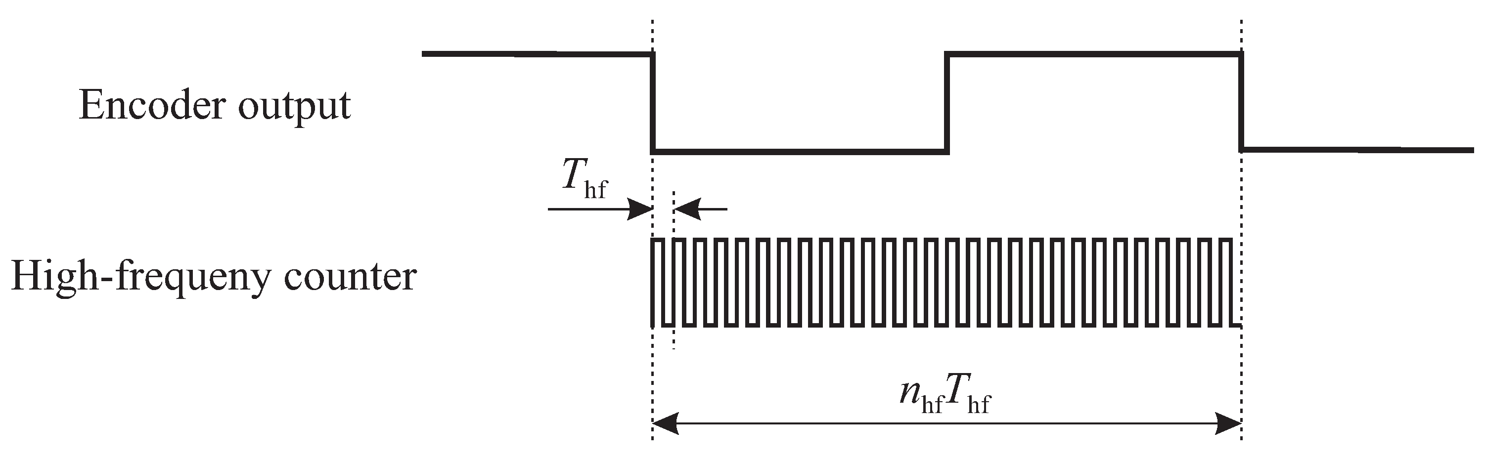
2.2. Period Measurement

An alternative approach to that presented in Section 2.1 is the period measurement method, in which measurement is accomplished by counting the number of cycles of a high-frequency signal contained within a single or multiple successive encoder pulses, as illustrated in Figure 1.

The subsequent equation is derived under the assumption that the angular speed remains constant, and only a single period of the encoder signal is taken into account:

$${\omega }_{\mathrm{p}}=\frac{1}{N_{\mathrm{p}}{n}_{\mathrm{hf}}{T}_{\mathrm{hf}}},$$

(2)

where ${\omega }_{\mathrm{p}}$ is the angular speed calculated using the period method, $n_{\mathrm{hf}}$ is the number of high-frequency pulses observed, and $T_{\mathrm{hf}}$ is the high-frequency pulse period.

3. Uncertainty Analysis of the Angular Speed Calculation Methods

This section delves into quantifying and comprehending the uncertainties inherent in the frequency measurement and period measurement methods presented in Section 2. The assessment of such uncertainties directly impacts the final uncertainty of the motor efficiency test.

Assessment of the propagation of uncertainty between the components and quantities follows the law of propagation of uncertainties [16], provided by

$${u_{\mathrm{c}}}^2\left(y\right)=\sum _{i=1}^N{\left(\frac{\partial y}{\partial x_i}u\left(x_i\right)\right)}^2,$$

(3)

where ${u_{\mathrm{c}}}^2\left(y\right)$ is the combined standard uncertainty, $u\left(x_i\right)$ is the standard uncertainty of the input quantity $x_i$, and $\frac{\partial y}{\partial x_i}$ is the sensitivity coefficient.

3.1. Frequency Measurement

For the frequency measurement method, the following uncertainty components have been considered:

• $u_1\left({\omega }_{\mathrm{f}}\right)$: repeatability
• $u_2\left({\omega }_{\mathrm{f}}\right)$: method resolution
• $u_3\left({\omega }_{\mathrm{f}}\right)$: time base variability
• $u_4\left({\omega }_{\mathrm{f}}\right)$: non-uniformity of encoder markings

For the repeatability of the mean of the measurements, a Type A component based on the standard deviation of measurement data was used to estimate the uncertainty. For the motor efficiency testing, because the measurements are taken over a defined period in which the electrical motor is operating on a certain condition, the interest lies over the variables means in consecutive measurements. This part is calculated as follows:

$$u_1\left({\omega }_{\mathrm{f}}\right)=\frac{{\omega }_{\sigma }}{\sqrt{n}},$$

(4)

where ${\omega }_{\sigma }$ is the standard deviation for the $\omega$ measurement and n is the number of measurement repetitions.

The second uncertainty component, $u_2\left({\omega }_{\mathrm{f}}\right)$, is calculated using the method resolution. Because $\Delta N$ is a non-null natural number, an uncertainty component emerges as an additional factor influencing the actual average angular speed within the observation window, provided by:

$$u_2\left({\omega }_{\mathrm{f}}\right)=\frac{1}{t_{\mathrm{w}}{N}_{\mathrm{p}}}.$$

(5)

This uncertainty component is contingent upon the variability associated with the measured pulse count $\Delta N$, arising from the lack of synchronization between encoder pulses and the observation window timing. This results in a $u_2\left({\omega }_{\mathrm{f}}\right)$ dependent upon the encoder characteristics, which can be balanced by choosing the appropriate acquisition time window. This behavior is shown in Figure 2.

In Figure 2, the parameter $N_{\mathrm{p}}$ changes between 30 pulses and 360 pulses, while $t_{\mathrm{w}}$ is in the range between 50 $\mathrm{m}$$\mathrm{s}$ and 500 $\mathrm{m}$$\mathrm{s}$. Considering a low-resolution encoder, if the observation window is short, then the uncertainty presented in (5) tends to increase drastically. To balance this, the observation window must increase in order to reduce $u_2\left({\omega }_{\mathrm{f}}\right)$, with the drawback of reducing the controller bandwidth. This method is not suitable for characterizing instantaneous angular speed variations, as only the mean angular speed is acquired every $t_{\mathrm{w}}$. This can be an issue for use in a dynamometer test, as loads can be unbalanced and measurement of the angular speed fluctuation is important in certain analyses.

The third uncertainty component, $u_3\left({\omega }_{\mathrm{f}}\right)$, relies on the timing uncertainty specifications for the data acquisition (DAQ) board, which directly impacts the value of $t_{\mathrm{w}}$ in (1). The parameter $t_{\mathrm{w}}$ is assumed to be known and constant, although it has some inherent uncertainty $u\left(t_{\mathrm{w}}\right)$. This uncertainty component is obtained by taking the derivative of ${\omega }_{\mathrm{f}}$ in (1) with respect to $t_{\mathrm{w}}$ in order to obtain the sensitivity coefficient, provided by

$$\begin{array}{cc}\hfill \frac{\partial {\omega }_{\mathrm{f}}}{\partial t_{\mathrm{w}}}& =-\frac{\Delta N}{{t_{\mathrm{w}}}^2{N}_{\mathrm{p}}}\hfill \\ \hfill & =-\frac{{\omega }_{\mathrm{f}}}{t_{\mathrm{w}}},\hfill \end{array}$$

(6)

then multiplying it by the uncertainty regarding $t_{\mathrm{w}}$, resulting in

$$u_3\left({\omega }_{\mathrm{f}}\right)=-\frac{{\omega }_{\mathrm{f}}}{t_{\mathrm{w}}}u\left(t_{\mathrm{w}}\right),$$

(7)

where $u\left(t_{\mathrm{w}}\right)$ is the timing resolution uncertainty of the measurement device.

The fourth uncertainty component, $u_4\left({\omega }_{\mathrm{f}}\right)$, is related to constructive issues regarding the encoder markings, resulting in non-uniform allocation of pulses within a shaft revolution. When using the frequency method, $\Delta N$ can suffer a variation caused by the first and last pulses, which can cause the identification a different number of pulses, directly impacting (1). Thus, the $u_4\left({\omega }_{\mathrm{f}}\right)$ component can be obtained by taking the derivative of ${\omega }_{\mathrm{f}}$ in (1) with respect to $\Delta N$, provided by

$$\begin{array}{cc}\hfill \frac{\partial {\omega }_{\mathrm{f}}}{\partial \Delta N}& =\frac{1}{t_{\mathrm{w}}{N}_{\mathrm{p}}}\hfill \\ \hfill & =\frac{{\omega }_{\mathrm{f}}}{\Delta N},\hfill \end{array}$$

(8)

and multiplying by the uncertainty regarding $\Delta N$, which in this case is provided by the relative deviation of the encoder markings. Because only the first and last markings acquired are relevant for this method and their effects are independent from each other, the square root of the sum of squares for both markings is considered, and the uncertainty is provided by

$$\begin{array}{cc}\hfill u_4\left({\omega }_{\mathrm{f}}\right)& =\sqrt{{\left(\frac{{\omega }_{\mathrm{f}}}{\Delta N}\frac{{\sigma }_{\mathrm{m}}}{{\mu }_{\mathrm{m}}}\right)}^2+{\left(\frac{{\omega }_{\mathrm{f}}}{\Delta N}\frac{{\sigma }_{\mathrm{m}}}{{\mu }_{\mathrm{m}}}\right)}^2}\hfill \\ \hfill & =\sqrt{2}\left(\frac{{\omega }_{\mathrm{f}}}{\Delta N}\frac{{\sigma }_{\mathrm{m}}}{{\mu }_{\mathrm{m}}}\right),\hfill \end{array}$$

(9)

where ${\sigma }_{\mathrm{m}}$ is the standard deviation of the encoder markings and ${\mu }_{\mathrm{m}}$ is the mean encoder marking size.

3.2. Period Measurement

For the period measurement method, the following uncertainty components have been considered:

• $u_1\left({\omega }_{\mathrm{p}}\right)$: repeatability
• $u_2\left({\omega }_{\mathrm{p}}\right)$: method resolution
• $u_3\left({\omega }_{\mathrm{p}}\right)$: timing resolution of the DAQ
• $u_4\left({\omega }_{\mathrm{p}}\right)$: non-uniformity of encoder markings

Similar to Section 3.1, $u_1\left({\omega }_{\mathrm{p}}\right)$ is calculated using (4). For the sake of clarity, the deduction of the resolution of the method related to $u_2\left({\omega }_{\mathrm{p}}\right)$ is based on the perspective that the period measurement relies on the sampling time instead of using a high-frequency counter. Similar to (1), where the angular speed is calculated based on the number of pulses detected during a time window, the calculation of the angular speed based on the pulse duration is provided by

$${\omega }_{\mathrm{p}}=\frac{1}{t_{\mathrm{p}}{N}_{\mathrm{p}}},$$

(10)

where ${\omega }_{\mathrm{p}}$ is the angular speed calculated using the period method and $t_{\mathrm{p}}$ is the pulse time interval. To assess the calculation method involving the pulse time, a necessary piece of information is the number of samples acquired between two consecutive pulses, provided by

$$S_{\mathrm{p}}=f_{\mathrm{s}}{t}_{\mathrm{p}},$$

(11)

where $S_{\mathrm{p}}$ is the number of samples per pulse and $f_{\mathrm{s}}$ is the acquisition frequency. By combining (10) and (11), it is possible to compute the number of samples per pulse based on angular speed as follows:

$$S_{\mathrm{p}}=\frac{f_{\mathrm{s}}}{{\omega }_{\mathrm{p}}{N}_{\mathrm{p}}}.$$

(12)

The calculation of the resolution perceived by this method is linked to the number of samples that can be obtained in a pulse. Taking the derivative of $S_{\mathrm{p}}$ in (12) with respect to ${\omega }_{\mathrm{p}}$ and dividing the result by $S_{\mathrm{p}}$ yields

$$\frac{\Delta {\omega }_{\mathrm{p}}}{{\omega }_{\mathrm{p}}}=-\frac{\Delta S_{\mathrm{p}}}{S_{\mathrm{p}}},$$

(13)

where $\Delta S_{\mathrm{p}}$ is the resolution of $S_{\mathrm{p}}$ and $\Delta {\omega }_{\mathrm{p}}$ is the resolution of ${\omega }_{\mathrm{p}}$. On the other hand, the resolution of the number of samples, $\Delta S_{\mathrm{p}}$, is fixed at 1, as the number of samples can only take positive integer values. Thus, by combining (12) and (13), we have

$$\Delta {\omega }_{\mathrm{p}}=-\frac{{{\omega }_{\mathrm{p}}}^2{N}_{\mathrm{p}}}{f_{\mathrm{s}}},$$

(14)

in which the resolution increases with the square of ${\omega }_{\mathrm{p}}$. The remaining parameters, $f_{\mathrm{s}}$ and $N_{\mathrm{p}}$, can be adjusted according to the application. Considering the use of (14) for a low-resolution encoder with $N_{\mathrm{p}}=60$, the resulting values of $\Delta {\omega }_{\mathrm{p}}$ for different acquisition frequencies and operating angular speeds are shown in Figure 3.

Analyzing Figure 3, where a low-resolution encoder was considered, the resulting resolution map shows the expected topology of the surface. To achieve better results and a lower resolution, $f_{\mathrm{s}}$ must be increased in order for the timing between pulses to be more accurate. Another problem regarding this method is its dependence upon the angular speed.

The calculation of $\Delta {\omega }_{\mathrm{p}}$ performed in (14) was performed for a single pulse; however, the impact of the resolution can be attenuated by using multiple pulses. In this case, the acquisition time window is defined as follows:

$$t_{\mathrm{w}}=t_{\mathrm{p}}{n}_{\mathrm{p}},$$

(15)

where $n_{\mathrm{p}}$ is the total number of measured pulses. In this case, the impact of the resolution $\Delta {\omega }_{\mathrm{p}}$ on the uncertainty is provided as

$$u_2\left({\omega }_{\mathrm{p}}\right)=\frac{\Delta {\omega }_{\mathrm{p}}}{n_{\mathrm{p}}},$$

(16)

where $u_2\left({\omega }_{\mathrm{p}}\right)$ is the uncertainty value considering a number $n_{\mathrm{p}}$ of pulses during $t_{\mathrm{w}}$. Using the same $N_{\mathrm{p}}=60$ as in Figure 3, the results of the application of (16) can be seen in Figure 4 for different values of $t_{\mathrm{w}}$ and sampling frequencies.

The third uncertainty component is related to the timer resolution of the acquisition board. The calculation is performed based on how much the timer resolution affects the measurement of the angular speed at the desired point. This uncertainty component is obtained by taking the derivative of ${\omega }_{\mathrm{p}}$ in (10) with respect to $t_{\mathrm{p}}$, provided by

$$\begin{array}{cc}\hfill \frac{\partial {\omega }_{\mathrm{p}}}{\partial t_{\mathrm{p}}}& =-\frac{1}{{t_{\mathrm{w}}}^2{N}_{\mathrm{p}}}\hfill \\ \hfill & =-\frac{{\omega }_{\mathrm{p}}}{t_{\mathrm{p}}},\hfill \end{array}$$

(17)

and multiplying it by the uncertainty regarding $t_{\mathrm{p}}$, resulting in

$$u_3\left({\omega }_{\mathrm{p}}\right)=-\frac{{\omega }_{\mathrm{p}}}{t_{\mathrm{p}}}u\left(t_{\mathrm{p}}\right),$$

(18)

where $u\left(t_{\mathrm{p}}\right)$ is the uncertainty related to the timer resolution in the pulse time. It is worth noting that $u_3\left({\omega }_{\mathrm{p}}\right)$ increases with an increase in the angular speed. This is due to the fact that displacement of a single measurement point has more impact on higher angular speeds than on lower speeds.

As presented in Section 3.1, the fourth uncertainty component, $u_4\left({\omega }_{\mathrm{p}}\right)$, comes from the same constructive issues regarding the encoder markings. For the period method, however, the non-uniformity of the markings directly impacts $t_{\mathrm{p}}$ in (10), in a similar manner to what happens in (18). Thus, this uncertainty assessment begins with the derivative of ${\omega }_{\mathrm{p}}$ with respect to $t_{\mathrm{p}}$, which is already described in (17). To translate the variability of the encoder markings to the variability of $t_{\mathrm{p}}$, it is possible to use the definition of the angular speed:

$${\omega }_{\mathrm{p}}=\frac{\partial \theta }{\partial t_{\mathrm{p}}}.$$

(19)

Combining (17) and (19) results in

$$\partial {\omega }_{\mathrm{p}}=-\frac{\partial \theta }{t_{\mathrm{p}}}.$$

(20)

Because the standard deviation of the encoder markings is provided in terms of length (the distance between markings), it is necessary to convert it into an equivalent deviation in terms of the angle. This can be done using the relation of the length of an arc:

$$l=r\theta ,$$

(21)

where, in this case, l is the distance between encoder markings and r is the radius of the circle formed by the encoder markings. While the radius is usually not known, it can be calculated from the average distance between markings, which is the perimeter of the circle divided by the number of markings:

$${\mu }_{\mathrm{m}}=\frac{2\pi r}{N_{\mathrm{p}}}\Rightarrow r=\frac{{\mu }_{\mathrm{m}}{N}_{\mathrm{p}}}{2\pi }.$$

(22)

Isolating r in (21) and taking the limit to infinitesimal values yields

$$r=\frac{\partial l}{\partial \theta }.$$

(23)

By combining (22) and (23), it is possible to write

$$\partial \theta =\frac{2\pi }{{\mu }_{\mathrm{m}}{N}_{\mathrm{p}}}\partial l.$$

(24)

By substituting (24) in (20), it is possible to find the sensitivity coefficient that relates ${\omega }_{\mathrm{p}}$ and the distance between the markings:

$$\frac{\partial {\omega }_{\mathrm{p}}}{\partial l}=-\frac{2\pi }{N_{\mathrm{p}}{t}_{\mathrm{p}}{\mu }_{\mathrm{m}}}.$$

(25)

Using the standard deviation of the markings previously presented for the spacing uncertainty and considering that $n_{\mathrm{p}}$ pulses are counted, this uncertainty component is provided by

$$u_4\left({\omega }_{\mathrm{p}}\right)=-\frac{1}{n_{\mathrm{p}}}\frac{2\pi }{N_{\mathrm{p}}{t}_{\mathrm{p}}}\frac{{\sigma }_{\mathrm{m}}}{{\mu }_{\mathrm{m}}}.$$

(26)

4. Test Rig

The experimental test rig employed in this paper was developed in [17]. It uses a passive dynamometer topology [18] with the capacity to run tests up to 500 $\mathrm{m}$$\mathrm{N}$$\mathrm{m}$ and 4000 $\mathrm{RPM}$ ($418.88$ $\mathrm{rad}$/${\mathrm{s}}^{-1}$). The motor under test was powered using a frequency converter. A torque transducer (Magtrol TMHS303 (Magtrol Inc., Buffalo, NY, USA)) was used to measure torque, providing a 60 pulse-per-revolution digital encoder for angular speed computation. The signals were acquired using a data acquisition board (NI USB-6341 (National Instruments Corporation, Austin, TX, USA)). To apply the load, a hysteresis brake (Magtrol AHB-1 (Magtrol Inc., Buffalo, NY, USA)) powered by a direct-current adjustable power supply was employed. The shaft was connected through flexible couplings in order to facilitate alignment correction. A wattmeter (Yokogawa WT230 (Yokogawa Electric Corporation, Tokyo, Japan)) was employed to measure the supply voltage and current and to calculate energy consumption. We considered a power integration function over time, following the connection scheme referred to as the two-wattmeter method [19]. Temperature measurements were conducted on the test setup using Pt100 resistance temperature detectors. Proprietary software was developed in LabVIEW^TM and employed for data acquisition, monitoring, and analysis purposes. The experimental test rig is shown in Figure 5.

The purpose of the test rig is to measure electric motor efficiency; it was designed based on international standards and uses calibrated instrumentation. The IEEE-115 standard [20] expresses that efficiency is provided as the ratio between input power and output power under specific conditions, as follows:

$$\eta =\frac{P_{\mathrm{m}}}{P},$$

(27)

with P being the electrical input power and $P_{\mathrm{m}}$ the mechanical output power. In fractional-horsepower motors such as the electric motor studied in this work, these values can be directly measured instead of calculating the electric motor power losses individually. In larger equipment where the mechanical power cannot be precisely measured, efficiency calculation is performed based on the segregation of losses [20]. Mechanical power can be determined by measuring torque and angular speed [21] using

$$P_{\mathrm{m}}=\tau \omega ,$$

(28)

where $\tau$ is the torque and $\omega$ is the angular speed.

5. Experimental Study of Angular Speed Uncertainty

The results of an experimental study carried out to compare the uncertainties of the two methods described above are detailed in this section. First, a steady-state comparison is made showing the dispersion of values of the two calculation methods when operating under different conditions. Subsequently, a dynamic comparison is proposed in order to elucidate the differences between the methods during operation. Angular speed calculation data were saved using both methods simultaneously.

For the uncertainty components, regarding the encoder markings, a thorough inspection of the mechanical part with the encoder reading markings was carried out. It was found during this inspection that the markings spacing had a standard deviation of 0.16% around the nominal value. The DAQ parameters were $f_{\mathrm{s}}=$ 500 kHz and $t_{\mathrm{w}}=$ $0.05$ $\mathrm{s}$.

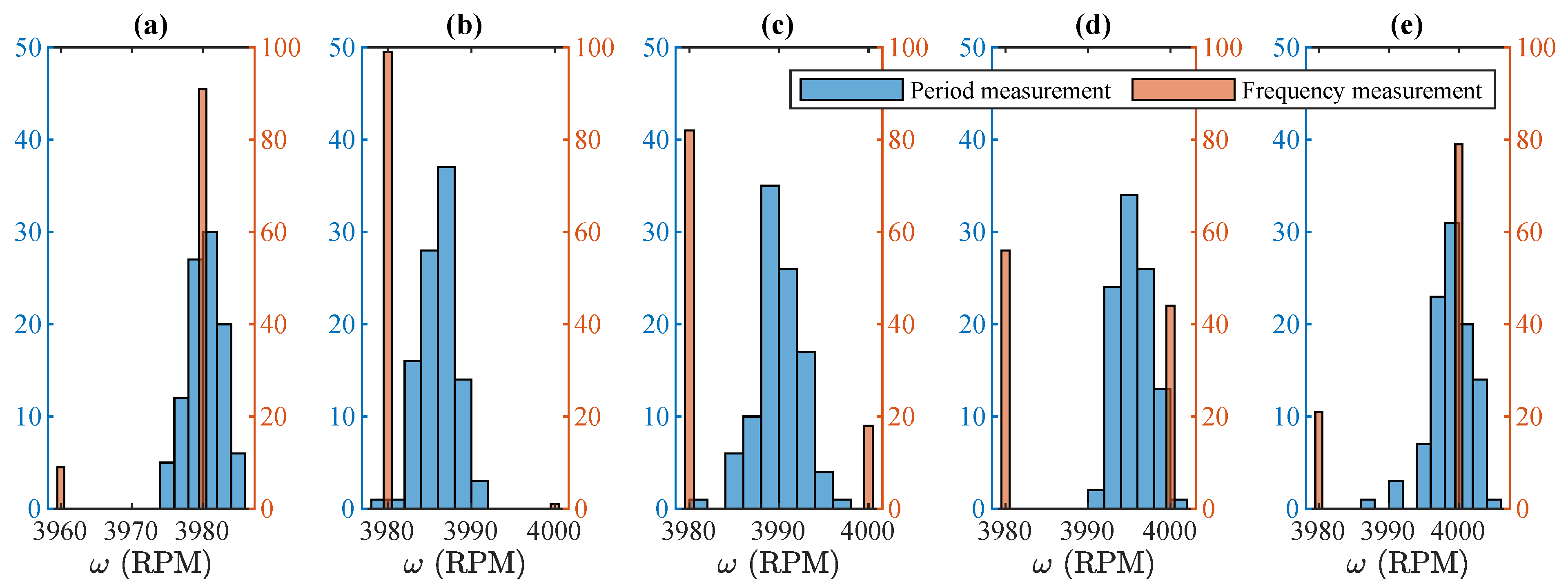
5.1. Steady-State Comparison

In this section, the analysis is made based on steady-state values with the test rig operating at constant angular speed values. The reference values considered were those provided by the frequency converter employed for driving the motor. For each test condition, 100 repetitions of the acquisitions were made, and both methods of computation were applied. The results around the lower end of the operating range are shown in Figure 6, while those around the higher end are shown in Figure 7.

From Figure 6, it can be observed that the period measurement method provides a mean centered at the reference, with a certain deviation around this value; on the other hand, the frequency method provides results limited to the method resolution, calculated at 20 $\mathrm{RPM}$ (2.09 rad s⁻¹) using (5) with $t_{\mathrm{w}}=0.05 \mathrm{s}$.

In Figure 6a, at around 1000 $\mathrm{RPM}$ (104.72 rad s⁻¹), despite the operating condition being an integer and multiple of the resolution provided by (5), the frequency method pointed to occurrences at 980 $\mathrm{RPM}$ (102.62 rad s⁻¹), resulting in a bias towards lower angular speeds. In Figure 6b, with the motor operating at 1005 $\mathrm{RPM}$ (105.24 rad s⁻¹), the frequency method shows only the occurrence of 1000 $\mathrm{RPM}$ (104.72 rad s⁻¹). In Figure 6c, with an operating angular speed of 1010 $\mathrm{RPM}$ (105.76 rad s⁻¹), which is in the middle point of two multiples of the resolution for this configuration (1000 $\mathrm{RPM}$ (104.72 rad s⁻¹) and 1020 $\mathrm{RPM}$ (106.81 rad s⁻¹)), the occurrences were not balanced, shifting towards a lower angular speed calculation. In Figure 6d,e this bias towards a lower angular speed calculation continues. The results in Figure 7 present similar results to those in Figure 6.

The mean values of the results shown in Figure 6 and Figure 7 are summarized in

Table 1. Difference between the means of the frequency method and period method when compared to a reference value.

${\mathit{\omega }}_{\mathbf{ref}}$ [RPM]	${\overline{\mathit{\omega }}}_{\mathbf{p}}$ [RPM]	$\mathit{E}{\%}_{\mathbf{p}}$ [%]	${\overline{\mathit{\omega }}}_{\mathbf{f}}$ [RPM]	$\mathit{E}{\%}_{\mathbf{f}}$ [%]
1000	999.7	−0.03	998.0	−0.20
1005	1004.3	−0.07	1000.0	−0.50
1010	1010.3	0.03	1001.6	−0.83
1015	1016.2	0.12	1012.6	−0.24
1020	1019.4	−0.06	1016.0	−0.39
3980	3980.4	0.01	3978.2	−0.05
3985	3986.0	0.02	3980.2	−0.12
3990	3990.0	0.01	3983.6	−0.16
3995	3995.5	0.01	3988.8	−0.16
4000	3998.9	−0.03	3995.8	−0.11

. In the table, ${\omega }_{\mathrm{ref}}$ is the reference angular speed, ${\omega }_{\mathrm{p}}$ is the angular speed calculated using the period method, $E{\%}_{\mathrm{p}}$ is the error between ${\omega }_{\mathrm{ref}}$ and ${\omega }_{\mathrm{p}}$, ${\omega }_{\mathrm{f}}$ is the angular speed calculated using the frequency method, and $E{\%}_{\mathrm{f}}$ is the error between ${\omega }_{\mathrm{ref}}$ and ${\omega }_{\mathrm{f}}$.

As shown in Table 1, the errors obtained by the period method were lower than those obtained using the frequency method for all operating conditions. The maximum error for the period method was 0.12%, which is 85% less than the maximum error for the frequency method ($-0.83\%$) in absolute terms. In addition, while ${\omega }_{\mathrm{p}}$ presented error values with positive and negative values, ${\omega }_{\mathrm{f}}$ presented only negative values, which is a bias towards lower angular speed estimates.

Finally, the acquired samples were used to calculate the resulting uncertainty based on Section 3. As an example, the step-by-step uncertainty assessment is shown for ${\omega }_{\mathrm{p}}$ when ${\omega }_{\mathrm{ref}}=$ 1000 $\mathrm{RPM}$ (104.72 rad s⁻¹). First, the mathematical relationship between the measured value ${\omega }_{\mathrm{p}}$ and the input quantities is presented in (10), and must be considered for the uncertainty assessment. Next, the input values are estimated. Because the value of $N_{\mathrm{p}}$ is fixed, the value of $t_{\mathrm{p}}$ is calculated for every pulse in the measurement window. After this, the uncertainty for every component is assessed based on the expressions deduced in Section 3.2. This is shown in

Table 2. Uncertainty components for ${\omega }_{\mathrm{p}}$ when ${\omega }_{\mathrm{ref}}=$ 1000 $\mathrm{RPM}$ (104.72 rad s⁻¹).

Uncertainty Component	DOF	Type	Probability Distribution	Standard Uncertainty [RPM]
$u_1\left({\omega }_{\mathrm{p}}\right)$	99	A	Normal	0.211
$u_2\left({\omega }_{\mathrm{p}}\right)$	∞	B	Rectangular	0.023
$u_3\left({\omega }_{\mathrm{p}}\right)$	∞	B	Rectangular	0.006
$u_4\left({\omega }_{\mathrm{p}}\right)$	32	B	Normal	0.375

, where the degrees of freedom (DOF), probability distribution, and standard uncertainty are assigned to each respective uncertainty component.

Equation (3) is used to combine the uncertainty components in Table 2, as they are assumed to be uncorrelated. The resulting expression is

$$\begin{array}{cc}\hfill u_c\left({\omega }_{\mathrm{p}}\right)& =\sqrt{{u_1\left({\omega }_{\mathrm{p}}\right)}^2+{u_2\left({\omega }_{\mathrm{p}}\right)}^2+{u_3\left({\omega }_{\mathrm{p}}\right)}^2+{u_4\left({\omega }_{\mathrm{p}}\right)}^2}\hfill \\ \hfill & =0.431.\hfill \end{array}$$

(29)

The measurement result is calculated using (10), resulting in ${\omega }_{\mathrm{p}}=$ $999.71$ $\mathrm{RPM}$ (104.69 rad s⁻¹). However, in order to properly represent this measurement result, the combined uncertainty assessed in (29) must be multiplied by a coverage factor k that depends on the effective degrees of freedom calculated using the Welch–Satterthwaite equation [16] and the desired level of confidence. For a 95% confidence, we have $k=2.0015$ and the measurement result is calculated as follows:

$$\begin{array}{cc}\hfill {\omega }_{\mathrm{p}}& ={\overline{\omega }}_{\mathrm{p}}\pm k·u_c\left({\omega }_{\mathrm{p}}\right)\hfill \\ \hfill & =(999.71\pm 0.86)\mathrm{RPM}.\hfill \end{array}$$

(30)

The same process described above was applied to the uncertainty assessments of the other operating conditions and the other method. The synthesis of the results is shown in

Table 3. Expanded uncertainty calculated for the frequency and period methods with the results acquired from the steady-state test. A total of 100 samples were considered for each uncertainty calculation.

${\mathit{\omega }}_{\mathbf{ref}}$ [RPM]	${\overline{\mathit{\omega }}}_{\mathbf{p}}$ [RPM]	$\mathit{U}\left({\mathit{\omega }}_{\mathbf{p}}\right)$ [RPM]	${\overline{\mathit{\omega }}}_{\mathbf{f}}$ [RPM]	$\mathit{U}\left({\mathit{\omega }}_{\mathbf{f}}\right)$ [RPM]
1000	999.71	0.86	998	23
1005	1004.29	0.85	1000	23
1010	1010.27	0.85	1001	23
1015	1016.24	0.85	1012	23
1020	1019.44	0.87	1016	23
3980	3980.43	0.93	3978	23
3985	3985.98	0.90	3980	23
3990	3990.01	0.94	3983	23
3995	3995.52	0.89	3988	23
4000	3998.89	0.99	3995	23

for a confidence of 95%, with $U\left({\omega }_{\mathrm{p}}\right)$ being the expanded uncertainty for the period method and $U\left({\omega }_{\mathrm{f}}\right)$ the expanded uncertainty of the frequency method. The uncertainties were assessed using the law of propagation of uncertainties in (3) for the uncertainty components in Section 3.

Based on the results shown in Table 3, the values of $U\left({\omega }_{\mathrm{p}}\right)$ are several times lower than those obtained for $U\left({\omega }_{\mathrm{f}}\right)$. The resulting resolution for $U\left({\omega }_{\mathrm{f}}\right)$ employing (5) is 20 $\mathrm{RPM}$ (2.09 rad s⁻¹), which is a direct result of the acquisition time window $t_{\mathrm{w}}=$ $0.05$ $\mathrm{s}$ and strongly impacts the final uncertainty results. As a consequence, the presented values of $U\left({\omega }_{\mathrm{f}}\right)$ are all assessed as 23 $\mathrm{RPM}$ (2.41 rad s⁻¹), due to the constant 20 $\mathrm{RPM}$ (2.09 rad s⁻¹) resolution, which is the main source of uncertainty and variability in the assessed values, being observed only in the decimal part. In addition, following directly from the discussion in Section 2, $U\left({\omega }_{\mathrm{p}}\right)$ is generally higher for higher operating angular speeds. The value of $U\left({\omega }_{\mathrm{p}}\right)$ for 3995 $\mathrm{RPM}$ (418.35 rad s⁻¹) was lower than expected for the angular speed as a result of a lower standard deviation observed in the experimental results.

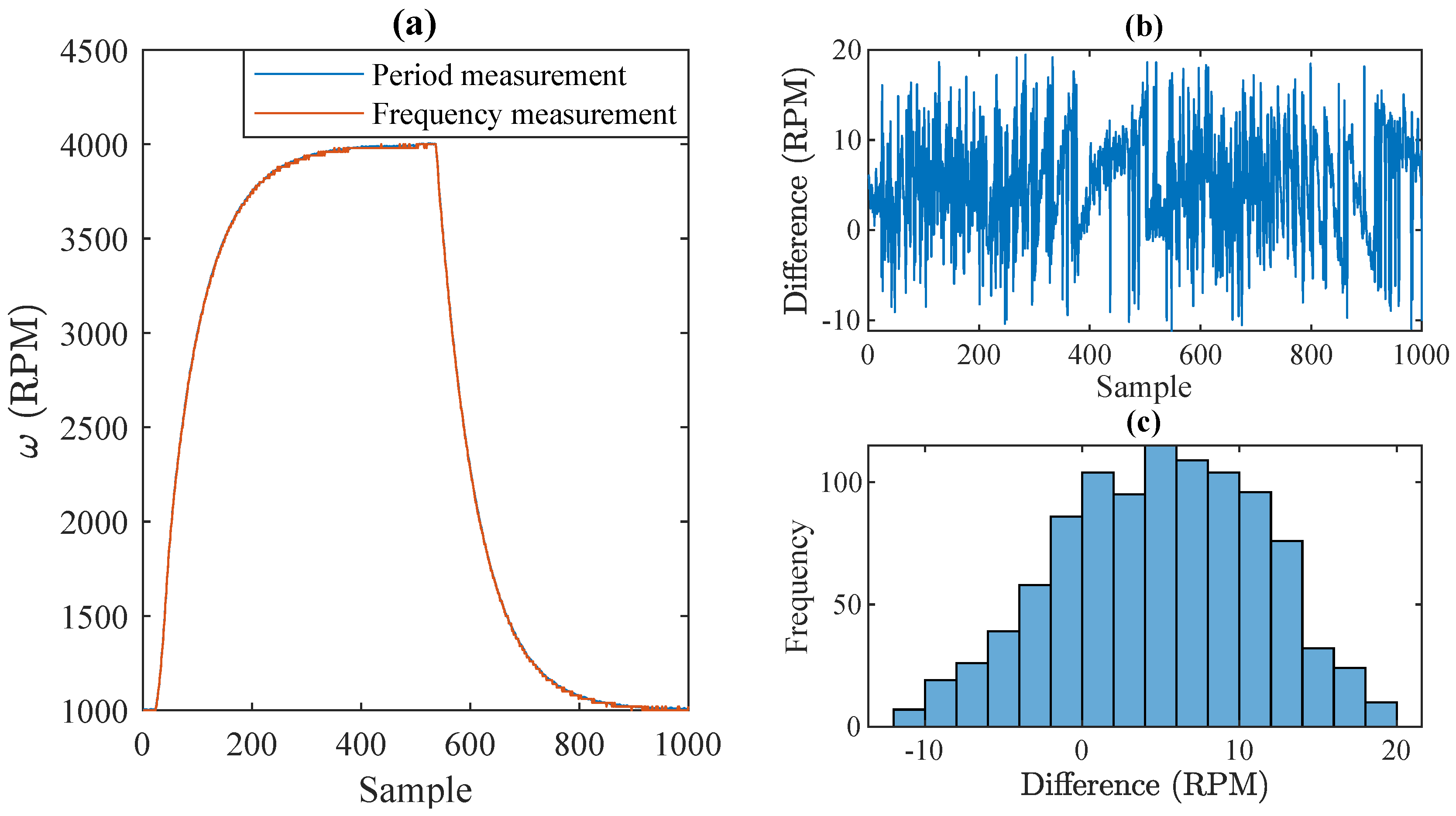
5.2. Dynamic Comparison

For the dynamic comparison between the frequency and period methods for angular speed calculation, the test rig was set to change the motor’s angular speed from 1000 $\mathrm{RPM}$ (104.72 rad s⁻¹) to 4000 $\mathrm{RPM}$ (418.88 rad s⁻¹) and then back to 1000 $\mathrm{RPM}$ (104.72 rad s⁻¹). The results are shown in Figure 8.

Considering the graphical analysis of the results in Figure 8a, when the angular speed reference is varied from 1000 $\mathrm{RPM}$ (104.72 rad s⁻¹) to 4000 $\mathrm{RPM}$ (418.88 rad s⁻¹), it seems that both curves overlap. However, if the point-by-point difference calculated between both methods is considered, as shown in Figure 8b, it is possible to note that the results of both methods are significantly different. This behavior is caused by the frequency method, which has results that oscillate around the value obtained by the period method. The histogram of Figure 8b is presented in Figure 8c, which shows that the frequency method varies between $-10$ $\mathrm{RPM}$ (−1.05 rad s⁻¹) and $20$ $\mathrm{RPM}$ (2.09 rad s⁻¹) around the value of the period method. This means that, because the value with the highest incidence is not zero, there is a inherent error when choosing the method. In this case, the difference between the methods is up to 20 $\mathrm{RPM}$ (2.09 rad s⁻¹), which is close to the expanded uncertainty of 23 $\mathrm{RPM}$ (2.41 rad s⁻¹) for the frequency method, as presented in Table 3. Although there are other components in the frequency method that define the overall uncertainty of the method, and although the uncertainty of the period method affects this difference as well, the frequency method’s resolution is the main cause in this case. This happens particularly because of the small acquisition time window required for proper dynamic characterization of the angular speed, which increases the method’s resolution.

6. Impacts on Efficiency Test Uncertainty

In this section, the impact of angular speed measurement uncertainty on electrical motor efficiency tests is assessed in the dynamometer detailed in Section 4 based on the results obtained in Section 5. In this section, the uncertainty components are combined using (3). It is worth noting that the results obtained in these analyses are strongly dependent on the instrumentation and parameters, namely, $f_{\mathrm{s}}$, $t_{\mathrm{w}}$, and $N_{\mathrm{p}}$. The uncertainty results obtained in this paper are related to the test rig detailed in Section 4; thus, the numerical values cannot be used for different setups. However, it is possible to determine the uncertainty components for any experimental setup by applying the equations deduced in Section 3.

To calculate the impact of the angular speed calculation method on the motor efficiency, the overall uncertainty of the components must be assessed as well. Starting with the efficiency calculation equation in (27), the efficiency uncertainty can be calculated as follows:

$$u{\left(\eta \right)}^2={\left(\frac{\partial \eta }{\partial \tau }u\left(\tau \right)\right)}^2+{\left(\frac{\partial \eta }{\partial \omega }u\left(\omega \right)\right)}^2+{\left(\frac{\partial \eta }{\partial P}u\left(P\right)\right)}^2,$$

(31)

where $u\left(\eta \right)$ represents the uncertainty of the motor efficiency, $\frac{\partial \eta }{\partial \tau }$ is the sensitivity coefficient related to the uncertainty of the torque $u\left(\tau \right)$, $\frac{\partial \eta }{\partial \omega }$ is the sensitivity coefficient related to the uncertainty of the angular speed $u\left(\omega \right)$, and $\frac{\partial \eta }{\partial P}$ is the sensitivity coefficient related to the uncertainty of the electrical power of the motor $u\left(P\right)$.

The test procedure in [17] was applied to this case considering two operating angular speed values of 1000 $\mathrm{RPM}$ (104.72 rad s⁻¹) and 4000 $\mathrm{RPM}$ (418.88 rad s⁻¹). A torque condition of 250 $\mathrm{m}$$\mathrm{N}$$\mathrm{m}$ was chosen as the midpoint of the available test range. A $4.5$ $\mathrm{h}$ waiting time was observed to allow for temperature settling in order to reduce the variability of the motor and bearing temperatures. After temperature settling, the acquisition ran for 300 $\mathrm{s}$. The room temperature was monitored and controlled within the range of $(23.0\pm 0.3) °\mathrm{C}$ by a central auxiliary system.

After data acquisition, the uncertainties were assessed for each quantity following its own set of components. The resulting uncertainties for the 1000 $\mathrm{RPM}$ (104.72 rad s⁻¹) tests are presented in

Table 4. Uncertainty components for the motor efficiency test considering an angular speed of 1000 $\mathrm{RPM}$ (104.72 rad s⁻¹) and calculation using the frequency method.

Quantity	Symbol	Mean	${\mathit{u}}_{\mathit{c}}$	U	Contribution (%)
Angular speed [RPM]	$\omega$	999.78	11.56	23	97.8
Torque [N.m]	$\tau$	250.01	0.16	0.33	0.3
Electrical power [W]	P	31.78	0.05	0.10	1.9
Efficiency [%]	$\eta$	82.36	0.96	1.90	100.0

for the frequency method and in

Table 5. Uncertainty components for the motor efficiency test considering an angular speed of 1000 $\mathrm{RPM}$ (104.72 rad s⁻¹) and calculation using the period method.

Quantity	Symbol	Mean	${\mathit{u}}_{\mathit{c}}$	U	Contribution (%)
Angular speed [RPM]	$\omega$	1000.31	0.38	0.75	12.3
Torque [N.m]	$\tau$	250.01	0.16	0.33	12.5
Electrical power [W]	P	31.78	0.05	0.10	75.2
Efficiency [%]	$\eta$	82.36	0.15	0.30	100.0

for the period method. For the 4000 $\mathrm{RPM}$ (418.88 rad s⁻¹) tests, the results are presented in

Table 6. Uncertainty components for the motor efficiency test considering an angular speed of 4000 $\mathrm{RPM}$ (418.88 rad s⁻¹) and calculation using the frequency method.

Quantity	Symbol	Mean	${\mathit{u}}_{\mathit{c}}$	U	Contribution (%)
Angular speed [RPM]	$\omega$	3999.99	11.56	23	89.8
Torque [N.m]	$\tau$	250.01	0.20	0.40	6.7
Electrical power [W]	P	119.74	0.07	0.14	3.5
Efficiency [%]	$\eta$	87.46	0.27	0.53	100.0

for the frequency method and in

Table 7. Uncertainty components for the motor efficiency test considering an angular speed of 4000 $\mathrm{RPM}$ (418.88 rad s⁻¹) and calculation using the period method.

Quantity	Symbol	Mean	${\mathit{u}}_{\mathit{c}}$	U	Contribution (%)
Angular speed [RPM]	$\omega$	3999.99	0.40	0.80	1.1
Torque [N.m]	$\tau$	250.01	0.20	0.40	65.6
Electrical power [W]	P	119.74	0.07	0.14	33.3
Efficiency [%]	$\eta$	87.46	0.09	0.17	100.0

for the period method.

The angular speed uncertainty in Table 4 was assessed using the components described in Section 3.1. In this case, it can be observed that the quantity with the greatest contribution to the efficiency uncertainty is the angular speed measured using the frequency method, which represents 97.8% of the overall contribution.

The angular speed uncertainty in Table 5 was obtained using the values in Section 3.2 for the period measurement method. The uncertainties for the remaining variables are the same as those listed in Table 4, as the measuring instruments and procedures were the same. It is notable that the contribution of the angular speed to the efficiency uncertainty dropped from 97.8% to 12.3%, without any changes to the test rig instrumentation. In addition, the expanded uncertainty for the motor efficiency dropped from $1.9\%$ to $0.3\%$.

For the 4000 $\mathrm{RPM}$ (418.88 rad s⁻¹) tests, on higher angular speeds (and consequently higher power consumption) there is an increase in the electrical power, which changes the balance of the uncertainty contributions. Considering the frequency method, the angular speed continues to present the higher contribution, as presented in Table 7, with a slight decrease from 97.8% to 89.8%. The contribution of the period method on lower angular speeds is 12.3%, with a decrease to 1.1% for the 4000 $\mathrm{RPM}$ (418.88 rad s⁻¹) test, as presented in Table 6. For the period method, lower angular speeds presented lower uncertainty, motivated by the dependence of the uncertainty upon the angular speed itself, as shown in (14), as expected based on the results depicted in Table 3. Due to the frequency method’s resolution, its uncertainty for all cases was 23 $\mathrm{RPM}$ (2.41 rad s⁻¹). When comparing the differences between the methods for the same condition, the period method was capable of reducing the overall contribution of the angular speed measurement from 89.8% to 1.1%. In terms of the motor efficiency uncertainty, this result represents a reduction from 0.53% to 0.17%.

7. Conclusions

This paper proposed an investigation of the impact of angular speed calculation methods on the uncertainty of electric motor efficiency tests. Our research begun by gathering the mathematical expressions to model the process of obtaining the angular speed based on the encoder measurements for both methods, then proceeded to analyze the acquisition configurations theoretically. Then, based on the mathematical expressions, the angular speed resolutions of both methods were obtained as functions of the operating conditions. Other sources of uncertainty were combined with the resolutions for assessing the measurement uncertainties of both methods following the procedures of the GUM. Finally, the theoretical results were experimentally validated using a dynamometer test rig.

The two angular speed calculation methods were tested simultaneously and the angular speed and motor efficiency uncertainties were calculated using the test data. Using the period method, it was possible to reduce the contribution of the angular speed uncertainty to the efficiency uncertainty by 87% at lower angular speeds and by 98% at higher angular speeds without any changes in the rig instrumentation. In addition, the differences between the calculated means and the reference values were lower when using the period method for all evaluated operating conditions. The maximum error for the period method was 85% lower than the maximum error for the frequency method. In addition, the frequency method presented a bias towards lower angular speed estimates.

The comparison of these two angular speed calculation methods across different angular speeds provides valuable insights into their impact on motor efficiency calculations. Our analysis reveals that the choice between frequency and period measurement methods can significantly influence the accuracy of efficiency assessments, particularly when evaluating small expected gains in motor performance. Moreover, the discussion above has underscored the relevance of addressing this gap in the literature, emphasizing the metrological implications of different angular speed calculation methods. Thus, the present study contributes to advancing the understanding of motor efficiency testing practices.

This research focused on studying the metrological aspects of the two most widely used methods for angular speed calculation using an encoder, and studied the impacts when propagating the angular speed uncertainties for the assessment of motor efficiency uncertainties. In future research, the proposed strategy can be used to obtain similar results for other angular speed calculation methods in the literature.

References

1. Dinolova, P.; Ruseva, V.; Dinolov, O. Energy Efficiency of Induction Motor Drives: State of the Art, Analysis and Recommendations. Energies 2023, 16, 7136. [Google Scholar] [CrossRef]
2. Ferreira, F.J.; de Almeida, A.T. Reducing Energy Costs in Electric-Motor-Driven Systems: Savings Through Output Power Reduction and Energy Regeneration. IEEE Ind. Appl. Mag. 2018, 24, 84–97. [Google Scholar] [CrossRef]
3. Caruso, M.; Tommaso, A.D.; Miceli, R.; Nevoloso, C.; Spataro, C. Uncertainty evaluation in the differential measurements of power losses in a power drive system. Measurement 2021, 183, 109795. [Google Scholar] [CrossRef]
4. IEC 60034-30-1:2014; Rotating Electrical Machines—Part 30-1: Efficiency Classes of Line Operated AC Motors (IE Code). International Eletrotechnical Comission: Geneva, Switzerland, 2006.
5. Aarniovuori, L.; Kolehmainen, J.; Kosonen, A.; Niemela, M.; Pyrhonen, J. Uncertainty in motor efficiency measurements. In Proceedings of the 17th International Conference on Electrical Machines and Systems, Hangzhou, China, 22–25 October 2014; IEEE: New York, NY, USA, 2014; pp. 323–329. [Google Scholar] [CrossRef]
6. Lu, S.M. A review of high-efficiency motors: Specification, policy, and technology. Renew. Sustain. Energy Rev. 2016, 59, 1–12. [Google Scholar] [CrossRef]
7. Kumar, R.; Sah, B.; Kumar, P. Stray Loss Formulation for Inverter-Driven Induction Motors for a Wide Range of Switching Frequency and Motor’s Loading. IEEE Trans. Ind. Electron. 2024, 71, 2385–2394. [Google Scholar] [CrossRef]
8. Song, Z.; Weidinger, P.; Kumme, R. Accurate Rotational Speed Measurement for Determining the Mechanical Power and Efficiency of Electrical Machines. In Proceedings of the 2021 24th International Conference on Electrical Machines and Systems (ICEMS), Gyeongju, Republic of Korea, 31 October–3 November 2021; pp. 1641–1645. [Google Scholar] [CrossRef]
9. Lorenz, R.; Van Patten, K. High-resolution velocity estimation for all-digital, AC servo drives. IEEE Trans. Ind. Appl. 1991, 27, 701–705. [Google Scholar] [CrossRef]
10. Briz, F.; Cancelas, J.; Diez, A. Speed measurement using rotary encoders for high performance AC drives. In Proceedings of the IECON’94—20th Annual Conference of IEEE Industrial Electronics, Bologna, Italy, 5–9 September 1994; Volume 1, pp. 538–542. [Google Scholar] [CrossRef]
11. Stojkovic, N.; Stare, Z.; Mijat, N. Dual-mode digital revolution counter. In Proceedings of the IMTC 2001, 18th IEEE Instrumentation and Measurement Technology Conference, Rediscovering Measurement in the Age of Informatics (Cat. No.01CH 37188), Budapest, Hungary, 21–23 May 2001; Volume 2, pp. 950–954. [Google Scholar] [CrossRef]
12. Petrella, R.; Tursini, M.; Peretti, L.; Zigliotto, M. Speed measurement algorithms for low-resolution incremental encoder equipped drives: A comparative analysis. In Proceedings of the 2007 International Aegean Conference on Electrical Machines and Power Electronics, Bodrum, Turkey, 10–12 September 2007; pp. 780–787. [Google Scholar] [CrossRef]
13. Ilmiawan, A.F.; Wijanarko, D.; Arofat, A.H.; Hindersyah, H.; Purwadi, A. An easy speed measurement for incremental rotary encoder using multi stage moving average method. In Proceedings of the 2014 International Conference on Electrical Engineering and Computer Science (ICEECS), Denpasar, Indonesia, 24–25 November 2014; pp. 363–368. [Google Scholar] [CrossRef]
14. Kazemirova, Y.; Podzorova, V.; Anuchin, A.; Lashkevich, M.; Aliamkin, D.; Vagapov, Y. Speed Estimation Applying Sinc-filter to a Period-based Method for Incremental Position Encoder. In Proceedings of the 2019 54th International Universities Power Engineering Conference (UPEC), Bucharest, Romania, 3–6 September 2019. [Google Scholar] [CrossRef]
15. Anuchin, A.; Podzorova, V.; Kazemirova, Y.; Chen, H.; Lashkevich, M.; Savkin, D.; Demidova, G. Speed Measurement for Incremental Position Encoder Using Period-Based Method with Sinc3 Filtering. IEEE Sens. J. 2023, 23, 5073–5083. [Google Scholar] [CrossRef]
16. JJCGM 100:2008; Evaluation of Measurement Data—Guide to the Expression of Uncertainty in Measurement. International Organization for Standardization: Geneva, Switzerland, 2008.
17. Machado, J.P.Z.; Flesch, R.C.C.; Schaefer, M.M.; de Santana, R.H. Bearing heating open-loop control system to reduce variability in BLDC motor tests. In Proceedings of the 2023 7th International Symposium on Instrumentation Systems, Circuits and Transducers (INSCIT), Rio de Janeiro, Brazil, 28 August–1 September 2023; pp. 107–112. [Google Scholar] [CrossRef]
18. Killedar, J. Dynamometer; Xlibris: Bloomington, IN, USA, 2012. [Google Scholar]
19. Blondel, A. Measurements of The Energy of Polyphase Currents. In Proceedings of the International Electrical Congress, Chicago, IL, USA, 21–25 August 1893; American Institute of Electrical Engineers: New York, NY, USA, 1894. [Google Scholar]
20. IEEE Std 115-2019 (Revision of IEEE Std 115-2009); IEEE Guide for Test Procedures for Synchronous Machines Including Acceptance and Performance Testing and Parameter Determination for Dynamic Analysis. IEEE: New York, NY, USA, 2020; pp. 1–246. [CrossRef]
21. Webster, J.G.; Eren, H. (Eds.) Measurement, Instrumentation, and Sensors Handbook, 2nd ed.; CRC Press: Boca Raton, FL, USA, 2014. [Google Scholar]
Figure 1. Period measurement method using a high-frequency counter with period T hf .
Metrology 04 00011 g001
Figure 2. Resolution for the frequency measurement method as a function of the number of encoder pulses per revolution and the acquisition time window.
Metrology 04 00011 g002
Figure 3. Resolution for the period measurement method as a function of the acquisition frequency and the operating angular speed. The number of pulses per revolution was fixed at N p = 60 .
Metrology 04 00011 g003
Figure 4. Resolution for the period measurement method considering the mean period among all pulses in a time window, as stated in (16), for two scenarios: (a) angular speed of 1000 RPM (104.72 rad s−1) and (b) angular speed of 4000 RPM (418.88 rad s−1).
Metrology 04 00011 g004
Figure 5. Test rig developed in [17] and employed for data acquisition in the experimental section of this paper.
Metrology 04 00011 g005
Figure 6. Dispersion of angular speed values around the lower operating region, showing a comparison of the two calculation methods. The reference values were (a) 1000 RPM (104.72 rad s−1); (b) 1005 RPM (105.24 rad s−1); (c) 1010 RPM (105.76 rad s−1); (d) 1015 RPM (106.29 rad s−1); and (e) 1020 RPM (106.81 rad s−1).
Metrology 04 00011 g006
Figure 7. Dispersion of angular speed values around the higher operating region, showing a comparison of the two calculation methods. The reference values were (a) 3980 RPM (416.78 rad s−1); (b) 3985 RPM (417.31 rad s−1); (c) 3990 RPM (417.83 rad s−1); (d) 3995 RPM (418.35 rad s−1); and (e) 4000 RPM (418.88 rad s−1).
Metrology 04 00011 g007
Figure 8. Measurements using the period and frequency methods: (a) time response when subjected to an angular speed reference change from 1000 RPM (104.72 rad s−1) to 4000 RPM (418.88 rad s−1) and back to 1000 RPM (104.72 rad s−1); (b) point-by-point difference between the responses in (a); (c) histogram representation of the point-by-point difference in (b).
Metrology 04 00011 g008