Article

Dynamic Multi-Relation Learning with Multi-Scale Hypergraph Transformer for Multi-Modal Traffic Forecasting

1
SHU-UTS SILC Business School, Shanghai University, Shanghai 201899, China
2
Smart City Research Institute, Shanghai University, Shanghai 201899, China
*
Author to whom correspondence should be addressed.
Future Transp. 2026, 6(1), 51; https://doi.org/10.3390/futuretransp6010051
Submission received: 20 January 2026 / Revised: 15 February 2026 / Accepted: 18 February 2026 / Published: 22 February 2026

Abstract

Accurate multi-modal traffic demand forecasting is key to optimizing intelligent transportation systems (ITSs). To overcome the shortcomings of existing methods in capturing dynamic high-order correlations between heterogeneous spatial units and decoupling intra- and inter-mode dependencies at multiple time scales, this paper proposes a Dynamic Multi-Relation Learning with Multi-Scale Hypergraph Transformer method (MST-Hype Trans). The model integrates three novel modules. Firstly, the Multi-Scale Temporal Hypergraph Convolutional Network (MSTHCN) achieves collaborative decoupling and captures periodic and cross-modal temporal interactions of transportation demand at multiple granularities, such as time, day, and week, by constructing a multi-scale temporal hypergraph. Secondly, the Dynamic Multi-Relationship Spatial Hypergraph Network (DMRSHN) innovatively integrates geographic proximity, passenger flow similarity, and transportation connectivity to construct structural hyperedges and combines KNN and K-means algorithms to generate dynamic hyperedges, thereby accurately modeling the high-order spatial correlations of dynamic evolution between heterogeneous nodes. Finally, the Conditional Meta Attention Gated Fusion Network (CMAGFN), as a lightweight meta network, introduces a gate control mechanism based on multi-head cross-attention. It can dynamically generate node features based on real-time traffic context and adaptively calibrate the fusion weights of multi-source information, achieving optimal prediction decisions for scene perception. Experiments on three real-world datasets (NYC-Taxi, -Bike, and -Subway) demonstrate that MST-Hyper Trans achieves an average reduction of 7.6% in RMSE and 9.2% in MAE across all modes compared to the strongest baseline, while maintaining interpretability of spatiotemporal interactions. This study not only provides good model interpretability but also offers a reliable solution for multi-modal traffic collaborative management.

1. Introduction

Traffic demand forecasting is a cornerstone of intelligent transportation systems (ITSs), playing a pivotal role in optimizing urban traffic management, scheduling resources, and providing real-time traveler information [1]. Accurate predictions empower authorities to mitigate congestion, reduce accidents, and enhance overall transportation efficiency. Early research primarily treated this task as a time series prediction problem, employing statistical methods like linear regression and ARIMA [2,3]. While effective for linear patterns, these approaches struggle to capture the complex, nonlinear, and spatiotemporal dependencies inherent in traffic data.
The advent of deep learning has revolutionized this field. Models such as Convolutional Neural Networks (CNNs) and Recurrent Neural Networks (RNNs), along with their variants (e.g., LSTMs, GRUs), demonstrated a superior capacity for modeling complex traffic modes [4]. Subsequently, graph neural networks (GNNs) [5,6] and spatiotemporal graph convolutional networks (STGCNs) [6] emerged as dominant paradigms, effectively capturing dependencies in non-Euclidean space defined by transportation networks. Despite these advancements, a significant limitation persisted: most studies focused on forecasting demand for a single transportation mode [7,8,9], overlooking the intricate interactions and spatiotemporal heterogeneity that characterize multi-modal urban systems. This narrow focus constrains the accuracy and generalizability of predictions in practical applications.
The availability of multi-source traffic data has recently spurred a shift towards collaborative forecasting frameworks. Leveraging data from multiple modes (e.g., taxi, bike, subway) enables not only improved accuracy for individual modes but also beneficial knowledge transfer from data-rich to data-sparse modes [10,11,12]. However, multi-modal forecasting faces two fundamental challenges rooted in data and model architecture.
(1)
Data heterogeneity and multi-scale spatiotemporal dynamics challenges.
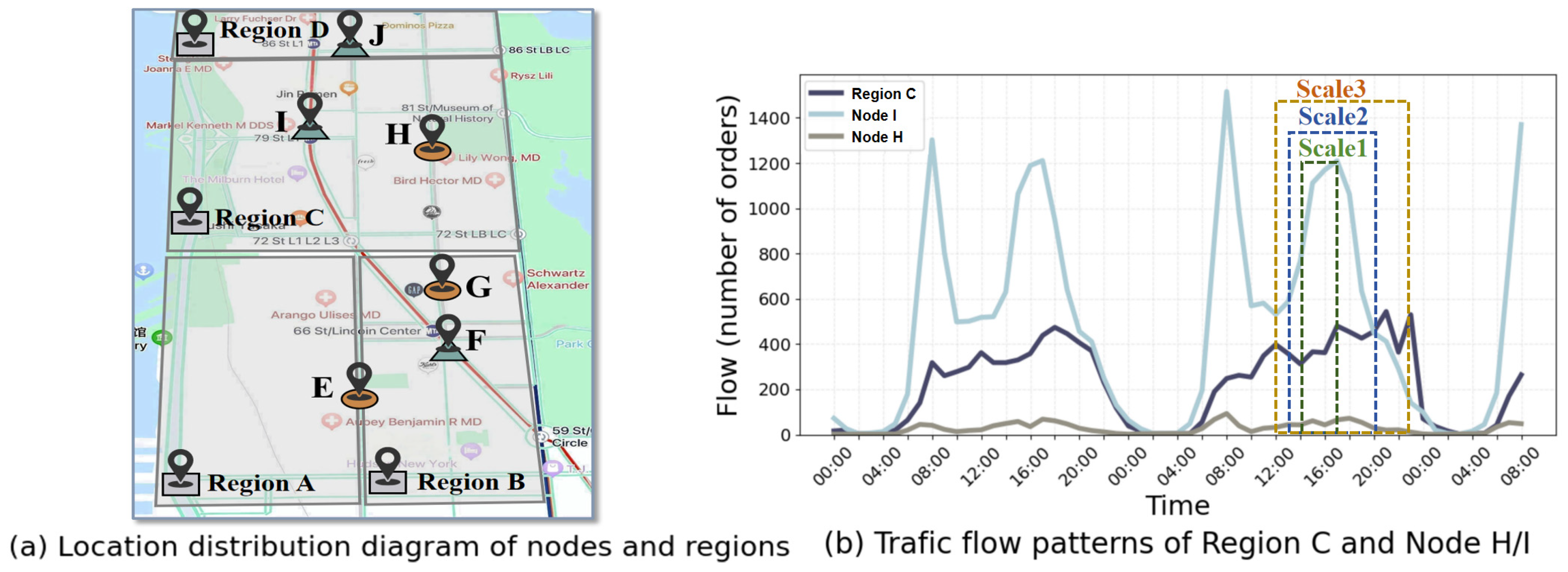
The core challenge of multi-modal traffic prediction lies in its inherent data heterogeneity and multi-scale spatiotemporal dynamics. This heterogeneity is manifested in two dimensions: spatial and temporal. Spatially, data from modes such as subway and bike-sharing are organized by fixed stations, whereas taxi data are aggregated based on grids or administrative regions. This mismatch in spatial units, as visualized in Figure 1a, hinders the effective alignment and integration of multi-source data. Temporally, even under the same scale, data magnitudes vary drastically across modes (e.g., subway daily flow reaches millions while bike-sharing demand is merely thousands), as shown in Figure 1b, making temporal correlation capture challenging. Crucially, spatiotemporal dynamics exhibit complex multi-scale characteristics where node relationships shift across scales (e.g., Scale 1 vs. Scale 3 in Figure 2). However, existing mainstream temporal models, such as TCN [13] or multi-resolution attention-based methods, typically rely on fixed window sizes or linear convolutions, making it difficult to adaptively capture periodic and cross-modal interactions in traffic data.
(2)
Limitations of dynamic and high-order spatial correlation modeling.
At the model architecture level, a key challenge is designing a framework that simultaneously captures intra-mode spatiotemporal features and dynamic inter-mode interactions. Existing graph-based methods (e.g., ST-MRGNN [12]) often depend on pre-defined or static graph structures, which cannot adapt to evolving spatial dependencies triggered by traffic conditions. Moreover, these methods are limited to pairwise relationships and cannot represent higher-order associations (e.g., multiple bike stations serving a subway hub). While hypergraph neural networks (HGNNs) [14] model high-order correlations, they typically use static hypergraph constructions [14,15,16,17,18], lacking real-time dynamism.
To address these gaps, we propose the Dynamic Multi-Relation Learning with Multi-Scale Hypergraph Transformer (MST-Hyper Trans). Unlike the above methods, MST-Hyper Trans introduces a multi-scale temporal hypergraph structure that can dynamically group data based on traffic cycles (such as time, day, and week), and merge hyperedges through Sørensen–Dice coefficients to adaptively decouple intra/inter-modal dependencies. To overcome the limitations of capturing spatially heterogeneous features, we designed a Dynamic Multi-Relationship Space Hypergraph Network (DMRSHN). Unlike traditional graph models, DMRSHN innovatively integrates geographic proximity, passenger flow similarity, and traffic connectivity to construct structural hyperedges and combines KNN and K-means algorithms to generate dynamic hyperedges, thereby accurately modeling high-order spatial correlations of dynamic evolution between heterogeneous nodes. Unlike traditional paradigms of spatiotemporal feature extraction and static fusion, our model introduces a novel collaborative perception dynamic generation context fusion paradigm. In summary, the main contributions are as follows:
  • Our framework leverages the Multi-scale Temporal Hypergraph Convolutional Network (MSTHCN) to extract multi-scale spatiotemporal features through collaborative temporal decoupling. Unlike existing multi-scale temporal methods (e.g., TCN [13]), which use uniform granularity and fixed convolutions, MSTHCN introduces a multi-scale temporal hypergraph structure that dynamically groups data based on traffic periodicity (e.g., hourly, daily, weekly scales) and merges hyperedges via the Sørensen–Dice coefficient. This enables adaptive capture of cross-modal temporal interactions and decouples intra-/inter-mode dependencies.
As summarized in Table 1, MSTHCN substantially improves modeling capability by integrating hypergraph convolution and attention mechanisms, overcoming the rigidity of TCN-like approaches.
2.
We design a dynamic feature generation and fusion mechanism via the Conditional Meta Attention Gated Fusion Network (CMAGFN). Traditional multi-modal prediction models often adopt static fusion strategies and cannot adaptively adjust according to real-time traffic scenarios. We introduced the Conditional Meta Attention Gated Fusion Network (CMAGFN) for this purpose. As a lightweight meta network, it dynamically generates node features based on real-time context (e.g., time, weather) and calibrates the fusion weights of multi-source information through a gate control mechanism based on multi-head cross-attention, achieving scene-aware adaptive optimal prediction decisions and significantly improving the adaptability and interpretability of the model.
3.
We have validated the superiority, effectiveness, and practical value of MST-Hyper Trans through extensive experiments on three real-world datasets. The experimental results indicate that our model significantly outperforms a series of baseline models. More importantly, in-depth ablation research and case analysis have shown that our model can provide new insights into cross-modal spatiotemporal interaction mechanisms, particularly demonstrating excellent predictive performance in sparse data scenarios, providing key guidance for the practical deployment of intelligent transportation systems.
The remainder of this paper is organized as follows: Section 2 reviews related work. Section 3 formalizes the problem. Section 4 details the MST-Hyper Trans architecture. Section 5 present the experimental setup and results/discussion, respectively. Section 6 concludes the paper.

2. Related Works

2.1. Traffic Demand Prediction Based on Convolutional Neural Networks

Convolutional Neural Networks (CNNs) are commonly employed in traffic demand forecasting because of their capacity to capture complex spatiotemporal patterns in traffic data. Ma et al. [19] introduced a hybrid architecture that combined CNNs and bidirectional long-term memory networks (BiLSTM) to predict passenger traffic in extensive subway networks. In 2021, Zhang et al. [20] proposed a CAS-CNN method featuring a channel attention mechanism and a split CNN to address data sparsity issues in short-term OD demand prediction for urban rail transit systems. Liang et al. [21] presented a Spatiotemporal Relational Network (STRN) for urban traffic prediction, utilizing CNN to extract local features from high-resolution urban traffic data, while incorporating global spatial dependencies and external factors through global relational modules and meta-learning modules, respectively. Qiao et al. [22] introduced a novel single-vehicle demand prediction model utilizing a Deep Convolutional Neural Network (DCNN) that incorporates diverse data sources such as weather and temporal information via a dynamic feature matrix. In the realm of multi-modal traffic demand prediction, Ye et al. [23] developed a sophisticated deep spatiotemporal neural network known as CoST-Net, which leverages convolutional layers and Long Short-Term Memory (LSTM) networks to capture spatiotemporal characteristics. Wang et al. [24] proposed the MultiST framework, employing Convolutional Neural Networks (CNNs) and gated recurrent units (GRUs) to extract spatiotemporal features across various traffic modes. Xu et al. [25] introduced the CMGAT framework by utilizing graph attention networks to model spatiotemporal dependencies among different traffic modes. Yang et al. [26] presented the Res-Transfer model, which integrates convolutional operations and attention mechanisms for feature extraction and inter-model correlation. However, CNN-based approaches require the transformation of the traffic network into a regular mesh network, thereby limiting their ability to capture spatial correlations within the traffic data.

2.2. Traffic Demand Prediction Based on Recurrent Neural Networks

Recurrent Neural Networks (RNNs) and their variants, such as Long Short-Term Memory (LSTM) and gated recurrent units (GRUs), have been pivotal in traffic demand forecasting. Lee and Ku [27] introduced a dual attention-based RNN model to predict bike-sharing demand. Wei et al. [28] integrated an attention mechanism with LSTM to capture key features in time series data and successfully predicted the passenger flow in the Hangzhou subway. Huang et al. [29] developed the MTLMetro model by utilizing LSTM within a multi-task learning framework to forecast subway demand. In the realm of multi-modal traffic demand forecasting, Zhang et al. [30] enhanced the short-term prediction accuracy of shared-bike usage by fusing historical shared-bike data with real-time public transport passenger data using LSTM. Huang et al. [10] employed a multi-modal dynamic graph convolution module and a gated loop unit to capture the dynamic effects of various traffic modes. Wang et al. [24] and Ye et al. [23] improved the multi-mode traffic demand prediction performance by extracting shared and unique spatiotemporal dependencies using technologies such as CNNs, GRUs, and deep spatiotemporal neural networks. In parallel to RNN approaches, researchers have also leveraged advanced architectures like Transformers for spatiotemporal modeling. For instance, Li et al. [31] proposed a Convolutional Transformer Network for vehicle trajectory prediction, which integrates convolutional layers for local spatial feature extraction with a Transformer encoder to capture long-range temporal dependencies. This work highlights the potential of hybrid architectures in complex urban traffic scenarios.
The emergence of deep learning technology has propelled temporal convolutional networks (TCNs) [13] to the forefront of research on traffic demand forecasting. Notably, Liu et al. [11] integrated a TCN and graph neural networks to model intricate spatiotemporal relationships among various traffic modes through multi-relationship graphs and introduced a novel approach to the collaborative prediction of multi-mode traffic demand. Similarly, Liang et al. [12] developed ST-MRGNN by leveraging TCN and a multi-graph neural network for the collaborative forecasting of multi-mode traffic demand. Building upon this, Liang et al. [32] enhanced multi-modal traffic demand forecasting by combining a TCN with a graph neural network. Furthermore, Zhang et al. [33] enhanced the performance of the joint prediction of multi-mode traffic spatiotemporal data by integrating a TCN, a graph sparse attention mechanism, and a bidirectional spatiotemporal convolutional network. Despite the notable achievements of Recurrent Neural Networks (RNNs) and their variants in traffic demand forecasting, the growing interest in TCN within this domain stems from its advantages of parallelism, flexibility, stability, and memory efficiency. However, TCN cannot adaptively group data based on the periodic flow in urban transportation systems for unified processing time scales, making it difficult to achieve the accurate prediction of peak hours for multiple transportation modes in cities.

2.3. Traffic Demand Prediction Based on Graph Convolutional Networks

Graph Neural Networks (GCNs) have transformed spatial feature extraction in traffic networks by modeling node relationships in non-Euclidean spaces. Several GCN variants have been introduced, such as STGCN [6], DCRNN [5], ASTGCN [34], and Graph WaveNet [35]. Moreover, Liu et al. [36] proposed a spatiotemporal attention graph convolutional network (ST-AGCN) for long-term public bicycle demand prediction. Gao et al. [37] developed a regularized spatiotemporal graph convolutional network (PMR-GCN) incorporating personalized enhanced graph convolutional networks and a multi-head self-attention mechanism to enhance accuracy and stability in subway passenger flow prediction. Wu et al. [38] proposed the TSHDNet, which employs a spatiotemporal heterogeneity decoupling gate to separate features from different traffic modes. Zhang et al. [39] combined Transformer networks, LSTM, and GCN to capture dependency relationships across multiple dimensions, enhancing subway passenger flow prediction performance. Additionally, Yang et al. [40] introduced DTG-MGCN, which leverages multi-graph convolution and dual time-domain gating branches to comprehensively consider nonlinear and spatial data correlations, thereby improving taxi demand prediction.
In studies focusing on collaborative forecasting of multi-mode traffic demand across heterogeneous spatial units, numerous researchers have employed graph neural networks to comprehend intricate spatial correlations among diverse traffic modes. Liu et al. [11] developed a self-learning heterogeneous traffic map alongside a space–time convolution module to autonomously discern spatial interdependencies among distinct traffic stations. They integrated multi-task learning networks to facilitate the collaborative prediction of multi-mode traffic demand. ST-MRGNN [12] introduced a multi-graph neural network to capture intricate spatiotemporal correlations among diverse traffic modes, enabling the collaborative prediction of heterogeneous traffic demand. In 2024, Li and Liu [41] devised a multi-modal traffic demand prediction model that leveraged federated learning. They introduced a fine-grained graph convolutional recurrent network (F-GCRN) to capture spatiotemporal correlations within traffic mode data. GSABT [33] established a flexible multi-mode traffic joint prediction framework by utilizing a graph sparse attention mechanism to extract spatial features, thereby enhancing the effectiveness of joint prediction.
However, a fundamental limitation persists across many of the graph-based methods mentioned above: they often rely on pre-defined or self-learning but essentially static graph structures, which struggle to capture the evolving spatial dependencies in dynamic traffic conditions. This issue is compounded when modeling associations between inherently heterogeneous spatial units (e.g., taxi regions vs. subway stations). Recent studies have thus begun to explore dynamic graph learning to address the first challenge. For example, Wei et al. [42] developed a dynamic graph convolutional network with an attention mechanism to adaptively learn the adjacency matrix.
Furthermore, the application of hypergraph neural networks has been extended to model higher-order correlations beyond pairwise relationships, offering a potential solution for complex heterogeneous interactions. The emergence of hypergraph learning techniques has, therefore, led to the adoption of hypergraph convolution methods for traffic demand prediction. Wang et al. [15] introduced a dynamic hypergraph convolutional network (DSTHGCN) to address the challenges posed by traditional graph neural networks in modeling intricate transportation networks. By constructing fundamental hypergraphs and advanced hyperedges, the DSTHGCN effectively captures the structural characteristics of subway networks and the evolving travel behaviors of passengers. Furthermore, Zhao et al. [16] presented a space–time hypergraph convolutional network (ALGHGCN) that incorporates a novel attention mechanism. By leveraging local and global hypergraph convolutions along with temporal attention mechanisms, the ALGHGCN adequately balances the local and global relationships in the data. In 2024, Ye et al. [17] developed a Dynamic Spatiotemporal Hypergraph Convolutional Network (DSTHGCN) that integrates collaborative convolution techniques from traffic flow graphs and hypergraphs to tackle the complexities associated with spatiotemporal modeling in traffic flow prediction. Additionally, Cao et al. [18] introduced the Spatial-Temporal Graph Hypergraph Convolutional Network (STGHCN), which combines hypergraph convolution with an attention mechanism to capture high-order spatial correlations across diverse traffic data types. Research on the application of hypergraph neural networks in multi-mode traffic demand collaborative forecasting is scarce. Wang et al. [43] introduced a multi-task hypergraph convolutional network (MT-HGCN) to enhance the prediction performance by leveraging multi-task learning and hypergraph convolutional networks to uncover internal correlations among various traffic mode data. Although hypergraph neural networks capture high-order correlations among multi-modal traffic nodes, there is still a need for further exploration into dynamically modeling heterogeneous traffic node graphs.
In summary, despite significant advances, the current literature on traffic demand forecasting exhibits three persistent gaps that this study aims to address. First, while graph-based methods and emerging dynamic hypergraph approaches (e.g., [15,42]) effectively model complex dependencies, they primarily focus on networks with homogeneous node types (e.g., only subway stations or only taxi zones), lacking a unified framework for collaborative forecasting across heterogeneous spatial units (e.g., regions, bike stations, subway stations). Second, existing methods often rely on static or semi-static graph structures, which are inadequate for capturing the high-order spatial correlations that evolve dynamically with traffic conditions. Third, and most critically, there is a lack of a dedicated mechanism that effectively decouples and models the intra- and inter-mode dependencies evolving over multiple time scales within a unified architecture for multi-modal systems.
Addressing this gap is crucial for developing practical intelligent transportation systems (ITSs), as urban mobility inherently involves interactions between multiple transportation modes operating in disparate spatial units. The inability to concurrently model dynamic, high-order correlations within and between these heterogeneous units limits the accuracy and generalizability of predictions in real-world scenarios.

3. Preliminaries

3.1. Notations and Definitions

3.1.1. Traffic Node

A traffic node refers to the spatial unit of a station within an urban transportation system, and can be categorized into two main types. The first type consists of stations with fixed locations, such as bus stops and subway stations, that can serve as nodes in a graph directly. The second type encompasses transportation modes without fixed stations, including those defined by order pick-up and drop-off points (such as bike-sharing services) and those defined by administrative regions (such as taxis). For bike-sharing services, this study employed a Density Peak Clustering (DPC) algorithm to cluster dispersed stations into virtual nodes. The regions themselves are treated as nodes for transportation modes defined by the administrative regions. In a multi-modal transportation system comprising r types of transportation modes, the i -th mode has n nodes, represented as the node set M i = { M i 1 ,   M i 2 ,   ,   M i n } , whereas the overall node set of the transportation system is denoted as M = { M 1 ,   M 2 ,   ,   M r } .

3.1.2. Traffic Demand and Node Features

In this study, the traffic demand of an urban traffic system is defined as the boarding demand x i ( t ) , which represents the number of vehicles traveling from node i to other areas during time step t . For each traffic node, a time series x i t : t + T is defined to indicate the boarding demand between times t and t + T . The node features refer to the transportation demand at node i . For traffic mode M i , in the demand study for time step t + 1 , the input node feature consists of the previous observations at time t, represented as X M i ( t ) = { x M i 1 ( t ) ,   x M i 2 ( t ) ,   ,   x M i n ( t ) } , where M i n denotes node n under traffic mode M i , and x M i n ( t ) is the traffic demand value at node n for time step t under traffic mode M i .

3.1.3. Multi-Modal Transportation System

Urban transportation system M consists of r ( w h e r e   r > 1 ) types of transportation modes, denoted as M i = { M 1 ,   M 2 ,   , M r } . Each transportation mode M i ( i = 1 ,   2 ,   ,   r ) has n m nodes, which serve as the basic units for the bidirectional flow of vehicles. At time step t , the demand characteristics of node i j ( j = 1 ,   2 ,   ,   n m ) under mode M i are represented by vector x M i n ( t ) . Thus, the characteristics of all the nodes under mode M i at time step t are represented by X M i ( t ) = { x M i 1 ( t ) ,   x M i 2 ( t ) ,   ,   x M i n ( t ) } . The demand representation for all nodes across all transportation modes in the urban transportation system at time step t is given as X t = { X M 1 ( t ) ,   X M 2 ( t ) ,   ,   X M r ( t ) } .

3.1.4. Heterogeneous Transportation Graph

A heterogeneous transportation graph is defined as G = ( V ,   E ) , where V represents the set of nodes and E represents the set of edges. The neighborhood relationship is defined as N ( v ) = { v V |   < u , v >   E } , where v ( v V ) denotes a node and e =   < u , v >   E represents an undirected edge between node v and node u .

3.2. Problem Definition

A traffic node refers to the spatial unit within an urban transportation system and can be categorized into two main types. The first type comprises stations with fixed locations, such as bus stops and subway stations. The second type encompasses transportation modes without fixed stations, including those defined by order pick-up and drop-off points (e.g., bike-sharing) and those defined by administrative regions (e.g., taxis).
The goal of the multi-modal traffic demand collaborative forecasting problem is to predict the future departure demands of various traffic modes for the next time interval. Specifically, we assumed that the multi-modal transportation system contained r traffic modes ( w h e r e   r > 1 ). The demand data for all the traffic modes are represented as X 1 : T = { X M i 1 : T | M i = M 1 ,   M 2 ,   ,   M i } . Given a historical time window of length L , the historical demand data for the multi-modal transportation system can be expressed as X T L : T = { X M i T L : T | M i = M 1 ,   M 2 ,   ,   M i } . We consider the intra-modal relationship graph G i n , inter-modal relationship graph G i n t e r , and external factor feature C E . Our objective is to learn a mapping function F ( · ) to jointly predict the demand for all traffic modes in the T + 1 time interval, as follows:
X T + 1 = F ( X T L : T , G i n , G i n t e r , C E )
where X T + 1 = { X M i T + 1 | M i = M 1 , M 2 , , M i } represents the demand for each traffic mode in the multi-modal transportation system during the next time interval, with X T + 1 R N . Here, L denotes the length of the historical time interval used for the prediction.
In addition, we have compiled all the variables and their meanings in this article into Table A1 in Appendix A.

4. Methodology

4.1. Network Architecture

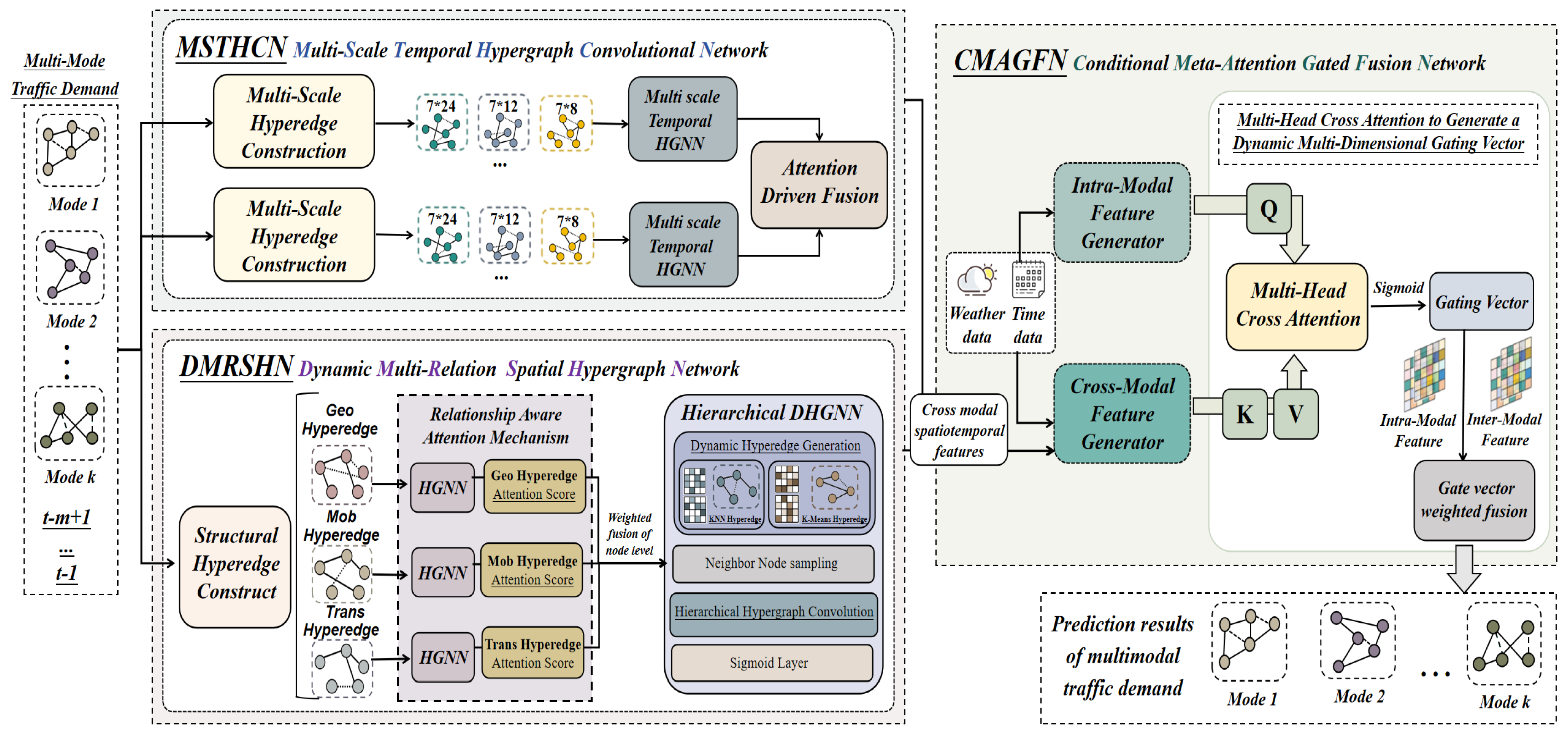
To bridge the gap in previous research, we propose the Multi-Scale Spatiotemporal Dynamic Hypergraph Transformer (MST-Hyper Trans). The novelty of our work lies in its integrated approach to dynamic multi-relation learning across spatial and temporal dimensions. Specifically, unlike prior works, (1) our model introduces a novel multi-scale temporal hypergraph (MSTHCN) to explicitly decouple and capture periodic and cross-modal temporal interactions at multiple granularities (e.g., hour, day, week). (2) We design a dynamic multi-relation spatial hypergraph network (DMRSHN) that integrates geographic proximity, passenger flow similarity, and transportation connectivity to construct both structural and dynamic hyperedges, enabling adaptive learning of high-order spatial correlations among heterogeneous nodes. (3) We introduce a Conditional Meta Attention Gated Fusion Network (CMAGFN) that dynamically generates and fuses features based on real-time context, moving beyond static fusion strategies. As shown in Figure 3, the model consists of three core modules, forming an end-to-end prediction process. This holistic framework represents a significant step towards accurate and interpretable collaborative forecasting for multi-modal urban transportation systems.
Firstly, the Multi-Scale Temporal Hyperedge Convolutional Network (MSTHCN) is responsible for handling the complexity of the temporal dimension. It effectively captures the periodic and trend patterns of transportation demand at different time granularities (such as hour, day, week) by constructing multi-scale temporal hypergraphs. The internal temporal attention mechanism can adaptively balance the contributions of different scale features, providing the model with powerful temporal representation capabilities. Secondly, the Dynamic Multi-Relationship Space Hypergraph Network (DMRSHN) focuses on modeling high-order dependencies between heterogeneous spatial units. This module integrates multiple semantic relationships, such as geographic proximity, passenger flow similarity, and transportation connectivity, to construct structural hyperedges, and generates dynamic hyperedges through KNN and K-means algorithms to capture spatial correlations that evolve with traffic conditions. The further introduction of a relationship-aware attention mechanism and a hierarchical hypergraph convolution structure achieve refined extraction and fusion of multi-relationship spatial features. Finally, the Conditional Meta Attention Gated Fusion Network (CMAGFN) serves as the decision core of the model, replacing the traditional static fusion approach. This lightweight meta network takes real-time context (such as time, weather, and real-time demand) as input and dynamically generates parameters. Through its core multi-head cross-attention gating mechanism, CMAGFN can adaptively calibrate the fusion weights of intra-mode features and cross-mode spatiotemporal features at the feature dimension level based on the current traffic scene, thereby achieving optimal prediction decisions.
MST-Hyper Trans has completed the complete prediction process from multi-scale temporal feature extraction, dynamic spatial relationship modeling, to context-aware fusion through the collaborative work of MSTHCN, DMRSHN, and CMAGFN modules, significantly improving the ability to accurately predict complex multi-modal transportation systems.

4.2. Multi-Scale Temporal Hypergraph Convolutional Network

To accurately capture the complex multi-scale temporal dependencies in multi-modal transportation demand, we propose the Multi-scale Time Series Hyperedge Convolutional Network (MSTHCN) module. This module significantly enhances the model’s ability to extract periodic, trending, and cross-modal temporal interaction features in transportation demand by combining hypergraph structure modeling with multi-scale temporal analysis. The MSTHCN method addresses the limitations of existing multi-scale temporal models (e.g., TCN) by leveraging multi-scale dynamic hyperedge merging to capture high-order temporal correlations and an attention mechanism for adaptive feature fusion, enabling real-time responsiveness to demand fluctuations in multi-modal traffic systems while mitigating overfitting. The overall structure of the MSTHCN core process includes three parts: multi-scale hyperedge construction, multi-scale temporal hypergraph convolution, and attention-driven fusion. Its structure is shown in Figure 4.
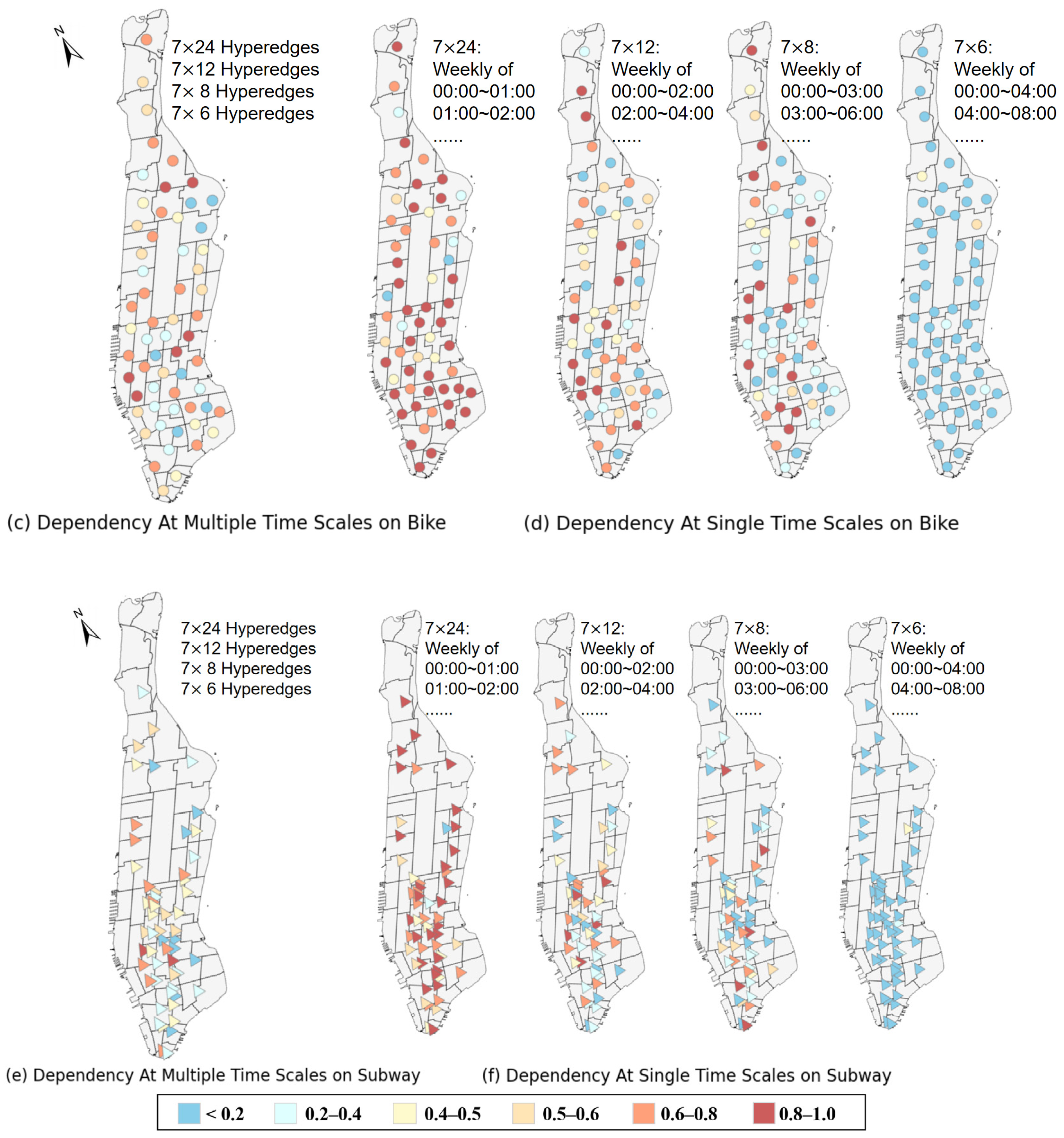
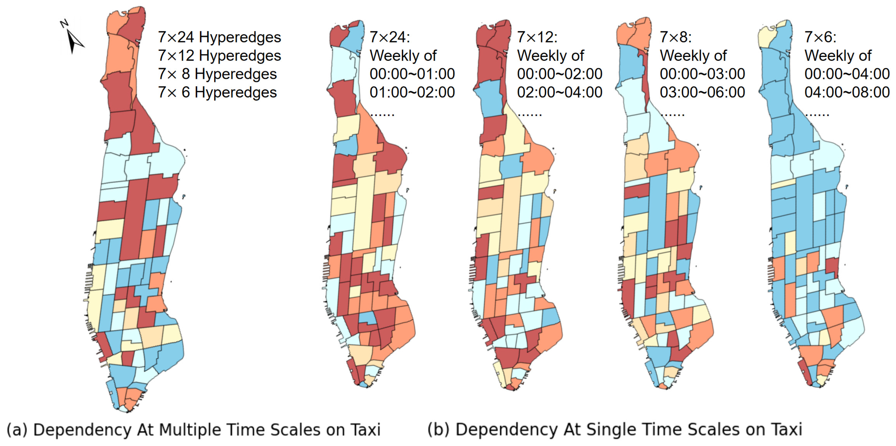
Inspired by multi-scale time series analysis methods, MSTHCN constructs hyperedges through grouping strategies (such as 1 h and 2 h granularity) and merges similar hyperedges (DSC > 0.8), which is more flexible than TCN’s fixed convolution kernel and can capture the periodicity of traffic demand (such as daily/weekly patterns). Specifically, for historical demand data { X t | t = 1 ,   2 ,   ,   T } , we grouped them by week and hour dimensions to generate four different time scale partitioning schemes: 1 h granularity (7 × 24 groups), 2 h granularity (7 × 12 groups), 3 h granularity (7 × 8 groups), and 4 h granularity (7 × 6 groups). Within each group, we retain the 40% data points with the highest and lowest demand values to form initial hyperedges in order to capture extreme traffic modes. Next, use the Sørensen–Dice coefficient (DSC) [44] to calculate the similarity between hyperedges:
D S C = 2 | H a H b | | H a | + | H b |
When the DSC value exceeds the threshold of 0.8, merge similar hyperedges to obtain a simplified hyperedge set { H ( q k ) | k { 1 ,   2 ,   3 ,   4 } ,   q k = 1 ,   , Q k } , where k represents the scale type, and q k is the hyperedge index. This design enables the model to adaptively capture multi-level time patterns from short-term fluctuations to long-term trends.
Multi-modal traffic data exhibits spatiotemporal heterogeneity. MSTHCN models high-order temporal correlations directly through hypergraph convolution, overcoming the limitation of traditional graph convolution that only deals with pairwise relationships. We use Spectral Hypergraph Convolutional Networks (HGNNs) [14] to separately process the temporal features within and between patterns. For the input signal X i n ( t ) within the pattern and the signal X i n t e r ( t ) between patterns, the hypergraph convolution operation is defined as:
X i n ( t + 1 ) = σ R e L U ( D ˇ v i n 1 / 2 H ~ i n W ~ i n D ~ e i n 1 H ~ i n T D ~ v i n 1 / 2 X i n ( t ) Θ i n )
X i n t e r ( t + 1 ) = σ R e L U ( D ˇ v i n t e r 1 / 2 H ~ i n t e r W ~ i n t e r D ~ e i n t e r 1 H ~ i n t e r T D ~ v i n t e r 1 / 2 X i n t e r ( t ) Θ i n t e r )
where H ~ i n and H ~ i n t e r are hypergraph correlation matrices with self-loops added, D ~ v and D ~ e are the degree matrices of nodes and hyperedges, respectively, and Θ is the learnable convolution kernel parameter. This process captures high-order temporal correlations between nodes through the hypergraph Laplacian operator, overcoming the limitation of ordinary graph convolution that can only model pairwise relationships.
To dynamically integrate temporal features within and between patterns, we introduce node-level attention weights to dynamically balance intra- and inter-mode features, while existing methods, such as multi-resolution attention, often rely on static weights. For node i , the attention weights of its intra- and inter-pattern features x i n i and x i n t e r i are calculated as follows:
a i n i = s o f t m a x ( W i n i X i n i + b i n i )
a i n t e r i = s o f t m a x ( W i n t e r i X i n t e r i + b i n t e r i )
where W i n i , W i n t e r i , b i n i , and b i n t e r i are learnable parameters. The temporal characteristic output of the final node i is:
Z M S T H C N i = a i n i X i n i + a i n t e r i X i n t e r i
This mechanism enables the model to adaptively adjust weights based on the current traffic context, highlighting dominant time patterns.

4.3. Dynamic Multi-Relation Spatial Hypergraph Network

Previous methods have had difficulty handling the complex heterogeneous spatial relationships between nodes in multi-modal transportation networks, as well as the characteristics of local and global relationships. The DMRSHN module captures complex high-order spatial dependencies between heterogeneous units (e.g., taxi regions and subway stations) by integrating domain knowledge via multi-relationship structured hyperedges, coupled with a relationship-aware attention mechanism and hierarchical hypergraph convolution for dynamic multi-scale spatial modeling. The DMRSHN module captures the complex high-order spatial relationships between multi-modal traffic nodes in the urban transportation system, as shown in Figure 5. The core of this network is to handle the dynamic evolution of multiple relationships (geographical proximity, passenger flow similarity, transportation connections), and to use hypergraph networks for high-order correlation modeling in the spatial domain, which can adaptively learn the spatial interactions between stations or regions under different transportation modes.
Firstly, the construction process of various structural hyperedges in the DMRSHN module’s multi-relationship structure hyperedge layer is introduced. The structural hyperedges mainly include geographical proximity hyperedges, passenger flow similarity hyperedges, and transportation connectivity hyperedges. The correlation matrix is mainly calculated between multi-mode transportation nodes, and then multiple hyperedges are obtained through threshold limitation. The calculation process of the relationship matrix is as follows:
(1)
Geographical Distance Embedding: For nodes i and j , which are spatial units categorized as regions, we define their distance matrix as A G r . For nodes i and j , which are spatial units categorized as sites, we define their distance matrix as A G s :
A G r = { 1 i f   i   a n d   j   a r e   a d j a c e n t exp ( ( d i j σ d ) 2 ) i f   i   a n d   j   a r e   n o t   a d j a c e n t   a n d   d i j k d r 0 i f   i   a n d   j   a r e   n o t   a d j a c e n t   a n d   d i j > k d r
A G s = { exp ( ( d i j σ d ) 2 ) i f   d i j k d s 0 i f   d i j > k d s
Here, A G r represents the weight of the geographical proximity between regions i and j , d i j is the distance between the geometric centers of regions i and j , k d r is the distance threshold, and σ d is the standard deviation of the distance. Similarly, A G s denotes the weight of geographical proximity between sites i and j , where d i j is the distance between sites i and j , and k d s is the distance threshold.
For node i with spatial units defined as regions and node j with spatial units defined as points, we define the distance matrix as A G r s . Specifically, when node j is located within region i , we set A G r = 1. When node j is not within the region i , we define d i j as the shortest distance from node j to region i , and the weight is calculated using the method described in Equation (9).
(2)
Passenger Flow Similarity Embedding: The historical demand sequences of all nodes are normalized, and the similarity between nodes is computed using correlation coefficients. The passenger flow similarity embedding matrix A P is defined as follows:
A p = { C o r r ( p i , p j ) σ p , i σ p , j C o r r ( p i , p j ) σ p , i σ p , j k p 0 C o r r ( p i , p j ) σ p , i σ p , j < k p
In this context, A p represents the weight of similarity in passenger flow variation patterns between nodes i and j . The normalized historical demand sequences for nodes i and j are denoted as p i and p j , respectively. The term C o r r ( ) refers to the correlation coefficient used to calculate the relationship between two time series. Threshold k p is determined based on the sparsity of A p , whereas σ p , i and σ p , j represent the standard deviations of p i and p j , respectively.
(3)
Traffic Transfer Embedding: When embedding heterogeneous graphs, incorporating domain-specific knowledge can enhance the learning effectiveness of heterogeneous node features [45]. To achieve this, we constructed the traffic transfer embedding matrix A C o n to capture the transfer relationships of multi-modal passenger traffic flow. For any two nodes i and j , we define their traffic transfer embedding matrix A C o n :
A C o n i , j = { t = 1 T C i j t = 1 T j = 1 N C i j t = 1 T C i j t = 1 T j = 1 N C i j k C   a n d   d i j D 0 t = 1 T C i j t = 1 T j = 1 N C i j < k C   o r   d i j > D
In this context, A C o n i , j represents the traffic connection relevance weight from node i to node j , and C i j denotes the number of passengers boarding at node j within 15 min of alighting from node i . Variable d i j indicates the distance between two nodes, D is the distance threshold, and k C serves as the threshold for controlling sparsity. Notably, A C o n i , j is typically not equal to A C o n j , i , reflecting the directional nature of the transfer relationship.
For the three types of relationship matrices, we establish thresholds δ G , δ P , and δ C , and generate three types of hyperedges for each node based on these thresholds. Then, the similarity between any two super edges in the three super edge sets is calculated by using the Sørensen–Dice coefficient. Combine the super edges with a Sørensen–Dice coefficient less than 0.8 to obtain three relational super edge sets, which are defined as H G = { h e 1 , h e 2 , , h e G } ,   H P = { h e 1 , h e 2 , , h e P } ,   H C o n = { h e 1 , h e 2 , , h e C o n } .
In the relationship-aware attention mechanism layer, we first perform the hypergraph convolution operation based on the initial hyperedge set corresponding to each relationship type (i.e., the geography, passenger flow, and connection hyperedge set before the merger), and obtain the preliminary feature representation of node i under the three relationship types:
Z i G = σ R e L U ( D ˇ v 1 / 2 H ~ G W ~ G D ~ e 1 H ~ G T D ~ v 1 / 2 X M Θ G )
Z i P = σ R e L U ( D ˇ v 1 / 2 H ~ P W ~ P D ~ e 1 H ~ P T D ~ v 1 / 2 X M Θ P )
Z i C = σ R e L U ( D ˇ v 1 / 2 H ~ C o n W ~ C o n D ~ e 1 H ~ C o n T D ~ v 1 / 2 X M Θ C o n )
where H G ,   H P ,   and   H C o n are hyperedge incidence matrices of three relationship types respectively, X M is the input characteristics of nodes, and θ is a learnable parameter matrix.
Note that Equations (15)–(17) define the relationship-aware attention mechanism, which is proposed in our work to dynamically fuse spatial features from different relational hyperedges (geographic, passenger flow similarity, and connectivity). The attention score s i k for node i and relation type K is computed by a single-layer MLP (Equation (15)) based on the concatenation of the current node feature and the relation-specific feature. The final attention weights a i k are obtained by normalizing these scores using the Softmax function (Equation (16)), which are then used to compute the weighted sum of the relation-specific features to yield the final spatial representation Z i s p a t i a l (Equation (17)). This design allows the model to adaptively prioritize the most relevant spatial relationship for each node under specific traffic contexts.
For node i and relationship type K   { G ,   P , C } , we splice its current node feature X i M with the feature representation Z i k under relationship type k, and calculate the attention score s i k through a single-layer MLP and Leaky-Relu activation function:
s i k = L e a k y R e L U ( w T [ x i Z i k ] )
where [ · · ] represents vector splicing operation and w is a learnable attention vector.
Then use the Softmax function to normalize the attention scores of the three relationship types to obtain the normalized attention weight a i k :
a i k = exp ( s i k ) k { G ,   P ,   C } exp ( s i k )
Finally, the spatial feature Z i s p a t i a l of node i after the fusion of the relationship-aware attention mechanism is the weighted sum of three relationship features:
Z i s p a t i a l = a i G Z i G + a i P Z i P + a i C Z i C
Through the relationship-awareness mechanism, the model can adaptively allocate different importance weights for geographical proximity, passenger flow similarity, and traffic connectivity according to the specific traffic context, so as to achieve a more refined modeling of heterogeneous spatial dependencies.
In order to overcome the shortcomings of traditional multi-scale convolution kernel parallel processing in feature hierarchy, we propose a hierarchical hypergraph convolution structure. The structure of hierarchical hypergraph convolution is shown in Figure 6. Through the serial stacking and residual connection of three layers of convolution, our hierarchical design achieves the gradual expansion of information perception range layer by layer, effectively simulating the progressive process of human cognition from local details to global patterns. Compared to simple parallel multi-scale convolution, this method can generate more hierarchical and rich feature representations, thus better serving multi-modal traffic prediction tasks. Equations (18)–(21) describe the hierarchical hypergraph convolution process, a novel design in our work for multi-scale spatial feature extraction. Inspired by the success of hierarchical convolution in CNNs for capturing features at different receptive fields [46], we apply hypergraph convolutional kernels of increasing effective sizes (e.g., 1 × 1, 3 × 3, 5 × 5) to the KNN and K-means hypergraphs. The outputs from different levels are fused through residual connections (Equations (19) and (20)), enabling the model to progressively capture local-to-global spatial dependencies. The final inter-modal spatial feature Z i n t e r _ S T is obtained by concatenating and linearly transforming the features from different hypergraph types (Equation (21)).
The dynamic super edge generation layer samples KNN and K-means neighbor nodes based on the node structure characteristics generated by the relationship-awareness layer, and generates KNN super edge and K-means super edge, that is, the node set represented by H N N e = { u 1 , u 2 , , u N N } , H K M e a n s e = { u 1 , u 2 , , u K M e a n s } and the node set represented by H N N u = { h 1 , h 2 , , h N N } , H K M e a n s u = { h 1 , h 2 , , h K M e a n s } .
After completing the construction of KNN hyperedges and K-means hyperedges in the dynamic hyperedge construction layer, this paper constructs a hierarchical hypergraph convolution layer. Multiple layers of different sized convolution kernels are applied to the KNN hypergraph and K-means hypergraph, respectively. Then, the feature representations obtained from different levels of convolution are fused. The calculation process for hierarchical convolution of KNN hyperedges and K-means hyperedges is as follows:
Z N N ( 1 ) = σ R e L U ( D ˇ v 1 / 2 H ~ N N W ~ N N D ~ e , N N 1 H ~ N N T D ~ v 1 / 2 Z s p a t i a l Θ N N 1 × 1 )
Z N N ( 2 ) = σ R e L U ( D ˇ v 1 / 2 H ~ N N W ~ N N D ~ e , N N 1 H ~ N N T D ~ v 1 / 2 Z s p a t i a l Θ N N 3 × 3 ) + Z N N ( 1 )
Z N N = σ R e L U ( D ˇ v 1 / 2 H ~ N N W ~ N N D ~ e , N N 1 H ~ N N T D ~ v 1 / 2 Z s p a t i a l Θ N N 5 × 5 ) + Z N N ( 2 )
Z i n t e r _ S T = W c [ Z N N Z K M e a n s Z M S T H C N ] + b c
where [ · · ] is the splicing operation and W c is the learnable weight matrix. Z i n t e r _ S T is the spatial feature representation finally obtained by the DMRSHN module. Z N N and Z K M e a n s are the feature representations obtained by the hierarchical convolution of the KNN super edge and K-means hyperedge, respectively. The algorithmic principles of the DMRSHN module are presented in Algorithm A1 in Appendix B.

4.4. Conditional Meta Attention Gated Fusion Network

The CMAGFN module overcomes the static limitations of traditional fusion strategies by incorporating a gated fusion mechanism based on multi-head cross-attention, which dynamically calibrates feature weights for context-aware decision-making. As a lightweight meta network, CMAGFN can dynamically generate fusion weights based on real-time context, rather than relying on static parameters. It can dynamically calculate a fine-grained multidimensional gating vector (rather than a single scalar) based on real-time traffic context, thereby adapting the contribution weights of intra-mode features and cross-mode features at the feature dimension level, and achieving more accurate and interpretable feature fusion. Equations (22)–(30) formulate the core of the Conditional Meta Attention Gated Fusion Network (CMAGFN), a key contribution of this paper. The intra- and inter-modal features are first projected by lightweight MLPs (Equations (22) and (23)). The multi-head cross-attention mechanism (Equations (24)–(27)), drawing inspiration from the transformer architecture [47], is employed to compute the context-aware gating vector g i m h (Equation (28)), where the query is the intra-modal feature, and the key/value are derived from the inter-modal features. This allows the model to dynamically assess the relevance of cross-modal information for each feature dimension. The final fused feature x i f i n a l is a weighted sum of the intra- and inter-modal features under the control of this gating vector (Equation (29)). The entire process is designed to replace static fusion strategies, enabling fine-grained, adaptive feature integration.
The overall architecture is illustrated in Figure 7, which enables the dynamic optimization of the entire process, from information filtering to feature fusion, through an attention mechanism. The input of the CMAGFN layer is a context vector that comprehensively describes the current traffic status, ensuring that the generated dynamic weights can respond to real-time conditions. It mainly includes core environment context, intra-pattern requirement context, and cross-pattern context, where the core environment context includes timestamps (such as hour, day of the week) and weather conditions (such as sunny, rainy) encoded by embedding layer vectors C t and C w , respectively. The intra-pattern requirement context C i n t r a refers to the recent historical demand sequence of nodes in the target transportation mode (e.g., taxi), which is extracted using a lightweight temporal convolutional layer. The cross-modal context includes the pure historical demand sequence C i n t e r _ h i s t of the relevant patterns, as well as the fused spatiotemporal features Z i n t e r _ S T from the MSTHCN and DMRSHN modules. For each node, CMAGFN includes two parallel lightweight MLP paths that generate feature representations optimized for intra-pattern and cross-pattern information, respectively. The intra-model feature generator focuses on learning from the contextual requirements and core environment within the pattern, capturing the historical patterns of the pattern itself.
Z i i n t r a = M L P i n t r a ( [ C t C w C i n t r a ] )
The cross-modal feature generator focuses on learning from all cross-modal contexts and core environmental contexts, extracting synergistic effect information provided by other traffic modes.
Z i i n t e r = M L P i n t e r ( [ C t C w C i n t e r _ h i s t Z i n t e r _ S T ] )
where Z i i n t r a , Z i i n t e r R d , d is the feature dimension.
The core of the CMAGFN module is to use multi-head cross-attention to generate a dynamic multi-dimensional gating vector. The query Q is derived from the output Z i n t r a of the intra-modal feature generator, which is obtained through linear transformation and represents the current node’s own state in the target pattern. The key K and value V are derived from the output Z i n t e r of the cross-modal feature generator and obtained through linear transformation, representing the contextual information provided by other modals:
Q = Z i i n t r a × W Q , K = Z i i n t e r × W K , V = Z i i n t e r × W V
where W Q , W K , and W V are learnable parameter matrices.
Subsequently, calculate the attention score and apply Softmax to obtain the weights:
A t t e n t i o n ( Q , K , V ) = S o f t m a x ( Q K T d k ) V
where d k is the dimension of the key vector K, and the scaling factor 1 d k is used to prevent gradient vanishing due to excessive dot product results.
After computing the query (Q), key (K), and value (V), the CMAGFN module performs multi-head attention mechanism calculations by using multiple sets of different WQ, WK, and WV matrices to perform h parallel attention calculations as described above. Each head focuses on different aspects of the input information, and finally concatenates the outputs of each head:
M u l t i H e a d ( Q , K , V ) = C o n c a t ( h e a d 1 , , h e a d h ) W O
h e a d i = A t t e n t i o n ( Q W i Q , K W i K , V W i V )
where W O is the output projection matrix.
The multi-head attention mechanism enables the model to evaluate the relationships between features from different subspaces, thereby gaining a more comprehensive understanding of cross-modal interactions. The CMAGFN module passes the output of multi-head attention through a linear layer and Sigmoid activation function to generate a multidimensional gating vector g i m h :
g i m h = σ ( W g · M u l t i H e a d ( Q , K , V ) + b g )
The distribution of gate control vector g i m h can directly reflect the degree of dependence of the model on intra- and cross-modal information in different contexts, providing insights for decision-making. Ultimately, the fusion feature x i f i n a l of node i is the weighted sum of intra-pattern features and cross-pattern features under this gating vector:
x i f i n a l = g i m h Z i i n t r a + ( 1 g i m h ) Z i i n t e r
where ⊙ represents the Hadamard product. This design allows the model to adopt different fusion strategies in different feature dimensions, achieving extremely refined fusion.


4.5. Multi-Task Learning Strategies

Based on the method for modeling task weights with homoscedastic uncertainty proposed by Kendall et al. [48], we set the loss weights for each task to be adaptively learned within the loss function (Equation (30)) by utilizing a multi-task learning strategy. The training objective of our model is to minimize the error between the predicted demand x ^ and the actual demand x across all patterns and nodes. The loss function is defined as the mean squared error (MSE) between the predicted and actual values and is mathematically expressed as follows:
L ( θ ) = k   = 1 r ( 1 σ k 2 i = 1 N k x ^ k , i t + 1 x k , i t + 1 ) + γ θ 2 2
In this context, x ^ k , i t + 1 and x k , i t + 1 represent the predicted and actual demand values for node i of pattern k at time step t + 1 , respectively. The noise variance for task k is given by σ k 2 = e x p ( l o g _ v a r s [ k ] ) , and is a learnable parameter. Term 1 σ k 2 serves as the adaptive weight, whereas l o g σ k acts as a regularization term. Here, N k denotes the number of nodes in the k -th traffic mode, and γ is the weight of the L2 regularization term. The training process for the proposed model is presented in Algorithm 1.
Algorithm 1: The training process of MST-Hyper Trans
Input: historical demand data X T L : T = { X M i T L : T ,   M i } , intra-modal multi-time scale hypergraph G T _ i n t r a = ( V i n t r a ,   E i n t r a ,   A i n t r a ) inter-modal multi-time scale hypergraph G T _ i n t e r = ( V i n t e r ,   E i n t e r ,   A i n t e r ) , Weather data C w , time data C t , number of MDHGNN layers L , number of training epochs E
Output: prediction demand value X T + 1 = { X M i T + 1 ,   M i }
Initialize the parameters of MST-Hyper Trans;
Initialize its input dim, hidden dim and output dim;
Generate training loader;//Training loader format is [input length, number of vertex, input]
For  e in { 1 ,   2 , E }  do
  Initialize H i n as X T L : T for all modes, initialization of H i n , m as X m T L : T for each mode m { 1,2 , k } ;
  For  m { 1,2 , k }  do
    Compute Z M S T H C N from a MSTHCN layer given H i n , H i n , m , G T _ i n t r a , G T _ i n t e r ;
    Compute Z i n t e r _ S T from DMRSHN layer given Z M S T H C N ;
    Compute H H A from CMAGFN given Z i n t e r _ S T , C t , C w ;
    Generate predictions X ^ m t + 1 from H H A using a mode-specific output layer;
  End
  Calculate the loss function Equation (30) from prediction results { X ^ m t + 1 ,   m { 1 ,   2 ,   k } } ;
  Update the parameters through error back propagation;
End

5. Experiments

5.1. Data Description

To validate the effectiveness of the proposed model, we conducted experiments on three real-world traffic datasets—NYC-Taxi, NYC-Bike, and NYC-Subway—collected from Manhattan, New York City, covering the period from 1 April to 30 June 2023.
The spatial units for each mode were defined differently. The taxi data were aggregated into irregular regions based on the Neighborhood Tabulation Areas (NTAs) defined by the New York City Department of City Planning. The bike-sharing and subway data were organized into virtual stations and physical stations, respectively. Each spatial unit across all datasets was assigned a unique numerical identifier. Key data fields include geographic coordinates (latitude and longitude) for trip start and end points, precise timestamps, and trip distances (for taxi) or passenger counts (for subway). Additionally, we integrated hourly weather data from the Central Park station, incorporating features such as temperature, humidity, precipitation, and snowfall after data cleaning.
A quantitative summary of the key statistics for these datasets is provided in Table 2 offering a concise overview of their scale and structure.
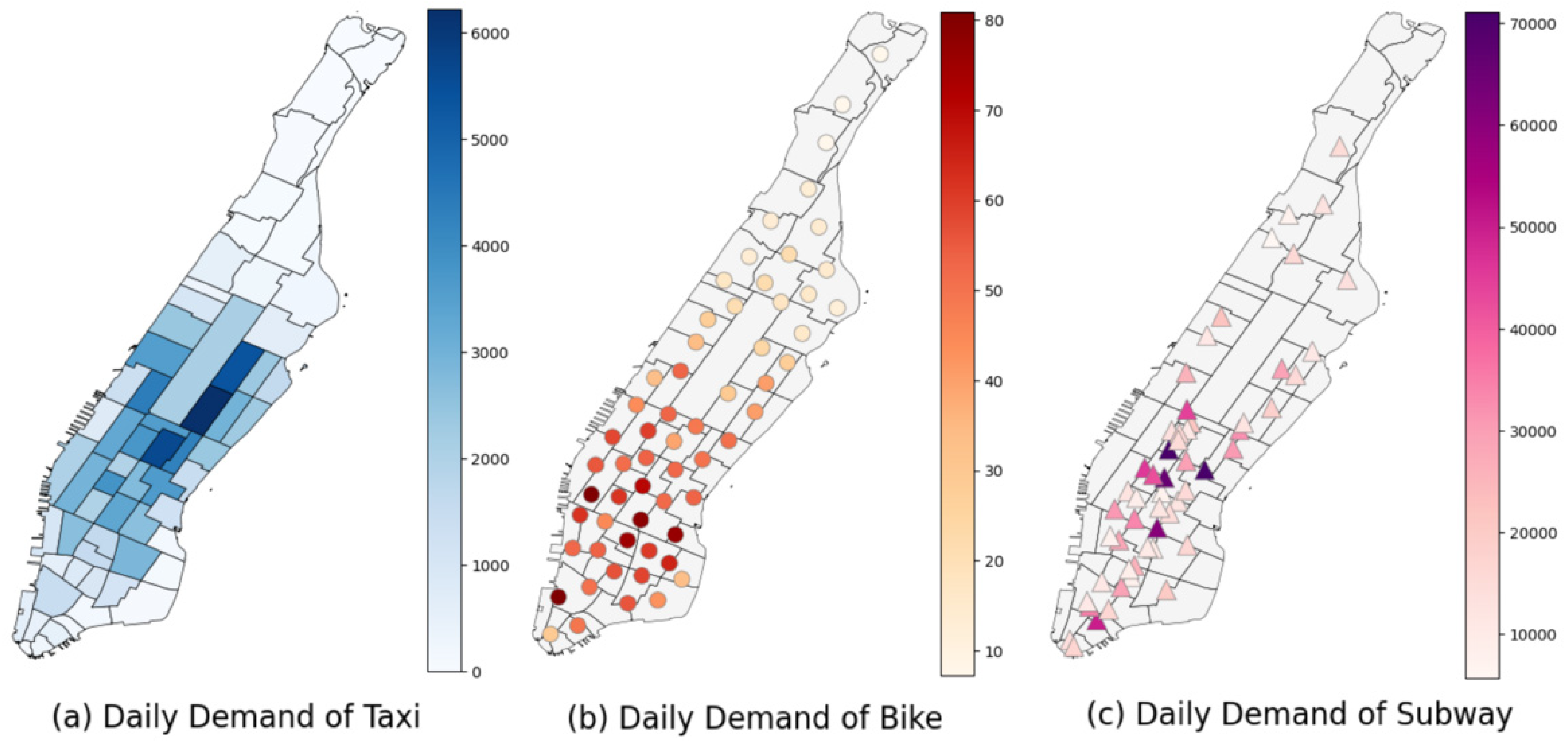
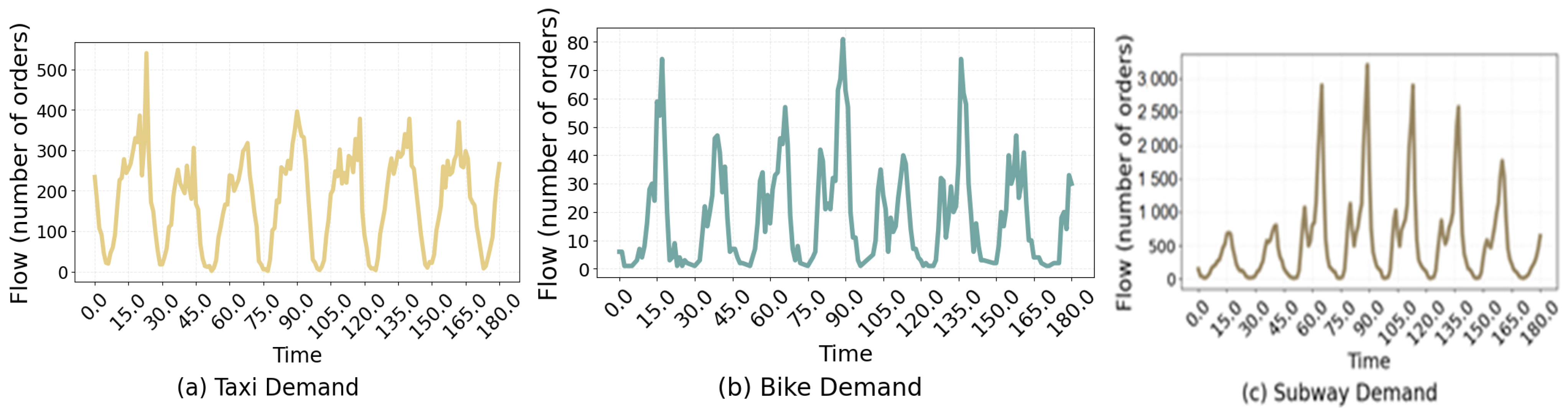
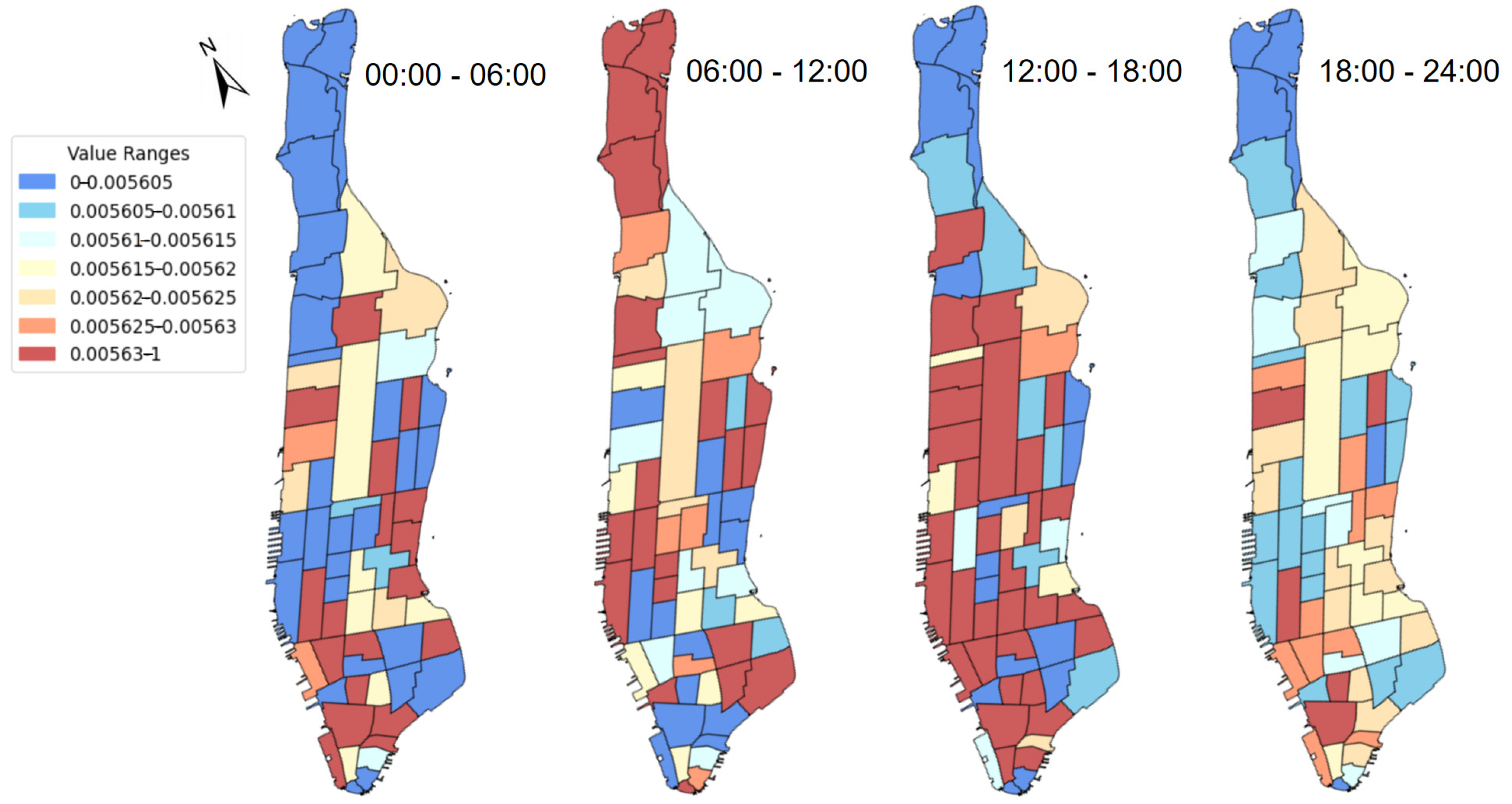
In addition, we also conducted spatiotemporal feature analysis on three types of traffic data. Figure 8 shows the spatial distribution of demand for multiple modes of transportation in New York City. It can be seen that taxi demand (a) is concentrated in the downtown commercial area, bicycle demand (b) forms hotspots in residential areas and commuting hubs, while subway demand (c) is highly concentrated in major transportation hubs, which intuitively reflects the spatial heterogeneity of multi-modal data. From the time series perspective (Figure 9), all three patterns exhibit significant periodicity (such as morning and evening peaks) and volatility. The demand for taxis fluctuates sharply and has no clear pattern; the demand for bicycles exhibits a regular short-term peak; the subway has the largest demand volume and there is a continuous peak during the day. This collectively constitutes a complex, multi-scale temporal dynamic challenge in prediction tasks.
To construct the input for the model, the raw transaction data from each mode (taxi, bike, subway) were converted into a unified 4D tensor representation X R B × T × N × D , where B is the batch size, T is the historical time steps, N is the number of spatial nodes, and D is the feature dimension. This was achieved by aggregating records into hourly departure demand counts, mapping each data point to its respective spatial unit (63 regions for taxis, 60 virtual stations for bikes, 55 physical stations for subways), and normalizing the numerical features. The key distinction between the datasets lies in the dimension N , allowing the model to handle heterogeneous spatial units within a consistent architectural framework.

5.2. Baseline Models

To validate the effectiveness of the proposed model, we compared it with various baseline models, including multi-modal prediction methods for heterogeneous spatial units, and several unimodal prediction methods. Below is a detailed introduction to each baseline model and its parameter settings.
  • HA (Historical Average): A simple time series forecasting method that predicts future demand by calculating the average of historical time steps.
  • LR (Linear Regression): A classic statistical analysis method that models the linear relationship between demand and historical time series to forecast future demand.
  • XGBoost (Extreme Gradient Boosting) [49]: A machine learning method based on a gradient boosting framework that predicts future traffic demand by constructing regression tree models.
  • LSTM (Long Short-Term Memory) [50]: A deep learning approach that serves as a variant of RNNs. LSTM captures long-term dependencies in sequences through gating mechanisms, making it suitable for time series forecasting.
  • STGCN (Spatiotemporal Graph Convolutional Network) [6]: A deep learning method based on graph neural networks that combines spectral graph convolution and temporal convolution layers to model spatial and temporal correlations.
  • DCRNN (Diffusion Convolutional Recurrent Neural Network) [51]: A spatiotemporal graph convolutional network that utilizes an encoder–decoder structure, combining graph convolution networks and GRUs to capture spatiotemporal dependencies.
  • Graph WaveNet [35]: A spatiotemporal graph learning method that performs node embedding through self-learning adjacency matrices, using temporal and graph convolutions to capture complex spatiotemporal dependencies.
  • HGNN (Hypergraph Neural Network) [14]: A deep learning approach that handles complex data structures by modeling data through hypergraph structures and performing feature learning via hypergraph convolution.
  • DHGNN (Dynamic Hypergraph Neural Network) [52]: A neural network method that models dynamically evolving hypergraph structures, adapts to data changes through dynamic updates of the hypergraph structure, and encodes high-order data relationships via vertex and hyperedge convolutions.
  • CoGNN [11]: A demand collaborative prediction method for self-learning multi-modal heterogeneous graphs, which captures relationships between heterogeneous nodes through self-learning matrices and models temporal and spatial features separately using spatiotemporal convolutional networks.
  • ST-MRGNN (Multi-Relation Spatiotemporal Graph Neural Network) [12]: A multi-modal demand collaborative prediction method for heterogeneous spatial units that captures intra- and inter-modal spatial relationships of multi-modal data through graph neural networks, employing temporal convolutional and graph convolutional layers to capture complex spatiotemporal dependencies.
  • TSHDNet (Temporal-Spatial Heterogeneity Decoupling Network) [38]: A multi-modal traffic flow prediction method separates the temporal dynamics and spatial heterogeneity within and between modes through a gated attention mechanism that employs adaptive hyperedges to capture complex spatial dependencies.

5.3. Experiment Settings

The CPU used in this experiment was an Intel Xeon E5-2650 v4, and the GPU was an NVIDIA Tesla T4, which is based on NVIDIA’s Turing architecture and features 2560 CUDA cores, supporting various computation precisions. The operating system was Windows 11, the programming language was Python, and the deep learning framework was PyTorch 1.13.1.
To ensure data quality, a rigorous preprocessing pipeline was applied before modeling. Firstly, outliers in traffic order data (e.g., travel time, speed, trip distance) beyond the 99th percentile were filtered out. Subsequently, missing values were imputed using linear interpolation, and spatiotemporal consistency checks (e.g., valid timestamps and geographical coordinates within Manhattan) were performed. To eliminate dimensional discrepancies, all numerical features were normalized to the range [0, 1] using min-max scaling. The time granularity of all cleaned datasets was standardized to one hour, covering the period from 1 April to 30 June 2023, resulting in 2184 hourly records.
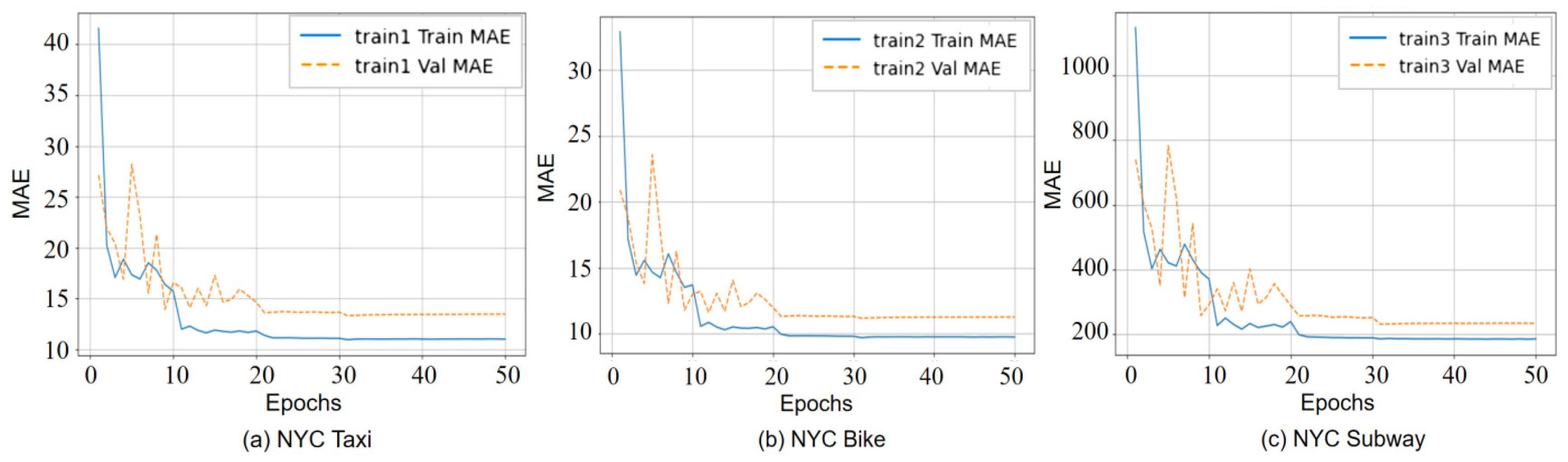
To maintain temporal integrity and prevent data leakage, the dataset was split sequentially by time into training (first 60%, April 1 to May 20), validation (next 20%, May 21 to June 10), and test (final 20%, June 11 to June 30) sets. This strategy ensures that the model is trained on historical data and evaluated on future data, mimicking real-world prediction scenarios. The validation set was utilized for model validation and hyperparameter tuning, while the test set was reserved for final evaluation. During training, we employed the Adam optimization algorithm with a cycle of 50 epochs and applied an early stopping strategy on the validation set to mitigate overfitting.
All models were evaluated on the test set using three commonly used metrics: Root Mean Square Error (RMSE), Mean Absolute Error (MAE), and Pearson Correlation Coefficient (PCC). These evaluation metrics are formally defined as follows:
R M S E = 1 n i ( y i y i ^ ) 2
M A E = 1 n i = 1 | y i ^ y i |
P C C = l = 1 n ( y i ^ y i ^ ¯ ) ( y i y i ¯ ) l = 1 n ( y i ^ y i ^ ¯ ) 2 l = 1 n ( y i y i ¯ ) 2
where n denotes the total number of samples, y i ^ represents the predicted value, and y i represents the actual value. The averages of the predicted and actual values are denoted by as y i ^ ¯ and y i ¯ , respectively.
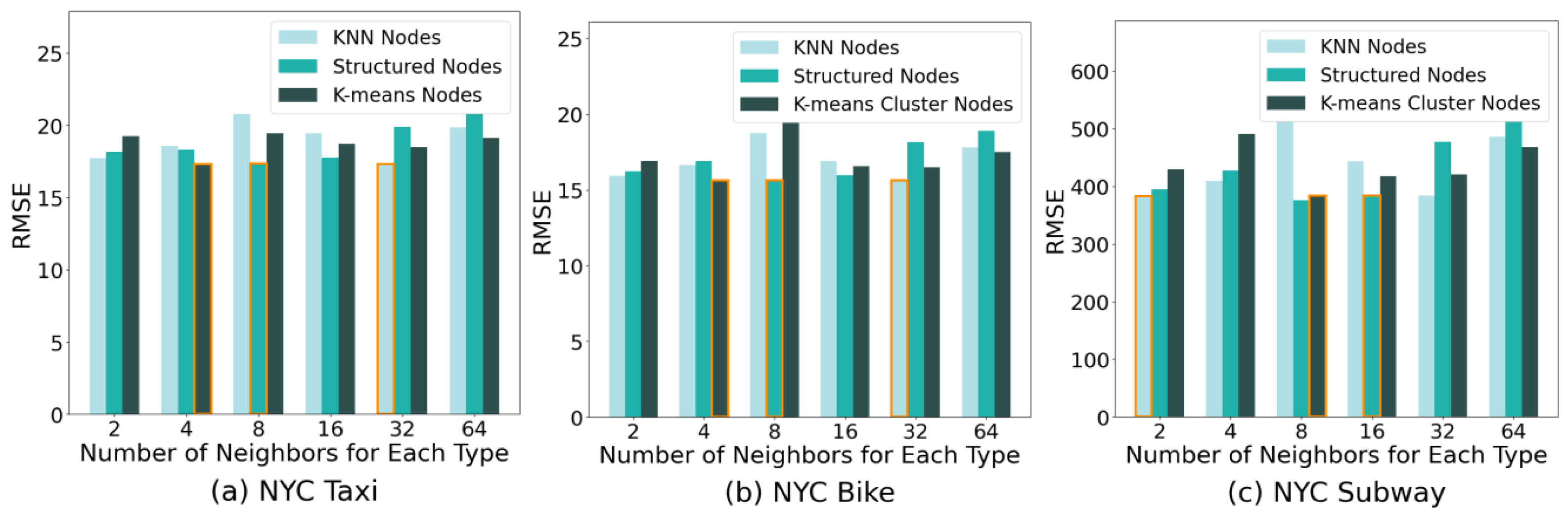
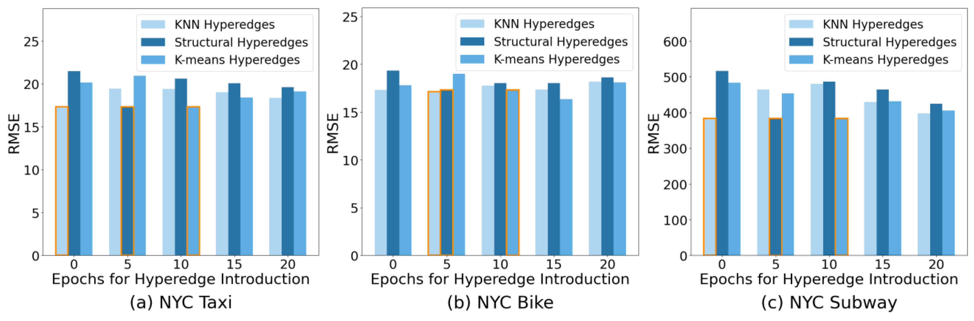
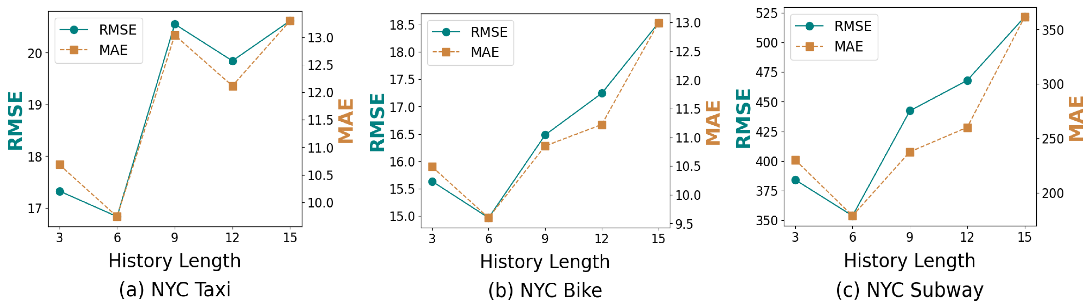
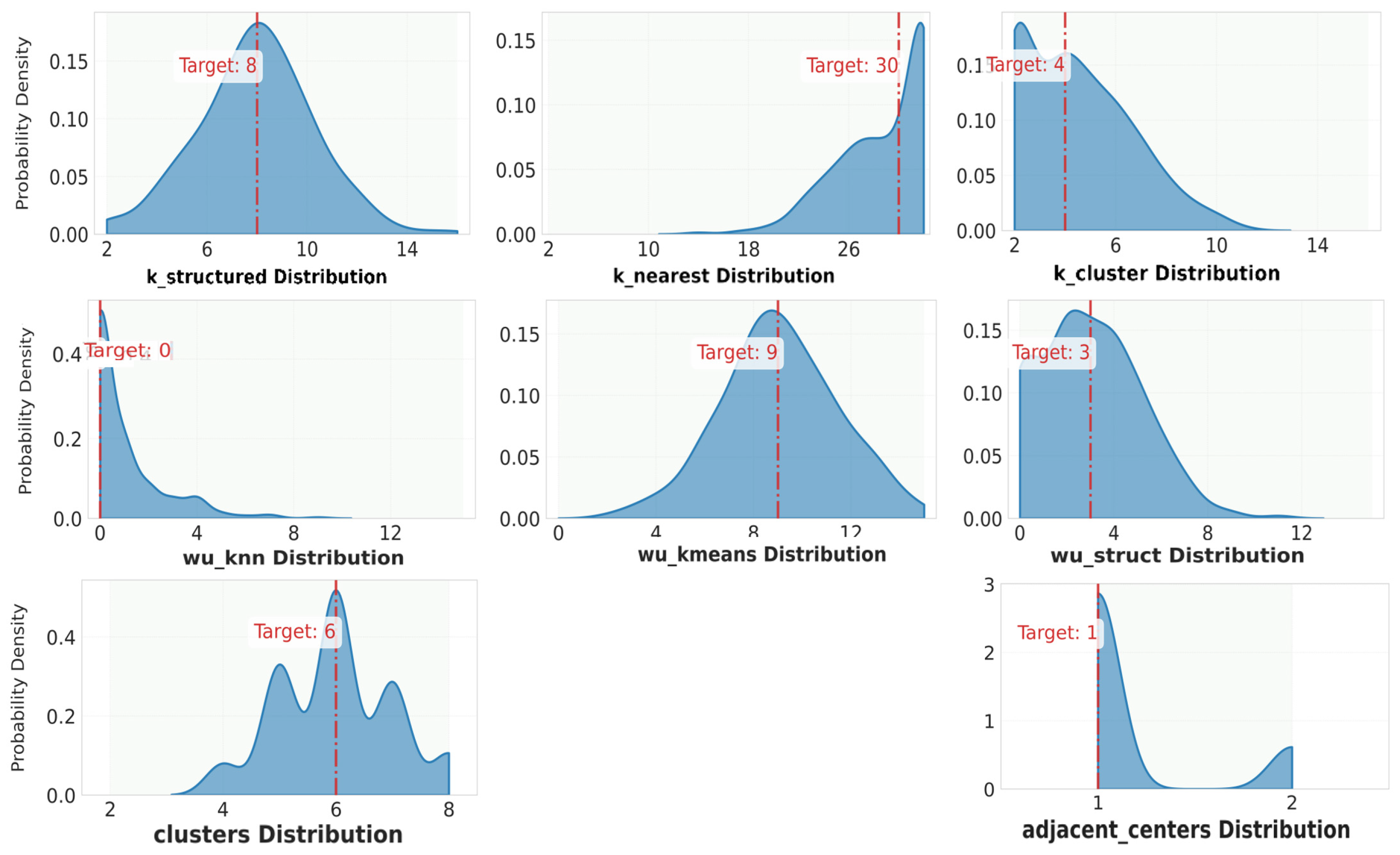
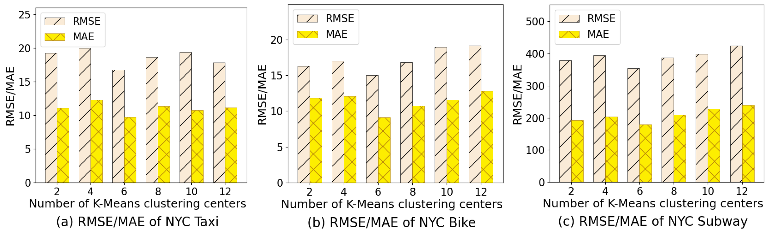
We categorized the hyperparameters into model-specific and training hyperparameters. The model hyperparameters were pertained to the architecture of MST-Hyper Trans, such as the scales and structures of the hypergraphs (e.g., the number of neighbors for different hyperedge types, the introduction epochs of various hyperedges, and the K-means clustering settings). The training hyperparameters governed the learning process, including the historical observation length, learning rate, and regularization settings. To determine the optimal values, we employed a Bayesian optimizer for model hyperparameter search, the distribution of which is illustrated in Figure 10. Subsequently, a grid search was conducted on the training hyperparameters based on the fixed model architecture. The impact of key training hyperparameters on the model’s RMSE is visualized in Figure 11 and Figure 12. Furthermore, a sensitivity analysis on the critical hyperparameters for KNN and K-means hyperedges was conducted to justify their robustness (as detailed in Appendix C). The final, optimal set of all hyperparameters for our proposed MST-Hyper Trans model is comprehensively summarized in Table 3.

5.4. Comparison of Model Performance Results

To evaluate the effectiveness of the proposed model, we conducted traffic demand prediction experiments on three traffic datasets from New York City. The experiments were divided into two parts: the first part compared single-modal demand prediction models, whereas the second part compared multi-modal demand collaborative prediction models. Table 4 presents the results of various single-modal prediction methods, while Tables 6–8 display the results of the multi-modal prediction methods under different dataset combinations. Each model was run 10 times, and the results were averaged. The best and second-best results are highlighted in bold and underlined, respectively.
As shown in the results of the single-mode experiments in Table 4, among all baseline models, the machine learning methods (HA and LR) exhibited poorer performance, whereas the performance of XGBoost in predicting the demand for shared bicycles and subways was comparable to that of LSTM. This indicates that traditional machine learning methods have limitations when handling complex spatiotemporal data. Among the single-mode deep learning methods, Graph WaveNet demonstrated superior predictive performance by capturing hidden spatial dependencies through an adaptive adjacency matrix. Both the HGNN and DHGNN achieved stable results by extracting high-order spatial dependencies through hyperedges. Our proposed MST-Hyper Trans model significantly outperformed all other baseline models across all evaluation metrics.
In the experimental results presented in Table 5, Table 6 and Table 7, MST-Hyper Trans consistently demonstrated superior predictive performance compared to CoGNN. The performance of the ST-MRGNN was relatively poor, which may be attributed to its limitations in relying on a predefined graph structure to extract spatial dependencies. In contrast, CoGNN models potential spatial information both within and between modes using an adaptive matrix, resulting in more accurate predictions. These results indicate that MST-Hyper Trans has a significant advantage in collaborative prediction for multi-modal demand. Compared to ST-MRGNN and CoGNN, MST-HyperTrans not only considers the dynamic spatial correlations among heterogeneous nodes but also effectively captures complex spatiotemporal dependencies by modeling the relationships between different traffic modes. This capability significantly enhances the predictive accuracy of the model and improves the interpretability of the inter-modal relationships. Table 8 presents a comparison of the prediction results between TSHDNet and MST-Hyper Trans across the three datasets for NYC. It is evident that MST-Hyper Trans exhibits superior predictive performance on all three datasets. This advantage may be attributed to MST-Hyper Trans’s approach of combining static and dynamic matrices for spatial dependency modeling in the transportation domain, as well as its ability to better learn the complex spatial dependencies among various traffic modes through hypergraph learning. In contrast, the predictive performance of the TSHDNet model is relatively weak, which may be due to the difficulty in capturing latent spatial information among diverse traffic modes, resulting in less accurate predictions. The results in the table indicate that MST-Hyper Trans demonstrates a more significant advantage over TSHDNet in multi-modal traffic prediction.
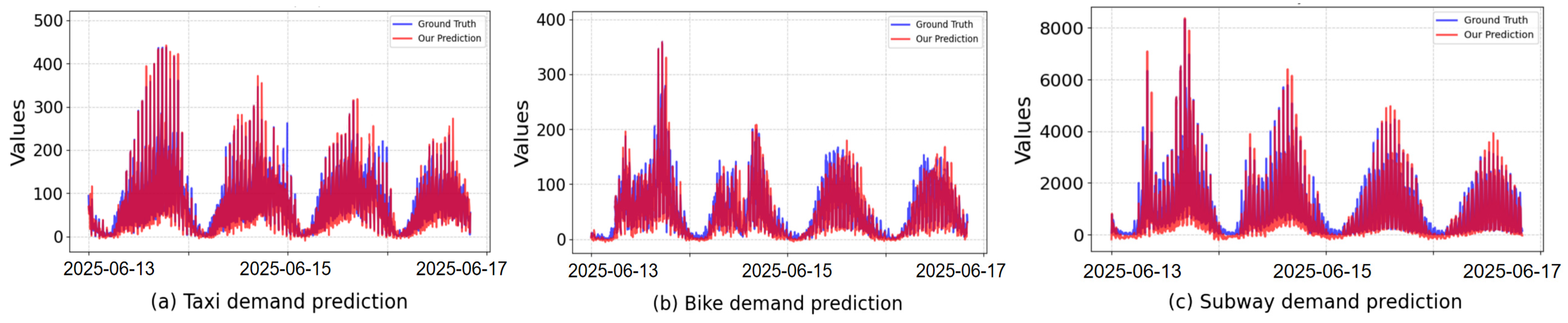
Figure 13 shows the time series comparison between the predicted and actual demand values for three transportation modes during a continuous 5-day testing period. It can be seen that our model (MST-Hyper Trans) not only has low overall error, but also accurately captures the daily cycle changes in each mode, the timing of peak occurrence and end, and the amplitude of peak values. Especially during the extreme peak days of subway demand, the model’s predicted curve closely matches the actual curve, demonstrating its ability to handle large-scale and highly fluctuating demand.

5.5. Computational Cost and Scalability Analysis

To thoroughly address the computational efficiency and scalability of the proposed MST-Hyper Trans framework, this section presents a comprehensive analysis of training/inference time, computational complexity, parameter scale, and scalability. The results demonstrate that our model achieves an optimal balance between prediction accuracy and computational overhead, confirming its practicality for real-world ITS deployments.
Firstly, there is a comparative analysis of training and inference efficiency. As summarized in Table 9 and Table 10, we compare the training time (per epoch) and inference time of MST-Hyper Trans against three representative baseline models (ST-MRGNN, CoGNN, and TSHDNet) on the NYC multi-modal dataset. The results indicate that MST-Hyper Trans achieves highly competitive efficiency: its training time per epoch is similar to ST-MRGNN and CoGNN, yet it significantly outperforms TSHDNet, which exhibits the longest training duration. More importantly, in terms of inference time, MST-Hyper Trans demonstrates superior efficiency. For instance, in the three-mode prediction task, our model achieves an inference time of 0.186 s, which is faster than TSHDNet (0.201 s) and comparable to ST-MRGNN. This efficiency is critical for real-time prediction scenarios, where a sub-second response is often required. Furthermore, when handling multiple traffic modes, the increase in both training and inference time for MST-Hyper Trans is more moderate than that of TSHDNet, highlighting its better scalability and lower computational overhead growth with increasing model complexity.
In addition, we analyze the theoretical computational complexity of MST-Hyper Trans and compare it with baseline models, as shown in Table 11. The overall time complexity of MST-Hyper Trans is O ( S · N · D · T + N · K / l o g N + N · D · H ) , and its space complexity is O ( N · D · T + N E + N D + N K + C + N 2 ) , where N is the number of nodes, D is the feature dimension, T is the time step length, S denotes the number of temporal scales, and K represents the number of neighbors in KNN. Although the theoretical complexity of MST-Hyper Trans is higher than that of lightweight models (e.g., LSTM and STGCN), it is notably lower than TSHDNet. This complexity is well justified by the model’s superior performance in capturing complex multi-modal spatiotemporal dependencies, leading to higher prediction accuracy and stronger generalization. The empirical results in Table 10 and Table 11 confirm that the theoretical complexity does not translate to prohibitive computational costs in practice, validating the model’s efficiency.
Parameter count is a critical factor affecting model computational efficiency, training stability, and deployment feasibility. As summarized in Table 12, we compare the parameter sizes of MST-Hyper Trans and baseline models. The results reveal a polarized distribution among existing models: lightweight models (e.g., CoGNN, with <10 K parameters) incur low computational overhead but lack the capacity to capture complex multi-modal spatiotemporal dependencies, while high-capacity models (such as Graph WaveNet and ST-MRGNN (>800 K parameters)) achieve higher accuracy at the cost of significantly increased training time and overfitting risk.
MST-Hyper Trans strikes an optimal balance with a total of 377 K parameters, which is comparable to STGCN (372 K) but substantially lower than Graph WaveNet and ST-MRGNN. This efficiency is achieved through the collaborative design of three modular components. This modular and dynamically adaptive design enables MST-Hyper Trans to achieve the highest prediction accuracy while maintaining computational efficiency. In the three-mode collaborative prediction task, MST-Hyper Trans requires only 4.957 s per training epoch and 0.186 s per inference, outperforming TSHDNet (5.124 s/0.201 s) and ST-MRGNN. The parameter size of 377 K thus represents a sweet spot, providing sufficient model capacity to capture complex dependencies (evidenced by an RMSE reduction of 8–11% compared to ST-MRGNN) while avoiding the computational redundancy associated with over-parameterized models.
The experimental results demonstrate that MST-Hyper Trans is highly scalable and applicable to large-scale urban networks. The model’s sub-linear growth in inference time with increasing node counts (as shown in Table 12) ensures its feasibility for metropolitan-scale deployments. For instance, in real-time traffic management systems requiring frequent updates (e.g., every 5–15 min), the inference time of 0.186 s for three modes is practically viable. Furthermore, the modular architecture allows for targeted optimization or simplification based on resource constraints, enhancing its adaptability to edge computing environments.

5.6. Ablation Analysis

To evaluate the contributions of different components in the MST-Hyper Trans model, we designed eight variants for ablation experiments. Each variant assesses the impact of specific component removal or replacement in MST-Hyper Trans on the model performance. A detailed description of each variant is provided below:
Single-scale Temporal Hyperedge (-MSTHCN_S): This variant only contains single-scale temporal hyperedge features.
No Multi-Scale Temporal Hypergraph Convolutional Network (-MSTHCN): This variant removes the MSTHCN module.
No Relationship-aware Attention Mechanism (-RAAM): This variant removes the relationship-aware attention mechanism and directly merges multiple structural hyperedges.
No Hierarchical DHGNN (-HDHGNN): This variant removes the Hierarchical DHGNN layer.
No Dynamic Spatial Hyperedge (-DMRSHN_DR): This variant removes dynamic hyperedges from the Hierarchical DHGNN layer.
No Dynamic Multi-Relation Spatial Hypergraph Network (-DMRSHN): This variant removes the DMRSHN module.
No Attention Mechanism Gating Fusion (-CMAGFN_Gate): This variant removes the gated weighted fusion in the CMAGFN module and replaces it with concatenation.
No Conditional Meta Attention Gated Fusion Network (-CMAGFN): This variant removes the CMAGFN module.
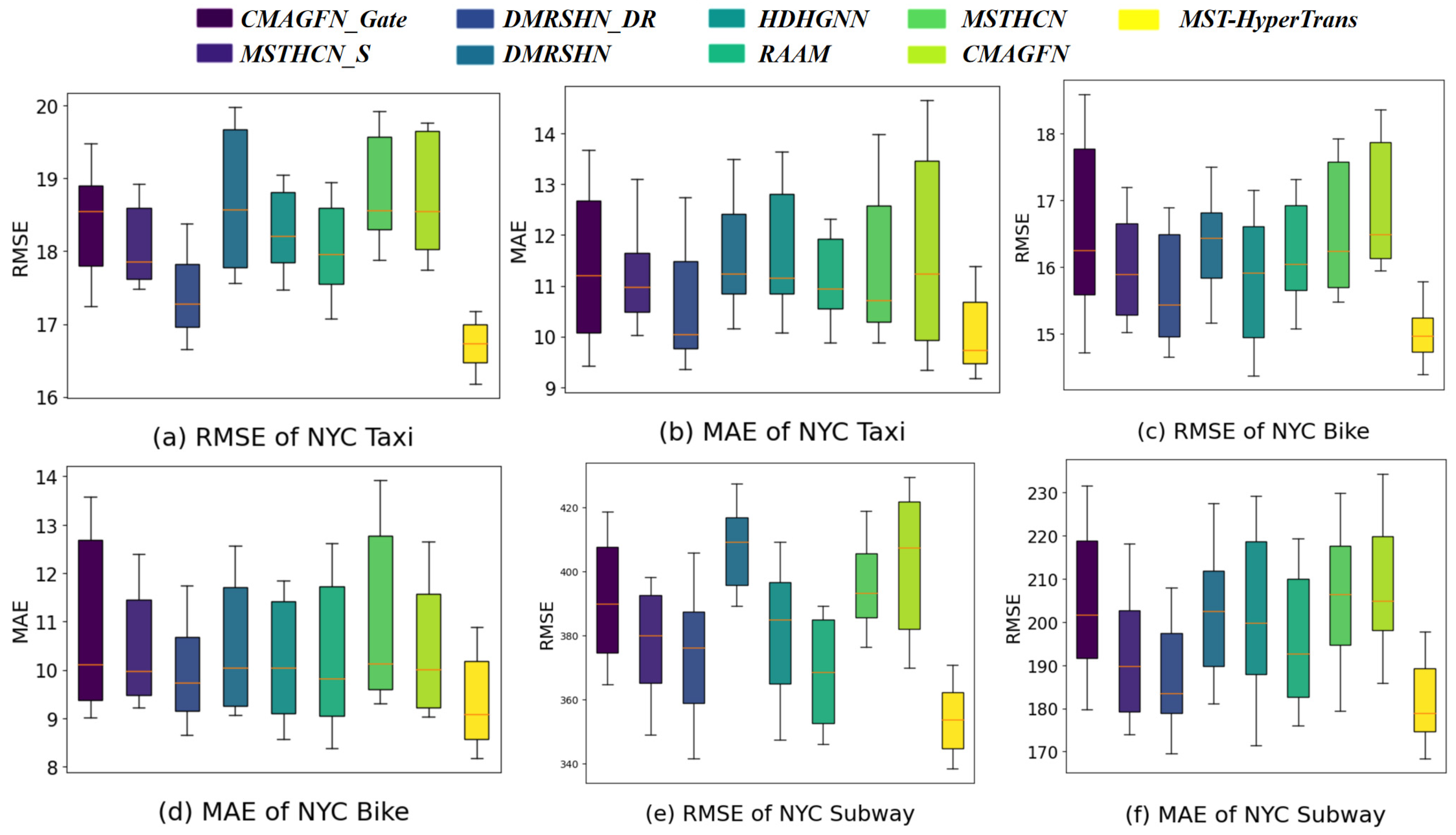
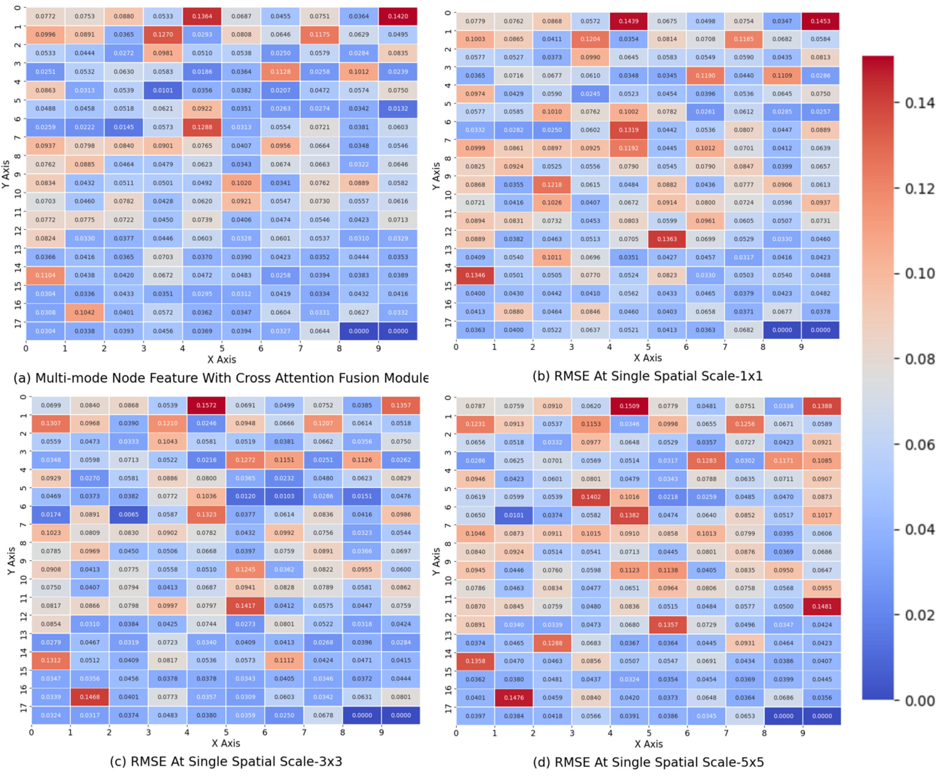
We recorded the average performance of the MST-Hyper Trans model and its variants across the three datasets after ten independent runs, as summarized in Table 13. Evaluated using the RMSE and MAE metrics, the results demonstrate that MST-Hyper Trans outperforms all its variants on each dataset, confirming the effectiveness of the model components. Specifically, the variant -DMRSHN, which excludes the Dynamic Multi-Relation Spatial Hypergraph Network (DMRSHN), shows the most significant decline in performance, exhibiting the highest RMSE and MAE values. Removing the DMRSHN module resulted in the most significant performance degradation, which confirms that dynamic multi-relational space modeling is the most critical step in multi-modal prediction tasks. In addition to DMRSHN, the variant that excludes the Conditional Meta Attention Gated Fusion Network (CMAGFN) module also significantly impacts performance, indicating that dynamically extracting various spatial relationships is crucial for modeling the complex dependencies among heterogeneous spatial units in a multi-modal context. To assess the stability of the model, we conducted a box plot analysis of the experimental results for MST-Hyper Trans and its eight variant models. Figure 14 shows the results for the NYC-Taxi, NYC-Bike, and NYC-Subway datasets. Box plots visually illustrate the data distribution characteristics through a five-number summary (maximum, minimum, median, and upper and lower quartiles). The results indicate that MST-Hyper Trans consistently exhibits lower prediction errors across the three datasets compared with all variant models, with smaller variance, suggesting higher stability and predictive accuracy.

5.7. Comparison of Multi-Traffic Modes and Single-Traffic Mode

To analyze the impact of inter-modal relationships on the predictive performance of multi-modal demand collaborative forecasting, we conducted multiple experiments on three transportation datasets from New York City using the MST-Hyper Trans model. The experimental design is as follows:
Group I: Individual predictions for taxi, subway, and bike-sharing modes.
Group II: Collaborative predictions for taxi and subway modes, with bike-sharing mode predicted separately.
Group III: Collaborative predictions for taxi and bike-sharing modes, with subway mode predicted separately.
Group IV: Collaborative predictions for subway and bike-sharing modes, with the taxi mode predicted separately.
Group V: Simultaneous collaborative predictions for taxi, subway, and bike-sharing modes, with separate output for each prediction.
Table 14 summarizes the model performance comparisons across different dataset combinations, with colored numbers indicating independent predictions for each mode within the corresponding combination. The best results for each column are highlighted in bold font. By comparing the results of different combinations, we found that the best performance was never observed in the combination in which all modes were predicted independently (Group I). This indicates that integrating data from multiple transportation modes into a single model can significantly enhance the model’s ability to learn from demand fluctuations, thereby improving prediction accuracy. From the distribution of the best results, it is evident that the majority of the optimal outcomes originated from the collaborative prediction of all three transportation modes in Group V, whereas some of the best results came from the combined predictions of bike-sharing and subway modes (Group III). This may be attributed to the low cost of bike-sharing and subway services, whereby the passenger demand exhibits similar temporal variations. Consequently, considering the correlations between the different transportation modes during collaborative forecasting is crucial for feature extraction and model learning.

5.8. Analysis of Cross-Modal Multi-Scale Spatiotemporal Relationships

To explore cross-modal multi-scale spatiotemporal dependencies, we analyzed the attention weights for the spatiotemporal dependency features captured by our method across various modes and within each mode. First, we visualized the spatiotemporal distribution of attention weights for inter-modal features at different time scales, as shown in Figure 15. The shade of the color reflects the magnitude of the attention weights. It is evident that the three traffic modes are most significantly influenced by cross-modal features at the 7 × 24 super edge (hourly) time scale, with most stations/regions exhibiting attention weights above 0.5, and many stations/regions exceeding 0.8. This indicates that cross-modal features effectively capture the spatiotemporal dependencies between traffic modes on an hourly time scale. In contrast, at the 7 × 6 super edge (four-hour) time scale, the influence of cross-modal features on nodes is significantly weakened, with node demand predictions relying more on intra-modal demand characteristics.
Subsequently, we present a heatmap of the RMSE obtained from the MST-Hyper Trans model operating at multi-spatial scales compared to a single spatial scale, as shown in Figure 16. Figure 16a illustrates the performance of our model at multi-spatial scales, while Figure 16b–d show the results of the model variants operating under three distinct single spatial scales. The color intensity in the figures reflects the range of the RMSE values under different spatial scale models. From the color distribution, it can be observed that the predictive accuracy of the model is higher under multi-spatial scales, whereas the performance of the model variants with three single convolution kernels is somewhat poorer. This indicates that the multi-spatial scale approach better captures the local and global spatial correlations among multi-modal traffic nodes, facilitating more accurate collaborative demand predictions for multiple modes.
To assess the improvement in capturing the complex spatiotemporal dependencies among various transportation modes at multiple spatiotemporal scales, we visualized the spatial distribution of the RMSE improvement ratios of the spatiotemporal multi-scale MST-Hyper Trans model compared to the single spatiotemporal scale MST-Hyper Trans model under different transportation modes. The RMSE improvement distribution for the three transportation modes is illustrated in Figure 17. The color intensity in the figure reflects the RMSE improvement ratios in different regions under spatiotemporal multi-scale modeling. From the color distribution, it can be observed that the prediction accuracy of nodes for all three transportation modes generally improved under multi-temporal scale modeling. The taxi mode exhibited the most significant enhancement in prediction accuracy, with many regions showing RMSE improvement ratios that exceeded 16%. Furthermore, in areas with lower subway network coverage, spatiotemporal multi-scale modeling notably improves the prediction accuracy for shared bicycles. This indicates that in regions with lower demand or weaker inter-mode dependencies, the extraction of multi-temporal scale features can better compensate for the shortcomings of single temporal scale modeling.

5.9. Analysis of Information Interaction Mechanism Between Multi-Modes

To explore the information interaction mechanisms among multiple transportation modes, we conducted a heatmap analysis of the attention gating vector changes in the cross-modal spatiotemporal features and intra-modal node features within the CMAGFN module across different time periods of the day. The results are shown in Figure 18. Throughout the day, the influence of cross-modal spatiotemporal features on the demand for multi-modal transportation varies with time. Notably, during the time periods of 00:00–06:00 and 18:00–24:00, the weight of the cross-modal spatiotemporal features is at its peak.
To further investigate the spatial characteristics of cross-modal spatiotemporal information interaction mechanisms, we performed a visual analysis of the attention gating of intra-modal node features for taxi nodes within the CMAGFN module in the Manhattan area, focusing on four key time periods throughout the day (Figure 19). Analysis combined with Points of Interest (POI) information in the Manhattan area reveals that during most parts of the day, the proportion of cross-modal spatiotemporal information is relatively high in the Upper Manhattan area. This was attributed to the presence of numerous luxury apartments and villas, resulting in sparse demand data across the three transportation modes, thereby highlighting the significance of cross-modal spatiotemporal information. In contrast, for the Financial District, during weekday daytime hours (e.g., 06:00–18:00), the traffic volume is substantial, leading to a relatively minor impact of cross-modal spatiotemporal information on transportation demand. However, at night, the traffic volume in the Financial District decreases significantly, which subsequently enhances the importance of cross-modal spatiotemporal information.

6. Conclusions

This study addresses the core challenges in multi-modal transportation demand forecasting, namely the coexistence of heterogeneous spatial units (e.g., taxi zones, bicycle stations, and subway stations) and the complex spatiotemporal dynamics inherent in urban traffic systems. To this end, the Multi-Scale Spatiotemporal Dynamic Hypergraph Convolutional Network (MST-Hyper Trans) is proposed. The model achieves accurate and dynamic modeling of high-order spatiotemporal dependencies through the integration of three core modules: the Multi-scale Temporal Hypergraph Convolutional Network (MSTHCN) for temporal pattern decoupling, the Dynamic Multi-Relationship Spatial Hypergraph Network (DMRSHN) for spatial correlation capture, and the Conditional Meta Attention Gated Fusion Network (CMAGFN) for adaptive feature fusion. Experimental results on multi-modal NYC data demonstrate that the proposed model achieves an average improvement of 9.07% in PCC and reduces RMSE by 7.6% compared to state-of-the-art benchmarks, validating its superior accuracy.
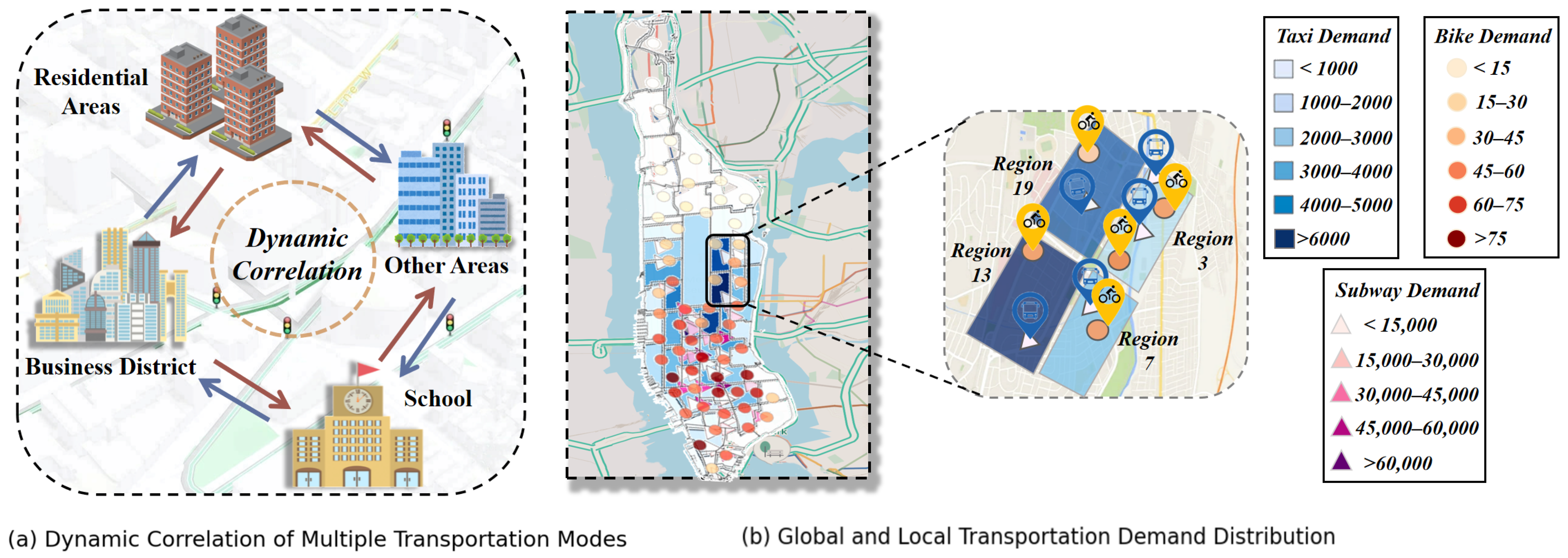
Unlike traditional methods reliant on static graphs, the MST-Hyper Trans framework incorporates geographic proximity, passenger flow similarity, and transportation connectivity to construct structural hyperedges, while employing KNN and K-means algorithms to generate dynamic hyperedges. This approach overcomes the limitations of ordinary graph models in capturing multi-node relationships and explicitly models the evolution of spatial dependencies with traffic conditions. By decoupling multi-time scale (e.g., hourly, daily, weekly) patterns via MSTHCN and hierarchically extracting local-to-global spatial features via DMRSHN, the model characterizes spatiotemporal traffic characteristics more effectively. The CMAGFN module further enhances this by leveraging a lightweight meta-network with multi-head cross-attention to dynamically calibrate fusion weights based on real-time context (e.g., time, weather, and demand), enabling context-aware decision-making and improving prediction accuracy and interpretability.
Experimental validation on real-world datasets from New York City demonstrates the superior predictive accuracy of MST-Hyper Trans. For instance, on the NYC-Taxi dataset, it attained an RMSE of 16.51 and an MAE of 9.63, which are 10.6% and 14.23% lower, respectively, than the CoGNN baseline. Similar improvements were observed across all modes. Ablation studies confirm the indispensable contributions of each module, and case analyses reveal physically meaningful cross-modal interactions (e.g., subway–bicycle demand connections during peak hours), offering actionable insights for resource allocation and scheduling. While the model exhibits superior performance, future work will focus on integrating richer external data (e.g., refined weather, social events, and road dynamics) to enhance scalability in complex scenarios.

Author Contributions

J.C.: conceptualization, formal analysis, project administration, writing—original draft, writing—review and editing; M.S.: data curation, formal analysis, methodology, visualization, writing—original draft, writing—review and editing. All authors have read and agreed to the published version of the manuscript.

Funding

Thanks for the support of the National Natural Science Foundation of China project (61104166).

Institutional Review Board Statement

Not applicable.

Informed Consent Statement

Not applicable.

Data Availability Statement

The traffic data used in this study can be obtained from the public data platform of New York City, the taxi historical order data can be obtained through TLC Trip Record Data—TLC, the subway historical card reading data can be obtained from MTA Subway Hourly Ridership: 2020–2024|State of New York, and the bike historical order data can be obtained from Index of bucket “tripdata”.

Conflicts of Interest

The authors declare no conflicts of interest.

Appendix A

To assist readers in better understanding the symbols and their definitions used in this paper, we have compiled all key symbols along with their meanings in tabular form. Table A1 lists the main symbols defined in this study, their specific definitions, and their corresponding meanings in English.
Table A1. Summary of notations used in this paper.
NotationDescriptionUnits
M i Set of nodes for the i -th transportation modecount
M Entire set of nodes for all transportation modescount
r Number of transportation modes in the systemcount
n Number of nodes in a transportation modecount
ν Set of traffic nodes (stations or regions) in the urban transportation system.count
ν m Set of nodes for the m -th traffic mode.count
ε Set of edges representing relationships between nodes.count
G Heterogeneous transportation graphdimensionless
G M i Intra-modal relation graph for the i -th transportation modedimensionless
G M i j Inter-modal relation graph between M i and M j dimensionless
C E External factor Featurevaries
x i ( t ) Transportation demand at node i during time step t passengers/hour
X M i ( t ) Feature matrix of nodes for the i -th transportation mode at time tpassengers/hour
A M i Weighted adjacency matrix for intra-modal relationsdimensionless
A M i j Weighted adjacency matrix for inter-modal relationsdimensionless
H e Hyperedge set on hypergraph structurecount
H u Node set on hypergraph structurecount
Z M S T H C N Features captured by MSTHCN modulesdimensionless
Z i n t e r _ S T Features captured by DMRSHN modulesdimensionless
L Length of historical time steps used for predictionhours (h)
F ( · ) Mapping function to predict future demanddimensionless
x i f i n a l Predicted transportation demand at node i -thpassengers/hour
X T + 1 Predicted transportation demand at time T + 1 passengers/hour
d ( v ) Degree of vertex ν in a hypergraphcount
δ ( e ) Degree of hyperedge e count
Δ i n Intra-modal hypergraph Laplacian operatordimensionless
Δ i n t e r Inter-modal hypergraph Laplacian operatordimensionless
Φ Orthogonal eigenvectors of the Laplacian matrixdimensionless
Λ Diagonal matrix of eigenvaluesdimensionless
Θ Trainable parameter matrix in hypergraph convolutiondimensionless
σ Activation function (e.g., ReLU, Sigmoid)dimensionless
gThe gating vector of CMAGFN moduledimensionless
ω Weight of hyperedgedimensionless
DSCSørensen–Dice coefficient for hyperedge mergingdimensionless
MLPMulti-layer perceptrondimensionless
SoftmaxSoftmax activation functiondimensionless
ReLURectified Linear Unit activation functiondimensionless
ConcatConcatenation operationdimensionless
LayerNormLayer normalizationdimensionless
FeedForwardFeed-forward neural networkdimensionless
[ · · ] The splicing operationdimensionless
γ Weight of L2 regularization termdimensionless
ϵ m Loss weight for mode m dimensionless
k N N Number of neighbors in KNN hyperedge constructioncount
k c Number of clusters in K-means hyperedge constructioncount
k s Number of neighbors in Structure hyperedge constructioncount
L M Number of MDHGNN Layerscount
α Attention weight for fusing time and space features.dimensionless
sNode level attention scores based on different structural featuresdimensionless
β Attention weight for fusing features from different viewsdimensionless

Appendix B

Algorithm A1 outlines the process of the DMRSHN module.
Algorithm A1: The process of DMRSHN Layer
Input: historical demand data X T L : T = { X M i T L : T , M i } , number of MDHGNN layers L , output of MSTHCN layer Z M S T H C N
Parameter: Number of structural hyperedges K s t r , Number of KNN hyperedges K n n , Number of K-Means hyperedges K c l u s t e r , Number of Cluster Centers n c l u s t e r , Number of adjacent cluster centers n c e n t e r
Output: Extracted spatial-temporal features X T R D R
Initialize the parameters of DMRSHN Layer;
For i { 1,2 , N } do
  Build primary Geographic distance Graph M G R N × N , Passenger flow similarity Graph M P R N × N , and Connection relationship Graph M C R N × N ;
  Build three type structural hyperedge H G , H P , H C R N × K s t r ;
  Compute X G , X P , X C from a HGNN layer given H G , H P , H C , X T L : T ;
  Calculate the weight of relationship-aware attention and fuse it with weighted weights to obtain Z s p a t i a l ;
  Initialize Z s p a t i a l as X S ;
  Identify the nearest k neighbors of each feature point using KNN;
  Build KNN hyperedge H N N R N × K n n ;
  Cluster node features into n c l u s t e r classes using K-Means;
  Select neighboring nodes on the top n c e n t e r cluster centers for each node;
  Construct K-Means hyperedge H K M e a n s R N × K c l u s t e r ;
  Compute Z i n t e r _ S T from hierarchical hypergraph convolution layer given Z M S T H C N , H N N , H K M e a n s ;
End

Appendix C

To ensure the robustness of the proposed dynamic hyperedge generation mechanism and provide empirical evidence for the selection of key hyperparameters, we conducted a systematic sensitivity analysis. Specifically, we evaluated the following: (1) Number of KNN neighbor nodes: As shown in Figure A1, we tested the impact of varying the number of neighbors for three relationships (KNN, structured, K-means clustering) from 2 to 64 on RMSE on three NYC datasets. The results showed that the model performance remained relatively stable over a wide range of parameters (with small RMSE fluctuations), and reached the optimal or near-optimal equilibrium point on most datasets when the number of KNN neighbors was 32, confirming the model’s insensitivity to this parameter. (2) Timing of introducing hyperedges: As shown in Figure A2, we investigated the impact of introducing three types of relation hyperedges at different training epochs (Epoch) on RMSE. Experiments have shown that dynamic introduction strategies (such as K-means hyperedges introduced in the 10th round) can bring better or comparable model convergence and final performance compared to initial introduction. The orange lines in Figure A1 and Figure A2 represent the hyperparameter values at which the optimal results are obtained. (3) K-means clustering center count: As shown in Figure A3, we analyzed the impact of varying the number of clustering centers from 2 to 12 on RMSE and MAE in different datasets. The results showed that when the number of cluster centers was set to 6, the model achieved optimal or near-optimal prediction errors on all three datasets, and this value was determined as the best choice that balances the model’s expressive ability and generalization ability. These sensitivity analyses collectively validated the robustness of the dynamic hyperedge mechanism to parameter perturbations and provided direct support for the final parameter settings.
Figure A1. The impact of three types of neighbor node numbers on RMSE under different NYC datasets.
Futuretransp 06 00051 g0a1
Figure A2. The impact of introducing three types of relationship hyperedges on RMSE at different epochs in different NYC datasets.
Futuretransp 06 00051 g0a2
Figure A3. The impact of the number of cluster centers on the RMSE of different datasets.
Futuretransp 06 00051 g0a3

References

  1. Jabbarpour, M.R.; Zarrabi, H.; Khokhar, R.H.; Shamshirband, S.; Choo, K.-K.R. Applications of Computational Intelligence in Vehicle Traffic Congestion Problem: A Survey. Soft Comput. 2018, 22, 2299–2320. [Google Scholar] [CrossRef]
  2. Yang, Y.; Lu, H. Short-Term Traffic Flow Combined Forecasting Model Based on SVM. In Proceedings of the 2010 International Conference on Computational and Information Sciences, Chengdu, China, 17–19 December 2010; IEEE: New York, NY, USA, 2011; pp. 262–265. [Google Scholar]
  3. Yu, J.W.; Jang, J.E. A Kalman Filter Ramp Traffic Forecasting Model for Real-Time Traffic Control and Information Provision. 2009. Available online: https://www.google.com/url?sa=t&source=web&rct=j&opi=89978449&url=https://www.jstage.jst.go.jp/article/eastpro/2011/0/2011_0_101/_pdf&ved=2ahUKEwjC0cCunPGSAxXGha8BHWcqAZMQFnoECCEQAQ&usg=AOvVaw11buHgfTmtM3aDq824xE8E (accessed on 17 February 2026).
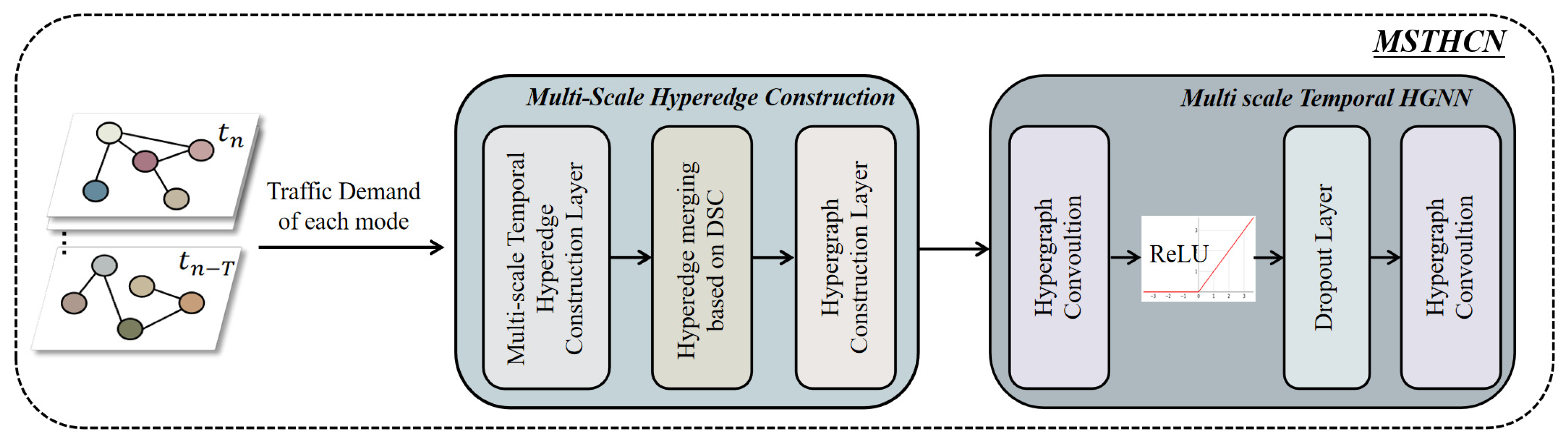
  4. Chaudhry, A.; Li, W.; Basri, A.; Patenaude, F. A Method for Improving Imputation and Prediction Accuracy of Highly Seasonal Univariate Data with Large Periods of Missingness. Wirel. Commun. Mob. Comput. 2019, 2019, 1–13. [Google Scholar] [CrossRef]
  5. Li, Y.; Yu, R.; Shahabi, C.; Liu, Y. Diffusion Convolutional Recurrent Neural Network: Data-Driven Traffic Forecasting. arXiv 2018, arXiv:1707.01926. [Google Scholar] [CrossRef]
  6. Yu, B.; Yin, H.; Zhu, Z. Spatio-Temporal Graph Convolutional Networks: A Deep Learning Framework for Traffic Forecasting. In Proceedings of the Twenty-Seventh International Joint Conference on Artificial Intelligence, Stockholm, Sweden, 13–19 July 2018; pp. 3634–3640. [Google Scholar]
  7. Bai, L.; Yao, L.; Li, C. Adaptive Graph Convolutional Recurrent Network for Traffic Forecasting. arXiv 2020, arXiv:2007.02842. [Google Scholar] [CrossRef]
  8. Li, R.; Zhong, T.; Jiang, X.; Trajcevski, G.; Wu, J.; Zhou, F. Mining Spatio-Temporal Relations via Self-Paced Graph Contrastive Learning. In Proceedings of the 28th ACM SIGKDD Conference on Knowledge Discovery and Data Mining, Washington, DC, USA, 14 August 2022; ACM: Singapore, 2022; pp. 936–944. [Google Scholar]
  9. Shao, Z.; Zhang, Z.; Wei, W.; Wang, F.; Xu, Y.; Cao, X.; Jensen, C.S. Decoupled Dynamic Spatial-Temporal Graph Neural Network for Traffic Forecasting. arXiv 2022, arXiv:2206.09112. [Google Scholar] [CrossRef]
  10. Huang, X.; Ye, Y.; Ding, W.; Yang, X.; Xiong, L. Multi-Mode Dynamic Residual Graph Convolution Network for Traffic Flow Prediction. Inf. Sci. 2022, 609, 548–564. [Google Scholar] [CrossRef]
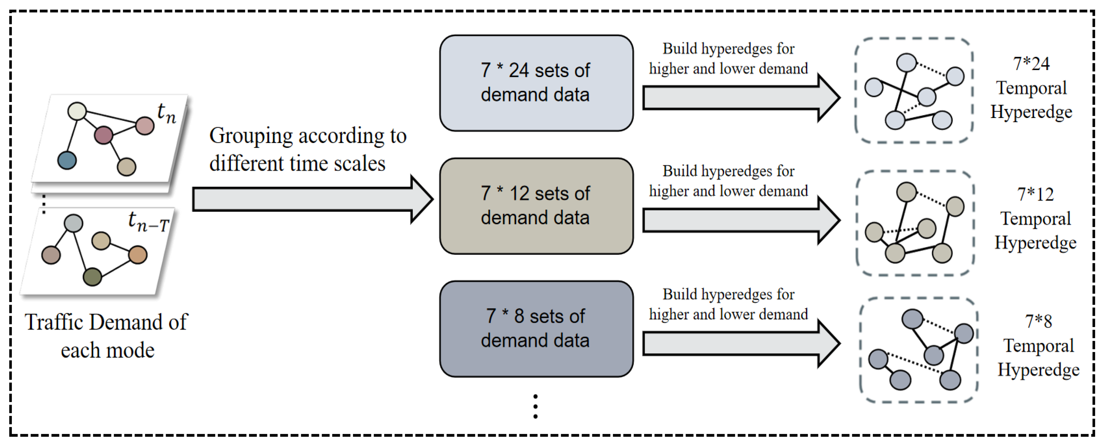
  11. Liu, M.; Du, B.; Sun, L. Co-Prediction of Multimodal Transportation Demands with Self-Learned Spatial Dependence. In Proceedings of the 2021 IEEE International Conference on Big Data (Big Data), Orlando, FL, USA, 15 December 2021; IEEE: New York, NY, USA, 2021; pp. 824–833. [Google Scholar]
  12. Liang, Y.; Huang, G.; Zhao, Z. Joint Demand Prediction for Multimodal Systems: A Multi-Task Multi-Relational Spatiotemporal Graph Neural Network Approach. Transp. Res. Part C 2022, 140, 103731. [Google Scholar] [CrossRef]
  13. Lea, C.; Flynn, M.D.; Vidal, R.; Reiter, A.; Hager, G.D. Temporal Convolutional Networks for Action Segmentation and Detection. In Proceedings of the 2017 IEEE Conference on Computer Vision and Pattern Recognition (CVPR), Honolulu, HI, USA, 21–26 July 2017; IEEE: New York, NY, USA, 2017; pp. 1003–1012. [Google Scholar]
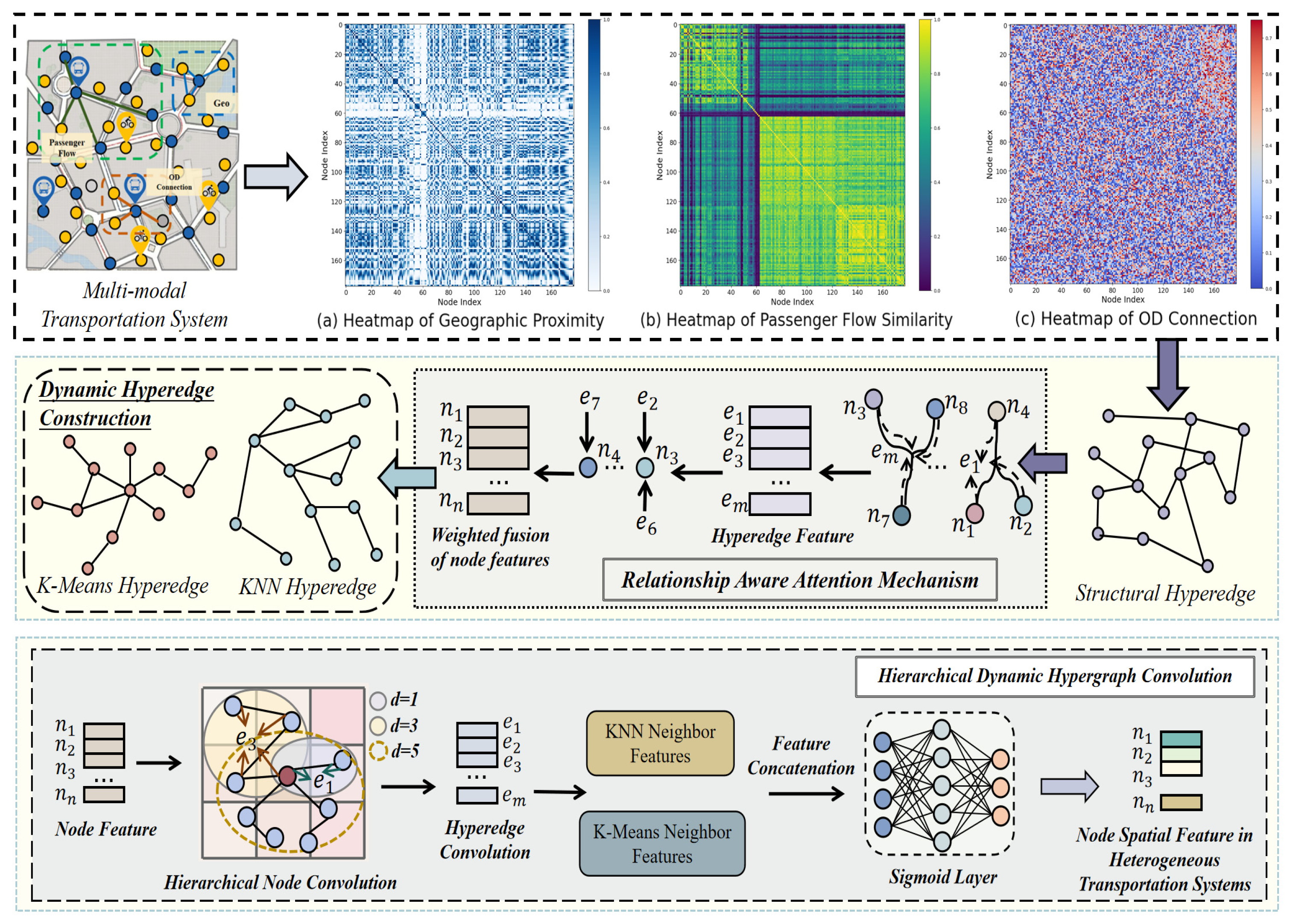
  14. Feng, Y.; You, H.; Zhang, Z.; Ji, R.; Gao, Y. Hypergraph Neural Networks. AAAI 2019, 33, 3558–3565. [Google Scholar] [CrossRef]
  15. Wang, J.; Zhang, Y.; Wei, Y.; Hu, Y.; Piao, X.; Yin, B. Metro Passenger Flow Prediction via Dynamic Hypergraph Convolution Networks. IEEE Trans. Intell. Transport. Syst. 2021, 22, 7891–7903. [Google Scholar] [CrossRef]
  16. Zhao, Y.; Ding, F.; Tan, H. Attention-Based Local-Global Hypergraph Convolutional Network for Traffic Flow Forecasting. In Proceedings of the CICTP 2024, Shenzhen, China, 11 December 2024; American Society of Civil Engineers: Reston, VA, USA, 2024; pp. 1643–1653. [Google Scholar]
  17. Ye, Z.; Wang, H.; Przystupa, K.; Majewski, J.; Hots, N.; Su, J. Dynamic Spatio-Temporal Hypergraph Convolutional Network for Traffic Flow Forecasting. Electronics 2024, 13, 4435. [Google Scholar] [CrossRef]
  18. Cao, S.; Wu, L.; Zhang, R.; Chen, Y.; Li, J.; Liu, Q. A Spatial-Temporal Gated Hypergraph Convolution Network for Traffic Prediction. IEEE Trans. Veh. Technol. 2024, 73, 9546–9559. [Google Scholar] [CrossRef]
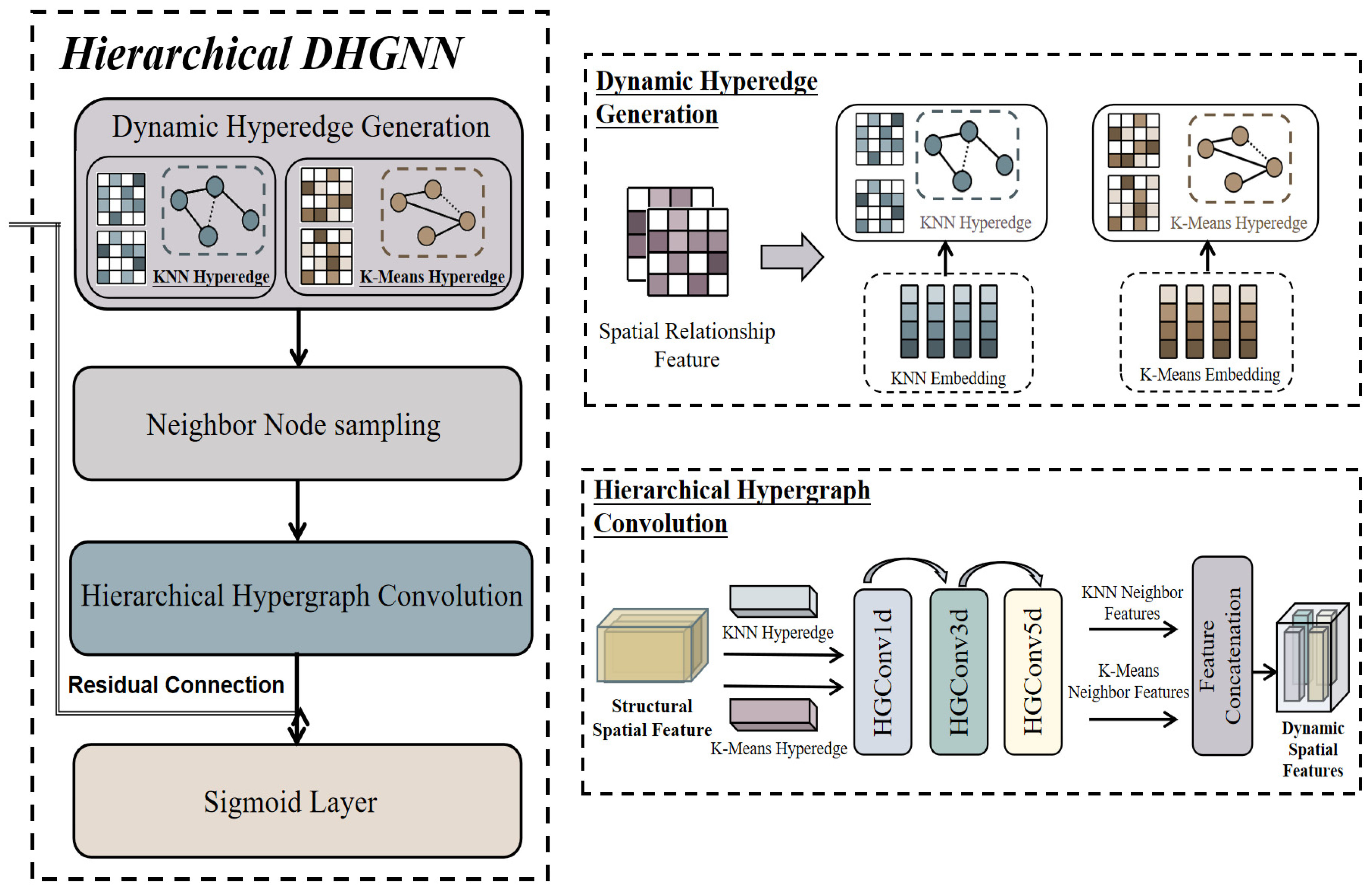
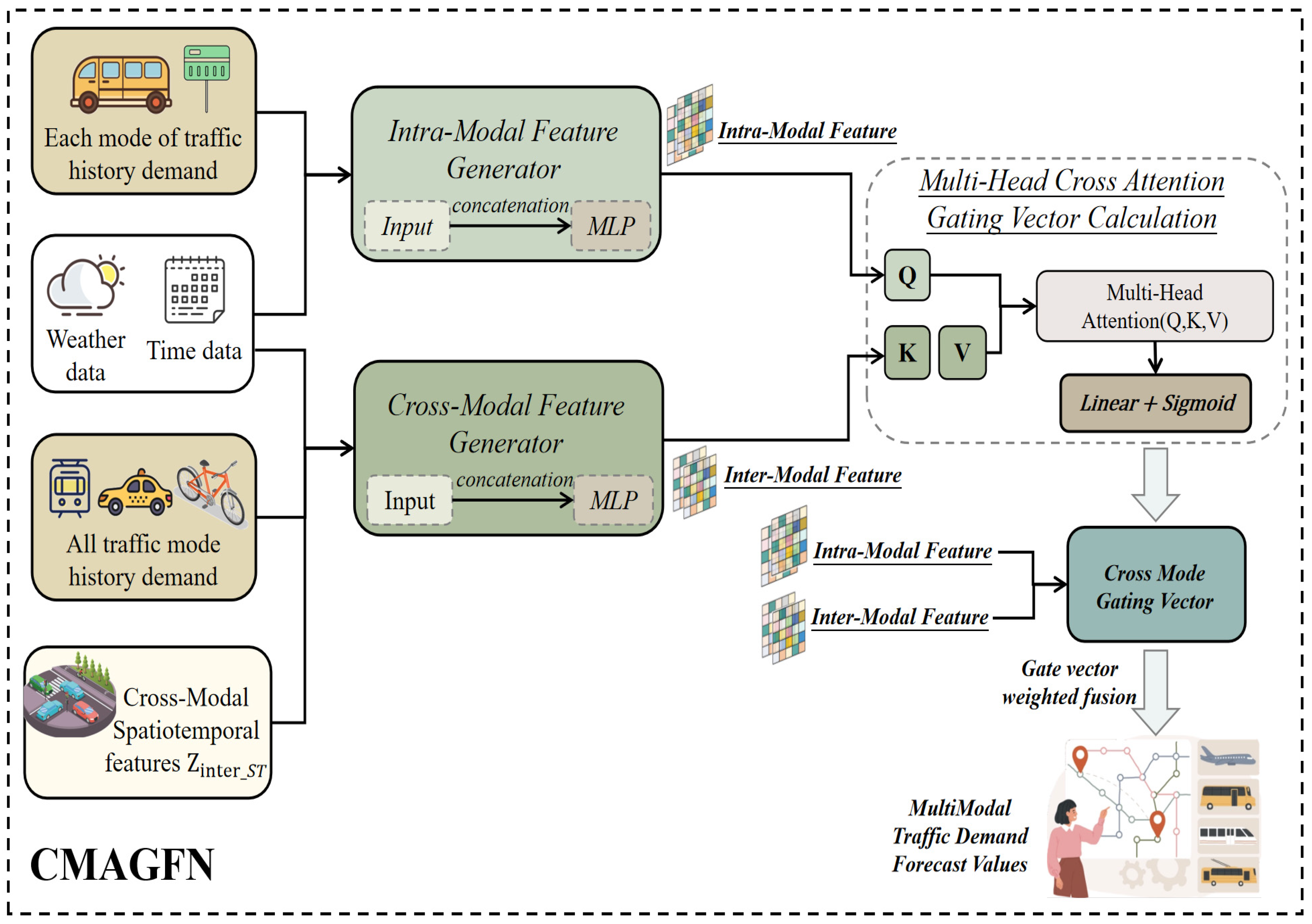
  19. Ma, X.; Zhang, J.; Du, B.; Ding, C.; Sun, L. Parallel Architecture of Convolutional Bi-Directional LSTM Neural Networks for Network-Wide Metro Ridership Prediction. IEEE Trans. Intell. Transport. Syst. 2019, 20, 2278–2288. [Google Scholar] [CrossRef]
  20. Zhang, J.; Che, H.; Chen, F.; Ma, W.; He, Z. Short-Term Origin-Destination Demand Prediction in Urban Rail Transit Systems: A Channel-Wise Attentive Split-Convolutional Neural Network Method. Transp. Res. Part C 2021, 124, 102928. [Google Scholar] [CrossRef]
  21. Liang, Y.; Ouyang, K.; Sun, J.; Wang, Y.; Zhang, J.; Zheng, Y.; Rosenblum, D.; Zimmermann, R. Fine-Grained Urban Flow Prediction. In Proceedings of the Web Conference 2021, Ljubljana Slovenia, 19 April 2021; ACM: Singapore, 2021; pp. 1833–1845. [Google Scholar]
  22. Qiao, S.; Han, N.; Huang, J.; Yue, K.; Mao, R.; Shu, H.; He, Q.; Wu, X. A Dynamic Convolutional Neural Network Based Shared-Bike Demand Forecasting Model. ACM Trans. Intell. Syst. Technol. 2021, 12, 70. [Google Scholar] [CrossRef]
  23. Ye, J.; Sun, L.; Du, B.; Fu, Y.; Tong, X.; Xiong, H. Co-Prediction of Multiple Transportation Demands Based on Deep Spatio-Temporal Neural Network. In Proceedings of the 25th ACM SIGKDD International Conference on Knowledge Discovery & Data Mining, Anchorage, AK, USA, 25 July 2019; ACM: Singapore, 2019; pp. 305–313. [Google Scholar]
  24. Wang, Q.; Guo, B.; Ouyang, Y.; Cheng, L.; Wang, L.; Yu, Z.; Liu, H. Learning Shared Mobility-Aware Knowledge for Multiple Urban Travel Demands. IEEE Internet Things J. 2022, 9, 7025–7035. [Google Scholar] [CrossRef]
  25. Xu, H.; Zou, T.; Liu, M.; Qiao, Y.; Wang, J.; Li, X. Adaptive Spatiotemporal Dependence Learning for Multi-Mode Transportation Demand Prediction. IEEE Trans. Intell. Transport. Syst. 2022, 23, 18632–18642. [Google Scholar] [CrossRef]
  26. Yang, Y.; Zhang, J.; Yang, L.; Yang, Y.; Li, X.; Gao, Z. Short-Term Passenger Flow Prediction for Multi-Traffic Modes: A Transformer and Residual Network Based Multi-Task Learning Method. Inf. Sci. 2023, 642, 119144. [Google Scholar] [CrossRef]
  27. Lee, S.-H.; Ku, H.-C. A Dual Attention-Based Recurrent Neural Network for Short-Term Bike Sharing Usage Demand Prediction. IEEE Trans. Intell. Transport. Syst. 2023, 24, 4621–4630. [Google Scholar] [CrossRef]
  28. Wei, L.; Guo, D.; Chen, Z.; Yang, J.; Feng, T. Forecasting Short-Term Passenger Flow of Subway Stations Based on the Temporal Pattern Attention Mechanism and the Long Short-Term Memory Network. IJGI 2023, 12, 25. [Google Scholar] [CrossRef]
  29. Huang, H.; Mao, J.; Liu, R.; Lu, W.; Tang, T.; Liu, L. MTLMetro: A Deep Multi-Task Learning Model for Metro Passenger Demands Prediction. IEEE Trans. Intell. Transport. Syst. 2024, 25, 11805–11820. [Google Scholar] [CrossRef]
  30. Zhang, C.; Zhang, L.; Liu, Y.; Yang, X. Short-Term Prediction of Bike-Sharing Usage Considering Public Transport: A LSTM Approach. In Proceedings of the 2018 21st International Conference on Intelligent Transportation Systems (ITSC), Maui, HI, USA, 4–7 November 2018; IEEE: New York, NY, USA; pp. 1564–1571.
  31. Li, A.; Xu, Z.; Pan, Y.; Zhang, J.; Chen, N.; Yu, H.; Chen, Y.; Li, Y. A Convolutional Transformer Network for Vehicle Trajectory Prediction in Urban Traffic Scenarios. J. Transp. Eng. Part A 2026, 152, 04025132. [Google Scholar] [CrossRef]
  32. Liang, Y.; Huang, G.; Zhao, Z. Cross-Mode Knowledge Adaptation for Bike Sharing Demand Prediction Using Domain-Adversarial Graph Neural Networks. IEEE Trans. Intell. Transport. Syst. 2024, 25, 3642–3653. [Google Scholar] [CrossRef]
  33. Zhang, D.; Yan, J.; Polat, K.; Alhudhaif, A.; Li, J. Multimodal Joint Prediction of Traffic Spatial-Temporal Data with Graph Sparse Attention Mechanism and Bidirectional Temporal Convolutional Network. Adv. Eng. Inform. 2024, 62, 102533. [Google Scholar] [CrossRef]
  34. Guo, S.; Lin, Y.; Feng, N.; Song, C.; Wan, H. Attention Based Spatial-Temporal Graph Convolutional Networks for Traffic Flow Forecasting. AAAI 2019, 33, 922–929. [Google Scholar] [CrossRef]
  35. Wu, Z.; Pan, S.; Long, G.; Jiang, J.; Zhang, C. Graph WaveNet for Deep Spatial-Temporal Graph Modeling. arXiv 2019, arXiv:1906.00121. [Google Scholar]
  36. Liu, Z.; Gokon, H.; Sekimoto, Y. Long-Term Demand Prediction for Public Bicycle Sharing System: A Spatio-Temporal Attentional Graph Convolution Networks Approach. IEEE Trans. Intell. Transport. Syst. 2024, 25, 21515–21527. [Google Scholar] [CrossRef]
  37. Gao, C.; Liu, H.; Huang, J.; Wang, Z.; Li, X.; Li, X. Regularized Spatial–Temporal Graph Convolutional Networks for Metro Passenger Flow Prediction. IEEE Trans. Intell. Transport. Syst. 2024, 25, 11241–11255. [Google Scholar] [CrossRef]
  38. Wu, M.; Weng, W.; Wang, X.; Seng, D. TSHDNet: Temporal-Spatial Heterogeneity Decoupling Network for Multi-Mode Traffic Flow Prediction. Appl. Intell. 2025, 55, 320. [Google Scholar] [CrossRef]
  39. Zhang, Z.; Han, Y.; Peng, T.; Li, Z.; Chen, G. A Comprehensive Spatio-Temporal Model for Subway Passenger Flow Prediction. IJGI 2022, 11, 341. [Google Scholar] [CrossRef]
  40. Yang, T.; Tang, X.; Liu, R. Dual Temporal Gated Multi-Graph Convolution Network for Taxi Demand Prediction. Neural Comput. Applic 2023, 35, 13119–13134. [Google Scholar] [CrossRef]
  41. Li, C.; Liu, W. Multimodal Transport Demand Forecasting via Federated Learning. IEEE Trans. Intell. Transport. Syst. 2024, 25, 4009–4020. [Google Scholar] [CrossRef]
  42. Wei, C.; Chen, C.; Wu, X.; Pan, D.; Yu, Q.; Zheng, X.; Luo, Y. Attention Dynamic Graph Convolutional Network for Traffic Flow Prediction. Eng. Appl. Artif. Intell. 2026, 163, 112642. [Google Scholar] [CrossRef]
  43. Wang, J.; Zhang, Y.; Wang, L.; Hu, Y.; Piao, X.; Yin, B. Multitask Hypergraph Convolutional Networks: A Heterogeneous Traffic Prediction Framework. IEEE Trans. Intell. Transport. Syst. 2022, 23, 18557–18567. [Google Scholar] [CrossRef]
  44. Milletari, F.; Navab, N.; Ahmadi, S.-A. V-Net: Fully Convolutional Neural Networks for Volumetric Medical Image Segmentation. In Proceedings of the 2016 Fourth International Conference on 3D Vision (3DV), Stanford, CA, USA, 25–28 October 2016; IEEE: New York, NY, USA, 2016; pp. 565–571. [Google Scholar]
  45. Wang, X.; Bo, D.; Shi, C.; Fan, S.; Ye, Y.; Yu, P.S. A Survey on Heterogeneous Graph Embedding: Methods, Techniques, Applications and Sources. IEEE Trans. Big Data 2023, 9, 415–436. [Google Scholar] [CrossRef]
  46. Li, Z.; Ren, Q.; Chen, L.; Li, J.; Li, X. Multi-Scale Convolutional Networks for Traffic Forecasting with Spatial-Temporal Attention. Pattern Recognit. Lett. 2022, 164, 53–59. [Google Scholar] [CrossRef]
  47. Vaswani, A.; Shazeer, N.; Parmar, N.; Uszkoreit, J.; Jones, L.; Gomez, A.N.; Kaiser, Ł.; Polosukhin, I. Attention Is All You Need. arXiv 2023, arXiv:1706.03762. [Google Scholar]
  48. Kendall, A.; Gal, Y.; Cipolla, R. Multi-Task Learning Using Uncertainty to Weigh Losses for Scene Geometry and Semantics. arXiv 2018, arXiv:1705.07115. [Google Scholar] [CrossRef]
  49. Chen, T.; Guestrin, C. XGBoost: A Scalable Tree Boosting System. In Proceedings of the 22nd ACM SIGKDD International Conference on Knowledge Discovery and Data Mining; ACM: San Francisco, CA, USA, 2016; pp. 785–794. [Google Scholar]
  50. Xu, J.; Rahmatizadeh, R.; Boloni, L.; Turgut, D. Real-Time Prediction of Taxi Demand Using Recurrent Neural Networks. IEEE Trans. Intell. Transport. Syst. 2018, 19, 2572–2581. [Google Scholar] [CrossRef]
  51. Geng, X.; Li, Y.; Wang, L.; Zhang, L.; Yang, Q.; Ye, J.; Liu, Y. Spatiotemporal Multi-Graph Convolution Network for Ride-Hailing Demand Forecasting. Proc. AAAI Conf. Artif. Intell. 2019, 33, 3656–3663. [Google Scholar] [CrossRef]
  52. Jiang, J.; Wei, Y.; Feng, Y.; Cao, J.; Gao, Y. Dynamic Hypergraph Neural Networks. In Proceedings of the Twenty-Eighth International Joint Conference on Artificial Intelligence, Macao, China, 10–16 August 2019; pp. 2635–2641. [Google Scholar]
Figure 1. Spatial heterogeneity of multi-modal transportation system.
Futuretransp 06 00051 g001
Figure 2. Multi-modal traffic demand has complex time dependence.
Futuretransp 06 00051 g002
Figure 3. The MST-Hyper Trans model structure for predicting various transportation demands mainly includes three core modules, namely multi-scale temporal hypergraph (MSTHCN), dynamic multi-relation spatial hypergraph network (DMRSHN), Conditional Meta Attention Gated Fusion Network (CMAGFN).
Futuretransp 06 00051 g003
Figure 4. The architecture and multi-scale hyperedge construction layer of MSTHCN. MSTHCN mainly includes Multi Scale Hyperedge Construction layer and Multi Scale Temporary HGNN layer. The Multi Scale Hyperedge Construction layer groups traffic history order data for different time scales to construct hyperedges.
Futuretransp 06 00051 g004aFuturetransp 06 00051 g004b
Figure 5. DMRSHN module extracts multiple spatial dependencies.
Futuretransp 06 00051 g005
Figure 6. The architecture of the hierarchical DHGNN layer. This mainly includes the Dynamic Hyperedge Generation layer, Neighbor Node sampling layer, Hierarchical Hypergraph Convolution layer, and Sigmoid layer.
Futuretransp 06 00051 g006
Figure 7. The architecture of the CMAGFN layer. The intra-mode feature generation layer and inter-mode feature generation layer obtain intra-mode features and inter-mode features for each mode’s traffic demand, external factor features, and cross-mode spatiotemporal features, respectively. Then, the Multi-Head Cross Attention Gathering Vector layer calculates the Conditional Meta Attention Gated Vector, and based on gate fusion calculation, multiple traffic mode demand prediction results are obtained.
Futuretransp 06 00051 g007
Figure 8. Spatial distribution of multiple modes of transportation demand areas/stations.
Futuretransp 06 00051 g008
Figure 9. Time distribution of demand for multiple transportation modes.
Futuretransp 06 00051 g009
Figure 10. Distribution of super parameter values in Bayesian optimization process model.
Futuretransp 06 00051 g010
Figure 11. Results of RMSE under different historical observation lengths.
Futuretransp 06 00051 g011
Figure 12. Changes in MAE value under different epochs.
Futuretransp 06 00051 g012
Figure 13. MST-Hyper Trans’s predicted and actual values for three transportation modes.
Futuretransp 06 00051 g013
Figure 14. RMSE and MAE distribution of model variants on different datasets.
Futuretransp 06 00051 g014
Figure 15. Attention weight distribution of inter-pattern features at different time scales.
Futuretransp 06 00051 g015aFuturetransp 06 00051 g015b
Figure 16. RMSE distribution at multiple spatial scales and single spatial scale.
Futuretransp 06 00051 g016
Figure 17. Improved distribution of MST-Hyper Trans at multiple space–time scales versus RMSE at a single space–time scale.
Futuretransp 06 00051 g017
Figure 18. Attention weight at different times of the day.
Futuretransp 06 00051 g018
Figure 19. Spatial distribution of taxi mode attention weights in different time periods of the day.
Futuretransp 06 00051 g019
Table 1. Comparison of MSTHCN with existing multi-scale temporal models.
AspectExisting Methods
(e.g., TCN [13])
MSTHCN (Our Work)Substantive Improvement
Time scale handlingFixed windows or linear decompositionMulti-scale hypergraph with dynamic edge mergingAdapts to traffic periodicity via hyperedge construction (e.g., hour/day/week groups)
Cross-modal interactionLimited, often post hoc fusionExplicit modeling via hypergraph convolution and attentionCaptures dynamic inter-mode dependencies in real-time
AdaptabilityStatic granularityAttention-driven fusion of multi-scale featuresResponds to traffic shifts via Sørensen–Dice similarity thresholding
Applicable scenarioGeneral time series, struggles with heterogeneityTailored for multi-modal traffic dataAddresses data sparsity and magnitude variance
Table 2. Summary statistics of the NYC multi-modal traffic datasets.
StatisticNYC-TaxiNYC-BikeNYC-Subway
Time Period1 April 2023–30 June 20231 April 2023–30 June 20231 April 2023–30 June 2023
Total Records (Millions)10.1 M9.75 M52.9 M
Spatial Units63 regions60 virtual stations55 stations
Spatial Unit ID Range0–62123–17763–122
Temporal Resolution1 h1 h1 h
Key FeaturesArea ID, Pick-up/Drop-off Coordinates, TimestampStation ID, Start/End Coordinates, TimestampStation ID, Timestamp, Passenger Count
Data SourceTLC Trip Record DataCiti Bike Trip DataMTA Turnstile Data
Table 3. Hyperparameter settings of MST-Hyper Trans model.
ModelHyperparametersTaxiBikeSubway
MST-Hyper TransInitial Learning Rate0.010.010.01
Training Epochs300300300
Learning Rate Milestones[10, 20, 30][10, 20, 30][10, 20, 30]
Learning Rate Decay Factor0.10.150.1
MDHGNN Layers111
Units in Each Layer256256512
Batch Size323232
Number of Epochs303030
Dropout Rate0.30.30.3
History Length666
Neighbors for KNN Nodes323232
Neighbors for Structured Nodes888
Neighbors for K-Means Nodes444
Epochs for KNN Hyperedge Introduction000
Epochs for Structural Hyperedge Introduction555
Epochs for K-Means Hyperedge Introduction101010
K-Means Clustering Centers666
Central Nodes Associated With Nodes111
Table 4. Performance comparison of different models on NYC-Taxi dataset.
ModelsNYC-TaxiNYC-BikeNYC-Subway
RMSEMAEPCCRMSEMAEPCCRMSEMAEPCC
HA68.82757.6130.57864.06752.4910.597894.365642.1290.673
LR46.69839.9140.77643.25138.5660.764701.992401.1220.714
XGBoost35.17532.5090.80532.78927.1720.796643.747349.7540.834
LSTM32.94326.6790.82133.90328.2380.806652.918320.1890.841
STGCN31.46124.2700.85728.74623.0910.843587.276310.1070.863
DCRNN29.76921.1660.89123.05721.6830.849562.248306.7790.877
Graph WaveNet24.15719.6900.91722.48918.6070.872537.840269.7150.909
HGNN22.36717.3580.93120.16815.2550.906473.269247.3320.927
DHGNN19.96811.1070.94817.38411.7870.924390.902203.8800.954
MST-HyperTrans16.5129.6290.96914.7669.0320.946352.808177.9790.975
Table 5. Performance comparison of different models on NYC-Taxi and NYC-Subway datasets.
ModelsNYC-TaxiNYC-Subway
RMSEMAEPCCRMSEMAEPCC
STMRGNN20.25614.1060.928405.191237.5610.932
CoGNN18.47111.4690.952395.334213.1300.961
MST-Hyper Trans16.95210.3520.968362.110195.7860.970
Improved8.22%9.74%1.68%8.40%8.14%0.94%
Table 6. Performance comparison of different models on NYC-Taxi and NYC-Bike datasets.
ModelsNYC-TaxiNYC-Bike
RMSEMAEPCCRMSEMAEPCC
STMRGNN21.00213.2760.93617.84713.7900.921
CoGNN19.63211.2290.95017.57511.6200.923
MST-Hyper Trans17.53910.3160.96715.96510.3500.940
Improved10.66%8.13%1.79%9.16%10.93%1.84%
Table 7. Performance comparison of different models on NYC-Bike and NYC-Subway datasets.
ModelsNYC-SubwayNYC-Bike
RMSEMAEPCCRMSEMAEPCC
STMRGNN378.209224.1760.84317.43912.0860.926
CoGNN369.845215.5580.95816.08010.2950.938
MST-Hyper Trans343.762193.0580.97114.2929.3680.953
Improved7.05%10.44%1.36%11.12%9.00%1.60%
Table 8. Performance comparison of different models on NYC datasets.
ModelsNYC-TaxiNYC-BikeNYC-Subway
RMSEMAEPCCRMSEMAEPCCRMSEMAEPCC
TSHDNet17.97310.2120.95815.66410.4060.939387.736195.1540.967
MST-Hyper Trans16.5129.6290.96914.7669.0320.946352.808177.9790.975
Table 9. Comparison of Training Time for Different Models.
ModelsTraining Time (s/Epoch)
STMRGNNCoGNNTSHDNetMST-HyperTrans
Taxi–Subway4.9314.7985.0794.796
Taxi–Bike4.8864.9015.0364.893
Subway–Bike4.7724.8125.0584.786
Collaboration of Three Modes————5.1244.957
Table 10. Comparison of Inference Time between Different Models.
ModelsInference Time (s)
STMRGNNCoGNNTSHDNetMST-HyperTrans
Taxi–Subway0.1760.1870.1940.171
Taxi–Bike0.1750.1900.1910.178
Subway–Bike0.1860.1930.1950.182
Collaboration of Three Modes————0.2010.186
Table 11. Comparison of time and space complexity between MST-Hyper Trans and baseline models.
ModelsTime ComplexitySpace Complexity
LSTM O ( N · D · T ) O ( N · D · T )
STGCN O ( N 2 + T · K ) O ( N 2 + T · D )
DCRNN O ( N 2 K + N 2 D T ) O ( N 2 + N D T )
Graph WaveNet O ( N 2 + T · L ) O ( N 2 + T · D )
HGNN O ( N 2 + N E ) O ( N E + N D )
DHGNN O ( N 2 + N E ) O ( N E + N D )
CoGNN O ( N 2 + T · R ) O ( N 2 + T · D )
ST-MRGNN O ( N 2 + T · R ) O ( N 2 + T · D )
TSHDNet O ( N 2 + N · D · T · L ) O ( N · D · T · E + N · T · H )
MST-Hyper Trans O ( S · N · D · T + N · K / l o g N ) O ( N · D · T + N E + N D + N K + C )
Table 12. Comparison of parameter count between MST-Hyper Trans and baseline models.
ModelsParameter Count
LSTMApproximately 14 K–100 K
STGCNApproximately 372 K
DCRNNApproximately 264 K–372 K
Graph WaveNetApproximately 1.65 M
HGNNApproximately 211 K
DHGNNApproximately 500 K–1 M
CoGNNApproximately 2 K–10 K
ST-MRGNNApproximately 800 K–1.5 M
TSHDNetApproximately 300 K–800 K
MST-Hyper TransApproximately 377 K
Table 13. Ablation analysis of different MST-Hyper Trans components.
ModelsNYC-TaxiNYC-BikeNYC-Subway
RMSEMAEPCCRMSEMAEPCCRMSEMAEPCC
MST-HyperTrans16.5129.6290.96914.7669.0320.946352.808177.9790.975
-CMAGFN_Gate18.54511.2060.96316.25410.1170.936389.841201.7570.962
-MSTHCN_S17.85210.9750.96215.8959.9750.939379.978189.8060.963
-DMRSHN_DR17.27910.0460.96515.4359.7420.938376.290183.4150.965
-DMRSHN18.56811.2430.96616.43110.0510.940409.317202.6030.964
-HDHGNN18.20611.1500.96315.90910.0420.939385.023199.7570.963
- RAAM17.96310.9440.96516.0389.8260.938368.588192.7110.965
-MSTHCN18.55810.7210.96416.24010.1280.939393.267206.4790.966
-CMAGFN18.55211.2310.96516.48510.0160.936407.383204.8260.960
Table 14. Performance comparison of different combinations in 56 areas of Manhattan NYC datasets.
ModelsNYC-TaxiNYC-BikeNYC-Subway
RMSEMAEPCCRMSEMAEPCCRMSEMAEPCC
I19.43112.0730.96717.24211.6010.938379.115218.9440.974
II16.95210.3520.96817.24211.6010.938362.110195.7860.970
III17.53910.3160.96715.96510.3500.940379.115218.9440.974
IV19.43112.0730.96714.2929.3680.950354.762193.0580.971
V16.5129.6290.96914.7669.0320.946352.808177.9790.975
Disclaimer/Publisher’s Note: The statements, opinions and data contained in all publications are solely those of the individual author(s) and contributor(s) and not of MDPI and/or the editor(s). MDPI and/or the editor(s) disclaim responsibility for any injury to people or property resulting from any ideas, methods, instructions or products referred to in the content.