Development of a Methodology Used to Predict the Wheel–Surface Friction Coefficient in Challenging Climatic Conditions

Abstract

This paper presents a novel methodology for predicting the tire–road friction coefficient in real-time under challenging climatic conditions based on a fuzzy logic inference system. The core innovation of the proposed approach lies in the integration and probabilistic weighting of a diverse set of input data, which includes signals from ambient temperature and precipitation intensity sensors, activation events of the anti-lock braking system (ABS) and electronic stability control (ESP), windshield wiper operation modes, and road marking recognition via a front-facing camera. This multi-sensor data fusion strategy significantly enhances prediction accuracy compared to traditional methods that rely on limited data sources (e.g., temperature and precipitation alone), especially in transient or non-uniform road conditions such as compacted snow or shortly after rainfall. The reliability of the fuzzy-logic-based predictor was experimentally validated through extensive road tests on dry asphalt, wet asphalt, and wet basalt (simulating packed snow). The results demonstrate a high degree of convergence between predicted and actual values, with a maximum modeling error of less than 10% across all tested scenarios. The developed methodology provides a robust and adaptive solution for enhancing the performance of Advanced Driver Assistance Systems (ADASs), particularly Automatic Emergency Braking (AEB), by enabling more accurate braking distance calculations.

1. Introduction

Modern road conditions and the increasing number of vehicles on the roads make vehicle safety a key challenge. One of the main factors affecting driving safety is the wheel-to-pavement road friction coefficient, which can vary significantly depending on the external factors such as rain, snow, ice, temperature, and pavement condition. The implementation of Automatic Emergency Braking (AEB) systems requires highly accurate traction data to ensure efficient operation and prevent accidents.

Developing a mathematical model to predict the real-time road friction coefficient, which accounts for these factors, is essential to improve the AEB’s reliability and safety. The relevance of this topic is also emphasized by global trends in the transportation systems’ automation and digitalization, as well as the necessity to reduce the number of road accidents.

The scientific novelty of this study lies in the creation of a comprehensive mathematical model that considers multiple external surface and climatic factors and the influence they have on the road friction coefficient. Unlike existing models, which often rely on static data or simplified assumptions—such as the temperature–precipitation model [1] that uses primarily ambient air temperature and precipitation intensity, or static look-up table methods commonly employed in the industry [2] that assign fixed friction values based on general weather conditions—the proposed model is dynamic and adaptive to account for real-time changes and a wider array of sensor inputs. In addition, the use of machine learning and big data analytics to process the surface and climatic condition data will improve the forecast accuracy. Developing the algorithms integrating this model into the AEB systems will provide more efficient braking system control and improve the overall road safety.

Thus, this study extends the existing scientific knowledge in the field of transportation safety and traction mechanics and provides a practical basis for the implementation of innovative solutions in the automotive industry.

To determine the total braking distance, it is necessary to determine the braking distance in each braking phase. For the purpose of emergency braking distance calculation at speeds typical for AEB system operation (typically below 100 km/h), the influence of air resistance and rolling resistance can be considered negligible compared to the braking force generated by the friction between tires and the road surface [1]. This is a common assumption in braking dynamics studies focused on maximum deceleration, as the deceleration force from friction dominates by an order of magnitude.

The main variable in calculating the emergency braking distance is φ—the wheel-service road friction coefficient. Accordingly, predicting the current value of φ allows for the most accurate calculation of the braking distance in different road and climatic conditions [2,3].

The longitudinal traction coefficient, corresponding to the onset of slip of the braked wheel, is used in calculating the vehicle braking distance, and it depends on the following:

-

The type and condition of the pavement;

-

The tire construction and material;

-

The tire air pressure;

-

The wheel loads;

-

The driving speeds;

-

The temperature conditions.

Considering the assumptions made, the steady-state deceleration of a vehicle at full utilization of vehicle traction is as follows:

$$j_{st\_d}=\phi \times g,$$

(1)

where $\phi$ is the tire–surface grip coefficient.

As can be seen from Formula (1), the parameters $\phi$ and $g$ play a role in calculating the amount of vehicle deceleration during emergency braking. Since $g$ is a constant and $\phi$ is variable, predicting it is one of the main tasks in the development of the advanced AEB model.

On a single road section, the road friction coefficient can vary over a fairly large range. For example, for dry asphalt, this coefficient is approximately 0.8 to 0.9. For wet asphalt, the coefficient is between 0.5 and 0.6. In this case, the in-breaking controllability of the car deteriorates while the breaking distance increases sharply [4]. However, in the above analysis, taken from the research by A.A. Revin, the grip coefficient can vary ±0.3 even in a cross-sectional view of a single lane (Figure 1).

In terms of the results of the studies conducted on AEB performance, ref. [5] show a decrease in it on bearing surfaces with medium- and low-road-friction coefficients. It is only possible to accurately determine the current road friction coefficient value when the wheels of one of the vehicle axles reach slippage. This method of determining the road friction coefficient may adversely affect driving safety and comfort when using the automatic braking system, or may cause skidding. One of the options used to predict the road friction coefficient for AEB, proposed by Moscow Automobile and Road Construction State Technical University (MADI) specialists, involves the ambient air temperature and precipitation intensity sensor. This method allows the prediction of the extreme values of the road friction coefficient but has inaccuracies when predicting the performance in a number of situations, for example, when driving on rolled snow but without precipitation, or when driving on asphalt when precipitation is low [6,7].

Based on the braking process physics, the coefficient φ is rather difficult to determine accurately enough without resorting to the wheel locking stage. Consequently, one of the most acceptable solutions to this problem can be its prediction.

Ivanov V.G., Butylin G.V., Syakhovich V.E., and Shirokov B.N. [1], in their work on the assessment of wheel traction based on the Belarusian National Technical University in 2005, proposed the use of fuzzy logic to determine the current value of the tire–surface grip coefficient. They used ambient temperature and relative humidity data as input parameters for fuzzy logic.

This algorithm has been proposed to improve the anti-lock braking system performance.

Fuzzy logic represents a set of elements of arbitrary nature.

To express this, we can also use another concept—the characteristic function ${\mu }_A$ ($x$), the values of which indicate whether (yes or no) $x$ is an element of A:

$${\mu }_A=\left\{\begin{array}{c}1, if x \in A\\ 0, if x \notin A\end{array}\right.$$

(2)

A fuzzy subset A of the universal set U is characterized by the belonging function ${\mu }_A$:U → [0, 1], which puts a number ${\mu }_A$ ($x$) from the interval [0, 1] in correspondence to each element x ∈ U, characterizing the degree of belonging of the element U to the subset A. Fuzzy inference algorithms are mainly distinguished by the types of logical operation rules used and the variety of diversification methods. The most common fuzzy models are Mamdani, Sugeno, Larsen, and Tsukamoto [8].

The fuzzy logic inference is generally performed in four consecutive steps: (1) fuzzification, where the membership functions defined on the input variables are applied to the actual values to determine the degree of truth of each premise; (2) logical inference, which comprises the aggregation of the truth degrees of all premises in each rule and the activation of the conclusions; (3) composition, where all fuzzy subsets assigned to each output variable are combined into a single fuzzy subset; and (4) defuzzification, which converts the fuzzy output set into a crisp numerical value [9].

Motivated by the limitations of existing solutions, which often fail to provide reliable predictions in non-uniform or transient road conditions (e.g., compacted snow without precipitation or shortly after rainfall has ended), this study aims to develop a comprehensive and adaptive methodology for the real-time prediction of the tire–road friction coefficient (φ). While recent advances have explored sophisticated machine learning techniques for this task [10], they often require extensive computational resources and large datasets. The approach proposed in this work aims to achieve robust performance using a fuzzy logic framework that leverages commonly available vehicle data, offering a computationally efficient alternative. The primary objective is to enhance the accuracy of Advanced Driver Assistance Systems (ADASs), particularly Automatic Emergency Braking (AEB), by enabling more reliable braking distance calculations. To achieve this, a fuzzy logic approach was selected. This choice was driven by the method’s inherent capability to process imprecise, multi-source data from in-vehicle sensors and to emulate a human-like decision-making process when assessing complex and dynamically changing road surface conditions. Unlike deterministic models, the proposed fuzzy system effectively handles the uncertainty and variability inherent in the input signals, making it particularly suited for this application.

2. Proposed Methodology

The authors decided to use a wide list of input parameters as input data to predict the road friction coefficient in order to determine the current state of the bearing surface, and consequently the value of $\phi$ [11], more accurately. For instance, the windshield wiper signal is particularly valuable for detecting wet road conditions in the transient period shortly after rainfall has ceased, a scenario where precipitation sensors alone are ineffective.

The list of prediction input data sources is presented in

Table 1. Input data sources for the road friction coefficient prediction algorithm.

Input Data Source	Description/Role in Prediction
Ambient air temperature sensor	Provides critical data for identifying freezing conditions (e.g., black ice) or hot weather that may affect asphalt properties.
Precipitation sensor	Detects the presence and intensity of rain/snow, directly indicating a potential reduction in available friction.
Windshield wiper operating mode	Serves as a redundant confirmation of precipitation and, more importantly, an indicator of residual wet road conditions after precipitation has ended. The driver-activated intensity (low, medium, high) correlates with perceived weather severity and the need for visibility maintenance, which often persists on wet roads after rain has stopped.
Anti-lock braking system (ABS) activation	A direct indicator of wheel slip, signaling that the tire–road friction limit has been reached.
Electronic stability control (ESC) operation	Activation indicates loss of lateral stability, often due to low friction, providing valuable feedback on surface conditions.
Road marking recognition (front camera)	The clarity of detected lane markings is used to infer surface conditions (e.g., markings are obscured by snow or water film).

.

The AEB system under consideration requires the installation of a front object recognition camera. The use of camera data for road condition assessment is a growing field of research [12] in our methodology. If a frontal camera is installed on a car, more than 90% of cars with a frontal camera also have a road marking recognition system [13]. Therefore, an additional method of road surface condition monitoring was used—the marking line recognition. To validate the contribution of the road marking recognition system, a comparative analysis was performed during the road tests. The prediction algorithm was run in two modes: first, using only the data from the ambient temperature and precipitation sensors (baseline method), and second, with the integrated data from the road marking recognition camera. The effectiveness was evaluated by comparing the prediction error (Δφ) for both modes relative to the actual friction coefficient measured via ESP deceleration data. The integrated approach demonstrated a lower prediction error in over 80% of the test cases, confirming the value of visual data for assessing surface conditions like water film or snow cover that obscure lane markings.

One of the main qualitative differences in the developed braking distance calculation algorithm from the existing solutions is the presence of a road friction coefficient prediction block based on a set of car sensors and systems.

The application of rigid input data evaluation cannot reliably reflect the current state of the road surface, especially in transient modes. To solve this problem, the authors used the probabilistic calculations of the readout parameters’ reliability in the prediction logic [14].

The probabilistic plausibility calculations were used for the following parameters:

A—triggering of the anti-lock brake system;

Z—operation of the directional stability system;

D—operation mode of the windshield wipers.

The applicable values of parameters A, Z, and D are assessed in accordance with the following formula:

$$B=t{\displaystyle \frac{\left(c-a\right)∆t}{\left(b+c\right)-(a+d)}}$$

(3)

where $t$—the required duration of the measured interval;

$∆t$—the tolerance of the required duration of the measured interval;

a, b—the lower and upper limits, respectively, of the acceptable interval for durations considered shorter than the required duration t;

c, d—the lower and upper limits, respectively, of the acceptable interval for durations considered longer than the required duration t.

The determination of the limits a, b, c, and *d* is based on a statistical analysis of the minimum and maximum plausible activation times for each vehicle system, derived from extensive field-testing data. These intervals are designed to filter out physiologically implausible or erroneous sensor readings (e.g., an impossibly short ABS pulse or an abnormally long wiper activation). For instance, the lower limit *a* for an ABS event is defined by the minimum time required for the hydraulic unit to build up pressure and for the wheel speed sensors to detect a lock-up tendency, typically on the order of tens of milliseconds. The upper limit *b* is constrained by the maximum allowable time for an effective ABS intervention before it impacts vehicle stability. This method of defining validity intervals based on system response characteristics is a common practice for ensuring data integrity in automotive applications [2]. The specific values used in our experimental validation are provided in the following paragraph.

The calculation of the confidence probability value is presented in Formula (4):

$$\begin{array}{c}A={\displaystyle \frac{\sum A_i\left(B\right)}{n}}\\ Z={\displaystyle \frac{\sum Z_i\left(B\right)}{n}}\\ D={\displaystyle \frac{\sum D_i\left(B\right)}{n}}\end{array}$$

(4)

The statistical number of activations to validate the input parameter probability conditions are selected as follows:

ABS n = 1 (50%) n = 2 (100%);

ESP n = 1 (100%);

D = 1…3, n = 100, where n is the number of requests for the current wiper mode (once every 3 s) and D is the intensity value (1—low, 2—medium, 3—high).

In general, the coefficient prediction model can be presented in the following form—see Figure 2.

Figure 2 shows a view of the Simulink braking distance prediction model, as well as the part of the model responsible for the road-friction-coefficient-determining logic.

The inputs of the algorithm receive the current driving parameter information from the vehicle sensors. For this, a block is introduced to read the necessary input signals of the CAN bus of the car. These signals are then fed into the unit where the fuzzy logic algorithm is implemented to determine the current clutch coefficient. The fuzzy logic apparatus was applied in this block since the prediction of the current wheel–surface grip coefficient on the part of the driver came from the accumulated experience of the external factors’ comparison, which led to the adjustments in the vehicle control through the comparison of the fuzzy sets [15].

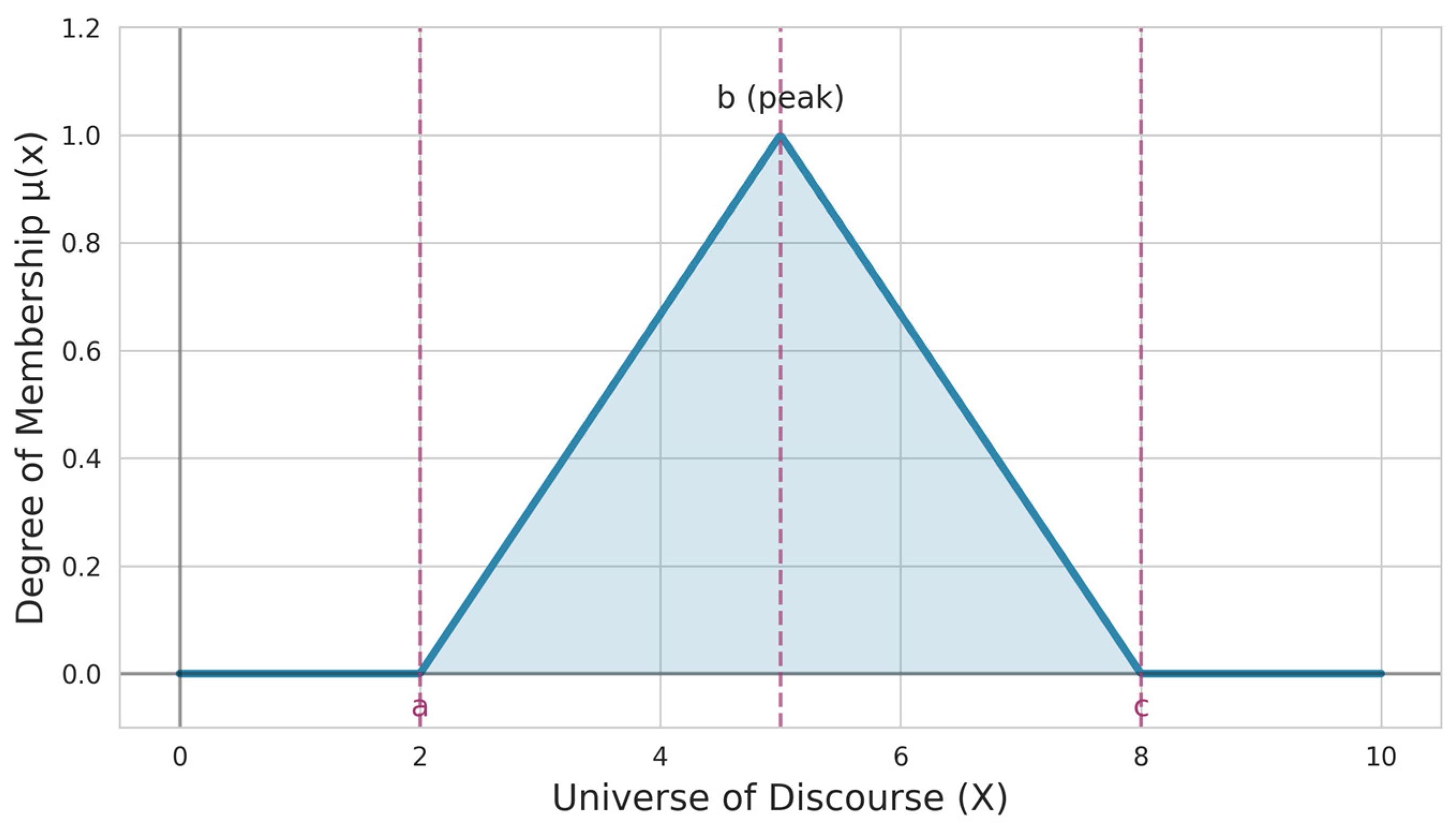
The fuzzy logic apparatus was chosen to realize the road friction coefficient prediction algorithm. A triangular description was selected as a mathematical one for the belonging functions of the output terms. The graphical view of the triangular belonging function is presented in Figure 3.

This fuzzy logic membership function is described by the following formula:

$${\mu }_A\left(x\right)=\left\{ \begin{array}{c}{\displaystyle \frac{x-a}{b-a}}, a\le x\le b\\ {\displaystyle \frac{c-x}{c-b}}, b\le x\le c\\ 0, x<a if x>c\end{array}\right.$$

(5)

The output parameter determined using the fuzzy logic apparatus will be the road friction coefficient φ [16]. The rules were developed to determine the fuzzy logic output parameter φ depending on the input conditions. These parameters are presented in

Table 2. Rules of belonging of the road friction coefficient.

$\mathit{t}, \mathbf{°}\mathbf{C}$	Precipitation Sensor	Precipitation Intensity Sensor	ABS	ESP	LDWS	Timer (min)	φ
<0	+	high	+	+	−	>5	1
<0	+	high	+	+	+	<5	2
<0	+	low	+	+	+	<5	3
<0	+	low	+	−	+	<5	3
<0	−	off	−	−	+	-	5
>0	+	low	+	−	+	<5	4
>0	−	off	+	−	+	<5	4
<0	−	off	−	−	+	-	5
>0	−	off	−	+	+	<5	4
>0	−	off	−	−	+	-	5

.

The degree of object detail depends on the number of terms (partitions into subsets). The decomposition is very important and affects the controller performance in the real control devices [17]. Figure 4a shows a coarse fuzzy decomposition with three terms and three fuzzy subsets. A more detailed decomposition with seven subsets is shown in Figure 4b.

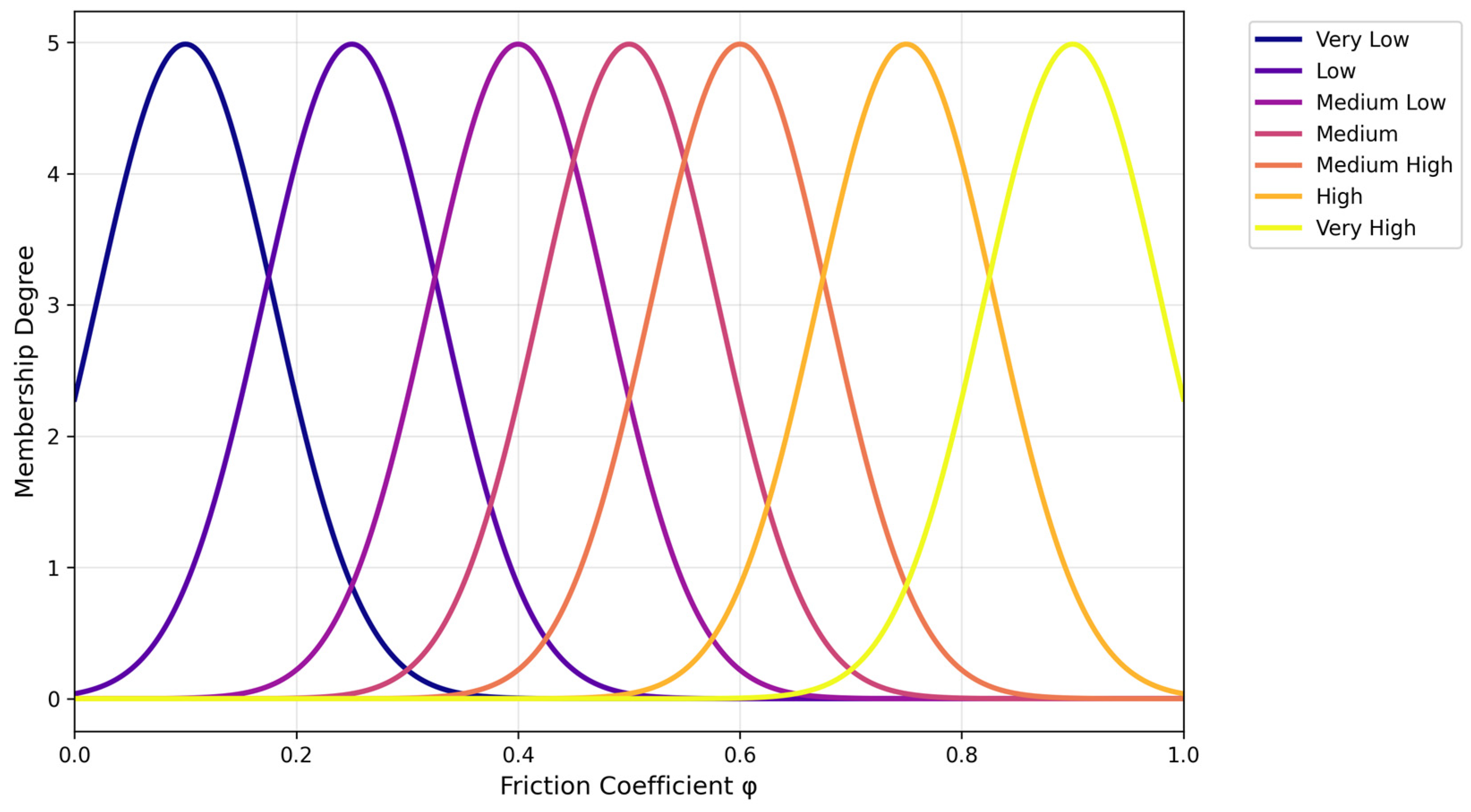
The developed AEB prediction algorithm divides the output terms into seven subsets, which correspond to a certain value of φ [18]. Accordingly, the decomposition is a detailed set of output terms in the range [0…1] and finally has the following form, presented in Figure 5.

Since time appears in the list of input fuzzy logic parameters, we decided to resort to the adaptive fuzzy logic regulator (AFR), since its application in complex control systems with time control shows to be the most effective option. The basics of application for the construction of the fuzzy logic regulator were taken from the textbook by G.L. Demidov and D.V. Lukichev [19].

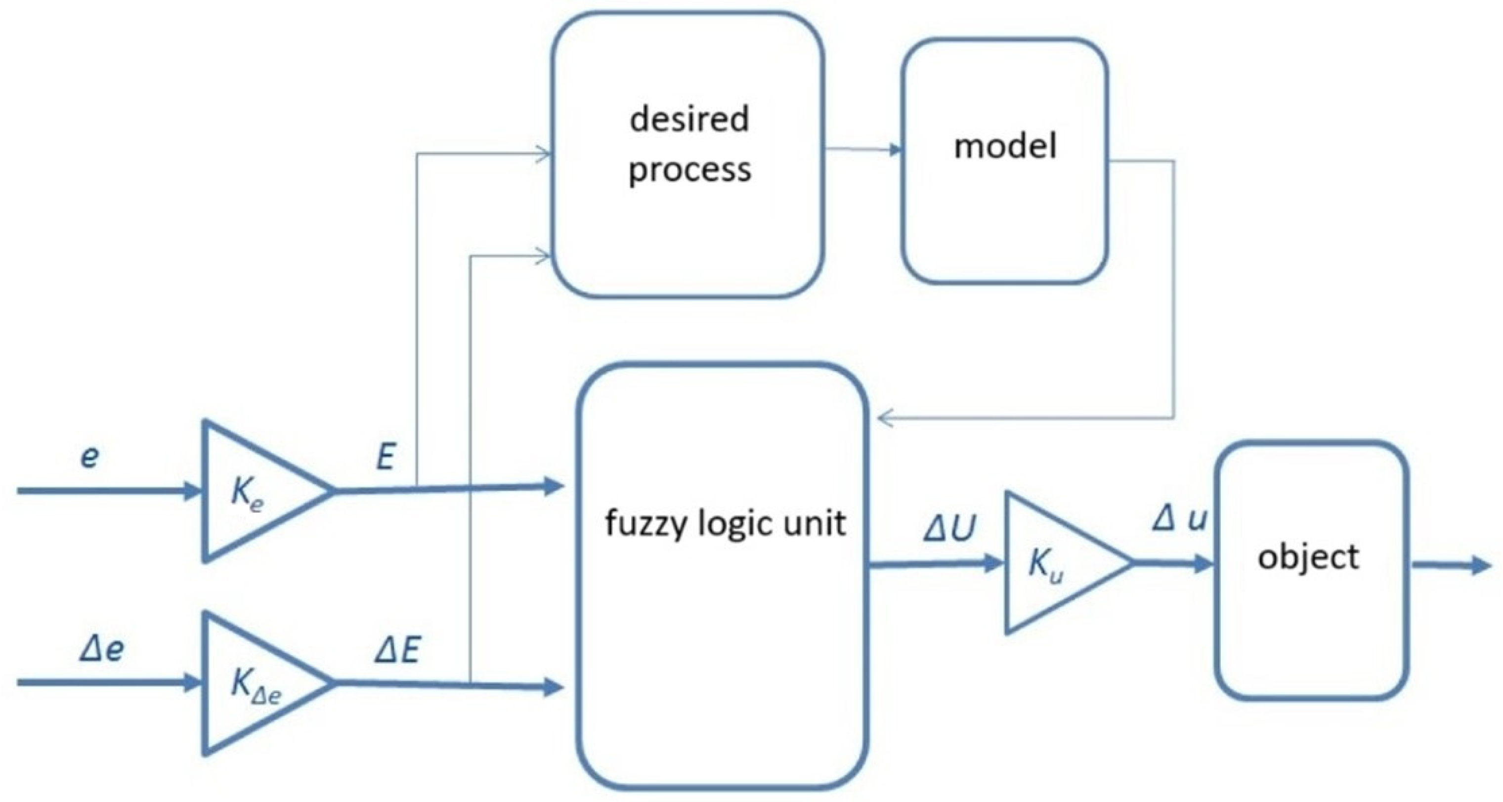
A typical structural diagram of a traditional adaptive regulator is shown in Figure 6. This type of regulator is used in systems with nonlinearly varying disturbances, or when the parameters of the system itself change over time. The adaptive regulator has two loops—an inner control loop, which is the main loop, and the external loop, which is a building block to the main loop [20].

The desired process sets the desired dynamics of the system.

The model represents the rules, providing a linguistic description of the transient process in the system of the same dimensionality as in the BNL.

The fuzzy logic block conducts the procedures of fuzzification, implication, and defuzzification.

To implement the fuzzy logic block (FBL), it was decided to apply Fuzzy toolbox, a MATLAB/Simulink (R2020a) tool. This tool allows the creation of systems with fuzzy logic inference, which can be integrated into the developed mathematical models with subsequent automatic generation into C/C++ code.

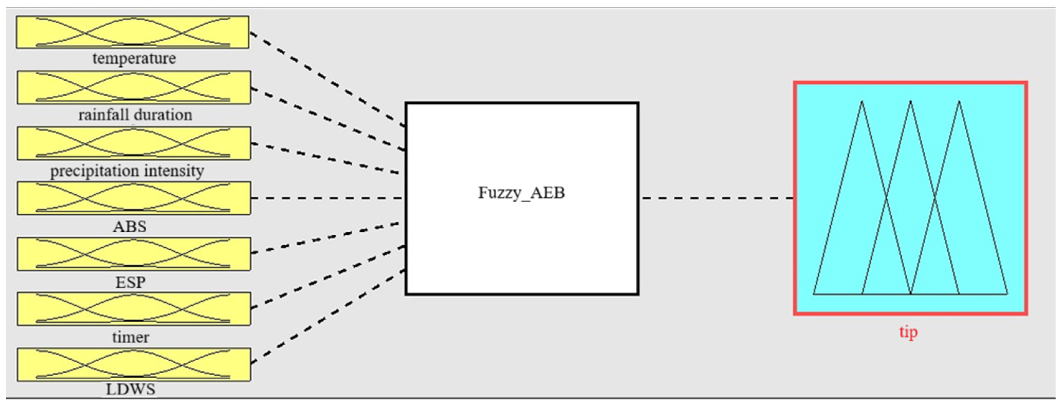
Figure 7 shows the implementation of the developed fuzzy logic algorithm in the MATLAB environment using Fuzzy toolbox [21].

The diagram in Figure 7 shows seven input signals that are used in the Mamdani fuzzy inference system [22]. Each input parameter has its own type of membership function, selected according to the nature of the data (for example, a Gaussian function for temperature, a triangular function for the intensity of the wipers). This implementation allows for modeling and automatic code generation for integration into car control systems.

For each signal, a different kind of input term is given according to the characteristics of the parameter.

Figure 8 shows the type of input parameters according to the ambient air temperature. Here, the Gaussian law of thermal variation is chosen because it allows for flexible adjustment in the near-zero zone of the input parameter [23].

Figure 9 shows the view of the wiper intensity input parameters. In this case, the triangular law of variation in the thermals was chosen because the wiper intensity parameters did not require flexibility in adjustment [23].

The dependence of output terms on input parameters is presented in Figure 10.

Figure 10 shows the dependence of the output road friction coefficient on the input parameters, such as ambient temperature, precipitation intensity, etc. The visualization demonstrates how a change in input variables affects the output value of the road friction coefficient within the framework of the developed fuzzy inference system. The surface reflects the nonlinear nature of the dependence, which confirms the adequacy of using fuzzy logic to model complex and dynamic pavement conditions.

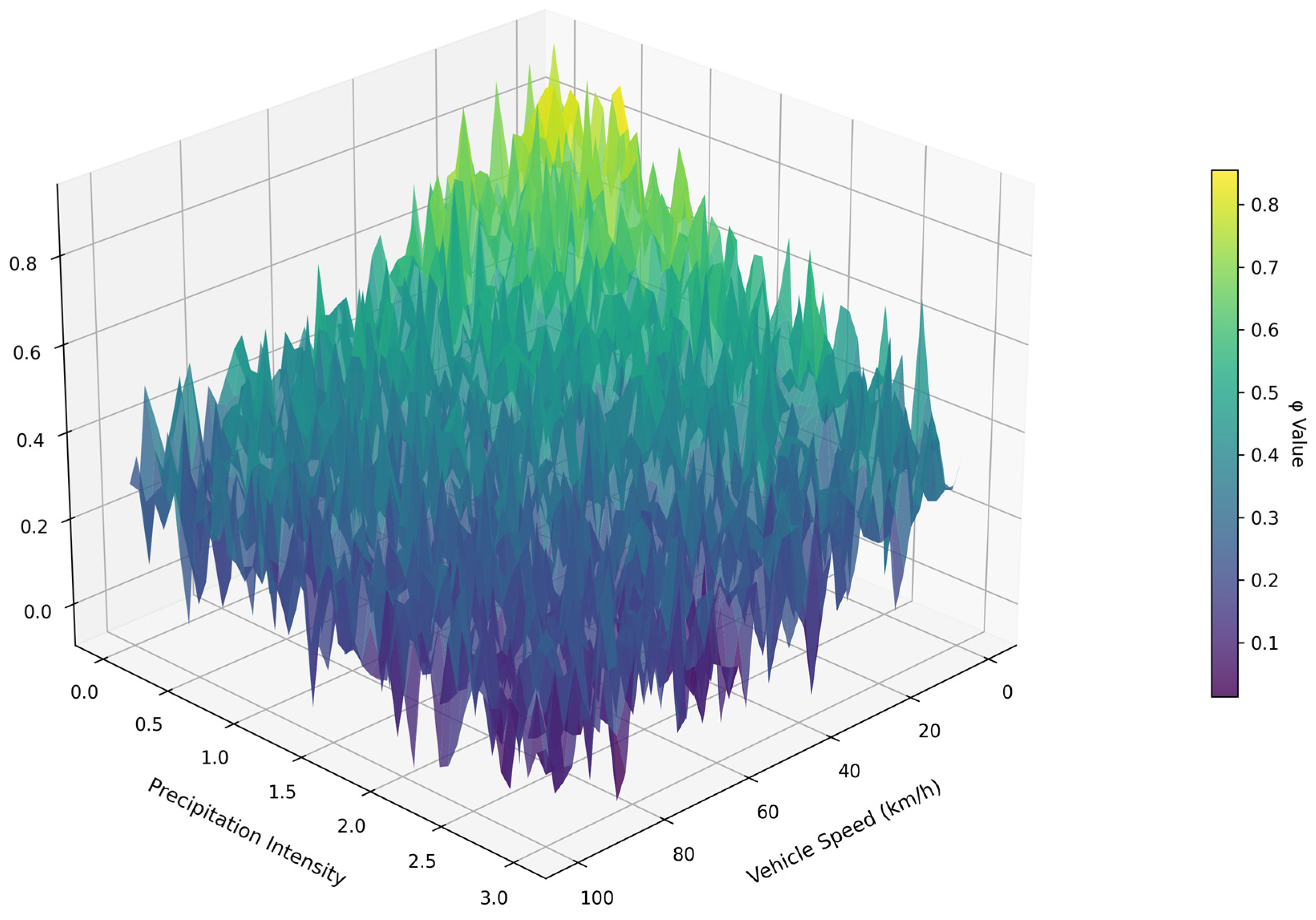
Based on the obtained output parameters modeling the results using the developed fuzzy logic rules, the attribution surface presented in Figure 11 was obtained.

This figure shows the dependence of the road friction coefficient on the TC speed and precipitation. It should be noted that when other parameters to construct the surface are applied, its shape and values change.

3. Test Results and Discussion

The following were selected as indicators characterizing the efficiency of the road friction coefficient prediction algorithm, allowing for an objective comparative evaluation:

$V_{act}$—speed at which the braking was activated;

$j_{st\_d}$—steady-state value of deceleration;

${\phi }_p$—predicted coefficient of grip of the tire with the supporting surface (calculated by means of the forecasting algorithm);

${\phi }_{actual}$—the actual tire grip coefficient.

Since the basic formula for steady-state deceleration is:

$$j_{st\_d}=\phi \times g$$

(6)

$$j_{st\_d}/g={\phi }_{actual }$$

(7)

The proposed parameters should fully reflect the main performance indicators of the system. The main parameter to verify the prediction of the road friction coefficient will be the comparison between the calculated road friction coefficient and the one obtained during the test (${\phi }_{p }$ and ${\phi }_{actual}$).

To verify the calculated road friction coefficient ${\phi }_{p }$, it is necessary to conduct tests, revealing the actual coefficient ${\phi }_{actual }$. In the tests, the obtained data are compared, and the errors of the calculations are analyzed against the actual values.

The comparison of the predicted coefficient of the algorithm and its correlation with the actual experimental value is as follows:

$$∆\phi ={\phi }_p- {\phi }_{actual}$$

(8)

The longitudinal acceleration sensor involved in the ESP system determines the current deceleration values during the tests. The value of the obtained deceleration was the criterion used to evaluate the convergence of the calculated and the experimental data.

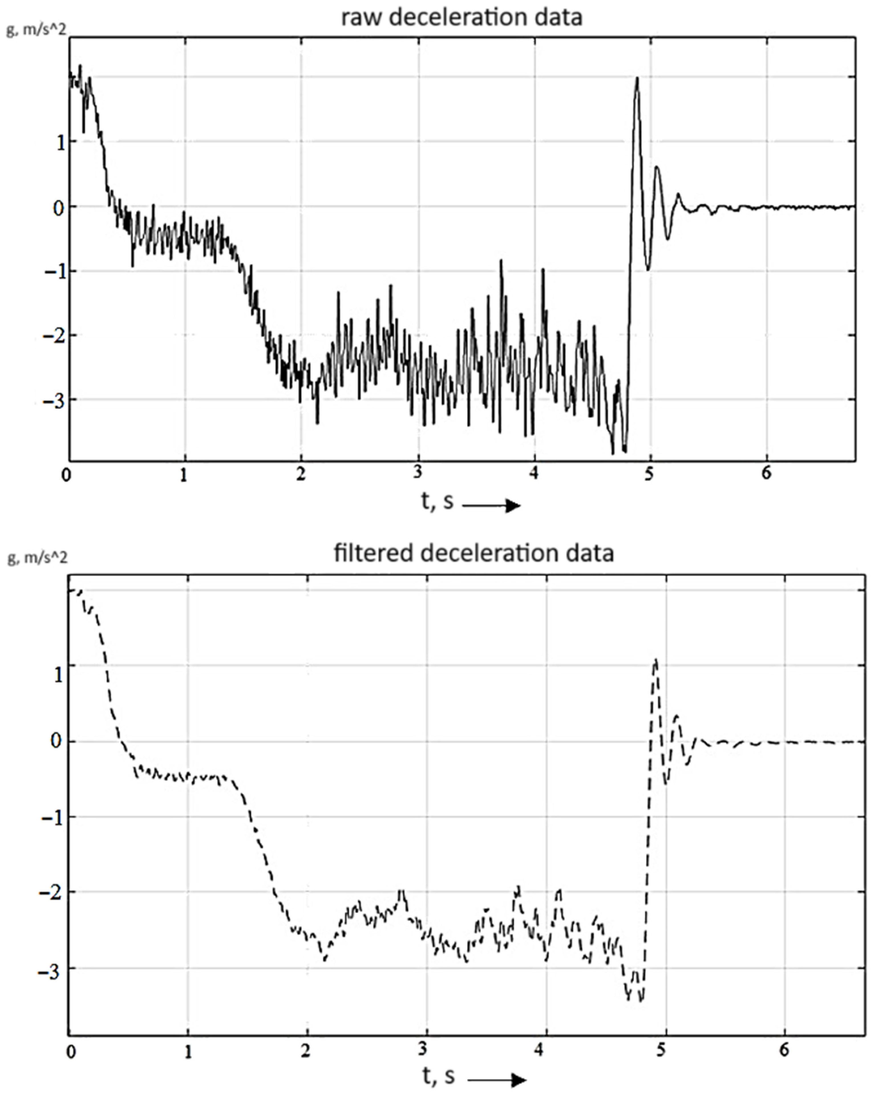
The value of ${\phi }_{actual}$ from the ESP longitudinal acceleration sensor has some scatter and noise. An analysis filter in Simulink was created to analyze the average value of the recorded test log files. Figure 12 shows the schematic of the filter model. The function automatically counts the average steady-state deceleration, which is displayed on the display block.

Figure 13 shows the view of the original signal (upper graph) and the post-filtering one (lower graph).

3.1. Dry Asphalt Tests

The first stage of the experimental study tested the prediction accuracy for the current road friction coefficient when driving on dry asphalt. To determine the road friction coefficient with more accuracy, it is necessary to drive over 5 min in a test vehicle in a test area with the external conditions in which the experimental study is conducted. During this time, the accumulated data allow for the most accurate correction of the coefficients against the current conditions and the correction factors’ value application.

Weather conditions: Ambient temperature 10–15 °C, no precipitation, and mostly sunny.

Road surface: Dry asphalt and no slope.

Speed at the beginning of braking: 20 km/h—100 km/h.

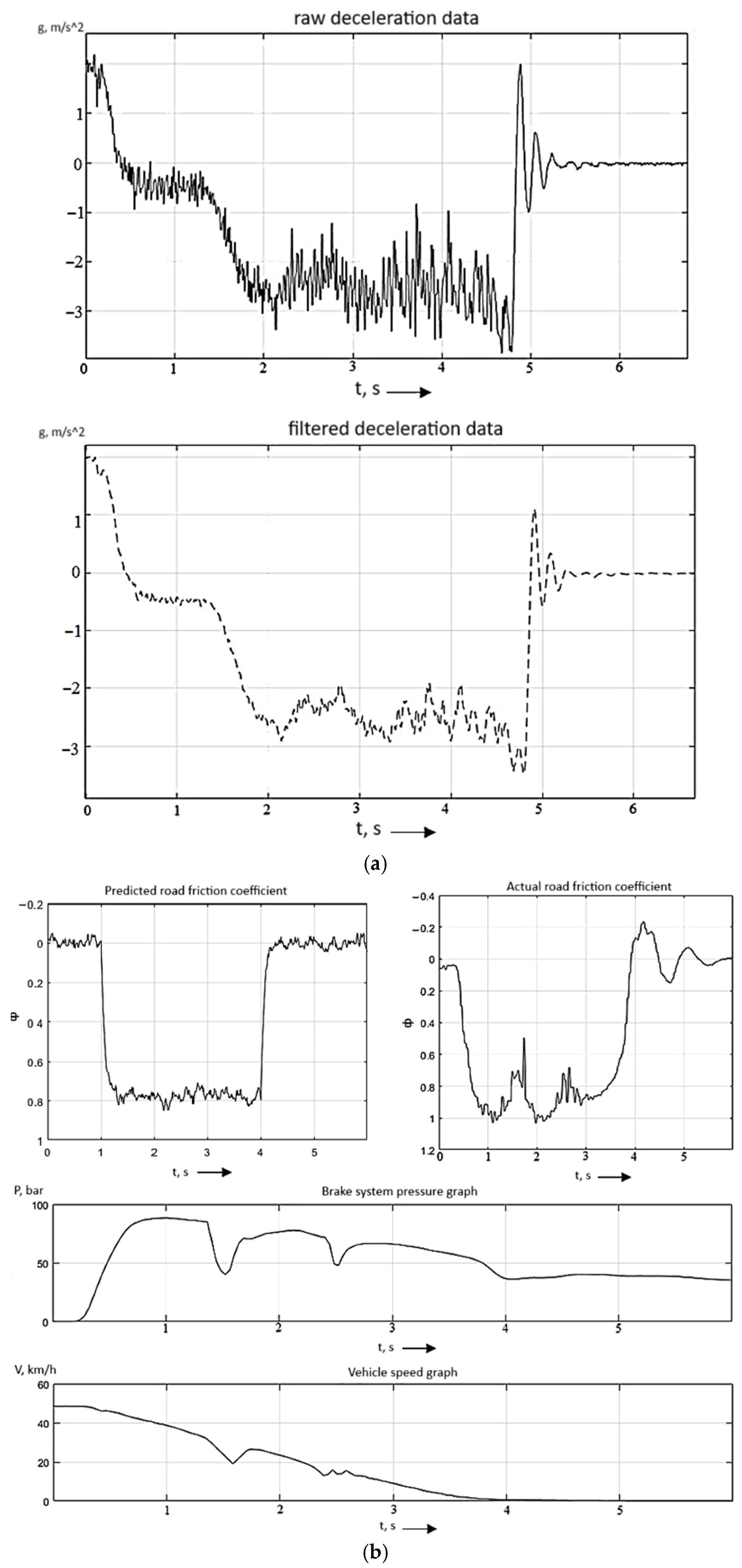
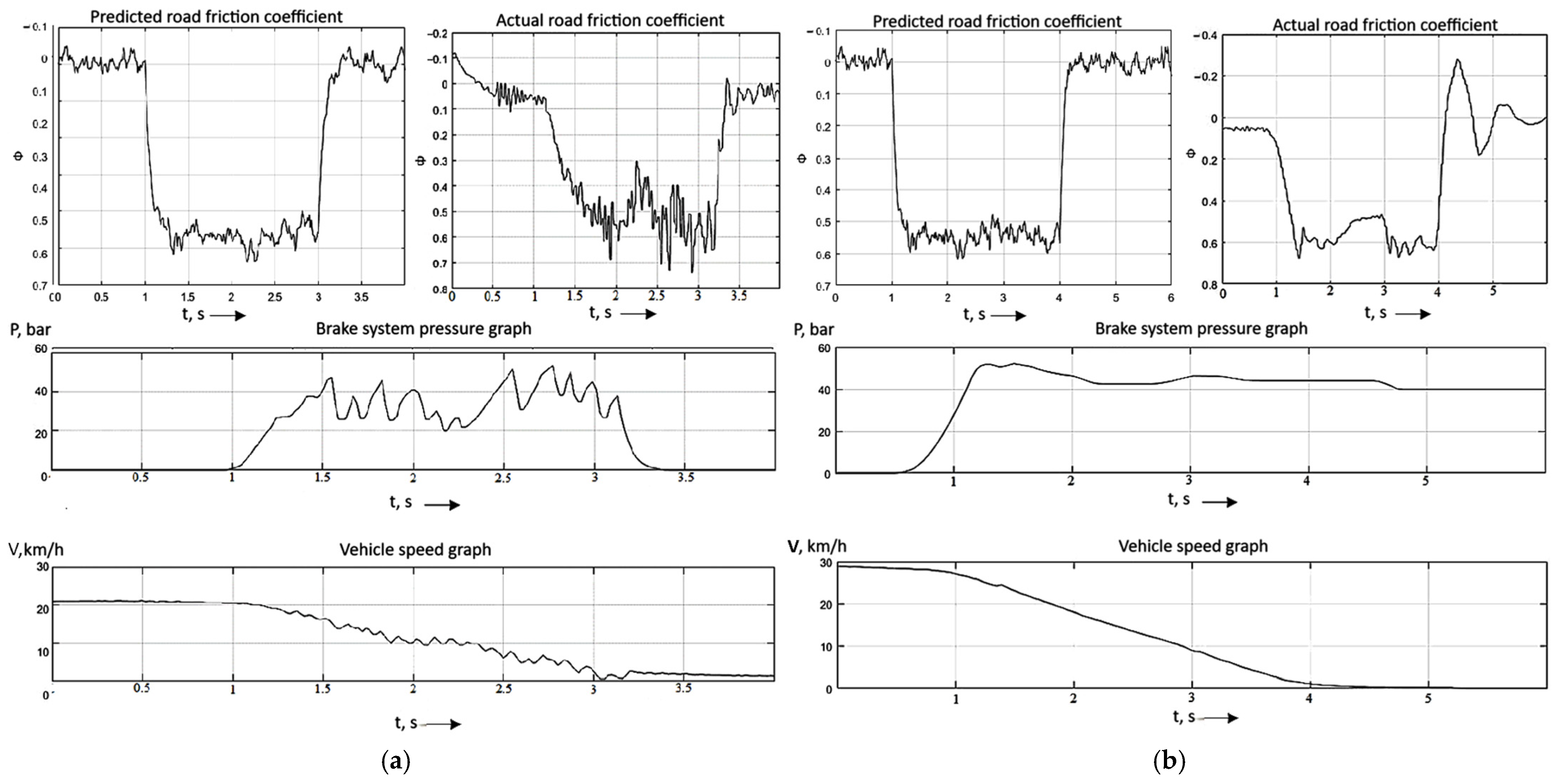
The graphs (Figure 14) show the results of the experimental study of the correlation between the predicted and the actual road friction coefficient. While the vehicle was moving, a braking request from the AEB was applied. The graphs show the predicted road friction coefficient, the actual achieved road friction coefficient, speed, and pressure in the brake system at the time of the experiment.

The dry asphalt test cycle consisted of three runs each at speeds from 20 to 100 km/h—see

Table 3. Results of runs at speeds of 20 to 40 km/h in the dry asphalt tests.

	Race No. 1	Race No. 2	Race No. 3	Race No. 4	Race No. 5	Race No. 6	Race No. 7	Race No. 8	Race No. 9
V (km/h)	20	20	20	30	30	30	40	40	40
${\phi }_{p }$ (predicted value)	0.81	0.81	0.8	0.79	0.78	0.81	0.78	0.79	0.78
${\phi }_{actual }$ (experimental value)	0.78	0.82	0.76	0.81	0.76	0.77	0.78	0.81	0.8
$∆\phi$ (difference in results)	0.03	0.01	0.04	0.02	0.04	0.04	0	0.02	0.02
Error %	3.8	1.2	5.2	2.4	5.3	5.2	0	2.4	2.5

,

Table 4. Results of runs at speeds of 50 to 70 km/h in the dry asphalt tests.

	Race No. 10	Race No. 11	Race No. 12	Race No. 13	Race No. 14	Race No. 15	Race No. 16	Race No. 17	Race No. 18
V (km/h)	50	50	50	60	60	60	70	70	70
${\phi }_{p }$ (predicted value)	0.78	0.77	0.78	0.79	0.82	0.83	0.82	0.81	0.80
${\phi }_{actual }$ (experimental value)	0.79	0.82	0.82	0.82	0.80	0.78	0.79	0.78	0.79
$∆\phi$ (difference in results)	0.01	0.05	0.04	0.03	0.02	0.05	0.03	0.03	0.01
Error %	1.2	6	4.8	3.6	2.5	6.4	3.7	3.8	1.2

and

Table 5. Results of runs at speeds of 80 to 100 km/h in the dry asphalt tests.

	Race No. 19	Race No. 20	Race No. 21	Race No. 22	Race No. 23	Race No. 24	Race No. 25	Race No. 26	Race No. 27
V (km/h)	80	80	80	90	90	90	100	100	100
${\phi }_{p }$ (predicted value)	0.78	0.76	0.75	0.74	076	0.75	0.75	0.75	0.74
${\phi }_{actual }$ (experimental value)	0.77	0.80	0.79	0.78	0.73	0.72	0.72	0.75	0.73
$∆\phi$ (difference in results)	0.01	0.04	0.04	0.04	0.03	0.03	0.03	0	0.02
Error %	1.2	5	5	5	4.1	4.2	4.2	0	2.7

.

According to the results of tests conducted at 20 km/h, the maximum error between the calculated and experimental data is 5.2%; at 30 km/h, the maximum error is 5.3%; and at 40 km/h, the maximum error is 2.5%.

According to the results of tests conducted at a speed of 50 km/h, the maximum error between calculated and experimental data is 6%; at 60 km/h, the maximum error is 6.4%; and at 70 km/h, the maximum error is 3.8%.

According to the results of tests conducted at 80 km/h, the maximum error between calculated and experimental data is 5%; at 90 km/h, the maximum error is 4.2%; and at 100 km/h, the maximum error is 4.2%.

As a result of dry asphalt tests, it was found that the maximum deviations between the calculated and the experimental values did not exceed 6%.

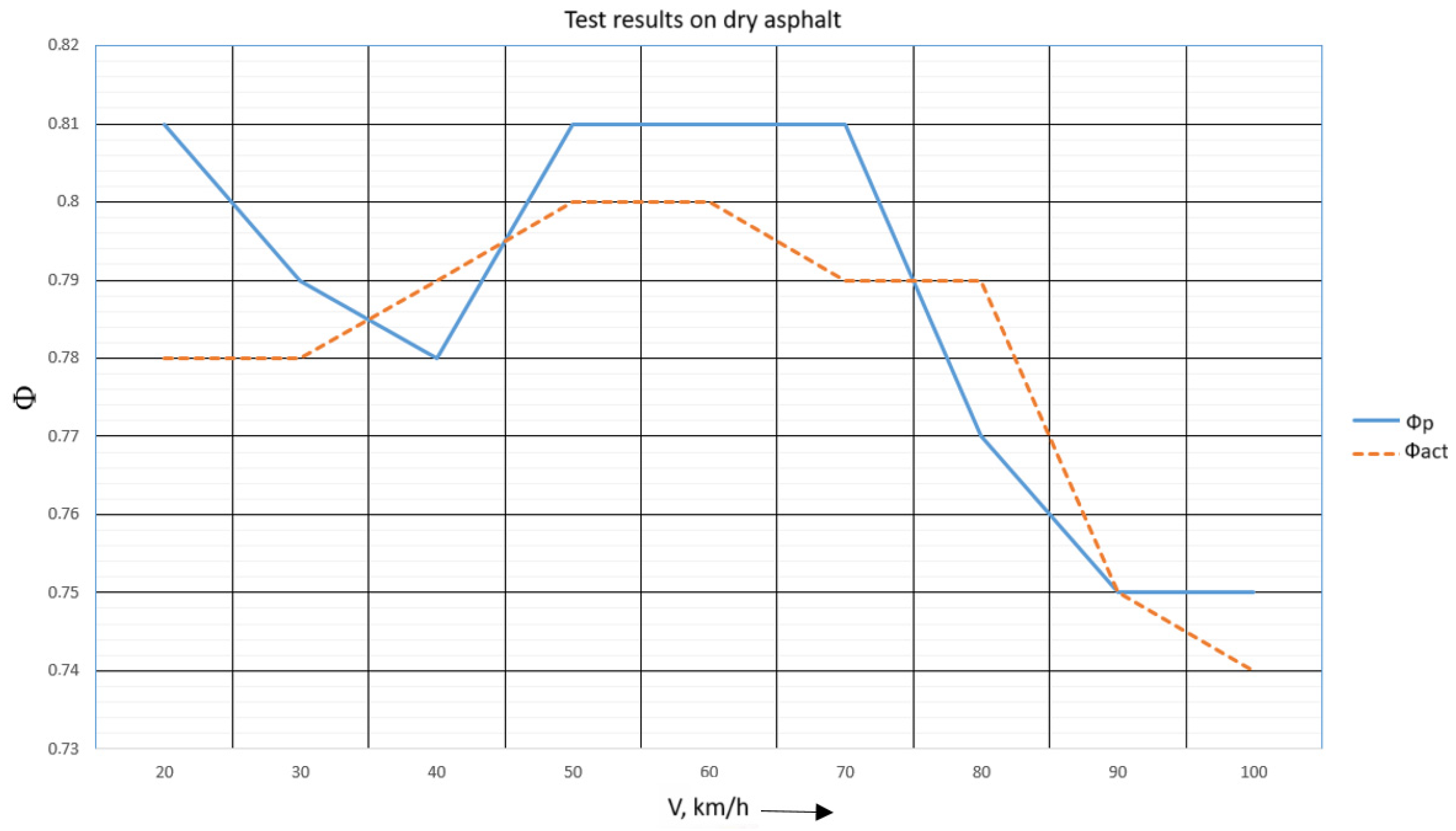
Figure 15 shows the average values of the predicted and actual road friction coefficient on the abscissa axis and the speed of the vehicle on the ordinate axis. The following conclusions can be drawn from the results:

-

On dry asphalt, at speeds up to 70 km/h, the traction properties are constant within the acceptable error range.

-

On dry asphalt, there is a decrease in traction properties at speeds above 70 km/h.

Statistical analysis of the prediction error (Δφ) for all 27 test runs on dry asphalt yields a mean absolute error (MAE) of 0.03 and a standard deviation (SD) of 0.014. The low MAE and SD indicate the high precision and consistency of the prediction algorithm under these conditions.

3.2. Wet Asphalt Tests

Input data:

Weather conditions: Ambient temperature 15–20 °C, precipitation of medium intensity, and overcast.

Road surface: Wet asphalt and no slope.

Speed at the beginning of braking: 20 km/h–100 km/h.

The graphs in Figure 16 show the results of the experimental study of the correlation between the predicted and the actual road friction coefficient. While the vehicle was moving, a braking request from AEB was sent. The graphs show the predicted road friction coefficient, actual achieved road friction coefficient, speed, and brake system pressure at the time of the experiment on wet asphalt.

The following results were obtained from the results of the conducted experiment—see

Table 6. Results of runs at speeds of 20 to 40 km/h in the wet asphalt tests.

	Race No. 1	Race No. 2	Race No. 3	Race No. 4	Race No. 5	Race No. 6	Race No. 7	Race No. 8	Race No. 9
V (km/h)	20	20	20	30	30	30	40	40	40
${\phi }_{p }$ (predicted value)	0.54	0.54	0.55	0.55	0.53	0.53	0.54	0.53	0.51
${\phi }_{actual }$ (experimental value)	0.59	0.56	0.58	0.54	0.54	0.56	0.54	0.54	0.55
$∆\phi$ (difference in results)	0.05	0.02	0.03	0.01	0.01	0.03	0	0.01	0.04
Error %	8.4	3.5	5.1	1.8	1.8	5.3	0	1.8	7.2

,

Table 7. Results of runs at speeds of 50 to 70 km/h in the wet asphalt tests.

	Race No. 10	Race No. 11	Race No. 12	Race No. 13	Race No. 14	Race No. 15	Race No. 16	Race No. 17	Race No. 18
V (km/h)	50	50	50	60	60	60	70	70	70
${\phi }_{p }$ (predicted value)	0.51	0.52	0.50	0.50	0.52	0.51	0.49	0.50	0.48
${\phi }_{actual }$ (experimental value)	0.52	0.49	0.49	0.50	0.50	0.49	0.48	0.48	0.47
$∆\phi$ (difference in results)	0.01	0.03	0.01	0	0.02	0.02	0.01	0.02	0.01
Error %	1.9	6.1	2	0	4	4	2	4	2

and

Table 8. Results of runs at speeds of 80 to 100 km/h in the wet asphalt tests.

	Race No. 19	Race No. 20	Race No. 21	Race No. 22	Race No. 23	Race No. 24	Race No. 25	Race No. 26	Race No. 27
V (km/h)	80	80	80	90	90	90	100	100	100
${\phi }_{p }$ (predicted value)	0.48	0.47	0.46	0.45	0.44	0.44	0.46	0.45	0.42
${\phi }_{actual }$ (experimental value)	0.45	0.45	0.47	0.43	0.45	0.46	0.44	0.44	0.45
$∆\phi$ (difference in results)	0.03	0.02	0.01	0.02	0.01	0.02	0.02	0.01	0.03
Error %	6.6	4.4	2.1	4.6	2.2	4.3	4.5	2.2	6.6

.

According to the results of tests conducted at 20 km/h, the maximum error between calculated and experimental data is 8.4%; at 30 km/h, the maximum error is 5.3%; and at 40 km/h, the maximum error is 7.2%.

According to the results of tests conducted at 50 km/h, the maximum error between the calculated and experimental data is 6.1%; at 60 km/h and 70 km/h, the maximum error is 4%.

According to the results of tests conducted at 90 km/h, the maximum error between the calculated and experimental data is 4.6%; at 80 km/h and 100 km/h, the maximum error is 6.6%.

The error in the experimental and calculated data during all tests on wet asphalt remained at or below 7% for the vast majority of test runs (26 out of 27). A single outlier value of 8.4% was observed at 20 km/h (Race No. 1, Table 6), which can be attributed to the high sensitivity of the prediction algorithm and sensor readings to the initial formation of a water film on the asphalt surface immediately after the onset of precipitation.

Statistical analysis of the prediction error (Δφ) for all 27 test runs on wet asphalt yields a mean absolute error (MAE) of 0.05 and a standard deviation (SD) of 0.012. The larger spread in error compared to dry asphalt reflects the increased variability of wet surface conditions, yet the MAE remains low.

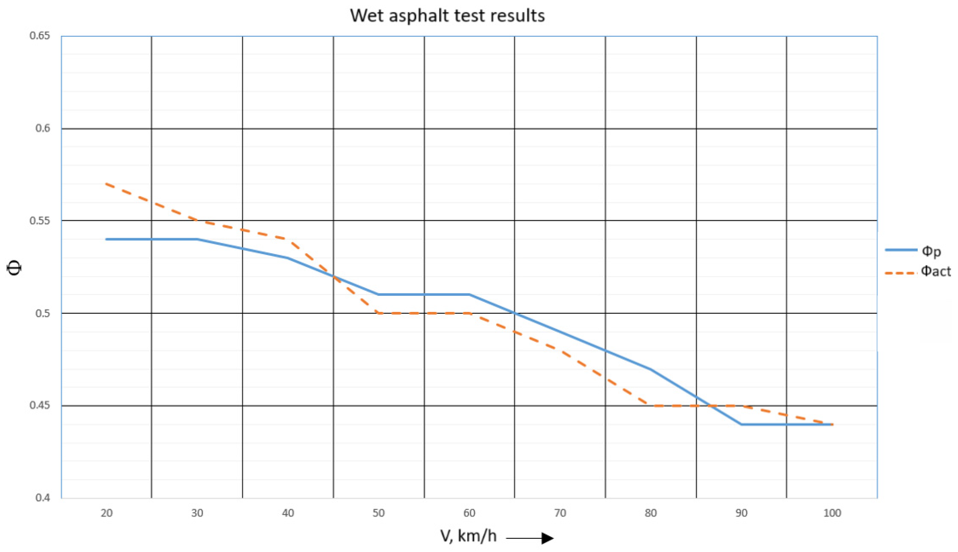
Figure 17 shows the average values of the predicted coefficient of friction and the actual coefficient of friction. The following conclusions can be drawn from the results obtained: on wet asphalt, a decrease in traction properties is clearly observed with increasing speed across the entire speed range.

3.3. Packed Snow Simulation (Wet Basalt Tests)

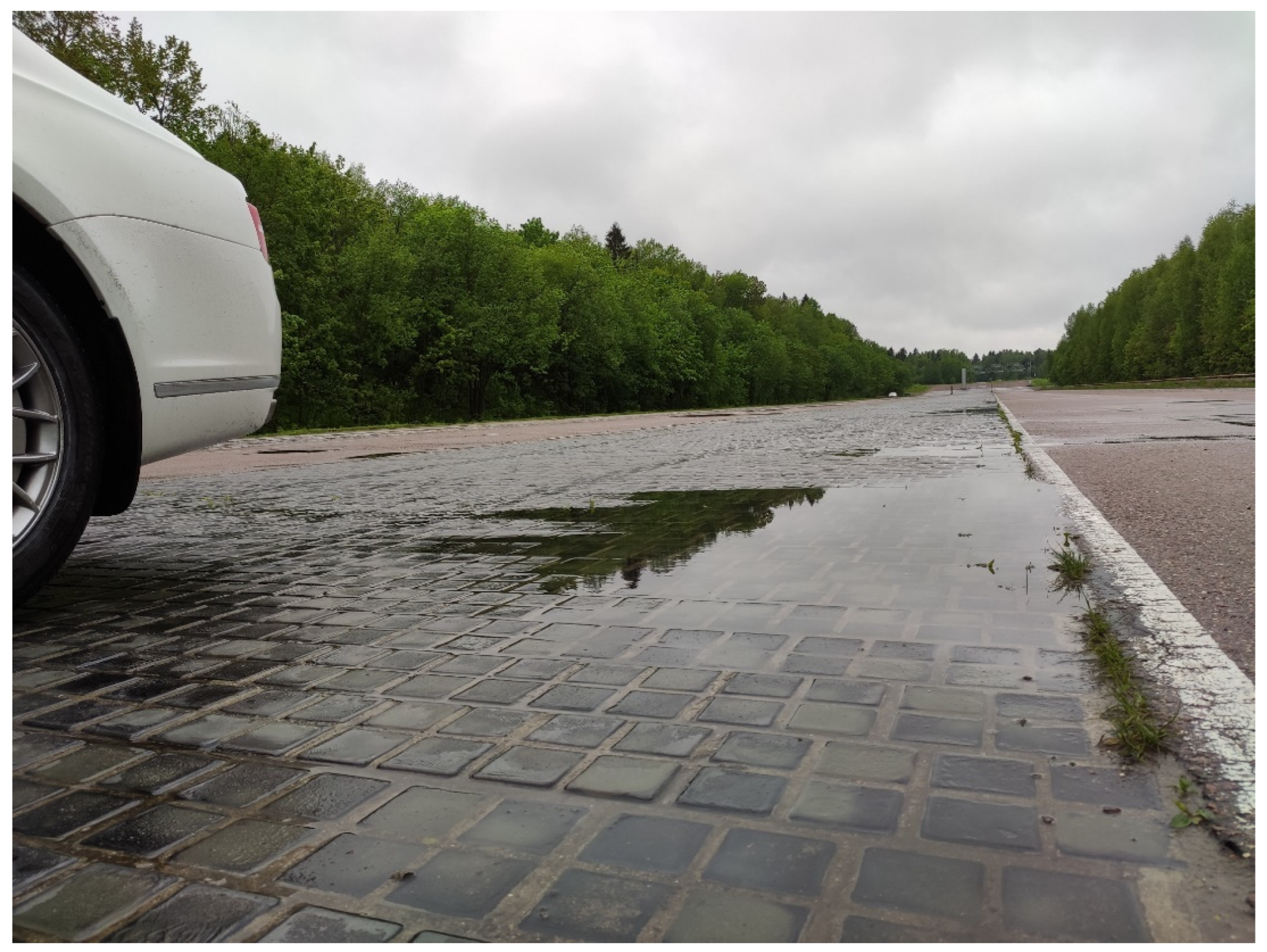
Since wet basalt pavement corresponds to packed snow in terms of friction coefficient, it was used as a reference surface for conducting tests corresponding to packed snow.

The input parameters of the sensors for predicting the coefficient of friction in this experiment were modeled in accordance with the characteristics of movement on compacted snow cover. The data was taken in accordance with the recorded sensor values during winter vehicle testing.

Figure 18 shows a view of the basalt coating on the test site, used to simulate movement on rolled snow. This type of coating was chosen due to the close values of the coefficient of friction to the rolled snow, which made it possible to conduct controlled and repeatable tests in safe conditions. The coating was uniform and without bias, which met the requirements of the experiment.

Input data:

Weather conditions: Ambient air temperature—5 °C, heavy precipitation, and ABS activation in the current movement cycle.

Road surface: Wet basalt and no slope.

Speed: 20 km/h–70 km/h.

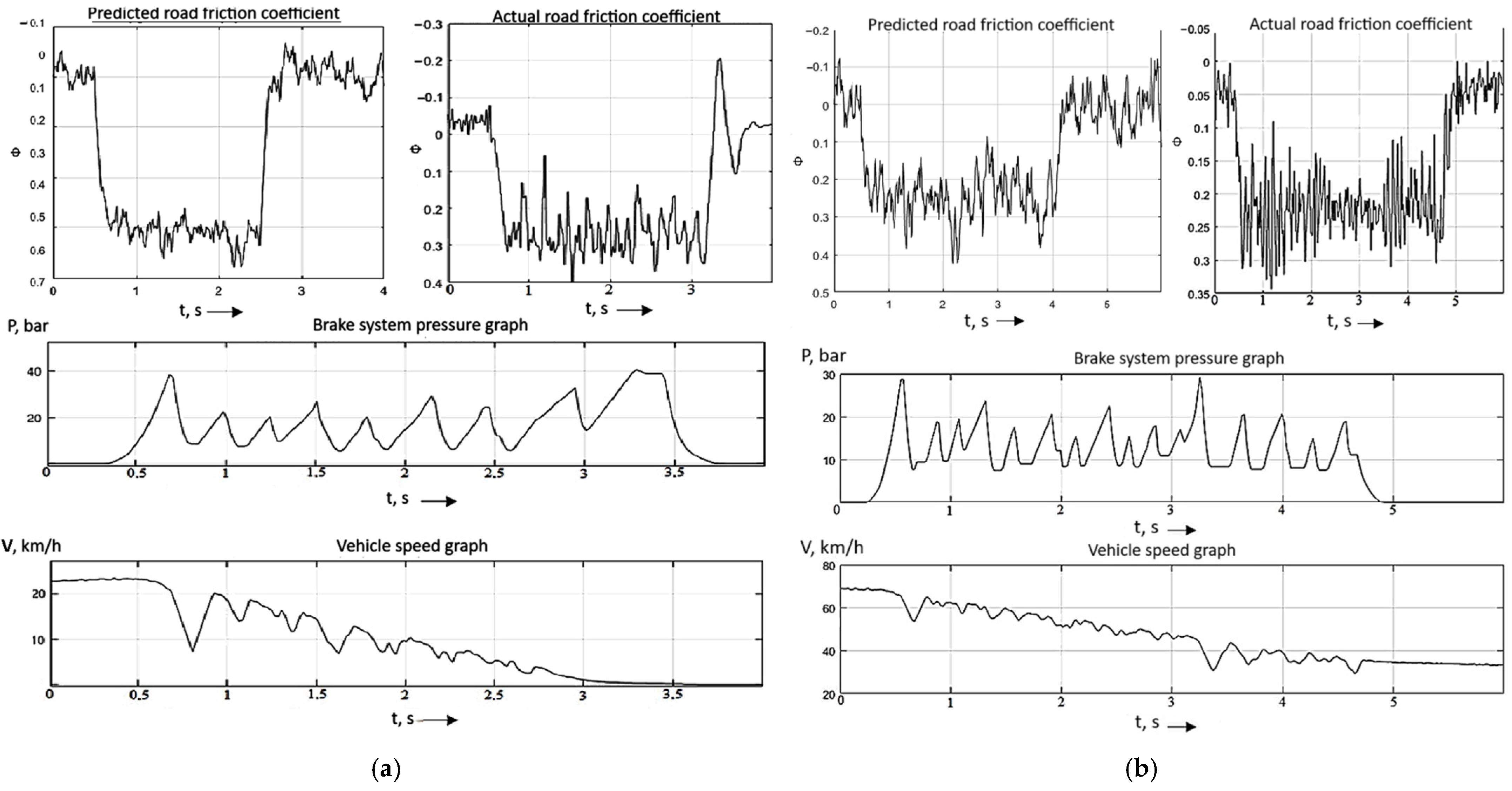
The graphs (Figure 19) show the results of an experimental study of the correlation between the predicted and the actual coefficients of friction on compacted snow. An AEB request was issued while the vehicle was in motion. The graphs show the predicted coefficient of friction, the actual coefficient of friction achieved, the speed, and the pressure in the braking system at the time of the experiment.

According to the results of tests conducted at a speed of 20 km/h, the maximum error between the calculated and experimental data is 10%; at speeds of 30 km/h and 40 km/h, the maximum error is 6.6% (

Table 9. Results of runs at speeds of 20 to 40 km/h on wet basalt tests.

	Race No. 1	Race No. 2	Race No. 3	Race No. 4	Race No. 5	Race No. 6	Race No. 7	Race No. 8	Race No. 9
V (km/h)	20	20	20	30	30	30	40	40	40
${\phi }_{p }$ (predicted value)	0.34	0.33	0.34	0.31	0.33	0.32	0.32	0.31	0.32
${\phi }_{actual }$ (experimental value)	0.32	0.30	0.31	0.30	0.31	0.30	0.30	0.33	0.31
$∆\phi$ (difference in results)	0.02	0.03	0.03	0.01	0.02	0.02	0.02	0.02	0.01
Error %	6.2	10	9.6	3.3	6.4	6.6	6.6	6	3.2

).

According to the results of tests conducted at 50 km/h, the maximum error between calculated and experimental data is 7.4%; at 60 km/h, the maximum error is 7.6%; and at 70 km/h, the maximum error is 8.3% (

Table 10. Results of runs at speeds of 50 to 70 km/h on wet basalt tests.

	Race No. 10	Race No. 11	Race No. 12	Race No. 13	Race No. 14	Race No. 15	Race No. 16	Race No. 17	Race No. 18
V (km/h)	50	50	50	60	60	60	70	70	70
${\phi }_{p }$ (predicted value)	0.29	0.30	0.29	0.28	0.27	0.28	0.26	0.26	0.27
${\phi }_{actual }$ (experimental value)	0.27	0.28	0.28	0.27	0.27	0.26	0.24	0.25	0.25
$∆\phi$ (difference in results)	0.02	0.02	0.01	0.01	0	0.02	0.02	0.01	0.02
Error %	7.4	7.1	3.5	3.7	0	7.6	8.3	4	8

).

Statistical analysis of the prediction error (Δφ) for all 18 test runs on wet basalt yields a mean absolute error (MAE) of 0.02 and a standard deviation (SD) of 0.08. The highest SD here aligns with the challenging and variable nature of low-friction surfaces, but the MAE confirms the model’s overall accuracy remains high.

Figure 20 shows the average values of predicted road friction coefficients and actual road friction coefficients. The following conclusions can be drawn from the results: on rolled snow, there is a clear decrease in traction properties under braking with increasing speed.

The comparison of the results of the computational and experimental studies indicates a close convergence. The maximum discrepancy between the predicted and actual road friction coefficient is under 10%. The character of the change in the calculated values corresponds to the experimental ones. This indicates a significant degree of adequacy of the developed mathematical model.

4. Conclusions

The development of accurate and robust friction estimation methods remains a key challenge for the deployment of reliable ADASs [24]. This study has presented a fuzzy-logic-based methodology that demonstrates high predictive accuracy (<10% error) across dry asphalt, wet asphalt, and wet basalt surfaces, the latter simulating the friction properties of packed snow.

A limitation of this study is the validation in simulated winter conditions (wet basalt) rather than natural ice and snow. This approach was chosen to ensure experimental repeatability and safety. However, the results on wet basalt provide a strong proof-of-concept for the model’s performance in low-friction scenarios.

Future work will focus on expanding the validation scope to include real-world winter conditions. Planned activities include controlled testing on ice, fresh snow, and packed snow at a winter proving ground. Furthermore, we plan to enhance the sensor fusion algorithm by incorporating infrared road surface temperature data and optical infrared camera inputs to improve the detection of black ice and other transparent ice layers, which represent particularly challenging and critical scenarios for ADAS performance.

The applicability of the mathematical model is confirmed by a modeling error of less than 10% across the tested scenarios, which is an acceptable value given the specifics of how the system functions and provides a robust foundation for further development and integration into vehicle safety systems. The technique for predicting road friction coefficients is based on fuzzy logic principles. The use of a temperature sensor, a precipitation intensity sensor, and information on the triggering of the car’s anti-lock braking system, directional stability system, and road marking line recognition system are justified for the realization of the fuzzy controller.

The reliability of the road friction coefficient forecast has been confirmed experimentally: tests have been carried out to check whether the actual road friction coefficient corresponds to the predicted value for three types of pavement: dry asphalt, wet asphalt, and rolled snow.

According to the test results, the maximum error values obtained are as follows:

-

6% on dry asphalt;

-

6.6% on wet asphalt;

-

8.3% on wet basalt.

Thus, the satisfactory convergence of the results of the theoretical and experimental studies is achieved. The applicability of the mathematical model is confirmed by a modeling error of less than 10%, which is an acceptable value given the specifics of how the system functions.