3D Models for Structural Analysis—Tests on Procedures and Point Cloud Processing ^†

Abstract

In recent years, Neural Radiance Fields (NeRFs) and 3D Gaussian Splatting (3DGS) have emerged as promising new approaches for 3D reconstruction. NeRFs rely on neural fields that generate a three-dimensional representation of a scene from photographs, estimating reflectance properties and reconstructing the underlying geometry. Since their introduction in 2020, NeRFs have attracted significant attention due to their wide range of potential applications. Conversely, 3D Gaussian Splatting (3DGS), introduced in 2023, employs Gaussian primitives to efficiently model objects and structures, offering a flexible and adaptive representation of 3D scenes. Starting from an established pipeline for the use of reality-based models for structural analysis, this paper investigates the performance of 3DGS in handling complex geometries and surfaces characterised by challenging acquisition conditions.

1. Introduction

Three-dimensional (3D) surveying for cultural heritage documentation and conservation is grounded in well-established methodologies, and the integration of multiple acquisition techniques is now considered standard practice. Among these, photogrammetry represents a passive approach capable of generating textured 3D point clouds. It is generally more cost-effective and versatile than Terrestrial Laser Scanning (TLS). However, unlike TLS, photogrammetry is not inherently metric without appropriate control and calibration procedures, is sensitive to lighting conditions, and requires a certain level of operator expertise. Conversely, TLS provides high metric reliability but may encounter limitations in capturing fine details or small-scale features. In the field of computer graphics, particularly in 3D rendering, Neural Radiance Fields (NeRFs) and 3D Gaussian Splatting (3DGS) have recently emerged as prominent techniques. A comparative analysis of Structure from Motion (SfM), Neural Radiance Fields (NeRFs), and 3D Gaussian Splatting (3DGS) reveals significant methodological and conceptual distinctions in approaches to 3D reconstruction and scene representation.

Structure from Motion (SfM) is a geometry-oriented photogrammetric method that reconstructs sparse or dense three-dimensional point clouds from overlapping two-dimensional images. This is achieved through feature detection and matching, followed by the estimation of intrinsic and extrinsic camera parameters. SfM is extensively employed in cultural heritage documentation due to its methodological robustness, transparency, and compatibility with established surveying practices. Although it can yield highly accurate geometric reconstructions under appropriate acquisition conditions, SfM does not inherently account for view-dependent reflectance effects or complex light transport phenomena.

Neural Radiance Fields (NeRFs) [1] introduce a learning-based framework for volumetric reconstruction. Rather than producing explicit geometric primitives, NeRFs model a scene as a non-stop volumetric task encoded within a neural network. This function records three-dimensional coordinates and inspecting guidelines to colour and density values, thereby implicitly representing geometry within a radiance field. Compared with SfM, NeRFs demonstrate superior performance in photorealistic rendering and in modelling view-dependent visual effects, including specular reflections and complex illumination conditions. However, this approach typically entails substantial computational demands, dense spatial sampling during both training and inference, and careful optimisation. Moreover, the extraction of explicit and metrically reliable geometric information suitable for quantitative or structural analysis remains a challenging process.

3D Gaussian Splatting (3DGS) [2,3] may be regarded as an intermediate solution that integrates aspects of explicit geometric representation with volumetric rendering strategies. In this approach, a scene is represented as a gathering of anisotropic three-dimensional Gaussians, each defined by spatial coordinates, covariance matrices, opacity values, and radiance attributes. Rendering is accomplished through rasterisation-based projection and compositing of these Gaussian primitives. Relative to NeRFs, 3DGS significantly reduces computational requirements and enables real-time rendering, making it particularly suitable for large-scale environments, interactive applications, and rendering diffuse or visually indistinct objects, as well as semi-transparent materials, where the representation of volumetric density or intensity variations within a spatial domain is required [4]. Compared to SfM, it incorporates volumetric radiance modelling, although the geometry remains discretely defined rather than continuously parameterised. Despite its high visual fidelity and computational efficiency, the geometric accuracy of 3DGS and its suitability for metric or structural applications require further systematic assessment.

In conclusion, SfM emphasises explicit and metrically controlled geometric reconstruction; NeRFs prioritise continuous, photorealistic volumetric representation with implicit geometry; and 3D Gaussian Splatting provides a computationally efficient, discrete volumetric approximation optimised for real-time visualisation. The selection of a given methodology should be guided by the specific objectives of the project, whether these concern geometric precision, photorealistic rendering, computational performance, or integration with downstream analytical workflows.

This paper aims to evaluate the performance of 3DGS in the documentation of complex and challenging artefacts, with particular attention to its potential applicability for subsequent structural and mechanical analyses using Finite Element Methods (FEMs), using photogrammetric point clouds as comparison. The procedure that incorporates reality-based models into FEA is well-established and validated [5], so the idea of this work is to analyse if the new trend in 3D data processing can reach the same accuracy of SfM point clouds and hence be processed to be used in FEA. For this purpose, two tools for comparing point clouds in CloudCompare 2.13.2 were used and evaluated: C2C (Cloud-to-Cloud) and M3C2 (Multiscale Model-to-Model Cloud Comparison).

For this purpose, experimental testing was conducted exclusively with 3DGS using the Jawset Postshot V 1.1 platform (https://www.jawset.com).

2. State of the Art

The evaluation of 3D Gaussian Splatting (3DGS) for three-dimensional reconstruction has recently attracted increasing scholarly attention, with applications tested across diverse object types and environmental conditions [6,7,8,9]. Ref. [10] introduced a benchmark framework to assess the quality of Gaussian Splatting outputs, focusing on laboratory datasets and compression performance. In the context of industrial components and controlled environments, Ref. [11] proposed an adaptive reconstruction strategy combined with robust scaling procedures to enhance geometric accuracy relative to ground truth data. The difficulties in the deformation of 3D 3DGS results are analysed and overcome by creating a new method with a mesh-based 3DGS that uses not only the vertex locations but also distortion gradients to guide the 3DGS [12].

Comparative investigations have also been conducted. Ref. [13] performed an analysis of reconstructions generated using Colmap 3.14, NeRF, and 3DGS in outdoor scenarios, evaluating differences in geometric consistency and visual quality [14]. For indoor environments, where accurate spatial data are essential for applications ranging from object detection and virtual reconstruction to Building Information Modelling (BIM), Ref. [15] presented both qualitative and quantitative comparisons of datasets produced using SfM (via Colmap 3.14), NeRF, and 3DGS. In addition, Ref. [16] compared results derived from these methodologies with Simultaneous Localisation and Mapping (SLAM) systems, assessing performance in terms of tracking accuracy, mapping fidelity, and view synthesis capabilities. A free-photogrammetry method was proposed in [17], leveraging both explicit geometric representation and the endurance of the input video stream. 3DGS was also compared to LiDAR for the documentation, preservation, and segmentation of the 3D point cloud of architectural heritage [18] to address the fact that 3DGS works better in the virtual environment for architectural data. In the same direction is [19] that investigates the use of 3DGS for immersive environments while [20] analyses the impact of 3DGS in the creation of virtual museums. All the papers underline the superior visual effects of 3DGS compared to photogrammetry, in the case of virtual tools.

In the context of accurate cultural heritage documentation, many papers presented a modified version of the original method. Ref. [21] presented a modified 3DGS approach optimised for cultural documentation focusing on the improvements of inaccurate image alignment, undesirable background data, and incomplete data due to inadequate photographic coverage. A dual-prior-driven 3DGS structure is presented in [22], in which a feature-aware sampling algorithm builds a detailed geometric prior with absolute scale from the input cloud and then an ideal visual prior provides supervision by generating synthetic views from it. Finally, Ref. [23] proposes an end-to-end framework combining a convolution–Transformer hybrid super-resolution network with an enhanced 3D Gaussian Splatting pipeline. Within the fields of architecture, Ref. [24] examined data representation strategies by comparing NeRF, 3DGS, and SfM-MVS workflows. Ref. [25] investigated the geometric accuracy of 3DGS for orthophoto generation in cultural heritage digitisation, benchmarking results against Terrestrial Laser Scanning (TLS) and Multi-View Stereo (MVS) data. Furthermore, comparative studies have been extended to underwater environments. Ref. [26] evaluated Neural Radiance Fields (including SeaThru-NeRF) and 3D Gaussian Splatting against conventional SfM workflows, highlighting methodological strengths and limitations under challenging imaging conditions. Regarding the reconstruction of fine geometric details, Ref. [8] proposed a homodirectional view-space positional gradient-based densification method that improves detail recovery through Gaussian splitting strategies. Other studies, such as [27], have explored optimisation techniques for 3DGS by constraining the number of Gaussians, thereby achieving improved rendering efficiency while maintaining or enhancing visual quality. No contributions seem to investigate the direct use of 3DGS results for Finite Element Analysis (FEA) purposes. Overall, the current body of literature demonstrates a growing interest in assessing the geometric reliability, rendering performance, and application-specific suitability of 3D Gaussian Splatting across a broad spectrum of domains.

3. Materials and Methods

3.1. SfM Processing

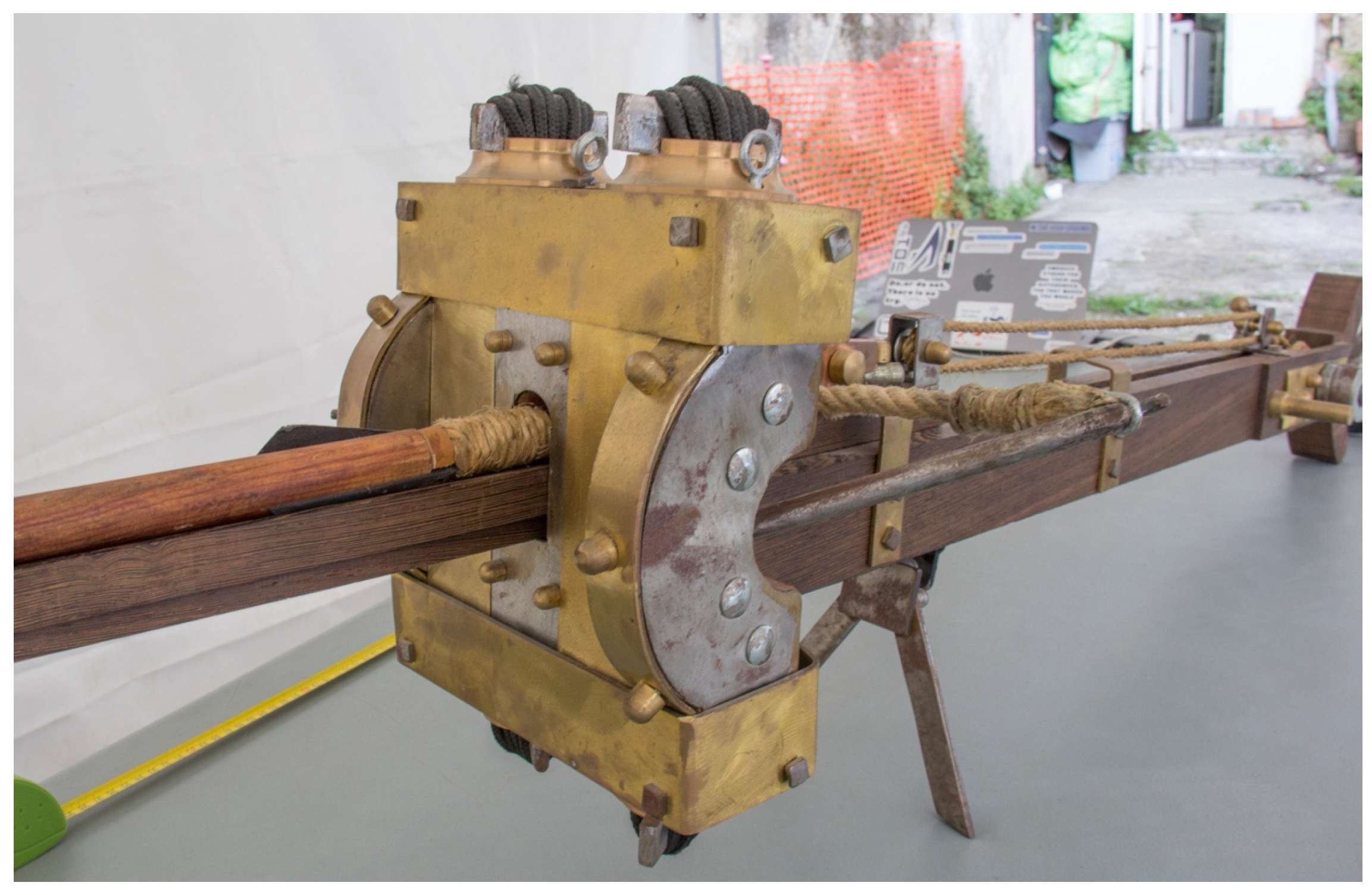
The object used for the tests is a reproduction of a Xanten-Wardt I sec AD Scorpionide (a war throwing machine used in the Roman period for sieges), recreated by Flavio Russo for Archeotecnica.com, 89122 Reggio Calabria, Italy in a scale of 1:1 [28]. The real object was found in 1999 on the bottom of what is known today as Lake Sudsee in the government district of Düsseldorf. This object was chosen because of its intricate and detailed geometry and minute and fine parts (Figure 1).

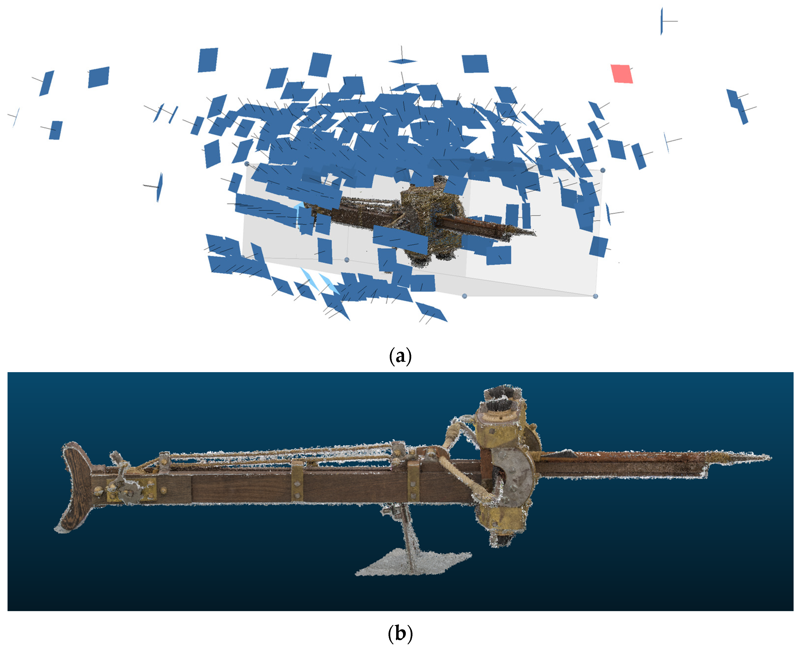
The survey was performed using a Canon 60D APS-C camera (Canon Inc., Tokyo, Japan) coupled with a 60mm macro lens that helped acquire the small details, with the following settings: ISO 500, f/9. The point cloud obtained with Agisoft Metashape 2.2.1, which counted 3,693,711 points (Figure 2), was scaled using specific targets with a Ground Sample Distance (GSD—distance between pixel centres, indicating the smallest detail visible in an image) equal to 0.71 mm, calculated using the equation that considers the pixel size of the camera following the theory for close-range photogrammetry, expressed in millimetres:

$${\displaystyle \frac{\mathrm{p}\mathrm{i}\mathrm{x}\mathrm{e}\mathrm{l} \mathrm{s}\mathrm{i}\mathrm{z}\mathrm{e}\times \mathrm{d}\mathrm{i}\mathrm{s}\mathrm{t}\mathrm{a}\mathrm{n}\mathrm{c}\mathrm{e}}{\mathrm{f}\mathrm{o}\mathrm{c}\mathrm{a}\mathrm{l} \mathrm{l}\mathrm{e}\mathrm{n}\mathrm{g}\mathrm{t}\mathrm{h}} \mathrm{hence} {\displaystyle \frac{0.043\times 1000}{60}} = 0.71}$$

(1)

The point cloud was cleaned using a denoising algorithm that allowed us to remove all the noisy points to generate a point cloud more coherent with the original object surveyed, and then it was compared in CloudCompare 2.13.1 with the original one to assess its accuracy, yielding a mean of 0.0002883 m and a standard deviation of 0.000284 m [29].

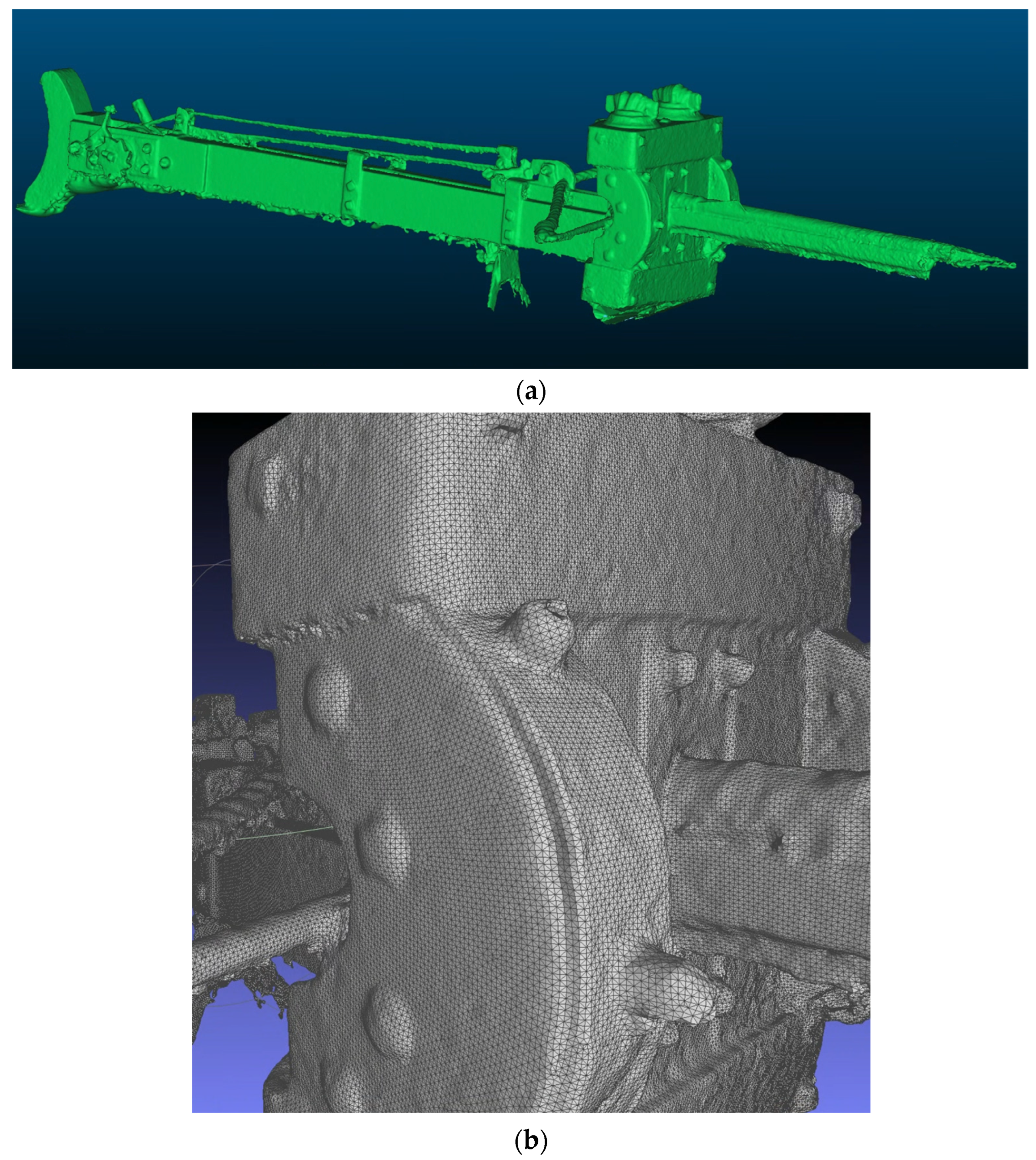
This cleaned point cloud was then transformed into a mesh using Agisoft Metashape 2.2.1 again and then simplified with retopology procedures with the InstantMeshes free repository, obtaining a final model of 1,336,682 quadrangular elements (Figure 3a,b).

This simplified mesh is more suitable to be transformed into a volume for the direct use of the model in FEA software. The accuracy of the initial mesh can strongly influence the final result. This is why it is mandatory to clean the point cloud by excluding all the unnecessary points that can cause wrong measurements, low accuracy, and hence more uncertainty in the final FEA calculation. The retopology process, even when adding a sort of smoothing to the surface of the mesh while strongly decreasing the number of polygons, has been certified to maintain a good closeness to the initial model [5]. The creation of a volumetric model is necessary for performing structural analysis since the objects analysed cannot be discretised into simple shapes such as bars or planes.

3.2. 3DGS

The point cloud was created with Agisoft Metashape 2.2.1 to provide a ground truth, and then with Colmap 3.14, using the typical pipeline:

• Feature detection/extraction;
• Feature matching and geometric verification;
• Sparse reconstruction;
• Bundle adjustment refinement;
• Dense reconstruction.

This passage was necessary since the PostShot platform can automatically read the extrinsic and intrinsic parameters exported from Colmap 3.14 and can use them to process the training of the algorithm. PostShot is, in fact, a tool to perform NeRF and 3DGS in an intuitive way and can compute camera poses. Since the purpose of this paper is to compare the results of the different settings of this tool with a photogrammetric result, we decided to use the same internal and external parameters as the starting point for the subsequent process. Furthermore, using existing alignment typically enhances the quality of the created splats and allows us to generate metrically scaled scenes without much computational effort. Hence, the *.ply of the dense point cloud and the camera parameters computed in Colmap 3.14 were exported and used on the PostShot platform to test the 3DGS outcomes. In this way, all the resulting data had the same internal and external orientation. For the tests, all three radiance field representations available in PostShot were used, exported, and compared to the Metashape 2.2.1 point cloud. The process required choosing different settings after importing the images and performing camera alignment and calibration.

The descriptions were taken from the official website of the tool (https://www.jawset.com/):

• The radiance field profile consists of the reconstruction part.

  i.  

  The best option is supposed to be Splat3, which can best reconstruct fine details in both the foreground and background. Compared to the other profiles, it can also better utilise the details of higher-resolution images.

  ii.  

  Splat3 MCMC uses a more randomised sampling of the scene than the other models. As a result, it may not produce as many fine details.

  iii.

  Splat3 ADC densifies the scene during training. Unlike the Splat3 and Splat MCMC profiles, the Splat ADC profile does not allow specifying the maximum number of splats created. Instead, the Splat Density parameter controls the growth rate of the model size.

• Max Splat Count: This parameter is only available when the Splat3 or Splat MCMC profile is selected. It sets a limit on the total number of Gaussian Splatting primitives that the training process will generate.
• Anti-Aliasing: Checking this option improves the model quality and prevents artefacts when zooming away from the original camera positions.

4. Results

All the data resulting from the different techniques have been compared to understand the level of detail obtained. The main comparison was done with CloudCompare 2.13.2, using both C2C and M3C2 tools.

In this software, the standard deviation (σ) of a Cloud-to-Cloud (C2C) distance calculation represents the spread of measured distances between the compared point cloud and the reference point cloud using a “nearest neighbour search (NNS).” It quantifies how much the individual point-to-point distances deviate from the mean distance value. This method means point movements are always measured relative to the reference point cloud, without differentiating between material uplift and downlift.

M3C2 (Multiscale Model-to-Model Cloud Comparison) calculates the standard deviation (σ) to quantify local surface roughness. This value reflects the variability of points within the core point projection cylinder for each epoch. A key feature of M3C2 is its incorporation of an accuracy estimation approach. The algorithm generates a confidence interval for the distance calculation between point clouds, using individual points as the basis for the assessment. The local roughness values (σ) are then used to estimate distance uncertainty and calculate the Level of Detection (LoD), which helps distinguish true surface change from measurement noise. A plane is estimated from points within a defined radius around the core point, and the standard deviation is computed, providing insights into the surface condition of the surrounding area. Finally, the core point is projected along the normal vector into both point clouds, and the distance between corresponding points—the point cloud difference—is calculated and visualised [30].

The parameter configuration adopted for the comparison was as follows:

• **Core point selection:** entire point cloud.
• **Normal scale:** automatically determined by the software.
• **Projection scale:** automatically determined by the software.
• **Maximum depth:** automatically determined by the software.

Surface normals were derived from the point cloud generated in Metashape 2.2.1.

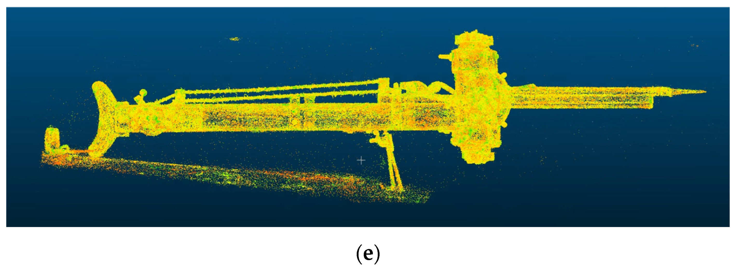
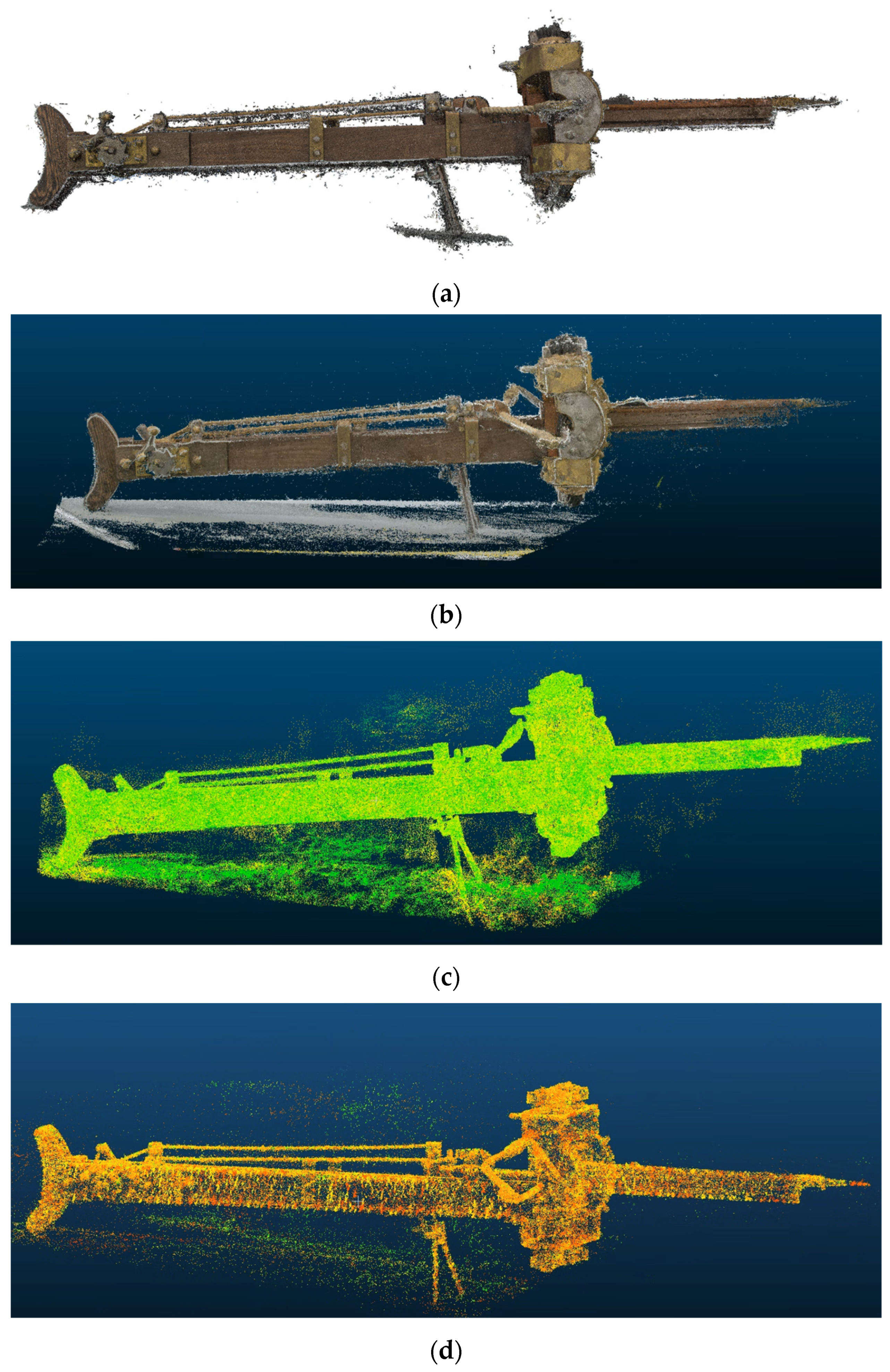
The first comparison was essentially visual, analysing the number of points and the density (

Table 1. Comparison of the number of points in each point cloud obtained with different software.

Software	Number of Points
Agisoft Metashape	3,693,711
Colmap	2,970,255
3DGS SPLAT3	987,178
3DGS SPLAT ADC	286,013
3DGS SPLAT MCMC	1,466,915

; Figure 4a–e).

As expected, Metashape 2.2.1 and Colmap 3.14 gave denser results, while 3DGS gave sparser data, especially with ADC settings. This is probably due to the specifics of the parameter that cannot control the number of splats, and it probably does not handle fine details or complex geometry well. The other two settings gave better results, with MCMC settings providing denser data. It is interesting to note that from the tutorial of the PostShot platform, the best setting should be SPLAT3, which can theoretically reconstruct better fine details, while MCMC should be more random and hence not suitable for tiny parts.

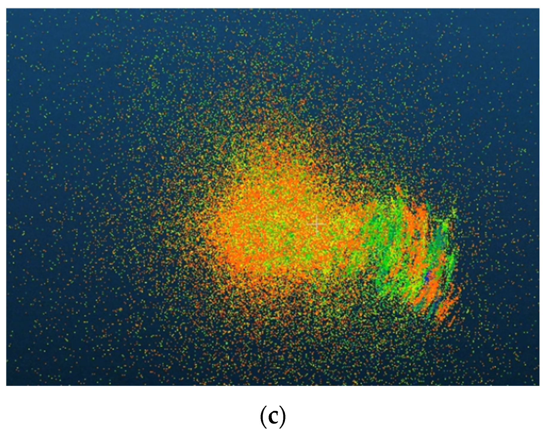
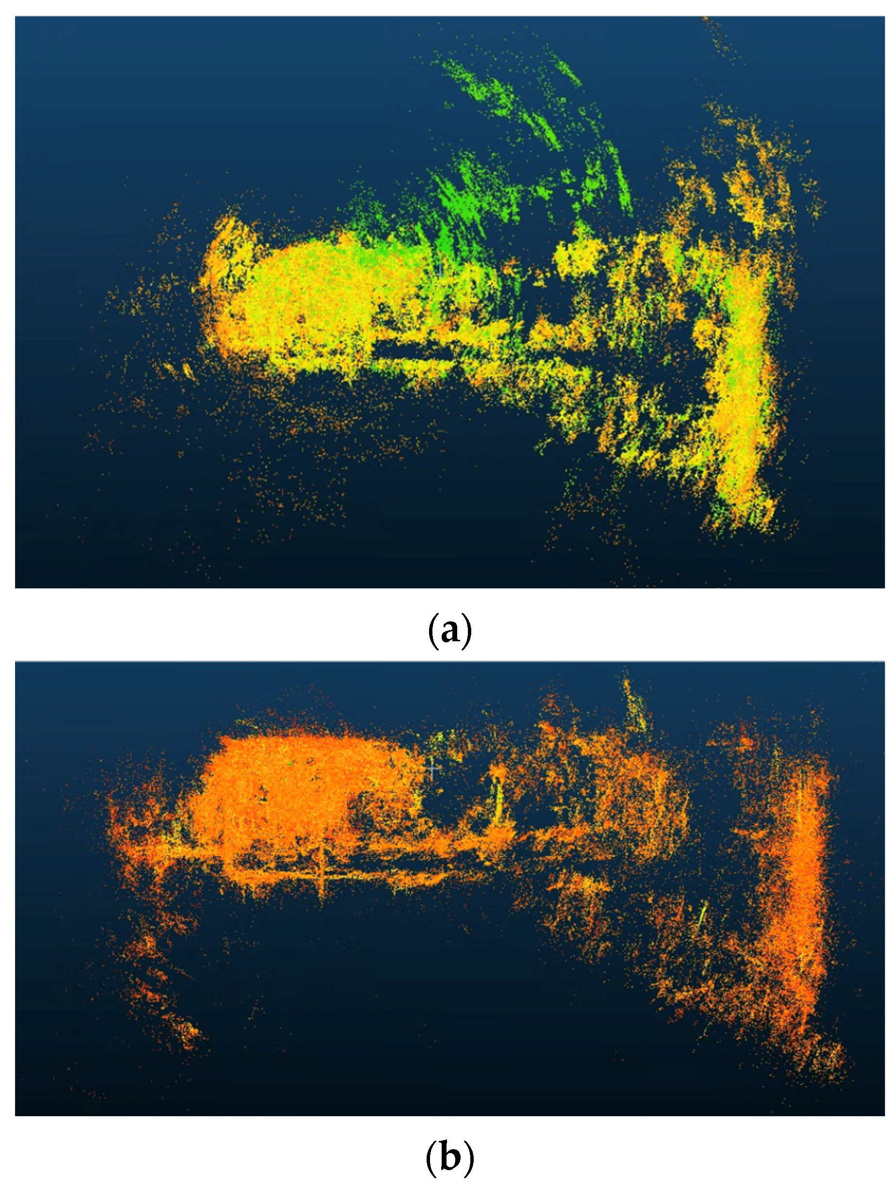
The main problem when dealing with the results from PostShot is that the splats form a sort of “sphere” around the object surveyed that is composed of noisy data that must be cancelled. This can interfere with the accuracy of the data (Figure 5a–c). The noisiest is MCMC since by default it reconstructs more details of the surroundings.

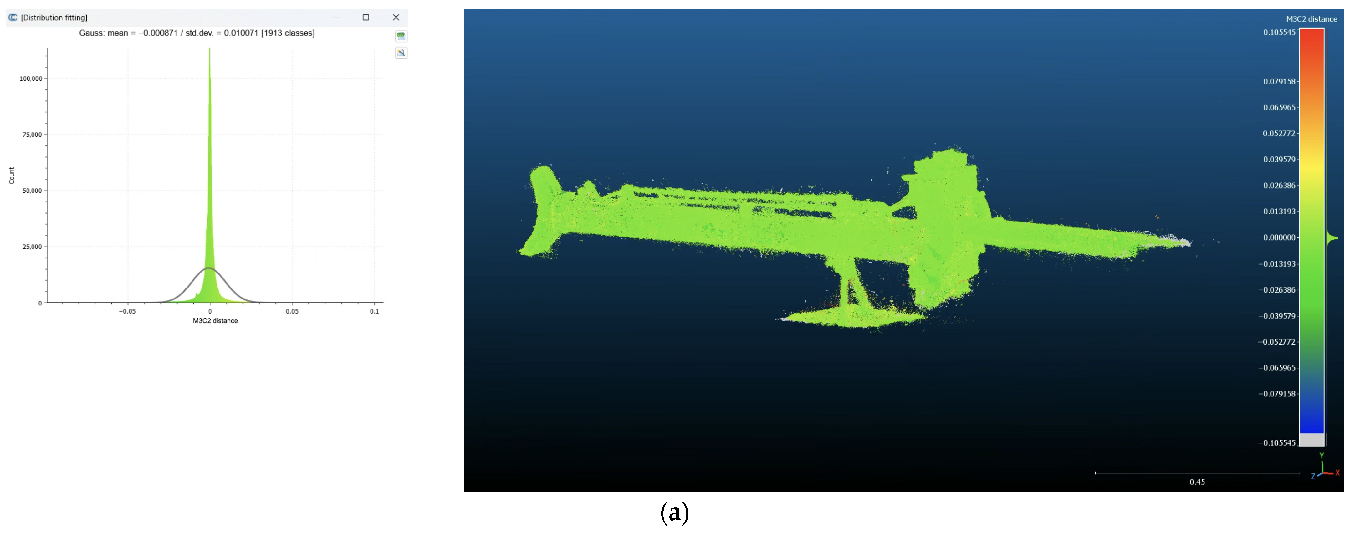
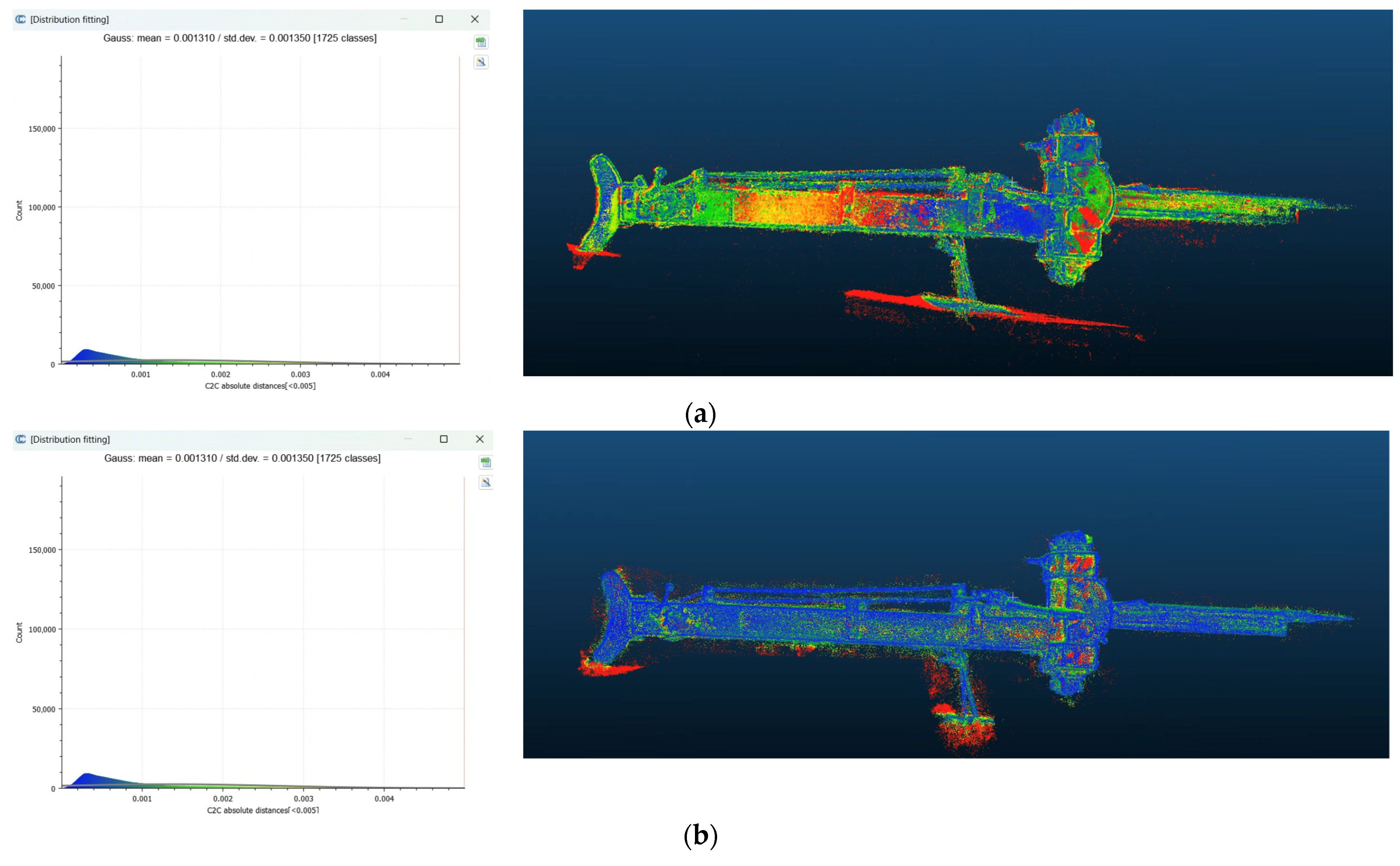
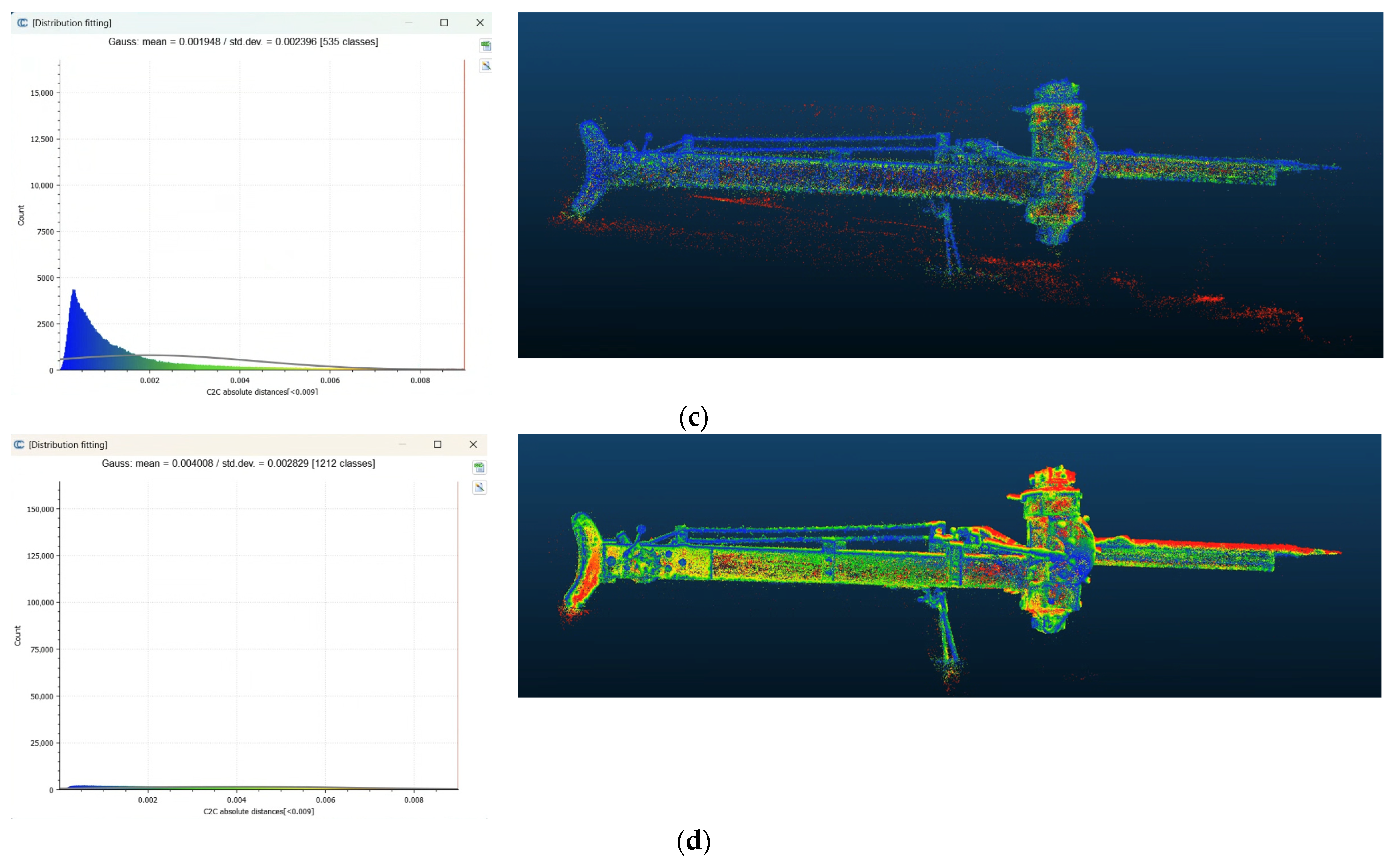
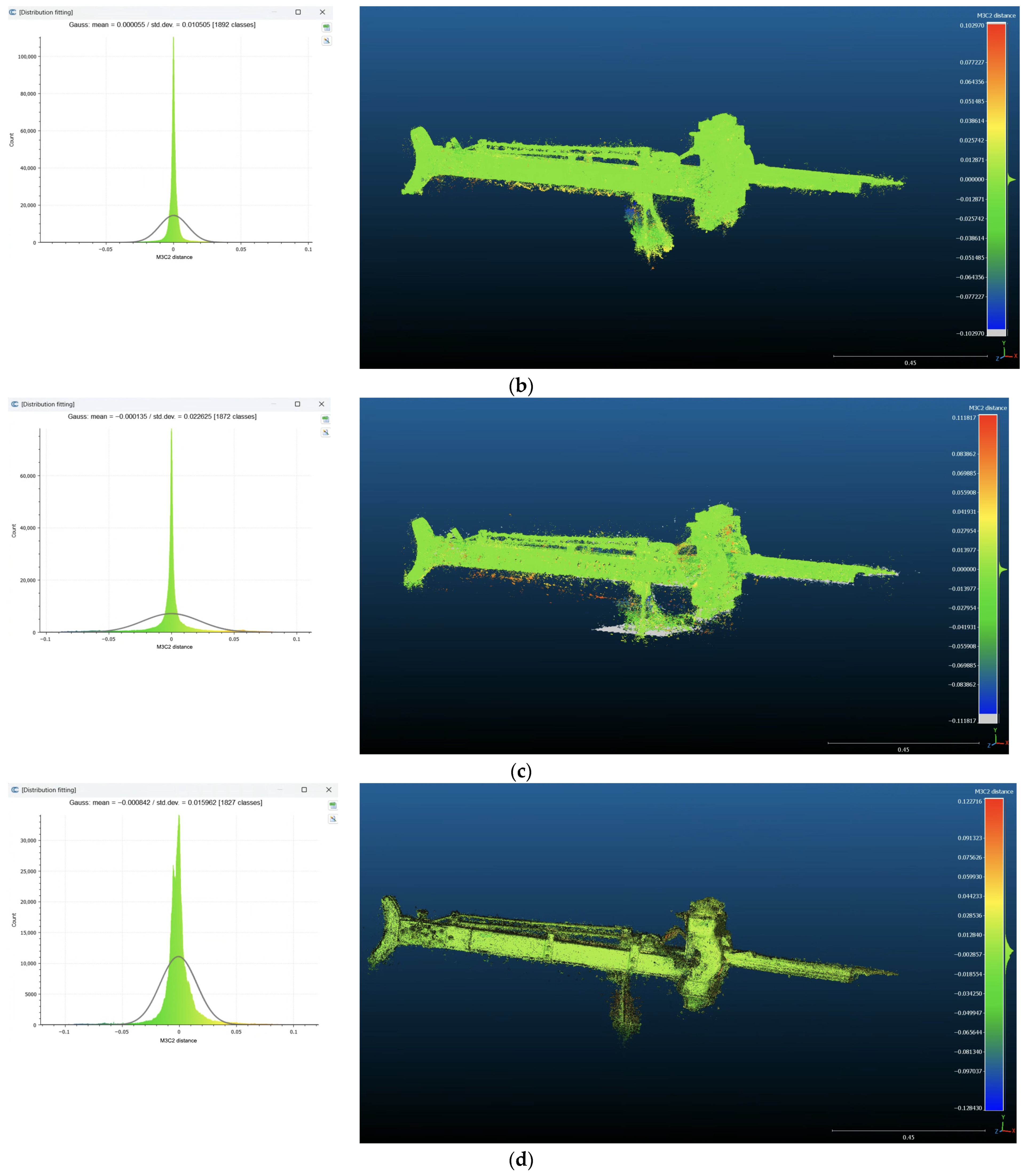
The following step involved the comparison of each 3D point cloud/splat with the Metashape 2.2.1 one. The results are visible in Figure 6a–d and are summarised in

Table 2. Comparison of Metashape 2.2.1 point cloud with 3DGS and Colmap 3.14 data using the M3C2 tool. The mean and standard deviation are expressed in metres.

Software	Mean	Standard Deviation
Colmap	−0.0009	0.01
3DGS SPLAT3	0.00006	0.011
3DGS SPLAT ADC	−0.00014	0.023
3DGS SPLAT MCMC	−0.0008	0.016

.

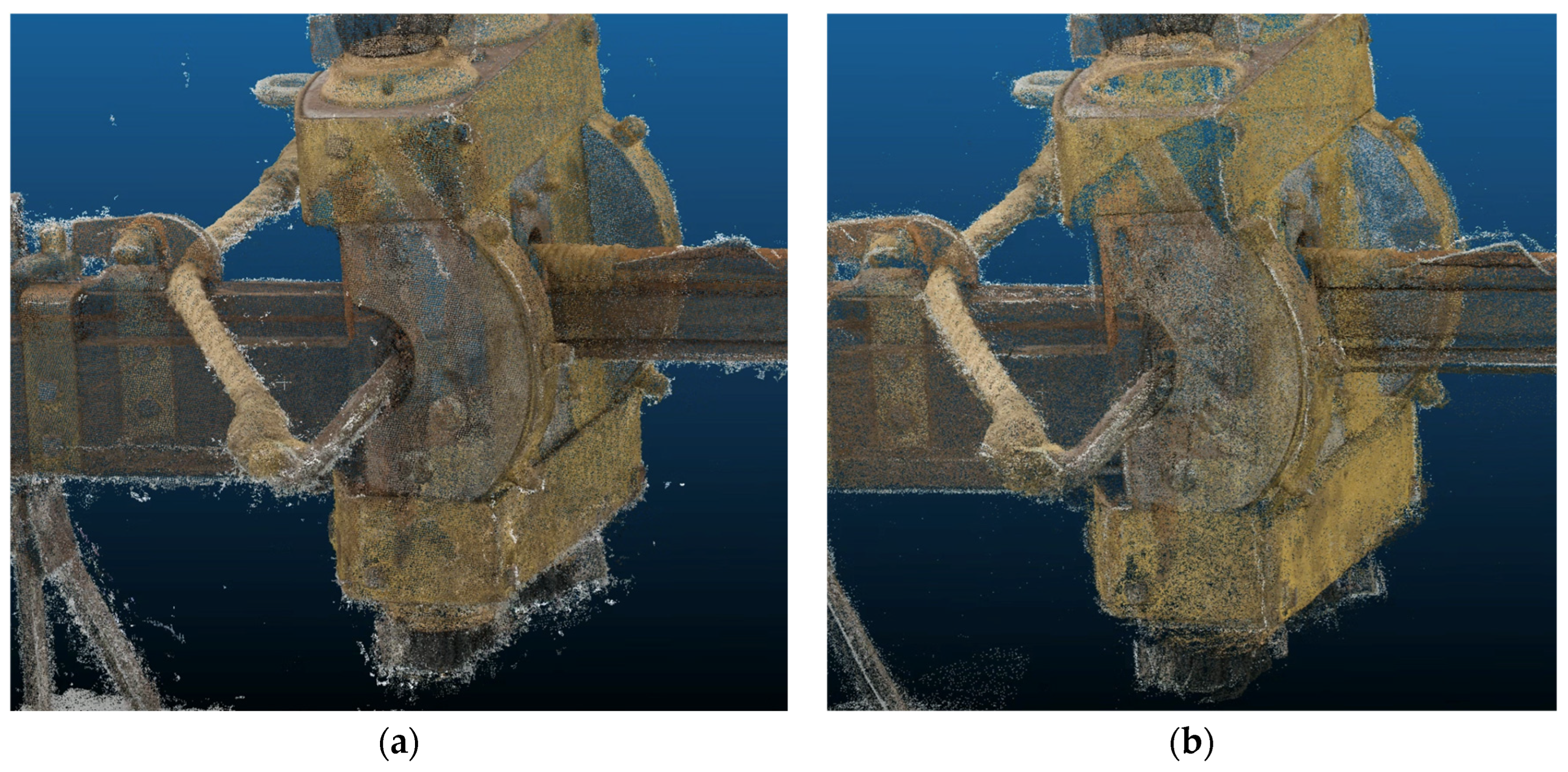
Again, the worst result was the one using SLAP3 ADC parameters, while MCMC gave a slightly higher standard deviation than SPLAT3 and Colmap 3.14. The latter surprisingly gave a standard deviation of 1 cm, probably since the point cloud is sparser than the one of Metashape 2.2.1, and hence the details are less visible (Figure 7a,b).

The comparison of the 3D data using the C2C tool gave different results, as expected (

Table 3. Comparison of Metashape 2.2.1 point cloud with 3DGS and Colmap 3.14 data using the C2C tool. The mean and standard deviation are expressed in metres.

Software	Mean	Standard Deviation
Colmap	0.0013	0.0014
3DGS SPLAT3	0.0013	0.0014
3DGS SPLAT ADC	0.002	0.0024
3DGS SPLAT MCMC	0.004	0.003

and Figure 8a–d).

Just simply visually, it can be noticed that the calculation of distances is different, and the distribution of the Gaussian (bell curve) describing the distance error or local surface variance is not perfectly shaped (e.g., skewed, flattened, bimodal, or having heavy tails). This can indicate that the data does not follow a simple, random “normal” distribution. This is common when comparing point clouds and refers usually to structural or systematic issues rather than just random noise.

The cause may be that one side of the object has more points closer to the model, while the other side is further away. This often happens in photogrammetry where lighting variations cause structural deformation in the generated mesh. A non-uniform density or surface curvature (flattened/broadened), as in the case of the comparison using the C2C tool, may be caused by the low density of one of the two point clouds, while high outlier presence (heavy tails/fat tails) means that the “tails” of the bell curve are too thick, indicating that many points exist far from the mean. This can result from the noise of the point cloud, like environmental artefacts, or incomplete cleaning (denoising). These outliers skew the standard deviation, making it seem like the entire cloud is less precise than it is.

The big difference between the standard deviation calculations in the comparison is because the two tools perform calculations in different ways. M3C2 often delivers a higher standard deviation because it is a more complex, robust, and physically accurate algorithm that unambiguously describes local surface roughness and noise. C2C simply calculates the shortest distance between points, while M3C2 computes signed distances along local normal vectors within a defined projection cylinder.

The reasons why the standard deviation calculated in M3C2 is often higher are:

• Sensitivity to Local Roughness (Normal Orientation): Since M3C2 relies on accurate surface normals to calculate distances, high surface roughness or noisy normals in the data can influence the calculation, leading to a larger range of distances, increasing the standard deviation.
• Measurement of Real Variation vs. Smoothing: C2 can smooth out differences while M3C2 captures real, smaller-scale variations in surface topography.
• Projection Cylinder Effects: M3C2 uses a cylinder to find points in the other cloud. If the cylinder diameter (D) is fixed too wide, it may include points that are not on the same surface, creating a wider distribution of distances.
• Incorporation of Noise in Statistical Calculation: Uncertainty and standard deviation are calculated based on local point density and noise. If the clouds are noisy, M3C2 will correctly report a higher standard deviation, whereas C2C might just show a simple noisy distance.
• Core Points Subsampling: M3C2 often uses a subsampled subset of “core points” to represent the cloud. If the core point cloud is not representative of the whole, or if the subsampling is too sparse in high-gradient areas, it can impact the statistics.

5. Conclusions

The present research’s goal was to analyse the accuracy of Gaussian Splatting data compared to SfM point clouds to understand if they can be used as models for structural analysis with FEA. The methodology followed a specific, well-established pipeline, using the same data for 3DGS processing as input, with external and internal orientation calculated in Colmap 3.14. In this way, the starting point for each training of data was the same. We also decided to use the Agisoft Metashape 2.2.1 point cloud as reference since this data has been used as a basis for the processing of meshes and volumes used in FEA. So, it was assumed that the accuracy of this data was good enough for the purpose.

The resulting 3D data was compared using two different tools in CloudCompare 2.13.2 to have a better comprehension of the data obtained. Analysing the solutions of the comparison, it can be stated that, considering the Cloud-to-Cloud distance calculation, 3DGS SPLAT3 shows a standard deviation equal to that of Colmap, while ADC is a little higher and MCMC is worse. This is mainly due to the fact that the latter setting is less suitable for the reconstruction of small details and complex geometry. The same results were obtained using the M3C2 tool; even in this case, ADC data resulted in the worst outcomes. Considering the different procedures used by these two tools to analyse discrepancies in point cloud comparison, the poor quality of the Gaussian distribution shown in C2C states that the noise in all the 3DGS data can strongly influence the result of the comparison. Manual cleaning is not sufficient and may introduce discrepancies. With the M3C2 tool, the standard deviation increased strongly, which indicates that the sparse reconstruction given by Gaussian Splatting platform PostShot is not as accurate as SfM point clouds.

The next step of the research will be to test other platforms of scripts and to try to create a mesh from Gaussian Splatting data to analyse it, applying retopology and then importing the volume into FEA software to see if the model can be analysed.

References

1. Mildenhall, B.; Srinivasan, P.P.; Tancik, M.; Barron, J.T.; Ramamoorthi, R.; Ng, R. Nerf: Representing scenes as neural radiance fields for view synthesis. Commun. ACM 2021, 65, 99–106. [Google Scholar] [CrossRef] [Scilit]
2. Fei, B.; Xu, J.; Zhang, R.; Zhou, Q.; Yang, W.; He, Y. 3D Gaussian Splatting as a New Era: A Survey. IEEE Trans. Vis. Comput. Graph. 2025, 31, 4429–4449. [Google Scholar] [CrossRef] [Scilit] [PubMed]
3. Ye, V.; Li, R.; Kerr, J.; Turkulainen, M.; Yi, B.; Pan, Z.; Seiskari, O.; Ye, J.; Hu, J.; Tancik, M.; et al. gsplat: An Open-Source Library for Gaussian Splatting. arXiv 2024, arXiv:2409.06765. [Google Scholar] [CrossRef] [Scilit]
4. Billi, D.; Caroti, G.; Piemonte, A. 3D Reconstruction of Transparent and Reflective Surfaces, Through the Use of SfM Processes Supported by 3D Gaussian-Splatting and 2D Gaussian-Splatting. Preprints 2025, 2025052191. [Google Scholar] [CrossRef] [Scilit]
5. Gonizzi Barsanti, S.; Guagliano, M.; Rossi, A. 3D Reality-Based Survey and Retopology for Structural Analysis of Cultural Heritage. Sensors 2022, 22, 9593. [Google Scholar] [CrossRef] [Scilit] [PubMed]
6. Lyu, X.; Sun, Y.T.; Huang, J.H.; Wu, X.; Yang, Z.; Chen, Y.; Pang, J.; Qi, X. 3DGSR: Implicit Surface Reconstruction with 3D Gaussian Splatting. ACM Trans. Graph 2024, 43, 198. [Google Scholar] [CrossRef] [Scilit]
7. Wu, T. Recent Advances in 3D Gaussian Splatting. arXiv 2024, arXiv:2403.11134. [Google Scholar] [CrossRef] [Scilit]
8. Ye, Z.; Li, W.; Liu, S.; Qiao, P.; Dou, Y. Abs3DGS: Recovering Fine Details in 3D Gaussian Splatting. In Proceedings of the 32nd ACM International Conference on Multimedia (MM ‘24), Melbourne, VIC, Australia, 28 October–1 November 2024; Association for Computing Machinery: New York, NY, USA, 2024; pp. 1053–1061. [Google Scholar] [CrossRef] [Scilit]
9. Ji, B.; Yao, A. SfM-Free 3D Gaussian Splatting via Hierarchical Training. In Proceedings of the IEEE/CVF Conference on Computer Vision and Pattern Recognition (CVPR), Nashville, TN, USA, 11–15 June 2025; pp. 21654–21663. [Google Scholar]
10. Yang, Q.; Yang, K.; Xing, Y.; Xu, Y.; Li, Z. A Benchmark for Gaussian Splatting Compression and Quality Assessment Study. In Proceedings of the 6th ACM International Conference on Multimedia in Asia (MMAsia ‘24); Association for Computing Machinery: New York, NY, USA, 2024; pp. 1–8. [Google Scholar] [CrossRef] [Scilit]
11. Sun, G.; Liu, D.; Yang, Z.; An, S.; Zhang, Y. 3D reconstruction and precision evaluation of industrial components via Gaussian Splatting. Comput. Graph. 2025, 132, 104422. [Google Scholar] [CrossRef] [Scilit]
12. Gao, L.; Yang, J.; Zhang, B.T.; Sun, J.M.; Yuan, Y.J.; Fu, H.; Lai, Y.K. Mesh-based Gaussian Splatting for Real-time Large-scale Deformation. arXiv 2024, arXiv:2402.04796. [Google Scholar] [CrossRef] [Scilit]
13. Sambugaro, Z.; Orlandi, L.; Conci, N. 3D reconstruction methods in industrial settings: A comparative study for COLMAP, NeRF and 3D Gaussian Splatting. In Proceedings of the 4th National Conference on Artificial Intelligence, organized by CINI (Ital-IA 2024), Naples, Italy, 29–30 May 2024; pp. 212–217. [Google Scholar]
14. Wu, Y.; Liu, K.; Zhang, L.; Chen, M.; Luo, Y.; Li, H.; Wang, L.; Cai, Y. Improving 3D Gaussian splatting for radiance field rendering using deep structure-from-motion. In Proceedings of the SPIE 13511, Tenth Symposium on Novel Optoelectronic Detection Technology and Applications, 1351106 (17 February 2025); SPIE: Bellingham, WA, USA, 2025. [Google Scholar] [CrossRef] [Scilit]
15. Fang, X.; Zhang, Y.; Tan, H.; Liu, C.; Yang, X. Performance Evaluation and Optimization of 3D Gaussian Splatting in Indoor Scene Generation and Rendering. ISPRS Int. J. Geo-Inf. 2025, 14, 21. [Google Scholar] [CrossRef] [Scilit]
16. Zhou, Y.; Zeng, Z.; Chen, A.; Zhou, X.; Ni, H.; Zhang, S.; Li, P.; Liu, I.; Zheng, M.; Chen, X. Evaluating Modern Approaches in 3D Scene Reconstruction: NeRF vs Gaussian-Based Methods. In Proceedings of the 2024 6th International Conference on Data-driven Optimization of Complex Systems (DOCS), Hangzhou, China, 16–18 August 2024; pp. 926–931. [Google Scholar] [CrossRef] [Scilit]
17. Fu, Y.; Wang, X.; Liu, S.; Kulkarni, A.; Kautz, J.; Efros, A.A. COLMAP-Free 3D Gaussian Splatting. In Proceedings of the 2024 IEEE/CVF Conference on Computer Vision and Pattern Recognition (CVPR), Seattle, WA, USA, 17–21 June 2024; pp. 20796–20805. [Google Scholar] [CrossRef] [Scilit]
18. Yu, Y.; Verbree, E.; van Oosterom, P.; Pottgiesser, U.; Peng, Y.; Poux, F. From comparison to integration: A workflow evaluation of 3D Gaussian splatting and LiDAR point cloud for modern architectural heritage. Autom. Constr. 2025, 180, 106509. [Google Scholar] [CrossRef] [Scilit]
19. Jamil, O.; Brennan, A. Immersive heritage through Gaussian Splatting: A new visual aesthetic for reality capture. Front. Comput. 2025, 7, 1515609. [Google Scholar] [CrossRef] [Scilit]
20. Kwon, O.; Yu, J. Realistic and Interactive Virtual Museum Representation Using 3D Gaussian Splatting. ISPRS Ann. Photogramm. Remote Sens. Spat. Inf. Sci. 2025, X-M-2-2025, 185–192. [Google Scholar] [CrossRef] [Scilit]
21. Lee, J.; Park, S.; Min, J.; Choi, J. 3D Gaussian Splatting for Enhanced Documentation of Cultural Artifacts. ISPRS Ann. Photogramm. Remote Sens. Spat. Inf. Sci. 2025, X-M-2-2025, 215–222. [Google Scholar] [CrossRef] [Scilit]
22. He, Y.; Zhang, X.; Xie, Z.; Li, D.; He, J.; Chen, R. A dual-prior driven Gaussian splatting framework for high-fidelity reconstruction of museum artifacts. npj Herit. Sci. 2026, 14, 69. [Google Scholar] [CrossRef] [Scilit]
23. Jia, Q.; He, J. High-fidelity 3D reconstruction of cultural heritage via super-resolution and progressive Gaussian splatting. npj Herit. Sci. 2026, 14, 84. [Google Scholar] [CrossRef] [Scilit]
24. Clini, P.; Nespeca, R.; Angeloni, R.; Coppetta, L. 3D representation of Architectural Heritage: A comparative analysis of NeRF, Gaussian Splatting, and SfM-MVS reconstructions using low-cost sensors. Int. Arch. Photogramm. Remote Sens. Spat. Inf. Sci. 2024, XLVIII-2/W8-2024, 93–99. [Google Scholar] [CrossRef] [Scilit]
25. Murtiyoso, A.; Macher, H. Gaussian Splatting for Facade Orthophoto Generation—Comparison with MVS and TLS. Int. Arch. Photogramm. Remote Sens. Spat. Inf. Sci. 2025, XLVIII-M-9-2025, 1059–1064. [Google Scholar] [CrossRef] [Scilit]
26. Tanduo, B.; Matrone, F.; Murtiyoso, A. Initial Experiments on the Use of Radiance Fields for Underwater 3D Reconstruction. Int. Arch. Photogramm. Remote Sens. Spat. Inf. Sci. 2025, XLVIII-M-9-2025, 1475–1481. [Google Scholar] [CrossRef] [Scilit]
27. Fang, G.; Wang, B. Mini-Splatting: Representing Scenes with a Constrained Number of Gaussians. In Computer Vision—ECCV 2024; Lecture Notes in Computer Science; Leonardis, A., Ricci, E., Roth, S., Russakovsky, O., Sattler, T., Varol, G., Eds.; Springer: Cham, Switzerland, 2024; Volume 15135. [Google Scholar] [CrossRef] [Scilit]
28. Fratino, M.; Palmero Iglesias, L.; Rossi, A. Re-Construction of the Small Xanten-Wardt Dart Launcher. Eng. Proc. 2025, 96, 9. [Google Scholar] [CrossRef] [Scilit]
29. Gonizzi Barsanti, S. Denoising and voxelization for finite element analysis: A review. Eng. Proc. 2025, 96, 6. [Google Scholar] [CrossRef] [Scilit]
30. Becker, D.; Raddatz, L.; Roussel, C.; Klonowski, J. Analysis methods for deformation detection using TLS and UAS data on the example of a landslide simulation. Geo-Engineering 2024, 15, 9. [Google Scholar] [CrossRef] [Scilit]
Figure 1. The copy of the Scorpionide surveyed.
Engproc 149 00002 g001
Figure 2. The process in Agisoft Metshape 2.2.1: (a) the position of the acquired images; (b) the resulting point cloud.
Engproc 149 00002 g002
Figure 3. The retopologised mesh (a) and a detailed view of the quadrangular elements (b).
Engproc 149 00002 g003
Figure 4. The 3D data: (a) Metashape 2.2.1; (b) Colmap 3.14; (c) SLAPT3; (d) ADC; (e) MCMC.
Engproc 149 00002 g004aEngproc 149 00002 g004b
Figure 5. The raw results of PostShot: (a) Spalt3; (b) ADC; (c) MCMC.
Engproc 149 00002 g005aEngproc 149 00002 g005b
Figure 6. Comparison of Metashape 2.2.1 3D point cloud with (a) Colmap 3.14; (b) 3DGS SPLAT3; (c) 3DGS ADC; and (d) 3DGS MCMC using the M3C2 tool in CloudCompare 2.13.2.
Engproc 149 00002 g006aEngproc 149 00002 g006b
Figure 7. Comparison of Metashape 2.2.1 3D point cloud (a) and Colmap 3.14 (b).
Engproc 149 00002 g007
Figure 8. Comparison of Metashape 2.2.1 3D point cloud with (a) Colmap 3.14; (b) 3DGS SPLAT3; (c) 3DGS ADC; and (d) 3DGS MCMC using the C2C tool in CloudCompare 2.13.2.
Engproc 149 00002 g008aEngproc 149 00002 g008b