Compensations for Horizontal Inertial Components of INS/GNSS with Flight Altitude ^†

Abstract

This research examines the fundamental autonomous inertial navigation formulas for aircraft. The study aims to identify analytical errors arising from the use of approximate gravity field models and proposes corrections for horizontal inertial components relative to changes in flight altitude. GPS measurements of ground speed and its total and relative derivatives are transformed into compensations for Coriolis and centrifugal accelerations, with flight altitude taken into account. This type of compensation corresponds to a precisely defined gravitational field model, assumed to be accurate to the second degree of eccentricity.

1. Introduction

The autonomous inertial method for determining the speed and location of a moving object is based on the use of information about two vectors: $\overrightarrow{g}$, the relative gravitational force, and $\overrightarrow{\Omega }$, the angular velocity of the Earth’s daily rotation. Sensitive elements are inertial sensors: accelerometers and gyroscopes. In this work, the object of study is the values of $\overrightarrow{g}$, present in the accelerometer readings. This is a priori information, specified in flight at the current geodetic latitude B and altitude above the ellipsoid h. The goal is to show how, when introducing $\overrightarrow{g}(B,h)$ into the equations of inertial navigation, it is possible to separate constantly acting components. Conventional navigation algorithms feature methodological errors, some of which are smaller than the instrumental errors of the accelerometers. Their consideration in navigation tasks is necessary to achieve high accuracy, comparable to that of global radio navigation systems. This is possible only in the presence of highly sensitive accelerometers.

As is known, the total acceleration of a moving point in a moving coordinate system is the algebraic sum of three accelerations: transport, relative and Coriolis. When moving in near-Earth space, the transport acceleration is the centrifugal acceleration resulting from the diurnal rotation of the Earth. The force of inertia resulting from this acceleration, together with the attractive force of the Earth’s gravitational field, form the force of weight. Accelerometers respond to the movement of their body in absolute inertial space (relative to the stars).

2. Essence of the Problem

The vector $\overrightarrow{g}$ cannot be measured in flight. Instead, accelerometers measure the apparent acceleration $\overrightarrow{a}$, which is the difference between the full acceleration $\overrightarrow{\varpi }$ and gravitation acceleration $\overrightarrow{g}$: $\overrightarrow{a}=\overrightarrow{\varpi }-\overrightarrow{g}$. 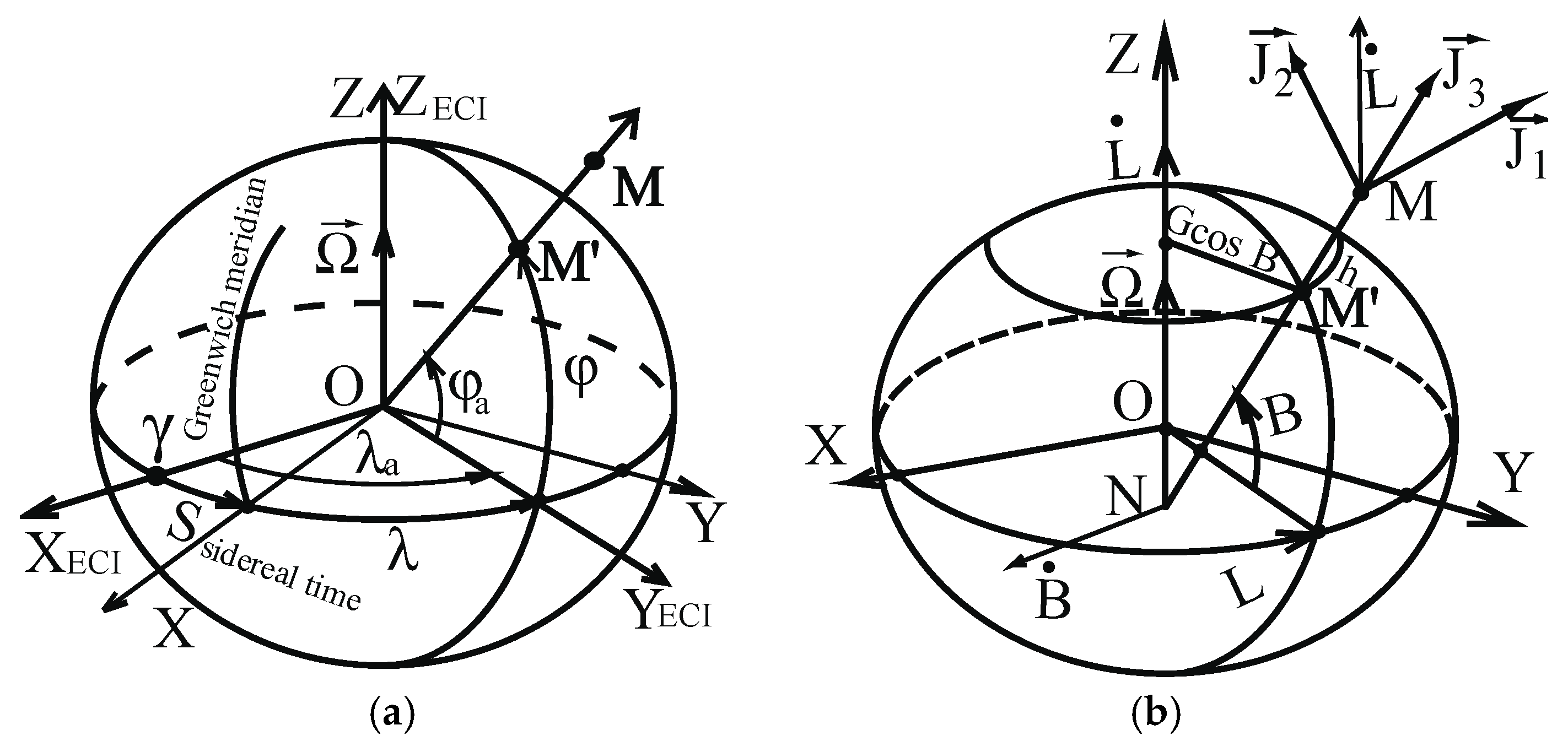The inertial acceleration $\overrightarrow{\varpi }(t)$ is the derivative of the inertial velocity vector $\overrightarrow{V}(t)$ in the ECI coordinate system (Figure 1) [1]:

$$\overrightarrow{\varpi }(t)={\displaystyle \frac{d}{dt}}\overrightarrow{V}(t),$$

(1)

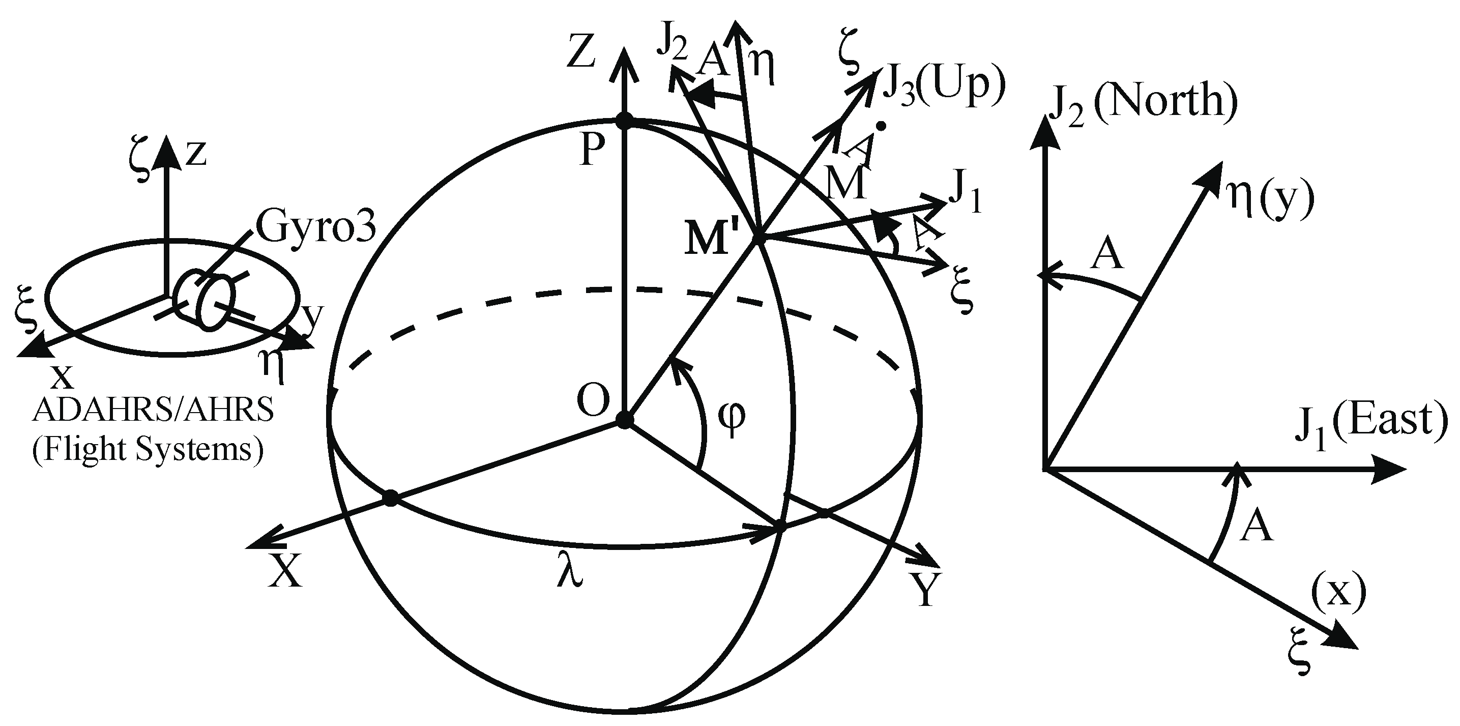
In the navigation coordinate system ξηζ (Figure 2) [2], the first form for accelerometer measurements is:

$$\overrightarrow{a}=\overrightarrow{\varpi }-\overrightarrow{g}=\dot{\overrightarrow{V}}+{\overrightarrow{\omega }}^a\overrightarrow{V}-\overrightarrow{g}.$$

(2)

where ${\overrightarrow{\omega }}^a$ is the inertial angular velocity vector, and $\overrightarrow{g}(B,h)$ is present immediately.

Inertial navigation sensors have their own instrumented coordinate system, which, depending on the implementation, is an electromechanical gyro platform or a body-fixed (strapdown INS): AHRS (Attitude and Heading Reference System) is a system using sensors (gyroscopes, accelerometers) to provide attitude and heading data to pilots, commonly found in modern aircraft; ADAHRS (Air Data, Attitude and Heading System) is a critical, advanced electronic system used in light sport, ultralight and experimental aircraft to provide flight data (altitude, speed, attitude). All coordinate systems are right-handed, with one axis up.

The inertial sensors are placed at the center of mass of the aircraft, point M, which is the origin of the coordinates. These systems have a certain orientation relative to the directions of the world, given by a coordinate system with axes tangent to the local meridian and parallel: the local, point-M’ Cartesian coordinate system (ENU) with unit vectors ${\overrightarrow{J}}_1(East)$, ${\overrightarrow{J}}_2(North)$, ${\overrightarrow{J}}_3(Up)$ (Figure 2) [2].

There is also a second form of the equation for representing accelerometer measurements, which apparently involves the projections $W_x,W_y,W_z$ of the velocity vector $\overrightarrow{W}$ relative to the ground, rather than the projections $V_x,V_y,V_z$ of the inertial velocity vector $\overrightarrow{V}$. For the total acceleration [2,3] from the theory of inertial navigation, the representation is known to be

$$\overrightarrow{\varpi }=\dot{\overrightarrow{W}}+\overrightarrow{\omega }\times \overrightarrow{W}+2\overrightarrow{\Omega }\times \overrightarrow{W}+\overrightarrow{\Omega }\times (\overrightarrow{\Omega }\times \overrightarrow{R})$$

(3)

where: $\dot{\overrightarrow{W}}+\overrightarrow{\omega }\times \overrightarrow{W}$ represents the relative accelerations, $2\overrightarrow{\Omega }\times \overrightarrow{W}$ is Coriolis accelerations, and $\overrightarrow{f}=-\overrightarrow{\Omega }\times (\overrightarrow{\Omega }\times \overrightarrow{R})$ is the transport (centrifugal) acceleration. In this form of representation, $\overrightarrow{R}$ is the distance from the center of mass of the Earth O to the center of mass M of the aircraft or the position vector (Figure 1), $\overrightarrow{W}$ is the ground speed vector and $\overrightarrow{\Omega }$ is the Earth’s angular velocity. Relative acceleration is represented in two terms. The first $\dot{\overrightarrow{W}}$ is the derivative of the ground speed, considered in a coordinate system moving relative to the Earth. As such, the reference navigation basis with axes ξηζ and its adopted and its relative angular velocity $\overrightarrow{\omega }$ can be calculated absolutely accurately, without methodological errors, taking into account the geometric shape of the Earth as a rotating ellipsoid. The second term $\overrightarrow{\omega }\times \overrightarrow{W}$ essentially takes into account the curvature of the aircraft’s trajectory in space.

The vector equation

$$\dot{\overrightarrow{W}}=\overrightarrow{a}-\overrightarrow{\omega }\times \overrightarrow{W}-2\overrightarrow{\Omega }\times \overrightarrow{W}+\overrightarrow{g}-\overrightarrow{\Omega }\times (\overrightarrow{\Omega }\times \overrightarrow{R})$$

(4)

is used to calculate the projections of the ground speed. The separation of the relative and Coriolis accelerations from the accelerometer measurements as deterministic components (Eötvös effect) is visible [4]. The relative force of weight (per unit mass) is taken as

$${\overrightarrow{g}}^T=\overrightarrow{g}+\overrightarrow{f}=\overrightarrow{g}-\overrightarrow{\Omega }\times (\overrightarrow{\Omega }\times \overrightarrow{R}).$$

(5)

To calculate the value of ${\overrightarrow{g}}^T$, an accepted standard model for $\overrightarrow{g}(B,h)$ is used [5]. The centrifugal acceleration is added, after calculation, with a known position vector $\overrightarrow{R}$ with geodetic latitude B, geodetic latitude L and height h above the ellipsoid (Figure 1b). Accordingly, the geocentric coordinates of point M are (φ, λ, R) (Figure 1a).

International Gravity Standardization Formulas

The latest update to World Geodetic System (WGS 84) is known as WGS 84 (G2296) (dated March 2024), and is aligned with the International Terrestrial Reference System ITRF2022. This is the seventh such update using Global Positioning System (GPS) measurements in 30 years. The current version, WGS 84, defines an ECEF coordinate system and a geodetic datum, and also describes the associated Earth Gravitational Model (EGM) and World Magnetic Model (WMM) [5]. The basic constants (parameters) that define the WGS84 (World Geodetic System 1984) reference ellipsoid are a = 6,378,137 m—semi-major axis; 1/f = 298.257223563—flattening factor of the Earth; GM = 3.986004418 × 10⁺¹⁴ m³/s²—geocentric gravitation constant; γ_e = 9.7803253359 m/s²—normal gravity at the Equator; γ_p = 9.8321849379 m/s²—normal gravity at the Pole; e² = 0.006694379990141; ω $\equiv \Omega$ = $\left|\overrightarrow{\Omega }\right|$ = 7.292115 × 10⁻⁵ rad/s—nominal mean angular velocity of the Earth (Figure 1):

$$q=\left(a{\Omega }^2\right)/{\gamma }_e=0.003467748240693.$$

(6)

The International Gravity Formula of 1967 (IGF67), part of the Geodetic Reference System of 1967 (GRS67), defines the Earth’s normal gravitational acceleration γ(B) at sea level as a function of latitude B. It replaces the older 1930 standard, providing more accurate measurements based on more recent satellite data. These formulas are expressed as follows [5] (Somigliana’s formula):

$$\gamma \left(B,h=0\right)={\gamma }_e\left(1+\beta {\sin }^{2}B+{\beta }_1{\sin }^{2}2B\right)$$

(7)

The international formula for gravity, 1930, with improved values by Sir Harold Jeffreysin, 1948, per [6,7], is as follows: ${\gamma }_e$ = 9.780373 m/s²; β = 5.2891 × 10⁻³; β₁ = −5.9 × 10⁻⁶.

The International Gravity Formula of 1967 (IGF 67), part of the Geodetic Reference System 1967 (GRS67), is ${\gamma }_e$ = 9.780318 m/s²; β = 5.3024 × 10⁻³; β₁ = −5.9 × 10⁻⁶.

The International Gravity Formula of 1967 (IGF 80), part of the Geodetic Reference System 1967 (GRS80), is ${\gamma }_e$ = 9.780327 m/s²; β = 5.3024 × 10⁻³; β₁ = −5.8 × 10⁻⁶.

With GRS 80, the following decomposition into a series is also introduced:

$$\gamma \left(B,h=0\right)={\gamma }_e\left(1+c_1{\sin }^{2}B+c_2{\sin }^{4}B+c_3{\sin }^{6}B+c_4{\sin }^{8}B\right),$$

(8)

where c₁ = 5.2790414 × 10⁻³; c₂ = 2.32718 × 10⁻⁵; c₃ = 1.262 × 10⁻⁷; c₄ = 7 × 10⁻¹⁰. Their accuracy is about ±10⁻⁶ m/s² and they are valid for the level of the rotational ellipsoid.

3. The Horizontal Components of the Gravitational Field in a First Approximation

When flying at low altitudes, it is permissible [2] to assume first-order values of the gravitational field on the surface of the reference ellipsoid e²:

North component:

$$g_N=0.5g_e^{T}q\sin 2B=a{\Omega }^2\sin B\cos B$$

(9)

Vertical component (+ is Up):

$$g_n=g_3=-g_e^T\left[1+q-2{\displaystyle \frac{h}{a}}+{\displaystyle \frac{1}{2}}(3q-e^2){\sin }^{2}B\right].$$

(10)

They specify the intensity of the Earth’s gravitational field as a function of the geodetic latitude B and the height h above the ellipsoid (Figure 1). Using the geoid [4] as a zero surface is inconvenient due to its complex analytical form. In aviation, its first approximation is adopted as a rotational ellipsoid. By definition, this is a surface to which the force of gravity is normal at every point. For the zero surface, the force of weight, as a function of the geocentric latitude φ, is generally considered to be

$$g_n^T=-g_e^T\left[1-2(h/a)+\beta {\sin }^2\phi \right].$$

(11)

The difference $\mu =B-\phi \approx 0.5e^2\sin 2\phi \approx 0.5e^2\sin 2B$ between the geocentric φ and geodetic latitudes B and the distance from a point on the reference ellipsoid to the center of the Earth are taken as $R=a(1-0.5e^2{\sin }^2\phi )\approx a(1-0.5e^2{\sin }^{2}B)$ in the first approximation; therefore, from (10), the force of gravity at zero height is [8]:

$$g_n^T=-g_e^T(1+\beta {\sin }^{2}B), \beta ={\displaystyle \frac{5}{2}}q-{\displaystyle \frac{e^2}{2}}=\left({\displaystyle \frac{2}{2}}+{\displaystyle \frac{3}{2}}\right)q-{\displaystyle \frac{e^2}{2}}.$$

(12)

If we compare the accepted standard representations (12) for weight and (10) for gravity,

$$g_n=-g_e^T\left[1+(q-q{\sin }^{2}B)-2{\displaystyle \frac{h}{a}}+{\displaystyle \frac{1}{2}}(5q-e^2){\sin }^{2}B\right],$$

(13)

we will notice that the north projection $g_N=a{\Omega }^2\sin B\cos B$ and the component in the vertical projection $-g_e^T(q-q{\sin }^{2}B)=-g_e^{T}q{\cos }^{2}B=-a{\Omega }^2{\cos }^{2}B$ of the gravity model (9), (13) take into account centripetal acceleration. Such values of centripetal acceleration exist at points on a sphere with radius a.

When flying at a height h above a rotating ellipsoid, the radius of the first vertical is $G=a\xi +h$, $\xi ={\left(1-e^2{\sin }^{2}B\right)}^{-1/2}$. For this, the centrifugal acceleration from the Earth’s rotation is

$$\overrightarrow{f}=-\overrightarrow{\Omega }\times (\overrightarrow{\Omega }\times \left(\begin{array}{c}0\\ 0\\ G\end{array}\right))=\left(\begin{array}{c}0\\ -{\Omega }^{2}G\cos B\sin B\\ {\Omega }^{2}G\cos B\cos B\end{array}\right).$$

(14)

From (9), (12) and (14) for a standard value of the acceleration of free fall from a height h, we obtain

$${\overrightarrow{g}}^T=\left(\begin{array}{c}{g}_E^T\\ g_N^T\\ g_n^T\end{array}\right)=\left(\begin{array}{c}0\\ {\Omega }^2(a-a\xi -h)\cos B\sin B\\ -g_e^T(1-2{\displaystyle \frac{h}{a}}+\beta {\sin }^{2}B)-{\Omega }^2(a-a\xi -h){\cos }^{2}B\end{array}\right),$$

(15)

where its projections onto the navigation datum ξηζ can be represented according to the accepted notations:

$$\begin{gathered} {\overrightarrow{g}}^T=\left(\begin{array}{c}{g}_{\xi }^T\\ g_{\eta }^T\\ g_{\zeta }^T\end{array}\right)=\left(\begin{array}{c}-g_N^T\sin A\\ g_N^T\cos A\\ g_n^T\end{array}\right)=\left(\begin{array}{c}-{\Omega }^2(a-a\xi -h)\sin A\cos B\sin B\\ {\Omega }^2(a-a\xi -h)\cos A\cos B\sin B\\ g_n^T\end{array}\right)= \\ \left(\begin{array}{c}{\Omega }^2(a-a\xi -h)u_{13}{u}_{33}\\ {\Omega }^2(a-a\xi -h)u_{23}{u}_{33}\\ -g_e^T(1-2{\displaystyle \frac{h}{a}}+\beta u_{33})-{\Omega }^2(a-a\xi -h)(1-u_{33}^2)\end{array}\right), \end{gathered}$$

(16)

where $u_{13}=-\sin A\cos B,u_{12}=\cos A\cos B,u_{33}=\sin B,u_{13}^2+u_{23}^2+u_{33}^2=1$ and A is the azimuth of the instrumental direction η (Figure 2), $\beta =\left(5q-e^2\right)/2$ = 5.322180606663169 × 10⁻³.

This model should be used in the inertial navigation Equations (4) and (5). Its accuracy corresponds to the first degree of approximation in the transition between a sphere and a rotational ellipsoid. In it, the consideration of the radius of curvature of the meridian ellipse is of particular importance. It partially compensates for the Eötvös effect, which manifests itself due to the non-sphericity of the Earth.

4. Compensation of Horizontal Inertial Components in INS by GNSS Ground Speed Measurements

The GPS measurement method gives Cartesian ECEF projections of ground speed $\overrightarrow{W}$. Their conversion to the reference navigation basis with axes ξηζ for inertial speed $\overrightarrow{V}$ and from there to total acceleration $\overrightarrow{\varpi }$ (1) is required. The conversion is done by taking into account inertial corrections (Eötvös effect and free air anomaly [4,9] and requires the calculation of projections into ECEF of inertial angular velocity ${\overrightarrow{\omega }}^a$ into a moving navigation basis ξηζ.

The vector ${\overrightarrow{\omega }}^a=\overrightarrow{\Omega }+\overrightarrow{\omega }$ sums the diurnal rotation of the Earth with $\overrightarrow{\Omega }$ and the rotation of ξηζ relative to it $\overrightarrow{\omega }$. It is the sum of relative $\overrightarrow{\omega }$ and transport $\overrightarrow{\Omega }$ angular velocities. For the total acceleration $\overrightarrow{\varpi }$, there are several equivalent forms (1) or (3), each of which has its specific application. To show their equivalence, the differentiation of $\overrightarrow{V}=\overrightarrow{W}+\overrightarrow{\Omega }\times \overrightarrow{R}$ is used in the following sequence of transformations:

$$\begin{gathered} \overrightarrow{\varpi }={\displaystyle \frac{d\overrightarrow{V}}{dt}}={\displaystyle \frac{\tilde{d}\overrightarrow{V}}{dt}}+{\overrightarrow{\omega }}^a\times \overrightarrow{V}={\displaystyle \frac{\tilde{d}\overrightarrow{W}}{dt}}+{\displaystyle \frac{d\overrightarrow{\Omega }}{dt}}\times \overrightarrow{R}+\overrightarrow{\Omega }\times \overrightarrow{W}+{\overrightarrow{\omega }}^a\times \overrightarrow{V}= \\ {\displaystyle \frac{\tilde{d}\overrightarrow{W}}{dt}}-\overrightarrow{\omega }\times \overrightarrow{\Omega }\times \overrightarrow{R}+\overrightarrow{\Omega }\times \overrightarrow{W}+{\overrightarrow{\omega }}^a\times \overrightarrow{V}= \end{gathered}$$

(17)

$$\begin{gathered} {\displaystyle \frac{\tilde{d}\overrightarrow{W}}{dt}}-\overrightarrow{\omega }\times \overrightarrow{\Omega }\times \overrightarrow{R}+\overrightarrow{\Omega }\times \overrightarrow{W}+\overrightarrow{\omega }\times \overrightarrow{W}+\overrightarrow{\omega }\times \overrightarrow{\Omega }\times \overrightarrow{R}+\overrightarrow{\Omega }\times \overrightarrow{W}+\overrightarrow{\Omega }\times \overrightarrow{\Omega }\times \overrightarrow{R}= \\ {\displaystyle \frac{\tilde{d}\overrightarrow{W}}{dt}}+\overrightarrow{\omega }\times \overrightarrow{W}+2\overrightarrow{\Omega }\times \overrightarrow{W}+\overrightarrow{\Omega }\times \overrightarrow{\Omega }\times \overrightarrow{R}. \end{gathered}$$

(18)

Inertial velocity and total acceleration have the following projections in ξηζ:

$$\begin{array}{l}{V}_{\xi }=W_{\xi }+(a\xi +h)\Omega u_{23},\hfill \\ V_{\eta }=W_{\eta }-(a\xi +h)\Omega u_{13},\hfill \\ V_{\zeta }=W_{\zeta },\hfill \end{array}$$

(19)

$$\begin{array}{l}{\varpi }_{\xi }={\dot{W}}_{\xi }+(a\dot{\xi }+\dot{h})\Omega u_{23}+(a\xi +h)\Omega {\dot{u}}_{23}+{\omega }_{\eta }^a{V}_{\zeta }-{\omega }_{\zeta }^a{V}_{\eta },\hfill \\ {\varpi }_{\eta }={\dot{W}}_{\eta }-(a\dot{\xi }+\dot{h})\Omega u_{13}-(a\xi +h)\Omega {\dot{u}}_{13}-{\omega }_{\xi }^a{V}_{\zeta }+{\omega }_{\zeta }^a{V}_{\xi },\hfill \\ {\varpi }_{\zeta }={\dot{W}}_{\zeta }+{\omega }_{\xi }^a{V}_{\eta }-{\omega }_{\eta }^a{V}_{\xi }.\hfill \end{array}$$

(20)

After laborious transformations, the identities are proven:

$$\begin{array}{l}a\dot{\xi }\Omega u_{23}+(a\xi +h)\Omega {\dot{u}}_{23}=-\Omega u_{33}{W}_{\eta },\\ -a\dot{\xi }\Omega u_{13}-(a\xi +h)\Omega {\dot{u}}_{13}=\Omega u_{33}{W}_{\xi }.\end{array}$$

(21)

These are horizontal projections of a part of the Coriolis acceleration, arising when taking into account the non-sphericity of the Earth. Their participation in the form (17) for total acceleration is seen after representing the vectors in scalar form:

$$\overrightarrow{\Omega }\times \overrightarrow{W}=\left(\begin{array}{c}{W}_{\zeta }\Omega u_{23}\\ -W_{\zeta }\Omega u_{13}\\ -\Omega (W_{\xi }{u}_{23}-W_{\eta }{u}_{13})\end{array}\right)-\overrightarrow{\omega }\times \overrightarrow{\Omega }\times \overrightarrow{R}=\left(\begin{array}{c}a\dot{\xi }\Omega u_{23}+(a\xi +h)\Omega {\dot{u}}_{23}\\ -a\dot{\xi }\Omega u_{13}-(a\xi +h)\Omega {\dot{u}}_{13}\\ \Omega (W_{\xi }{u}_{23}-W_{\eta }{u}_{13})\end{array}\right)=\left(\begin{array}{c}-\Omega u_{33}{W}_{\eta }\\ \Omega u_{33}{W}_{\xi }\\ \Omega (W_{\xi }{u}_{23}-W_{\eta }{u}_{13})\end{array}\right).$$

(22)

The final conclusion is that in (18) and (20), the Coriolis acceleration is fully taken into account, regardless of the form in which the absolute acceleration is calculated. However, this is not the case when taking into account the centripetal acceleration $\overrightarrow{\Omega }\times \overrightarrow{\Omega }\times \overrightarrow{R}$, when the height above the reference ellipsoid is introduced, i.e., $\overrightarrow{R}$ is taken along the geodesic vertical and has a module $a\xi +h$, and for the model gravitational field the projections (9) and (10) are:

$$\overrightarrow{g}=\left(\begin{array}{c}{g}_{\xi }\\ g_{\eta }\\ g_{\zeta }\end{array}\right)=\left(\begin{array}{c}a{\Omega }^2{u}_{13}{u}_{33}\\ a{\Omega }^2{u}_{23}{u}_{33}\\ -g_e^T[1+q-2{\displaystyle \frac{h}{a}}+0.5(3q-e^2)u_{33}^2]\end{array}\right).$$

(23)

In this case, there are inertial components in the projections ξηζ of the total acceleration, uncompensated components depending on the height above the ellipsoid and more precisely on the difference between the geocentric and geodetic verticals:

$$\begin{array}{l}{\varpi }_{\xi }={\dot{W}}_{\xi }+({\omega }_{\eta }+2\Omega u_{23})W_{\zeta }-({\omega }_{\zeta }+2\Omega u_{33})W_{\eta }+{\Omega }^2(a\xi +h)u_{13}{u}_{33},\\ {\varpi }_{\eta }={\dot{W}}_{\eta }-({\omega }_{\xi }+2\Omega u_{13})W_{\zeta }+({\omega }_{\zeta }+2\Omega u_{33})W_{\xi }+{\Omega }^2(a\xi +h)u_{23}{u}_{33},\\ {\varpi }_{\zeta }={\dot{W}}_{\zeta }+({\omega }_{\xi }+2\Omega u_{13})W_{\eta }-({\omega }_{\eta }+2\Omega u_{23})W_{\xi }-{\Omega }^2(a\xi +h)(1-u_{33}^2).\end{array}$$

(24)

Compensation is possible when (13) is taken as the vertical component of the gravitational field, in the manner shown in (16). With this conclusion, compensation for the horizontal inertial components in the INS has been achieved through GNSS ground velocity measurements.

5. Discussion and Conclusions

Despite the equivalence of the two forms of representation of the basic equations of inertial navigation, full compensation for the constant components in the accelerometer measurements is not guaranteed. In the second form, the inertial component of the Earth’s rotation increases with altitude.

An original method for its approximate compensation, using a simplified model of the gravitational field, has been found here. Reference [10] presents two gravity compensation methods using the Earth Gravitational Model 2008 (EGM2008), namely interpolation from an off-line database and direct computation of the gravity vectors using the spherical harmonic model. Here, the time duration for calculating the current gravity vector using EGM2008 has been reduced to less than 1 s by optimizing the calculation procedure. The safety certification of GNSS-assisted inertial navigation systems (INS) in civil aircraft requires rigorous testing to ensure proper operation, even under the worst conditions. One error that must be considered is that of gravity compensation in accelerometer measurements, and Reference [11] describes a method for determining effective stochastic error models of current high-order gravity models, such as EGM2008.

For the geodetic latitude B from the tables, the values of centrifugal acceleration from Earth’s rotation ${\Omega }^{2}a\cos B\sin B$ and ${\Omega }^{2}a{\cos }^{2}B$ can be found in

Table 1. Values of centrifugal acceleration from Earth’s rotation (14).

B [deg]	15	30	45	60	75
${\Omega }^{2}a\cos B\sin B$ [mGal]	847.89	1468.6	1695.8	1468.6	847.89
${\Omega }^{2}a{\cos }^{2}B$ [mGal]	3164.4	2543.7	1695.8	847.89	227.19

:

Table 2. Correction of ${\Omega }^2(a-a\xi -h)\cos B\sin B$ [mGal] [10⁻⁵ m/s²] in the Northern channel for measured accelerations $\overrightarrow{a}=\overrightarrow{\varpi }-\overrightarrow{g}$.

B [deg]	h[m]0	500	1000	1500	2000	2500	3000
15	−0.38048	−0.44695	−0.51342	−0.57989	−0.64636	−0.71283	−0.7793
30	−2.464	−2.5791	−2.6943	−2.8094	−2.9245	−3.0397	−3.1548
45	−5.7048	−5.8377	−5.9706	−6.1036	−6.2365	−6.3695	−6.5024
60	−7.4295	−7.5446	−7.6597	−7.7749	−7.89	−8.0051	−8.1203
75	−5.346	−5.4125	−5.479	−5.5454	−5.6119	−5.6784	−5.7448

and

Table 3. Correction of ${\Omega }^2(a-a\xi -h){\cos }^{2}B$ [mGal] [10⁻⁵ m/s²] in the vertical channel for measured accelerations $\overrightarrow{a}=\overrightarrow{\varpi }-\overrightarrow{g}$.

B [deg]	h[m]0	500	1000	1500	2000	2500	3000
15	−1.42	−1.668	−1.9161	−2.1642	−2.4122	−2.6603	−2.9084
30	−4.2678	−4.4672	−4.6666	−4.866	−5.0654	−5.2648	−5.4642
45	−5.7048	−5.8377	−5.9706	−6.1036	−6.2365	−6.3695	−6.5024
60	−4.2894	−4.3559	−4.4224	−4.4888	−4.5553	−4.6218	−4.6882
75	−1.4325	−1.4503	−1.4681	−1.4859	−1.5037	−1.5215	−1.5393

show the values of the inertial components, which are added to the horizontal and vertical components of gravitation to obtain the projections of the acceleration of free fall (15).

The values in Table 2 and Table 3 allow us to assess the effectiveness of reducing the relative error after the introduced corrections. If another model for representing the gravity field is used, such as those described in (7) and (8), it is necessary to look for another adequate way to introduce corrections in the horizontal channels. Similar types of corrections are needed in algorithms of autonomous Quantum IMUs with NV diamond sensors. Nitrogen-Vacancy (NV) diamond accelerometers are emerging quantum sensors that use diamond lattice imperfections to measure acceleration, offering high sensitivity, low power consumption, and miniaturization potential for GPS-denied navigation [12]. The comparison in sensitivity and size of some representative gyroscopes and the NV-based gyroscope is shown in [12], including ring laser gyroscope (RLG), fiber optical gyroscope (FOG), spin relaxation free (SERF) gyroscope, atom interferometer gyroscope (AIG), micro-electro-mechanical systems (MEMS) gyroscope, and NV-based gyroscope. As a new type of atomic gyroscope, the NV-based gyroscope has the potential for medium sensitivity (10⁻⁶ rad/s/$\sqrt{Hz}$) and miniaturization in the future.

The instability of the vertical channel cannot be eliminated with approximate mathematical models of gravity, but it is possible to reduce the height error with an appropriate selection of a gravity field model. This model must also be consistent with the possibility of compensating for the inertial components in height. GNSS measurements allow for partial estimation and correction of horizontal inertial corrections before flight according to (24) [13].

For electromechanical systems, the difference between the geocentric and geodetic vertical has a positive effect on achieving stability in controlling the gyro platform. In strapdown INS, this difference increases the methodological errors of the inertial method.