Fault-Aware Decision Support for Renewable-Powered EV Charging Stations Using Multi-Source Explainable Learning

Abstract

Electric vehicle charging stations (EVCSs) are increasingly deployed as grid-interactive energy assets that combine power electronic converters, sensing devices, communication interfaces, photovoltaic (PV) generation, battery energy storage systems (BESS), and multiple charging ports. This complexity creates reliability challenges because abnormal behavior may originate from electrical, thermal, sensing, communication, port-level, or grid-side sources. This paper proposes a fault-aware decision-support framework for renewable-powered EVCSs using multi-source explainable learning. The framework integrates electrical, thermal, session/port, grid/PV/BESS, and communication/data-quality indicators into a unified health-monitoring representation. Supervised models diagnose known fault classes, anomaly-detection models flag unknown or anomalous events, and a source-level explainability layer supports candidate-source interpretation and maintenance-oriented risk mapping. A scenario-controlled EVCS benchmark is developed with PV generation, BESS operation, grid import, charging-port behavior, communication/data-quality indicators, and six injected fault/anomaly categories. An extended 180-day benchmark further assesses longer-horizon operation, seasonal/weather diversity, drift/ageing proxies, and event-level behavior. The strongest closed-set classifier, LightGBM with class weights, achieved 98.45% accuracy and 0.9792 macro-F1, while the Random Forest model used for explainability and decision-layer analysis achieved 97.35% accuracy and 0.9626 macro-F1. Full multi-source monitoring improved Random Forest macro-F1 from 0.6922 under electrical-only monitoring to 0.9626, demonstrating within the controlled benchmark the diagnostic value of heterogeneous EVCS observability. Open-set performance was source dependent: sensor/measurement and communication/data anomalies were more detectable, whereas thermal/cooling and port/session unknowns remained difficult at the selected threshold. Under nominal scenario-based response assumptions, unavailable port hours and unmet charging energy decreased by 49.01% and 38.33%, respectively, relative to reactive operation; sensitivity analysis showed that these outcomes depend on intervention effectiveness and response delay. These findings establish controlled-benchmark feasibility for explainable multi-source EVCS decision support. Field validation using charger telemetry, maintenance-confirmed labels, and operator-calibrated response policies remains necessary.

1. Introduction

Electric vehicle charging stations (EVCSs) are increasingly becoming grid-interactive energy assets rather than passive charging loads. Modern stations may combine photovoltaic (PV) generation, battery energy storage systems (BESS), power electronic converters, multiple charging ports, local sensors, communication interfaces, and energy-management controllers [1,2,3,4]. This integration improves flexibility and can support renewable utilization, peak-load reduction, and smart-charging operation. However, it also changes the reliability problem: a charging station fault is no longer only an electrical event, but may affect service availability, local energy management, grid exchange, and maintenance response.

This creates a multi-source fault-risk problem across electrical, thermal, charging-session, port-level, communication/data-quality, PV, BESS, and grid-side layers. From the user perspective, failed charge initiation, interrupted charging sessions, unavailable ports, damaged connectors, communication failures, and unclear charger status directly reduce trust in public charging infrastructure. Field evidence has shown that user-facing charger availability may be lower than nominal network-reported uptime, with nonfunctional chargers affected by several hardware, interface, and operational causes [5]. Vehicle-side battery abnormalities may also affect station safety during charging, as thermal or electrical battery incidents can expose nearby charging equipment and users to secondary hazards; however, vehicle-battery diagnosis remains outside the primary scope of this study. From the operator and grid perspectives, abnormal operation may increase maintenance cost, reduce service availability, affect transformer loading and voltage quality, alter BESS dispatch, and reduce the dependability of local energy-management decisions.

Existing studies address important parts of this problem, but usually not the integrated decision-support problem. Converter and charging-pile faults have been investigated using signal-processing features, machine-learning classifiers, and spatiotemporal or multifeature fusion methods [6,7,8,9]. Sensor and measurement faults have been studied using observer-based residual analysis and adaptive thresholds [10]. Anomaly-detection methods have also been applied to charging profiles, thermal behavior, and cyber-physical EVCS monitoring [11,12,13,14,15,16]. These studies show that data-driven methods can detect abnormal EVCS behavior, but many of them stop at classification accuracy, F1-score, anomaly score, or detection time. In parallel, renewable-powered EVCS and microgrid studies often optimize PV utilization, BESS operation, grid import, cost, or emissions under the assumption that the charging infrastructure is healthy [3,4,17].

The specific research gap addressed in this paper is therefore the gap between accurate EVCS fault detection and practical, source-aware, explainable, maintenance-oriented decision support under renewable-powered operation. A useful EVCS decision-support framework should not only identify that an abnormal condition exists. It should also indicate which monitoring source provides the strongest evidence, whether the event resembles a known or unknown fault, how the diagnostic output maps into maintenance-oriented risk states, and how the resulting decision could affect service-level and grid-interactive indicators such as port availability, unmet charging energy, PV use, BESS response, and grid import.

This paper contributes a controlled benchmark and decision-support framework for this problem. The objective is not to propose a new charger topology, converter-control method, BESS dispatch optimizer, or field-validated maintenance product. Instead, the paper develops a reproducible multi-source machine-learning benchmark and uses it to evaluate how EVCS diagnostic outputs can be connected to source-level explanations, maintenance-oriented risk states, and scenario-based operational-response indicators. This controlled-benchmark approach is motivated by the lack of public datasets that jointly provide synchronized PV generation, BESS operation, electrical measurements, thermal indicators, port/session states, communication/data-quality variables, grid-side disturbances, and labeled maintenance faults in one unified schema [13,18,19,20,21,22]. The resulting claims are therefore interpreted as controlled-benchmark evidence, not as direct field-deployment performance.

The main contributions of this paper are as follows:

• A multi-source EVCS health-monitoring representation is developed for renewable-powered, grid-interactive charging stations by combining electrical, thermal, session/port, grid/PV/BESS, and communication/data-quality indicators within a unified diagnostic feature space.
• A controlled fault-aware benchmark and evaluation protocol are introduced to assess closed-set diagnosis, feature-source ablation, open-set unknown-fault detection, mixed-fault behavior, and explanation consistency under repeatable EVCS operating conditions.
• A decision-support layer translates diagnostic outputs into candidate-source evidence, maintenance-oriented risk states, and scenario-based operational indicators, including port availability, unmet charging energy, and grid/DER-aware response measures.

These contributions can be distinguished as conceptual/methodological and practical. The conceptual and methodological contribution is an integrated EVCS health-management formulation that links heterogeneous station observability, known- and unknown-fault diagnosis, source-structured explanation, maintenance-oriented risk states, and renewable/grid-interactive response assessment. The practical contribution is a reproducible operator-support workflow that converts multi-source monitoring data into diagnostic labels, candidate fault sources, risk states, inspection priorities, and scenario-based service and DER indicators. The contribution is methodological rather than a new learning theorem, and its operational value is demonstrated only within the controlled benchmark.

The scope of this study is intentionally limited to controlled-benchmark evaluation. The injected fault signatures are physically interpretable and representative of major EVCS fault sources, but they are not calibrated field-failure distributions. Therefore, the reported results should be interpreted as evidence that the proposed multi-source framework is internally consistent and useful for studying fault-aware EVCS decision support under explicit simulation assumptions. Future work should validate the framework using field telemetry, OCPP event logs, charger fault codes, real maintenance records, and operator-specific response policies.

The remainder of this paper is organized as follows. Section 2 reviews related work on EVCS reliability, fault diagnosis, anomaly detection, renewable-powered charging, and maintenance decision support. Section 3 presents the proposed framework, scenario-controlled benchmark, monitored feature sources, diagnostic models, explainability layer, risk mapping, and operational-response assessment. Section 4 reports and discusses the experimental results, including closed-set diagnosis, feature-source ablation, open-set detection, explanation consistency, maintenance-oriented risk states, and scenario-based response outcomes. Section 5 concludes the paper and outlines directions for field validation and deployment-oriented extensions.

2. Related Work

2.1. EVCS Reliability and Fault Diagnosis

The reliability of electric vehicle charging stations (EVCSs) has become a critical issue as charging infrastructure expands from isolated charging units into networked, grid-interactive energy assets. Practical EVCS failures may arise from several sources, including power electronic converters, sensors, charging ports, connectors, communication modules, backend systems, and user-facing transaction processes. Field measurements have shown that public fast-charging reliability can be considerably lower than expected from nominal uptime indicators, with nonfunctional chargers affected by unresponsive interfaces, damaged hardware, failed charge initiation, payment issues, network faults, and connector problems [5]. These findings show that EVCS reliability is not limited to converter health; it is a station-level problem involving electrical, operational, and communication layers.

EV battery faults represent an adjacent safety concern because abnormal battery behavior during charging may expose the charging station, nearby equipment, vehicles, and personnel to secondary thermal and fire hazards. Charger-side measurements can also provide useful evidence for identifying battery abnormalities even when detailed onboard battery-management-system data are unavailable. Yang et al. [23] demonstrated this potential using a privacy-preserving personalized federated-learning framework trained on heterogeneous charging data collected from 10,154 EVs at 30 real charging stations. Their results show that station-collected charging sequences can support collaborative EV battery-fault warning without requiring raw data sharing among station operators or other data owners. This direction complements EVCS infrastructure monitoring by extending the charging station from a power-delivery asset to a potential observation point for vehicle-battery safety. The present study does not model vehicle-internal battery faults and should therefore not be interpreted as an EV battery-safety diagnostic framework. Its scope is limited to faults and anomalies originating in EVCS infrastructure and grid-interactive operation. A future extension could incorporate a separate vehicle/battery risk source using charger-side charging curves or privacy-preserving battery-health indicators, while retaining a clear distinction between vehicle-originated and station-originated abnormalities.

A substantial part of the EVCS fault-diagnosis literature focuses on power-electronic faults in DC charging piles. Open-circuit faults are particularly important because they may degrade power quality and charging performance without necessarily triggering conventional protection mechanisms. Chen et al. proposed a diagnostic approach based on an improved S-transform, principal component analysis, and LightGBM classification for open-circuit faults in DC charging stations [6]. Piao et al. used variational mode decomposition and an optimized support-vector-machine model for DC charging-pile open-circuit diagnosis [7]. More recent work has explored spatiotemporal and multifeature fusion, showing that combining temporal, frequency-domain, and spatial information can improve diagnosis under variable operating conditions [8,9].

Sensor and measurement faults form another important diagnostic category. Current and voltage sensors are essential for charger control, metering, protection, and condition monitoring. A sensor bias, drift, or failure may distort the apparent operating state and cause incorrect control or maintenance decisions. Huang et al. proposed an adaptive sliding-mode-observer method for current-sensor fault diagnosis in charging modules, using residuals and adaptive thresholds to distinguish different fault severities [10]. These studies provide valuable methods for specific converter and sensor faults. However, most remain focused on individual components or narrow fault classes, and their outputs are usually limited to diagnostic labels, accuracy, or detection time. They rarely connect the diagnosis to station-level health states, candidate-source interpretation, or maintenance-oriented operational response.

2.2. Anomaly Detection, Cyber-Physical Monitoring, and Explainability

Supervised fault classification is useful when known fault labels are available, but practical EVCS deployments may encounter rare or previously unseen abnormal events. This motivates anomaly-detection methods that can learn normal behavior and flag deviations without requiring a complete catalogue of predefined fault classes. Sakwa et al. proposed an autoencoder-based method for EV supply equipment monitoring and early fault detection using charging power profiles [11]. Thermal anomaly detection has also been investigated because high-power chargers and power-converter modules are exposed to repeated electrical and thermal stress. Gomez et al. developed a data-driven thermal model for detecting abnormal EVCS thermal behavior [12]. These studies highlight the value of data-driven monitoring beyond simple threshold-based protection.

Cyber-physical monitoring is also increasingly important because modern EVCSs depend on communication protocols, payment systems, remote station management, and backend platforms. Cyber or data-quality anomalies may lead to station unavailability, incorrect metering, false status reporting, delayed fault notification, or failed remote intervention. Recent studies have examined machine-learning-based cyberattack and anomaly detection for EVCS environments using multidimensional cyber-physical datasets, federated learning, and deep learning models [13,14,15,16]. Although cybersecurity is not the main focus of the present work, these studies show that communication and data-quality indicators should be considered part of EVCS health monitoring.

Explainability is required when diagnostic outputs are intended to support maintenance decisions rather than only report abnormality. Cederle et al. developed an explainable anomaly-detection framework for EV charging stations using feature-importance analysis to support interpretation of abnormal events [24]. This is important because an alarm dominated by electrical distortion, thermal residuals, failed sessions, or packet loss implies different maintenance actions. However, explainability in the EVCS literature is still often treated as a model-interpretation step rather than being explicitly linked to source-level diagnostic interpretation, risk scoring, and operational decision-making. The present study addresses this limitation by grouping diagnostic evidence according to monitoring source and using the resulting information to support maintenance-oriented decision states.

2.3. Renewable-Powered and Grid-Interactive EV Charging Stations

A parallel research stream investigates EVCS operation in renewable-powered and grid-interactive settings. Solar PV integration, battery energy storage, smart charging, and microgrid coordination can reduce grid dependency, lower emissions, and improve charging flexibility. Reviews of solar-powered EVCSs identify PV intermittency, BESS sizing, infrastructure cost, and grid impacts as important design challenges [1,25]. Bhatti et al. surveyed energy-management schemes for EVCSs and classified approaches across grid-connected, PV-assisted, storage-supported, centralized, decentralized, and aggregator-based configurations [2]. These studies show that EVCSs are increasingly treated as active energy-management systems rather than passive charging loads.

Optimization and simulation studies further demonstrate the role of renewable generation and storage in charging-station operation. Rehman et al. compared grid-only, grid-plus-PV, and grid-plus-PV-BESS charging scenarios and showed that renewable and storage integration can improve sustainability under suitable operating conditions [3]. Aldosari et al. optimized microgrid operation with EV charging, renewable generation, and BESS while considering cost and emissions [17]. Grid-aware co-simulation platforms such as EV-EcoSim provide useful tools for evaluating interactions among EV charging, PV, BESS, transformers, and distribution networks [4].

However, renewable-EVCS and grid-interactive studies usually assume that the charging infrastructure is healthy. They primarily evaluate energy-management objectives such as cost, emissions, grid import, transformer loading, PV utilization, or BESS operation. Faults in converters, sensors, thermal systems, ports, sessions, communication links, or station data streams are rarely integrated into the energy-management evaluation. This creates a separation between two important research directions: diagnostic studies that identify faults but often ignore grid-interactive operation, and renewable-EVCS studies that optimize operation but often ignore infrastructure degradation and maintenance. A fault-aware EVCS framework should connect these dimensions by evaluating diagnostic performance together with operational consequences such as port availability, unmet charging demand, and response latency.

2.4. Maintenance Decision Support and Remaining Gap

Predictive maintenance aims to move beyond reactive repair and fixed-interval preventive maintenance by using condition-monitoring data to identify abnormal behavior before it causes service disruption. In the EVCS domain, Cai et al. proposed a preventive-maintenance decision model for charging piles based on lifecycle optimization, safety failure probability, environmental factors, outage duration, and maintenance timeliness [26]. This work is important because it explicitly links charging-pile condition assessment to maintenance decisions. More generally, machine-learning methods have also been used for EV failure-mode prediction, battery fault detection, and RUL-aware EV fleet scheduling [27,28,29]. These studies show the value of early warning, health-aware scheduling, and degradation-sensitive operation.

Nevertheless, existing EVCS maintenance models are not yet fully integrated with real-time, multi-source diagnostic evidence. Preventive-maintenance studies often rely on age, lifecycle indicators, historical records, or optimization assumptions, while diagnostic studies often produce fault labels without translating them into maintenance states, risk levels, or operational actions.

External Dataset Compatibility and Validation Scope

Recent real-world EV and battery datasets provide complementary evidence for individual components of charging-station analysis. Li et al. [30] reported 909,135 DC fast-charging sessions from 612 chargers, providing charging-power, state-of-charge, duration, energy, connector, and location information that is useful for calibrating realistic charging-profile and demand variability. However, access to the complete dataset is subject to a non-disclosure agreement. Yang et al. [23] released 21,175 charging records containing 1,547,432 samples from 10,154 EVs across 30 charging stations for privacy-preserving vehicle-battery fault warning. The Changan large-scale battery dataset [31] similarly supports battery-health, degradation, remaining-life, and fault studies.

Table 1. Compatibility of recent real-world EV and battery datasets with the validation requirements of the proposed EVCS framework.

Dataset/Resource	Primary Task	Main Available Information	Alignment with This Study	Appropriate Validation Role
Li et al. [30]	DC fast-charging profile and duration prediction	Charging power and vehicle state-of-charge trajectories; connector type and rating; session duration; delivered energy; station location; ambient-temperature context	Partial alignment with session/port and charging-demand representation; no labeled EVCS infrastructure-fault classes or integrated PV/BESS variables	Calibration of charging-profile variability, session duration, connector-power distributions, and nominal demand-generation assumptions
Yang et al. [23]	Privacy-preserving EV battery-fault warning	Charger-collected voltage, current, power, temperature, state of charge, and battery-fault labels from heterogeneous stations and vehicles	Adjacent vehicle-battery safety task; labels are not equivalent to station converter, port, communication, cooling, or grid faults	Validation of a future vehicle-originated battery-risk source and cross-station transfer or federated-learning extensions
Changan large-scale battery dataset [31]	Battery health, degradation, remaining-life, and fault analysis	Real-world vehicle battery-operation measurements and battery-condition information	Battery-system rather than EVCS-infrastructure focus	Development or validation of a future battery-health and degradation module
Present controlled EVCS benchmark	Multi-source EVCS fault diagnosis and maintenance-oriented decision support	Electrical, thermal, session/port, grid/PV/BESS, communication/data-quality, and labeled EVCS fault information	Full alignment with the present framework, but simulation based	Integrated controlled evaluation of closed-set diagnosis, open-set detection, explanation, risk mapping, and operational response

summarizes the relevance of these resources to the present framework.

These datasets are not suitable for a direct external evaluation of the present seven-class classifier because their prediction targets, feature spaces, sampling structures, and labels differ from those of the controlled EVCS benchmark. In particular, the Li et al. dataset supports charging-profile and duration modeling, whereas the Yang et al. and Changan datasets primarily address vehicle-battery behavior. None jointly provides synchronized PV generation, BESS operation, EVCS electrical and thermal measurements, port/session states, communication/data-quality indicators, grid disturbances, and maintenance-confirmed station-fault labels. Consequently, direct comparisons of accuracy or macro-F1 would not be scientifically valid.

These resources instead support a staged validation pathway. First, real-world charging-profile data can be used to calibrate session duration, charger-power, and demand distributions in the benchmark generator. Second, battery-oriented datasets can support a separate vehicle-originated battery-risk module without conflating vehicle and station faults. Finally, full external validation of the proposed framework requires multi-site EVCS telemetry containing synchronized controller and OCPP logs, PV/BESS measurements, communication and data-quality indicators, protection events, maintenance-confirmed infrastructure faults, and intervention records.

Practical deployment also requires that diagnostic outputs be interpreted within relevant EVCS standards and communication frameworks. ISO 15118 defines vehicle-to-grid communication use cases, IEC 61851 specifies general conductive charging-system requirements, OCPP supports charge-point-to-backend communication and device management, and ISA/IEC 62443 provides a cybersecurity reference for networked industrial-control systems [32,33,34,35,36]. These standards do not prescribe a specific machine-learning algorithm, but they define the operational environment in which diagnostic and maintenance actions must be executed. Therefore, a useful EVCS decision-support framework should not evaluate diagnostic accuracy alone. It should also indicate the likely source of the abnormality, the confidence and persistence of the diagnostic evidence, and the expected operational impact under explicit response assumptions.

Table 2. Gap-oriented positioning of the proposed study relative to related EVCS research streams.

Research Stream	What It Solves	What Remains Missing	How This Paper Addresses It
Converter and sensor fault diagnosis	Detects specific electrical, converter, and measurement faults.	Usually component-specific and weakly linked to station-level decision support.	Embeds converter and sensor evidence within a multi-source EVCS health model.
Charging-profile, thermal, and cyber-physical anomaly detection	Identifies abnormal charging, thermal, communication, or data-quality behavior.	Often stops at anomaly scores without source-aware risk states or response logic.	Links anomaly detection to source-level explanation and maintenance-oriented risk mapping.
Renewable and grid-interactive EVCS operation	Optimizes PV, BESS, grid import, cost, emissions, and charging operation.	Usually assumes healthy charging infrastructure and excludes fault-aware maintenance.	Evaluates diagnosis and operational response in a renewable-powered EVCS setting.
Preventive and predictive maintenance models	Supports maintenance timing using lifecycle, outage, or health indicators.	Often weakly coupled with real-time electrical, thermal, session, grid, and communication evidence.	Translates multi-source diagnostic outputs into interpretable decision-support states.

summarizes the positioning of the present work relative to the main research streams. Existing studies provide strong foundations for converter diagnosis, sensor-fault detection, anomaly detection, renewable-EVCS operation, and preventive maintenance. The remaining gap is the lack of an integrated, multi-source, explainable, and fault-aware decision-support framework for renewable-powered EVCSs that jointly evaluates closed-set diagnosis, unknown-fault detection, source-level explanations, risk states, and scenario-based operational impact.

The distinction between the present study and earlier work is primarily one of scope and integration rather than a claim of universally higher classification accuracy. Existing studies have reported strong results for specific tasks, including converter open-circuit diagnosis, sensor-fault detection, charging-profile anomaly detection, explainable anomaly analysis, and lifecycle-based preventive-maintenance decisions. However, these tasks are typically evaluated separately and use different datasets, class definitions, and performance metrics. The present study instead evaluates whether closed-set diagnosis, unknown-event flagging, source-aware explanation, maintenance-oriented risk mapping, and renewable/grid-interactive response assessment can be connected within one reproducible EVCS benchmark. A quantitative and task-level comparison is provided in Section 4.7.1.

3. Proposed Framework and Benchmark

3.1. Framework Overview

This study develops a fault-aware decision-support framework for renewable-powered electric vehicle charging stations (EVCSs). The framework is designed to connect multi-source condition monitoring, diagnostic modeling, explainability, and maintenance-oriented operational assessment within a single evaluation pipeline. Unlike methods that treat EVCS diagnosis as an isolated classification problem, the proposed framework links diagnostic outputs to source-structured evidence and scenario-based operating responses.

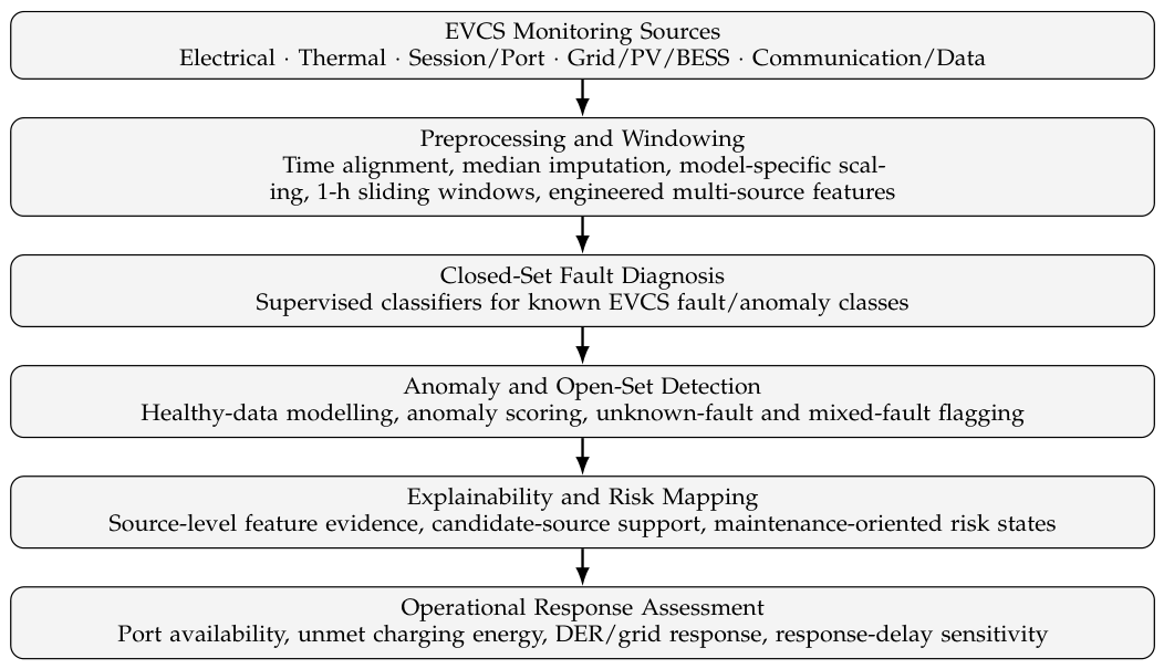
The framework consists of five main layers. The first layer represents the renewable-powered grid-interactive EVCS, including the grid connection, photovoltaic (PV) generation, battery energy storage system (BESS), charging ports, local sensors, and communication interfaces. The second layer generates and processes multi-source monitoring data from electrical, thermal, charging-session, port-level, grid/PV/BESS, and communication/data-quality sources. The third layer performs fault and anomaly diagnosis using supervised models for known fault classes and unsupervised or reconstruction-based models for unknown abnormal behavior. The fourth layer provides explainability and candidate-source support by grouping diagnostic evidence according to the monitored source. The fifth layer translates diagnostic outputs into health states, risk scores, and operational-impact indicators.

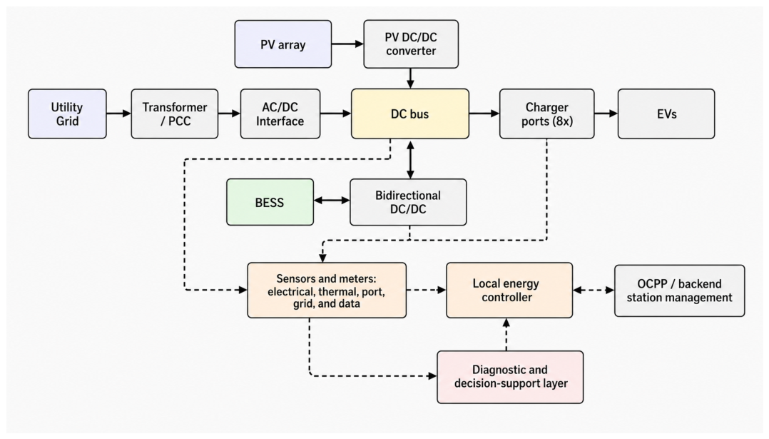
Figure 1 first provides the engineering context of the renewable-powered EVCS considered in this study. The architecture includes the utility-grid connection, transformer/PCC, AC/DC interface, PV generation, BESS, coupling interface, charger ports, EVs, local sensing and metering, OCPP/backend communication, local energy controller, and diagnostic decision-support layer. This architecture clarifies that the proposed framework is evaluated in a grid-interactive EVCS setting where electrical, thermal, session/port, communication/data-quality, PV/BESS, and grid-side variables are jointly relevant to fault-aware operation.

Figure 2 then summarizes the proposed fault-aware decision-support pipeline. Multi-source EVCS measurements are converted into window-based features and processed through closed-set fault classifiers, anomaly/open-set detectors, source-level explainability, maintenance-oriented risk mapping, and operational-response assessment. The two figures therefore separate the physical EVCS architecture from the data-driven decision-support workflow.

The study is implemented as a scenario-controlled simulation benchmark rather than as a field-deployed EVCS validation. This design enables repeatable evaluation of multiple fault sources under controlled assumptions, including converter faults, sensor faults, thermal/cooling anomalies, port/session failures, communication/data anomalies, and grid-side disturbances. Accordingly, the benchmark is used to evaluate the internal consistency and diagnostic usefulness of the proposed framework, not to claim direct field-deployment performance.

3.2. Renewable-Powered EVCS Architecture

The EVCS considered in this study consists of a grid connection, a local PV system, a BESS, multiple EV charging ports, local measurement devices, communication modules, and an energy-management controller. Energy can be supplied by the grid, local PV generation, or the BESS. When local PV generation exceeds the immediate charging and auxiliary demand, surplus PV can charge the BESS subject to power and state-of-charge limits. When PV generation is insufficient, the BESS may support charging demand and reduce grid import, depending on its available state of charge and power limit. This architecture is consistent with renewable-powered and grid-interactive EVCS studies in which charging load, local generation, storage, and grid exchange are treated as coupled operating variables [1,2,3,4]. The main technical assumptions used to configure the controlled EVCS benchmark are summarized in

Table 3. Main EVCS simulation configuration used in the controlled benchmark.

Parameter	Value
Simulation horizon	24 days
Sampling interval	5 min
Number of EV charging ports	8
Aggregate EVCS power rating	320 kW
Nominal grid-side voltage	400 V
PV capacity	180 kW
BESS capacity	350 kWh
Initial BESS SOC	0.55
BESS SOC range	0.15–0.90
Maximum BESS charge/discharge power	120 kW
BESS charge/discharge efficiency	0.95/0.95
Auxiliary station load	5 kW

.

The station-level power balance is expressed as

$$P_{\mathrm{grid}}\left(t\right)+P_{\mathrm{PV}}\left(t\right)+P_{\mathrm{BESS}}\left(t\right)=P_{\mathrm{EV}}\left(t\right)+P_{\mathrm{aux}}\left(t\right)+P_{\mathrm{loss}}\left(t\right).$$

(1)

where $P_{\mathrm{grid}}\left(t\right)$ is the grid-import power, $P_{\mathrm{PV}}\left(t\right)$ is the PV power used by the station, $P_{\mathrm{BESS}}\left(t\right)$ is the net BESS power, $P_{\mathrm{EV}}\left(t\right)$ is the aggregate EV charging power, $P_{\mathrm{aux}}\left(t\right)$ is the auxiliary station load, and $P_{\mathrm{loss}}\left(t\right)$ represents conversion and distribution losses. A positive $P_{\mathrm{BESS}}\left(t\right)$ denotes BESS discharge, while a negative value denotes BESS charging.

The BESS state of charge is updated according to

$$SOC(t+\Delta t)=SOC\left(t\right)+{\displaystyle \frac{{\eta }_{\mathrm{ch}}{P}_{\mathrm{ch}}\left(t\right)\Delta t}{E_{\mathrm{BESS}}}}-{\displaystyle \frac{P_{\mathrm{dis}}\left(t\right)\Delta t}{{\eta }_{\mathrm{dis}}{E}_{\mathrm{BESS}}}}.$$

(2)

where $P_{\mathrm{ch}}\left(t\right)$ and $P_{\mathrm{dis}}\left(t\right)$ are the BESS charging and discharging powers, $E_{\mathrm{BESS}}$ is the nominal BESS capacity, and ${\eta }_{\mathrm{ch}}$ and ${\eta }_{\mathrm{dis}}$ are the charging and discharging efficiencies. The SOC is constrained between minimum and maximum limits to avoid unrealistic storage operation.

3.3. Scenario-Controlled Benchmark Generation

A synthetic EVCS benchmark was generated to represent healthy and faulty operating conditions under renewable-powered grid-interactive operation. The nominal benchmark covers 24 days at a 5-min sampling interval. This horizon provides sufficient temporal variation for daily charging demand, PV generation, BESS operation, and repeated fault events while keeping the benchmark suitable for controlled diagnostic experiments.

The healthy operating profile was generated using physically interpretable relationships among PV generation, charging demand, BESS dispatch, grid import, electrical measurements, thermal response, port status, and communication quality. PV generation followed a daylight-dependent profile modified by day-level cloud variability and short-term irradiance fluctuations. EV charging demand was generated using time-dependent demand profiles with morning, midday, and evening peaks. The number of active charging ports was sampled from a time-dependent stochastic process subject to the maximum number of available ports. The BESS dispatch followed a heuristic operating rule in which PV power was used locally first, surplus PV charged the BESS when possible, and BESS discharge supported charging demand during deficit or peak periods. Remaining demand was supplied by the grid.

Electrical measurements were derived from delivered charging power and grid-side conditions. These included voltage, current, total harmonic distortion, current imbalance, and a power-balance residual. Thermal behavior was represented using a first-order converter-temperature response driven by ambient temperature, charging load, and harmonic distortion. Session and port indicators included active ports, delivered energy, failed-session flags, interrupted-session flags, port-availability ratio, and a session-duration proxy. Communication and data-quality indicators included packet-loss rate, missing-data rate, stale-measurement flags, and status-inconsistency flags.

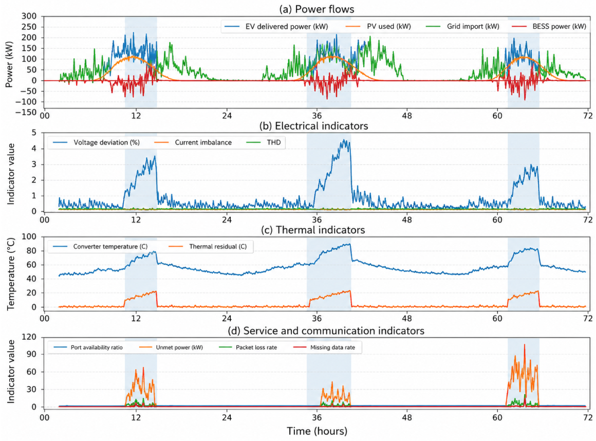
Figure 3 illustrates a representative segment of the generated benchmark and shows how the electrical, renewable-energy, thermal, service, and communication variables evolve jointly. The shaded intervals indicate injected abnormal events. The figure is included to demonstrate the temporal and cross-source structure of the generated data; it is not used as evidence of classifier performance.

The synthetic benchmark is not intended to reproduce one specific public EVCS dataset. Instead, it provides a complete and labeled multi-source environment for controlled evaluation. Public EV and charging datasets support individual components of this problem, including charging-session modeling, charging-profile prediction, battery-health assessment, cyber-security scenarios, and power-quality analysis  [13,18,19,20,21,22,23,28,31]. However, they do not generally provide synchronized PV generation, BESS operation, electrical measurements, thermal indicators, port/session states, communication/data-quality variables, grid-side disturbances, and labeled maintenance faults in one unified schema. The compatibility analysis in Table 1 further shows that existing real-world resources can support component-level calibration or future battery-safety extensions, but not a direct external evaluation of the complete station-level fault-label space considered here.

An extended-horizon benchmark was also generated for longer-term event-level evaluation. This benchmark covers 180 days at the same 5-min sampling resolution and includes weekday/weekend demand variation, weather diversity, seasonal irradiance variation, gradual demand evolution, and drift/ageing proxies. The drift proxies affect thermal residuals, current distortion, current imbalance, communication/data quality, and port/session reliability. The extended benchmark is not a calibrated ageing model; it is used to test whether the framework remains stable when the operating horizon and number of fault events are increased.

To make the benchmark scale, class imbalance, and chronological evaluation protocol explicit,

Table 4. Summary of nominal and extended-horizon benchmark statistics.

Quantity	Value
Nominal 24-day benchmark
Simulation horizon	24 days
Sampling interval	5 min
Raw time samples	6912
Window length/stride	60 min/15 min
Total windows after windowing	2300
Windows used after boundary-buffer exclusion	2277
Training windows	1375
Validation windows	449
Testing windows	453
Boundary-buffer excluded windows	23
Healthy windows	1697
Fault/anomaly windows	603
Injected fault/anomaly events	51
Test fault/anomaly events	16
Full multi-source features	176
Nominal class distribution after windowing before boundary-buffer exclusion
Healthy operation	1697 windows (73.78%)
Converter/open-circuit fault	147 windows (6.39%)
Sensor/measurement fault	89 windows (3.87%)
Thermal/cooling anomaly	140 windows (6.09%)
Port/session failure	76 windows (3.30%)
Communication/data anomaly	73 windows (3.17%)
Grid-side disturbance	78 windows (3.39%)
Extended-horizon benchmark
Simulation horizon	180 days
Raw time samples	51,840
Window length/stride	60 min/15 min
Total windows after windowing	17,276
Injected fault/anomaly events	268
Held-out test fault/anomaly events	81
Minimum minority-class fault windows	442
Long-term variability	Weekday/weekend demand, weather regimes, seasonal irradiance, demand evolution, ageing/drift proxies

summarizes the main nominal and extended-horizon dataset statistics used in the experiments.

3.3.1. Benchmark Design Rationale

To improve reproducibility and clarify the scope of the reported classification performance, the benchmark configuration was selected to represent a controlled station-level EVCS operating scenario rather than a universal model of all charging infrastructures. The objective of the benchmark is to evaluate whether abnormal operational states can be detected from aggregated electrical, thermal, session, grid, and communication variables under realistic monitoring resolutions. Therefore, the benchmark emphasizes persistent station-level abnormal behavior, maintenance-oriented decision support, and interpretable fault–response relationships.

Table 5. Benchmark design rationale and scope limitations.

Benchmark Element	Current Value	Why It Is Reasonable	Sensitivity or Limitation
EVCS aggregate charging rating	320 kW	Represents an 8-port station with moderate aggregate fast-charging capability and sufficient load diversity for operational analysis.	Not intended to represent ultra-fast highway charging hubs or megawatt-scale charging depots.
Number of charging ports	8	Allows port-level availability, session interruption, and service-impact behavior to be evaluated without overcomplicating the benchmark.	Smaller stations may show different availability and queueing impacts.
PV capacity	180 kW	Enables renewable contribution and irradiance-driven variability without assuming full PV autonomy.	Local irradiance, shading, orientation, and site constraints are not optimized in detail.
BESS capacity	350 kWh	Allows peak support, PV buffering, and fault-aware operational response to be represented.	The BESS is not economically optimized, and detailed degradation modeling is outside the study scope.
Sampling interval	5 min	Suitable for station-level monitoring, OCPP/backend data collection, and operational decision support.	Not suitable for fast converter transient diagnosis or protection-level fault detection.
Window length	60 min	Captures persistent abnormal EVCS behavior and reduces sensitivity to isolated measurement fluctuations.	May delay the detection of very fast faults or short-duration protection events.

summarizes the rationale behind the main benchmark settings and the associated limitations.

In addition to the numerical benchmark settings, the injected fault families were selected to preserve a clear relationship between the assumed physical mechanism, the affected variables, and the expected operational response. This relationship is important because the proposed model is intended for maintenance-oriented decision support rather than purely abstract pattern recognition.

Table 6. Fault/anomaly realism and expected operator response.

Fault/Anomaly Class	Physical or Operational Mechanism	Main Affected Variables	Expected Operator Response
Converter/open-circuit	Switch/module abnormality, converter imbalance, or partial converter degradation.	THD, current imbalance, delivered power, converter temperature, DC-bus deviation.	Derate charger, isolate affected converter, inspect power module.
Sensor/measurement	Bias, drift, stale readings, missing values, or measurement-channel degradation.	Sensor residuals, measured/expected mismatch, missing-data rate, data-quality indicators.	Validate sensor, recalibrate, replace transducer, check acquisition chain.
Thermal/cooling	Fan degradation, blocked airflow, cooling-path restriction, or elevated thermal stress.	Temperature residual, thermal slope, cooling margin, derating risk.	Inspect cooling path, clean fan/filter, derate temporarily.
Port/session	Connector, handshake, cable, lock, or port-controller issue.	Failed sessions, interrupted sessions, port availability, delivered session energy.	Isolate port, reroute users, inspect connector and port controller.
Communication/data	OCPP, backend, network, timestamp, or data-quality anomaly.	Packet loss, stale status, missing data, backend delay, inconsistent station state.	Remote reset, network check, backend validation, communication diagnostics.
Grid-side disturbance	Voltage deviation, transformer stress, upstream disturbance, or local grid constraint.	PCC voltage, grid import, BESS response, power-quality indicators.	Reduce load, use BESS support, defer charging, notify grid/operator.

summarizes the physical interpretation of each fault or disturbance family used in the benchmark.

Table 6 should be interpreted as a mechanism–evidence–response mapping for the controlled benchmark. The second column identifies the physical or operational mechanism that motivates each fault/anomaly class, the third column lists the monitored variables expected to change under that mechanism, and the fourth column indicates the corresponding operator action that would be reasonable under a decision-support workflow. For example, a converter/open-circuit event is represented through electrical distortion, current imbalance, reduced delivered power, converter-temperature increase, and DC-bus deviation because these symptoms are consistent with converter imbalance or partial module degradation. A sensor/measurement event is instead represented by bias, drift, missing values, and measured-versus-expected inconsistency, which motivates sensor validation, recalibration, or replacement. Thermal/cooling events are mapped to temperature residuals and derating risk, while port/session events are mapped to failed or interrupted sessions, reduced port availability, and lower delivered session energy. Communication/data events are represented through packet loss, stale status, missing data, backend delay, and inconsistent station state, whereas grid-side disturbances are represented through PCC-voltage deviation, transformer loading, grid import, BESS response, and power-quality indicators. Thus, Table 6 does not define a field-validated maintenance rule. Rather, it documents the engineering rationale linking each injected benchmark fault to observable multi-source evidence and to the type of inspection or response that the proposed decision-support layer is designed to inform.

These tables also define the interpretation boundary of the reported accuracy and macro-F1 values. The reported performance reflects classification under the controlled benchmark assumptions, selected sampling interval, window length, and injected fault mechanisms. Therefore, the results should be interpreted as evidence of strong benchmark-level separability and maintenance-oriented decision-support potential, rather than as a claim of universal field performance across all EVCS designs, protection systems, and site-specific operating conditions.

To reduce temporal leakage, the benchmark was partitioned chronologically using event-level separation and boundary-buffer exclusion. Injected fault/anomaly events were assigned within only one of the training, validation, or test segments, and the event log was checked to confirm that no injected event crossed a partition boundary. Windows that directly crossed a split boundary were excluded. In the nominal configuration, an additional 60-min exclusion margin, equal to one analysis window, was applied around the train–validation and validation–test transitions to reduce dependence between highly adjacent overlapping windows. This procedure excluded 23 of the 2300 generated windows (1.00%), leaving 1375 training, 449 validation, and 453 test windows. Relative to a split with no additional temporal margin, the nominal buffer removed 4 training, 8 validation, and 4 test windows, corresponding to reductions of 0.29%, 1.75%, and 0.88%, respectively. All preprocessing, calibration, and threshold-selection operations were fitted using only the training and validation partitions and then applied unchanged to the held-out test set. The sensitivity of the headline LightGBM result to alternative boundary-buffer widths is evaluated in Section 4.1.

3.3.2. Synthetic-Data Fidelity and Representativeness

The fidelity of the synthetic benchmark was assessed at four complementary levels: system structure, signal relationships, fault mechanisms, and operational variability. The benchmark was not designed to reproduce the exact statistical distribution of one commercial EVCS site. Instead, it was designed to preserve the physical direction, temporal persistence, and cross-source consequences expected from major station-level operating and fault conditions. Table 7 summarizes the corresponding representativeness measures, supporting evaluations, and remaining limitations.

At the system-structure level, the benchmark represents an eight-port, renewable-powered EVCS with coupled charging demand, PV generation, BESS dispatch, grid import, auxiliary demand, electrical measurements, thermal response, port status, and communication/data-quality indicators. The station-level power balance and BESS state-of-charge constraints enforce consistency among local generation, storage, charging load, and grid exchange. This provides greater physical coherence than independently sampling each monitored variable.

At the signal-relationship level, healthy operation preserves interpretable dependencies among load, voltage, current, harmonic distortion, converter temperature, active ports, grid import, and BESS response. For example, charging current is derived from delivered power and voltage, converter temperature responds dynamically to ambient conditions and loading, and grid import reflects the residual demand after PV use and BESS support. These relationships reproduce expected qualitative behavior, although their exact distributions and coefficients are not calibrated to one charger manufacturer or operating site.

At the fault-mechanism level, the six injected fault families were selected from major EVCS failure sources reported in the literature. Each event modifies a physically related subset of variables rather than assigning an arbitrary class label. Converter faults increase distortion, imbalance, thermal stress, and power-delivery loss; sensor faults introduce bias, drift, residual inconsistency, and missing measurements; cooling anomalies alter temperature and thermal residuals; port/session faults reduce service availability and delivered energy; communication faults increase packet loss, stale values, and state inconsistency; and grid disturbances affect voltage, transformer loading, grid import, and BESS response. Table 5 and Table 6 summarize the assumed mechanisms and observable signatures.

Operational representativeness was increased through several forms of variability. The nominal benchmark includes daily charging-demand peaks, stochastic port occupancy, day-to-day irradiance variation, short-term cloud fluctuations, ambient-temperature variation, and variable event durations. Additional hardness experiments introduce reduced fault amplitudes, overlapping signatures, incipient drifts, nonstationary conditions, mixed faults, and measurement perturbations. The 180-day benchmark further incorporates weekday/weekend behavior, weather regimes, seasonal irradiance, gradual demand evolution, and ageing/drift proxies. Repeated-seed experiments evaluate sensitivity to alternative stochastic realizations.

These measures improve controlled-benchmark realism, but they do not establish statistical equivalence to deployed EVCS fleets. The benchmark does not reproduce vendor-specific converter controls, protection logic, charger firmware, site-specific queuing behavior, detailed thermal-fluid dynamics, real fault prevalence, maintenance interventions, or dependencies between weather, usage, degradation, and failure occurrence. Event durations, amplitudes, frequencies, and response assumptions are therefore stress-test parameters rather than empirically estimated field-failure distributions. Accordingly, the benchmark supports reproducible comparison, ablation, and sensitivity analysis, but it cannot substitute for external validation using synchronized charger telemetry, controller logs, OCPP events, protection records, and maintenance-confirmed fault labels.

Table 7. Fidelity dimensions, representativeness measures, and limitations of the controlled EVCS benchmark.

Fidelity Dimension	Representation in the Benchmark	Evidence or Evaluation	Remaining Limitation
System structure	Coupled EV charging load, PV generation, BESS dispatch, grid import, auxiliary load, electrical measurements, thermal response, port states, and communication/data-quality indicators	Power-balance constraint, BESS state-of-charge update, station configuration in Table 3	Not calibrated to one manufacturer, charger topology, or site architecture
Signal relationships	Load-dependent current, voltage, harmonic distortion, converter temperature, grid import, transformer loading, and port/session behavior	Physically interpretable generation equations and cross-source engineered features	Simplified electrical, thermal, queueing, and energy-management models
Fault mechanisms	Six fault families modify source-relevant variables with persistent, class-specific signatures	Mechanism and response mapping in Table 6 and Table 8	Fault amplitudes, durations, prevalence, and co-occurrence are not estimated from field-failure statistics
Short-term variability	Daily demand peaks, stochastic active ports, irradiance fluctuations, cloud variability, ambient-temperature variation, and variable event duration	Nominal 24-day benchmark and five stochastic realizations	Limited representation of rare operational regimes and site-specific user behavior
Hard and ambiguous cases	Reduced-amplitude, overlapping, incipient, mixed, nonstationary, and noise-perturbed faults	Hardness, mixed-fault, open-set, and feature-noise experiments	Cannot guarantee coverage of all field ambiguity or unseen fault combinations
Long-term variability	Weekday/weekend demand, weather regimes, seasonal irradiance, gradual demand evolution, and ageing/drift proxies	Extended 180-day benchmark with 268 injected events and 81 held-out test events	Ageing and drift are proxy models rather than measurements from long-term charger degradation
Operational response	Fault-specific maintenance and DER-aware response scenarios with effectiveness and delay sensitivity	Operational-response, latency, risk-weight, and policy sensitivity analyses	Response effectiveness, economic costs, and intervention outcomes are not field calibrated

Table 7. Fidelity dimensions, representativeness measures, and limitations of the controlled EVCS benchmark.

Fidelity Dimension	Representation in the Benchmark	Evidence or Evaluation	Remaining Limitation
System structure	Coupled EV charging load, PV generation, BESS dispatch, grid import, auxiliary load, electrical measurements, thermal response, port states, and communication/data-quality indicators	Power-balance constraint, BESS state-of-charge update, station configuration in Table 3	Not calibrated to one manufacturer, charger topology, or site architecture
Signal relationships	Load-dependent current, voltage, harmonic distortion, converter temperature, grid import, transformer loading, and port/session behavior	Physically interpretable generation equations and cross-source engineered features	Simplified electrical, thermal, queueing, and energy-management models
Fault mechanisms	Six fault families modify source-relevant variables with persistent, class-specific signatures	Mechanism and response mapping in Table 6 and Table 8	Fault amplitudes, durations, prevalence, and co-occurrence are not estimated from field-failure statistics
Short-term variability	Daily demand peaks, stochastic active ports, irradiance fluctuations, cloud variability, ambient-temperature variation, and variable event duration	Nominal 24-day benchmark and five stochastic realizations	Limited representation of rare operational regimes and site-specific user behavior
Hard and ambiguous cases	Reduced-amplitude, overlapping, incipient, mixed, nonstationary, and noise-perturbed faults	Hardness, mixed-fault, open-set, and feature-noise experiments	Cannot guarantee coverage of all field ambiguity or unseen fault combinations
Long-term variability	Weekday/weekend demand, weather regimes, seasonal irradiance, gradual demand evolution, and ageing/drift proxies	Extended 180-day benchmark with 268 injected events and 81 held-out test events	Ageing and drift are proxy models rather than measurements from long-term charger degradation
Operational response	Fault-specific maintenance and DER-aware response scenarios with effectiveness and delay sensitivity	Operational-response, latency, risk-weight, and policy sensitivity analyses	Response effectiveness, economic costs, and intervention outcomes are not field calibrated

Table 8. Injected fault/anomaly classes and their main operating signatures.

Class	Main Injected Operating Signature
Healthy operation	Normal PV generation, BESS operation, charging demand, electrical measurements, thermal response, port status, and communication indicators.
Converter/open-circuit fault	Increased current distortion and imbalance, reduced delivered charging power, increased unmet power, elevated converter temperature, and increased power-balance residual.
Sensor/measurement fault	Current or voltage bias, measurement drift, inconsistency between measured and expected values, residual error increase, and occasional missing-data behavior.
Thermal/cooling anomaly	Abnormal converter-temperature rise, increased thermal residual, and mild harmonic increase under otherwise comparable loading conditions.
Port/session failure	Reduced port availability, increased failed or interrupted sessions, reduced delivered charging power, and increased unmet charging demand.
Communication/data anomaly	Increased packet loss, missing-data rate, stale measurements, status inconsistency, and occasional spoofed or stale measurement behavior.
Grid-side disturbance	Voltage deviation, increased grid import, increased transformer loading, BESS response, and moderate current-distortion increase.

Table 8. Injected fault/anomaly classes and their main operating signatures.

Class	Main Injected Operating Signature
Healthy operation	Normal PV generation, BESS operation, charging demand, electrical measurements, thermal response, port status, and communication indicators.
Converter/open-circuit fault	Increased current distortion and imbalance, reduced delivered charging power, increased unmet power, elevated converter temperature, and increased power-balance residual.
Sensor/measurement fault	Current or voltage bias, measurement drift, inconsistency between measured and expected values, residual error increase, and occasional missing-data behavior.
Thermal/cooling anomaly	Abnormal converter-temperature rise, increased thermal residual, and mild harmonic increase under otherwise comparable loading conditions.
Port/session failure	Reduced port availability, increased failed or interrupted sessions, reduced delivered charging power, and increased unmet charging demand.
Communication/data anomaly	Increased packet loss, missing-data rate, stale measurements, status inconsistency, and occasional spoofed or stale measurement behavior.
Grid-side disturbance	Voltage deviation, increased grid import, increased transformer loading, BESS response, and moderate current-distortion increase.

3.4. Fault and Anomaly Injection

Six fault/anomaly categories were injected into the healthy EVCS time series: converter/open-circuit faults, sensor/measurement faults, thermal/cooling anomalies, port/session failures, communication/data anomalies, and grid-side disturbances. These categories were selected because they represent major EVCS fault sources reported in the literature, including power-electronic faults, measurement faults, thermal stress, charging-service failures, communication/data-quality problems, and grid-interactive disturbances [5,6,8,10,12,24].

Fault events were injected into the chronological training, validation, and testing segments to ensure that all classes were represented in each stage of the evaluation. Event durations ranged from 1 to 4 h, with spacing between events to reduce overlap. The injected signatures were designed to be physically interpretable and diagnostically meaningful, but they are not intended to represent calibrated field-failure distributions or real-world event frequencies.

To examine the effect of fault separability, additional benchmark variants were generated. These variants included reduced-amplitude faults, severity-scaled faults, overlapping class signatures, incipient drifting faults, nonstationary operating conditions, and mixed or compound faults involving more than one fault source. These variants were used for robustness and open-set evaluation rather than replacing the nominal benchmark. The main injected operating signatures associated with each healthy or faulty EVCS class are summarized in Table 8.

3.5. Multi-Source Monitoring Representation

To represent the heterogeneous monitoring environment of a renewable-powered EVCS, the raw station measurements are grouped according to their physical or operational source. This grouping enables the diagnostic models to use information from multiple subsystems while also allowing the explainability layer to identify which source group contributes most strongly to each detected fault or anomaly. At each time step t, the monitored EVCS state is represented as

$$\mathbf{x}\left(t\right)=\left[{\mathbf{x}}_{\mathrm{elec}}\left(t\right),{\mathbf{x}}_{\mathrm{th}}\left(t\right),{\mathbf{x}}_{\mathrm{sess}}\left(t\right),{\mathbf{x}}_{\mathrm{grid}}\left(t\right),{\mathbf{x}}_{\mathrm{comm}}\left(t\right)\right].$$

(3)

where ${\mathbf{x}}_{\mathrm{elec}}\left(t\right)$ contains electrical variables, ${\mathbf{x}}_{\mathrm{th}}\left(t\right)$ contains thermal variables, ${\mathbf{x}}_{\mathrm{sess}}\left(t\right)$ contains session and port variables, ${\mathbf{x}}_{\mathrm{grid}}\left(t\right)$ contains grid/PV/BESS variables, and ${\mathbf{x}}_{\mathrm{comm}}\left(t\right)$ contains communication and data-quality variables.

The electrical source group includes voltage, current, delivered power, current imbalance, total harmonic distortion, and power-balance residual. The thermal group includes ambient temperature, converter temperature, and load-normalized thermal residual. The session/port group includes active ports, requested power, delivered power, unmet power, port availability, failed-session flags, interrupted-session flags, and session-duration proxies. The grid/PV/BESS group includes PV availability, PV use, grid import, BESS power, BESS SOC, voltage deviation, transformer loading, and PV utilization. The communication/data group includes packet-loss rate, missing-data rate, status inconsistency, stale-measurement flags, and data-quality risk indicators.

This source grouping is central to the proposed framework because different EVCS faults appear through different evidence channels. Converter faults are expected to affect electrical and thermal indicators, sensor faults affect residual and measurement-consistency indicators, thermal anomalies affect temperature and load-normalized residuals, port/session failures affect charging-service indicators, communication/data anomalies affect packet-loss and status-consistency indicators, and grid-side disturbances affect voltage, grid import, BESS response, and transformer-loading variables.

3.6. Windowing, Preprocessing, and Feature Extraction

Because EVCS operation is time-dependent, the raw time series was converted into sliding windows. The nominal window length was set to 12 samples, corresponding to 1 h at a 5-min sampling interval. The stride was set to 3 samples, corresponding to 15 min. The kth observation window is defined as

$${\mathbf{X}}_k=\left[\mathbf{x}(t_k-W+1),\mathbf{x}(t_k-W+2),\dots ,\mathbf{x}\left(t_k\right)\right],$$

(4)

where W is the window length.

A window was assigned to a fault class if at least 30% of its samples belonged to that fault class. Otherwise, the window was labeled as healthy. This rule reduces boundary contamination while allowing early portions of fault events to be represented. Preprocessing included time alignment, missing-value treatment, and median imputation. Feature scaling was applied on a model-specific basis rather than uniformly to all classifiers. During model development, median-imputation and z-score standardization parameters for scale-sensitive models were estimated using the training partition and applied unchanged to the validation partition. After the model configurations and decision rules had been fixed, the preprocessing pipeline and final supervised model were refitted using the combined training and validation partitions and applied once to the chronologically held-out test partition. No preprocessing parameter was estimated from the held-out test data.

For scale-sensitive models, each continuous feature $x_j$ was standardized using the z-score transformation

$$z_j={\displaystyle \frac{x_j-{\mu }_j}{{\sigma }_j}},$$

(5)

where $m{u}_j$ and ${\sigma }_j$ are the mean and standard deviation of feature j, respectively, estimated from the relevant model-fitting partition. Z-score standardization was implemented using the StandardScaler transformation in scikit-learn [37]. It was selected because the engineered feature set contains heterogeneous units and numerical ranges, including voltage, current, temperature, energy, packet-loss rates, and binary indicators; without scaling, variables with larger numerical magnitudes could disproportionately influence linear, kernel-based, and neural-network models. Tree-based classifiers, including Random Forest, Extra Trees, HistGradientBoosting, Balanced Random Forest, XGBoost, LightGBM, and CatBoost, were trained without predictor standardization because their split-based operation does not require features to share a common numerical scale.

For each monitored variable, statistical and temporal features were extracted over the window, including mean, standard deviation, minimum, maximum, final value, and least-squares slope. Additional engineered features included load-normalized temperature, maximum temperature rise above ambient, PV utilization, unmet energy, grid-import energy, BESS throughput, voltage-violation proxy, transformer-loading proxy, and data-quality risk. The resulting feature vector for window k is denoted by ${\mathbf{z}}_k$.

For power-quality monitoring, total harmonic distortion is represented as

$$TH{D}_I={\displaystyle \frac{\sqrt{{\sum }_{h=2}^H{I}_h^2}}{I_1}},$$

(6)

where $I_1$ is the fundamental current component and $I_h$ is the hth harmonic current component. For thermal monitoring, the thermal residual is defined as

$$r_T\left(t\right)=T_{\mathrm{meas}}\left(t\right)-\widehat{T}\left(t\right),$$

(7)

where $T_{\mathrm{meas}}\left(t\right)$ is the measured converter temperature and $\widehat{T}\left(t\right)$ is the expected temperature under the corresponding load, ambient, and operating conditions.

3.7. Chronological Data Splitting and Evaluation Tasks

The benchmark was split chronologically to reduce leakage between adjacent windows. The first 60% of the simulation horizon was used for training, the next 20% for validation, and the final 20% for testing. Fault events were injected independently within the training, validation, and testing segments, with a one-window boundary buffer around the split transitions. Therefore, no individual fault event was shared across model-fitting and held-out evaluation segments.

The evaluation protocol includes five tasks. First, closed-set fault classification evaluates whether known EVCS fault categories can be identified when all classes are represented during training. Second, feature-source ablation evaluates the contribution of electrical, thermal, session/port, grid/PV/BESS, and communication/data sources. Third, open-set and anomaly-detection experiments evaluate whether unknown or anomalous events can be flagged. Fourth, explainability analysis evaluates whether the dominant feature-source groups are consistent with expected fault origins. Fifth, operational-impact assessment evaluates how earlier diagnostic warnings could affect service and grid-interactive indicators under explicit response assumptions.

3.8. Diagnostic Models

The diagnostic layer combines closed-set fault classification for known EVCS operating and fault classes with anomaly/open-set detection for unknown or anomalous operating conditions. This hybrid structure is used because practical EVCS monitoring must identify known fault categories when labeled examples are available while also flagging abnormal behavior that may not correspond to any class observed during training.

For known operating and fault classes, supervised classifiers were trained using the extracted feature vectors. The classifier output for a window k is

$${\mathbf{p}}_k=\left[p(y=1|{\mathbf{z}}_k),p(y=2|{\mathbf{z}}_k),\dots ,p(y=C|{\mathbf{z}}_k)\right],$$

(8)

where C is the number of known classes and ${\mathbf{z}}_k$ is the feature vector for window k.

The primary diagnostic models included Logistic Regression, Random Forest, and Extra Trees. Logistic Regression provides a linear baseline, while Random Forest and Extra Trees provide nonlinear ensemble baselines suitable for heterogeneous tabular features. To ensure that the results were not dependent on one classifier family, additional imbalance-aware tabular baselines were evaluated, including gradient-boosting and class-weighted ensemble models. Raw time-series baselines were also evaluated using sequence-based input representations to compare engineered window features against direct temporal models. Class imbalance was handled using class weights or balanced sample weights where supported by the model. The supervised-model configurations were fixed before the held-out test evaluation; no grid search, random search, or test-driven hyperparameter optimization was performed. The configurations were chosen as standard reproducible settings for the respective classifier families. After the configurations had been fixed, each final supervised model was fitted using the combined training and validation partitions, comprising 1824 windows, and evaluated once on the chronologically held-out test partition of 453 windows. The candidate classifier families and their configurations were specified before held-out evaluation. All candidate-model results are reported, and no model was re-tuned, removed, or replaced based on test performance. Among these pre-specified candidates, LightGBM achieved the highest observed held-out macro-F1.

Table 9. Principal configurations of the supervised tabular classifiers. Configurations were fixed before held-out test evaluation, and parameters not listed were retained at their library defaults.

Classifier	Principal Configuration	Imbalance Treatment
Logistic Regression	median imputation; z-score standardization; maximum iterations = 1500; fixed random seed	balanced class weights
Random Forest	median imputation; 120 trees; unrestricted maximum depth; minimum samples per leaf = 2; fixed random seed	balanced-subsample class weighting
Extra Trees	median imputation; 120 trees; unrestricted maximum depth; minimum samples per leaf = 2; fixed random seed	balanced class weighting
HistGradientBoosting	median imputation; 180 boosting iterations; learning rate = 0.06; $L_2$ regularization = 0.01; fixed random seed	class-balanced sample weights
Balanced Random Forest	median imputation; 180 trees; minimum samples per leaf = 2; fixed random seed	class-balanced bootstrap sampling
XGBoost	median imputation; 220 trees; maximum depth = 4; learning rate = 0.05; row subsampling = 0.90; feature subsampling = 0.90; multiclass probabilistic objective; fixed random seed	class-balanced sample weights
LightGBM	median imputation; 240 trees; learning rate = 0.05; number of leaves = 31; fixed random seed	balanced class weighting
CatBoost	median imputation; 260 boosting iterations; tree depth = 5; learning rate = 0.05; multiclass loss; fixed random seed	automatic balanced class weighting

summarizes the principal supervised-model configurations.

For comparison with the engineered-feature models, raw multi-source sequence baselines were also evaluated. For each retained window, the raw-sequence input was represented as a $12\times 28$ tensor, corresponding to 12 time steps over the 1-h analysis window and 28 monitored raw variables from the electrical, thermal, session/port, grid/PV/BESS, and communication/data groups. Sequence features were standardized channel-wise using the combined training–validation partition and then applied unchanged to the held-out test partition. The 1D-CNN baseline consisted of two temporal convolutional layers: a Conv1D layer with 48 filters, kernel size 3, padding 1, and ReLU activation, followed by a Conv1D layer with 64 filters, kernel size 3, padding 2, dilation 2, and ReLU activation. The convolutional features were aggregated using adaptive average pooling over the time dimension, followed by flattening, dropout with probability 0.10, and a linear output layer producing seven class logits. Training used weighted cross-entropy loss with inverse-frequency class weights normalized by their mean, the Adam optimizer with learning rate ${10}^{-3}$ and weight decay ${10}^{-4}$, mini-batches of 128 windows, and 10 training epochs. The 1D-CNN configuration was fixed before held-out evaluation and was fitted on the same combined training–validation partition used for the final supervised-model comparison. No validation-based early stopping or test-driven tuning was used for this raw-sequence baseline.

For anomaly and open-set detection, one-class and reconstruction-based models were trained using healthy training windows only. Healthy validation windows were used to select the anomaly threshold, and the test set was used only for final evaluation. For a window k, the anomaly detector produces a score $s_k$, where larger values indicate more abnormal behavior. The nominal threshold is selected from the healthy validation score distribution:

$$\tau =Q_{0.95}\left(s_k\mid y_k=0,k\in \mathcal{V}\right),$$

(9)

where $\mathcal{V}$ denotes the validation set and $Q_{0.95}$ is the 95th percentile. A window is flagged as anomalous if

$$s_k>\tau .$$

(10)

A leave-one-class-out open-set protocol was used to evaluate unknown-fault behavior. In each fold, one fault category was excluded from the model-fitting procedure and treated as unknown during testing. The procedure was repeated across all six fault categories. Mixed-fault cases and distribution-shifted normal cases were also evaluated to distinguish truly abnormal unseen events from unseen but non-fault operating variability. For reconstruction-based anomaly detection, the reconstruction error of a window is defined as

$$e_k={\displaystyle \frac{1}{Wm}}{∥{\mathbf{X}}_k-{\widehat{\mathbf{X}}}_k∥}_2^2,$$

(11)

where m is the number of monitored variables and ${\widehat{\mathbf{X}}}_k$ is the reconstructed window.

3.9. Explainability and Risk Mapping

The explainability and risk-mapping layer is designed to support maintenance interpretation rather than only model transparency. For tree-based supervised models, feature importance was computed and then grouped by monitoring source. The grouped importance of source g is

$$I_g=\sum _{j\in {\mathcal{G}}_g}{I}_j,$$

(12)

where $G_g$ is the set of features belonging to source group g, and $I_j$ is the importance assigned to feature j by the corresponding explanation method. After summing the feature-level values within each source group, the five source-group totals were divided by their overall sum to obtain relative source contributions that sum to one. This normalization was applied separately for each explanation method because native impurity importance, permutation importance, and TreeSHAP produce values on different numerical scales.

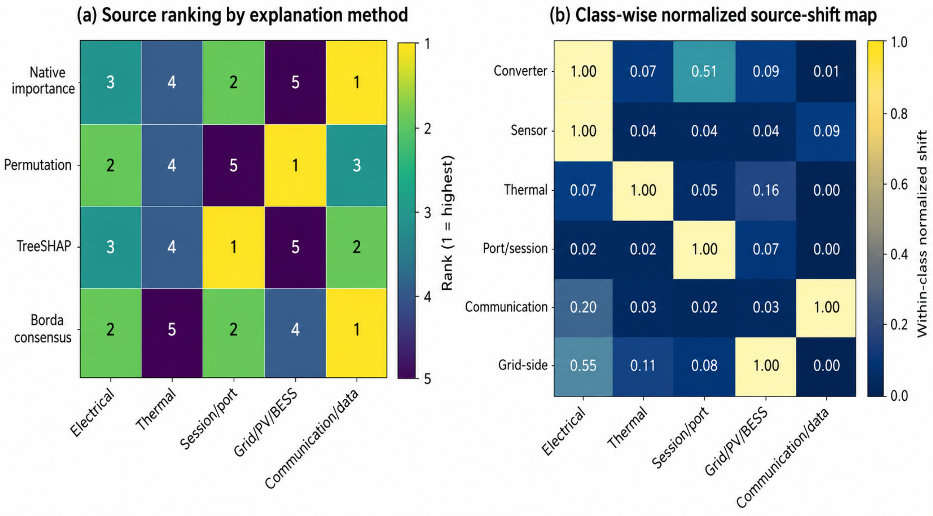
A class-wise source-shift map was also computed. For each fault class, the median feature profile in the test set was compared with the median healthy training profile using a robust scale based on the healthy interquartile range and global feature variability. For visualization, the five source-strength values within each fault-class row were divided by the maximum source-strength value in that row. Consequently, the dominant source for each class was displayed as 1, while the remaining sources were represented relative to that class-specific maximum. This row-wise normalization was used only to improve comparison within each fault class; the unnormalized robust source-shift values were retained in the numerical outputs and used for the underlying analysis. For example, converter faults are expected to be associated mainly with electrical and thermal evidence, port/session failures with session and port indicators, and communication/data anomalies with packet-loss, missing-data, stale-measurement, and status-inconsistency features. The explainability output is not treated as causal proof; instead, it provides source-aware diagnostic evidence that can help operators interpret why a window was flagged and which subsystem should be inspected first.

Because different explanation methods quantify different notions of feature relevance, a rank-aggregation procedure was introduced to avoid treating any single global importance method as the definitive source of causal evidence. For each explanation method (m), the five monitoring-source groups were ordered from highest to lowest importance. A Borda consensus score was calculated for source group g as

$$B_g={\displaystyle \sum _{m=1}^M}\left(G-r_{g,m}\right),B_g^{\mathrm{norm}}={\displaystyle \frac{B_g}{M(G-1)}},$$

(13)

where $M=3$ is the number of explanation methods, $G=5$ is the number of source groups, and $r_{g,m}$ is the rank of source g by method m. The normalized consensus score is $B_g/\left[M(G-1)\right]$. This rank-based procedure was selected because native impurity importance, permutation importance, and TreeSHAP quantify feature relevance differently and produce values on different numerical scales.

The consensus ranking is used as a model-level robustness indicator and not as a stand-alone causal fault-source diagnosis. For an individual alarm, the predicted fault class and the corresponding class-wise source-shift map are used to identify the dominant and secondary inspection sources. Where the explanation evidence remains inconsistent, the output is treated as a multi-source or ambiguous alert requiring operator review rather than an autonomous maintenance action.

The diagnostic outputs are then translated into maintenance-oriented decision-support states through a heuristic risk score. For each window k, the risk score is defined as

$$R_k=0.35S_k+0.20C_k+0.20P_k+0.15O_k+0.10A_k,$$

(14)

where $S_k$ is the class-dependent severity component, $C_k$ is the diagnostic confidence component, $P_k$ is the persistence of abnormal behavior across recent windows, $O_k$ is the operational-impact component, and $A_k$ is the normalized anomaly-score component.

Table 10. Definition of the normalized components used in the maintenance-oriented risk score.

Component	Meaning	Nominal Computation	Range
$S_k$	Class-dependent severity	Assigned from the predicted operating/fault class using the fixed severity map in Table 11.	0–1
$C_k$	Diagnostic confidence	Maximum supervised-classifier posterior probability for the predicted class. If posterior probabilities are unavailable, a fixed confidence value of 0.75 is used.	0–1
$P_k$	Persistence of abnormal behavior	Rolling mean of anomaly flags over the most recent four windows, corresponding to approximately one hour under the 15-min stride.	0–1
$O_k$	Operational-impact component	Weighted combination of normalized unmet charging energy, port unavailability, transformer loading, and data-quality risk, using weights 0.35, 0.25, 0.20, and 0.20, respectively. Each indicator was normalized using limits estimated from the combined training and validation reference distribution and then applied unchanged to the held-out test set.	0–1
$A_k$	Anomaly-strength component	Anomaly score transformed to [0,1] using the 5th and 95th percentiles estimated from the combined training and validation reference distribution. The fitted limits were applied unchanged to the held-out test set, and values outside the reference interval were clipped.	0–1

defines the five normalized components used in the risk score and clarifies how each component is computed in the nominal decision-support configuration. The class-dependent severity component $S_k$ is assigned using the fixed severity mapping summarized in

Table 11. Class-severity mapping used in the nominal risk-score configuration.

Predicted Class	Severity Score	Rationale
Healthy operation	0.00	No maintenance action required under normal monitoring.
Converter/open-circuit fault	0.90	High severity because converter faults can reduce delivered power, increase distortion, and require derating or isolation.
Sensor/measurement fault	0.60	Moderate severity because measurement faults degrade diagnostic and control trust but may not immediately stop charging service.
Thermal/cooling anomaly	0.75	Medium-high severity because abnormal thermal behavior may indicate cooling degradation or component stress.
Port/session failure	0.85	High severity because port/session failures directly reduce service availability and increase unmet charging demand.
Communication/data anomaly	0.55	Moderate severity because communication/data faults reduce monitoring and remote-control reliability but may not always indicate immediate power-delivery failure.
Grid-side disturbance	0.65	Medium-high severity because grid disturbances affect voltage quality, transformer loading, BESS dispatch, and grid-interactive operation.

. Table 10 and Table 11 are original methodological constructs developed for this study and are not reproduced or adapted from a published source. The qualitative rationale is informed by the EVCS fault and maintenance literature reviewed in Section 2, whereas the numerical severity values and component weights are explicit engineering assumptions evaluated through sensitivity analysis.

The severity, diagnostic-confidence, and persistence components are inherently bounded within [0, 1]. The operational-impact and anomaly-strength components were normalized using limits estimated exclusively from the combined training and validation partitions, comprising 1824 reference windows, and the fitted limits were subsequently applied unchanged to the held-out test set. For transformer loading, data-quality risk, and anomaly strength, the lower and upper limits were defined by the 5th and 95th percentiles of the complete reference distribution. For the nonnegative and zero-inflated unmet-energy and port-unavailability indicators, zero was retained as the physical lower bound, while the upper limit was defined by the 95th percentile of the positive reference values. This treatment prevents the normalization interval from becoming degenerate when most reference windows exhibit no service loss. For a raw component u, the normalized value was calculated as

$$\tilde{u}=clip\left({\displaystyle \frac{u-L_u^{\mathrm{ref}}}{U_u^{\mathrm{ref}}-L_u^{\mathrm{ref}}}},0,1\right),$$

(15)

where $L_u^{\mathrm{ref}}$ and $U_u^{\mathrm{ref}}$ denote the fitted lower and upper limits. Values outside the fitted interval were clipped to [0, 1]. This robust percentile-based transformation was selected to reduce sensitivity to isolated extreme fault values while providing bounded and comparable inputs to the risk score.

The coefficients in Equation (14) were not assigned randomly and were not estimated using the held-out test set. Because field maintenance-cost records and operator-calibrated utility functions were unavailable, the nominal coefficient vector was defined a priori using a transparent engineering-priority scheme. Raw priority scores of $q=[7,4,4,3,2]$ were assigned to fault severity, diagnostic confidence, abnormality persistence, operational impact, and anomaly strength, respectively. The normalized coefficient for component (i) was then calculated as $w_i={\displaystyle \frac{q_i}{{\sum }_{j=1}^5{q}_j}},$ which yields ${\mathbf{w}}_0=[0.35,0.20,0.20,0.15,0.10].$ Fault severity received the largest weight because the expected safety and service consequences should dominate maintenance urgency. Diagnostic confidence and persistence received equal intermediate weights so that an intervention requires both credible and sustained evidence rather than a single uncertain or transient alarm. Operational impact received a slightly lower weight because service loss and grid stress partly overlap with the class-severity component. Anomaly strength received the smallest weight because it provides complementary evidence for unusual behavior but is sensitive to threshold selection and may not directly identify the fault source. The resulting score is therefore an interpretable and operator-adjustable decision-support index, not a statistically optimized or field-validated maintenance policy. The dependence of the operational conclusions on this nominal choice was evaluated through alternative weighting schemes and Monte Carlo weight perturbations. The normalized risk-score components are defined in Table 10, while the corresponding class-severity mapping is reported in Table 11.

The continuous risk score is mapped into four health states:

$$H_k=\left\{\begin{array}{cc}\mathrm{Healthy},\hfill & R_k<{\theta }_1,\hfill \\ \mathrm{Warning},\hfill & {\theta }_1\le R_k<{\theta }_2,\hfill \\ \mathrm{Degraded},\hfill & {\theta }_2\le R_k<{\theta }_3,\hfill \\ \mathrm{Critical},\hfill & R_k\ge {\theta }_3.\hfill \end{array}\right.$$

(16)

In the nominal configuration, the health-state thresholds were set to $({\theta }_1,{\theta }_2,{\theta }_3)=(0.25,0.45,0.70)$. Therefore, windows with $R_k<0.25$ were labeled Healthy, windows with $0.25\le R_k<0.45$ were labeled Warning, windows with $0.45\le R_k<0.70$ were labeled Degraded, and windows with $R_k\ge 0.70$ were labeled Critical. Healthy states correspond to normal monitoring. Warning states indicate closer observation or scheduled inspection. Degraded states indicate maintenance planning, charger derating, or targeted inspection depending on the dominant source-level evidence. Critical states indicate immediate intervention, affected-port isolation, or charger shutdown depending on the inferred fault source and safety implications. These states are decision-support flags over time and do not imply that every flagged window corresponds to a separate physical maintenance dispatch. In practice, consecutive warning, degraded, or critical windows would be aggregated before an operator schedules inspection or intervention.

3.10. Operational and DER-Aware Response Assessment

The operational-response layer evaluates how earlier fault detection could affect EVCS service and grid-interactive indicators under explicit response assumptions. The main indicators include port availability, unavailable port hours, failed or interrupted sessions, unmet charging energy, grid import, PV utilization, BESS throughput, transformer-loading exposure, and risk-triggered action windows.

Port availability over an evaluation period is defined as

$$A_{\mathrm{port}}={\displaystyle \frac{T_{\mathrm{available}}}{T_{\mathrm{total}}}},$$

(17)

where $T_{\mathrm{available}}$ is the time during which charging service is available and $T_{\mathrm{total}}$ is the total evaluation time. PV utilization is defined as

$$U_{\mathrm{PV}}={\displaystyle \frac{E_{\mathrm{PV},\mathrm{used}}}{E_{\mathrm{PV},\mathrm{generated}}}},$$

(18)

where $E_{\mathrm{PV},\mathrm{used}}$ is the PV energy used locally for EV charging, BESS charging, or auxiliary loads, and $E_{\mathrm{PV},\mathrm{generated}}$ is the total generated PV energy.

Two service-response policies are compared. The first is a reactive policy, in which fault impacts remain active for the full injected event duration. The second is a fault-aware response policy, in which warning, degraded, or critical decision states enable earlier intervention. Because actual intervention effectiveness is not field-validated in this study, the operational assessment is treated as a scenario-based sensitivity analysis. The nominal response case assumes that, after early detection, the remaining unavailable-port duration and remaining unmet charging energy are partially reduced. These assumptions are not interpreted as measured maintenance savings; they define one operating point within a broader response-sensitivity analysis.

To evaluate the dependence of the operational outcome on intervention assumptions, response effectiveness is swept across a range of unavailable-duration and unmet-energy reduction factors. Additional decision-latency scenarios are evaluated by delaying the effective intervention after detection. A fault-type-specific response model is also considered because converter faults, thermal anomalies, sensor faults, port/session failures, communication/data anomalies, and grid-side disturbances do not have identical remediation dynamics.

The renewable-powered and grid-interactive context is assessed through an additional DER-aware response scenario. In the maintenance-only response, early intervention affects service availability and unmet charging energy, but PV utilization, grid import, and BESS dispatch are kept unchanged. In the DER-aware response, risk-triggered actions may also modify local energy-management behavior through charger derating, BESS support, PV reallocation, grid-peak reduction, and transformer-overload mitigation.

The DER-aware response model is fault-type specific. Converter/open-circuit faults are linked to protective charger derating and limited BESS support. Thermal/cooling anomalies are linked to thermal derating and BESS support during constrained charging. Port/session failures are linked to port rerouting and local PV/BESS support for remaining active ports. Communication/data anomalies are linked mainly to remote reset and data-quality recovery because they do not necessarily require DER redispatch. Grid-side disturbances are linked to BESS-assisted peak shaving and grid-aware charging derating.

The maintenance-only and DER-aware policies represent different operating objectives and should not be interpreted as universally ordered alternatives. Under normal grid conditions, the maintenance-only policy prioritizes rapid restoration of charging service. The DER-aware policy is intended for periods in which a binding thermal, transformer-loading, grid-capacity, demand-charge, or renewable-curtailment constraint justifies temporary charging derating. An operator can select between the two policies using a site-specific cost function

$$J_p=c_{\mathrm{u}}{H}_{\mathrm{u},p}+c_{\mathrm{e}}{E}_{\mathrm{unmet},p}+c_{\mathrm{g}}{E}_{\mathrm{grid},p}+c_{\mathrm{pk}}{P}_{\mathrm{peak},p}+c_{\mathrm{curt}}{E}_{\mathrm{curt},p}+c_{\mathrm{tr}}{H}_{\mathrm{over},p}+c_{\mathrm{b}}{E}_{\mathrm{BESS},p},$$

(19)

where p denotes the candidate policy; $H_{\mathrm{u}}$ is unavailable-port time; $E_{\mathrm{unmet}}$ is unmet charging energy; $E_{\mathrm{grid}}$ is imported grid energy; $P_{\mathrm{peak}}$ is peak grid demand; $E_{\mathrm{curt}}$ is curtailed PV energy; $H_{\mathrm{over}}$ is transformer-overload exposure; and $E_{\mathrm{BESS}}$ is BESS throughput. The coefficients represent operator-specific service-loss costs, energy tariffs, demand charges, renewable-curtailment penalties, transformer-risk costs, and battery-degradation costs. The DER-aware policy is preferable only when the avoided grid, peak-demand, curtailment, and transformer-risk costs exceed the additional service-loss and BESS-cycling costs relative to maintenance-only operation. When continued full-power operation violates a thermal, converter, or grid-security limit, safety constraints take precedence over economic optimization.

3.11. Evaluation Metrics and Implementation

Closed-set classification performance is evaluated using accuracy, macro precision, macro recall, macro-F1, per-class precision, per-class recall, per-class F1-score, and confusion matrices. Macro-F1 is emphasized because the benchmark is class-imbalanced and because diagnostic performance should not be dominated by the healthy class.

Open-set and anomaly-detection performance is evaluated using ROC-AUC, PR-AUC, F1-score, precision, recall, false-alarm rate, and unknown-class recall. Feature-source ablation is evaluated by comparing the full multi-source feature set with reduced feature sets. Explainability is evaluated using grouped feature-source importance and class-wise source-shift maps. Computational feasibility is assessed using training time, inference time per window, and total pipeline runtime. Operational performance is evaluated using port availability, unavailable port hours, failed/interrupted sessions, unmet charging energy, grid import, PV utilization, BESS throughput, transformer-overload exposure, and risk-triggered action windows.

For the supervised comparison, all candidate classifiers used the fixed configurations reported in Table 9, were refitted on the combined training–validation partition, and were evaluated on the same held-out test partition. The simulation and learning pipeline was implemented in Python 3.14.1 and organized to support reproducibility. The pipeline includes modules for synthetic EVCS time-series generation, fault/anomaly injection, sliding-window feature extraction, chronological data splitting, supervised model training and evaluation, anomaly/open-set analysis, source-level explainability, risk-state mapping, and scenario-based operational-response assessment. Fixed random seeds were used for the nominal benchmark, and repeated-seed experiments were performed to assess stochastic stability. To support reproducibility, the repository accompanying this study provides the synthetic data-generation script, fault-injection script, feature-extraction script, model-training and evaluation script, configuration files, fixed random seeds, and scripts used to generate the reported tables and figures.

4. Results and Discussion

This section evaluates the proposed fault-aware decision-support framework using the scenario-controlled EVCS benchmark described in Section 3. The results are organized around five questions: (i) how accurately known EVCS fault classes can be diagnosed, (ii) whether multi-source monitoring improves performance compared with electrical-only monitoring, (iii) whether unknown or compound faults can be detected, (iv) whether the explanations are consistent with the injected fault sources, and (v) how diagnostic outputs affect service-oriented and grid-interactive indicators under explicit response assumptions. Unless otherwise stated, all reported metrics are computed on the chronologically held-out test set.

4.1. Closed-Set Diagnosis of Known EVCS Fault Classes

The first experiment evaluates closed-set classification, where all operating and fault classes are represented during model fitting. All classifiers used the fixed configurations reported in Table 9, the same combined training–validation partition, and the same chronologically held-out test partition.

Table 12. Comparison with stronger imbalance-aware tabular supervised baselines.

Model	Accuracy	Macro Precision	Macro Recall	Macro-F1	Inference (ms/Window)
LightGBM + class weights	0.9845	0.9720	0.9878	0.9792	0.0354
HistGradientBoosting + balanced weights	0.9823	0.9779	0.9769	0.9764	0.0370
XGBoost + class weights	0.9757	0.9618	0.9757	0.9674	0.0204
RandomForest	0.9735	0.9591	0.9693	0.9626	0.1071
ExtraTrees	0.9647	0.9388	0.9723	0.9542	0.0744
CatBoost + class weights	0.9536	0.9243	0.9731	0.9456	0.0338
BalancedRandomForest	0.9360	0.8891	0.9652	0.9238	0.1015
LogisticRegression	0.9227	0.9287	0.8778	0.8867	0.0078

summarizes their performance. The best closed-set result was obtained by LightGBM with class weights, achieving 98.45% accuracy and a macro-F1 score of 0.9792. HistGradientBoosting with balanced sample weights achieved a closely comparable result, with 98.23% accuracy and 0.9764 macro-F1, while XGBoost achieved 97.57% accuracy and 0.9674 macro-F1. These results show that the engineered multi-source representation produced consistently strong held-out performance across several imbalance-aware tabular models under the controlled benchmark. The Random Forest model achieved 97.35% accuracy and a macro-F1 score of 0.9626. Although it was not the strongest closed-set classifier, it was retained for detailed confusion-matrix analysis, explainability, and maintenance-decision experiments because it provides a strong balance between diagnostic performance, interpretability, and computational efficiency.

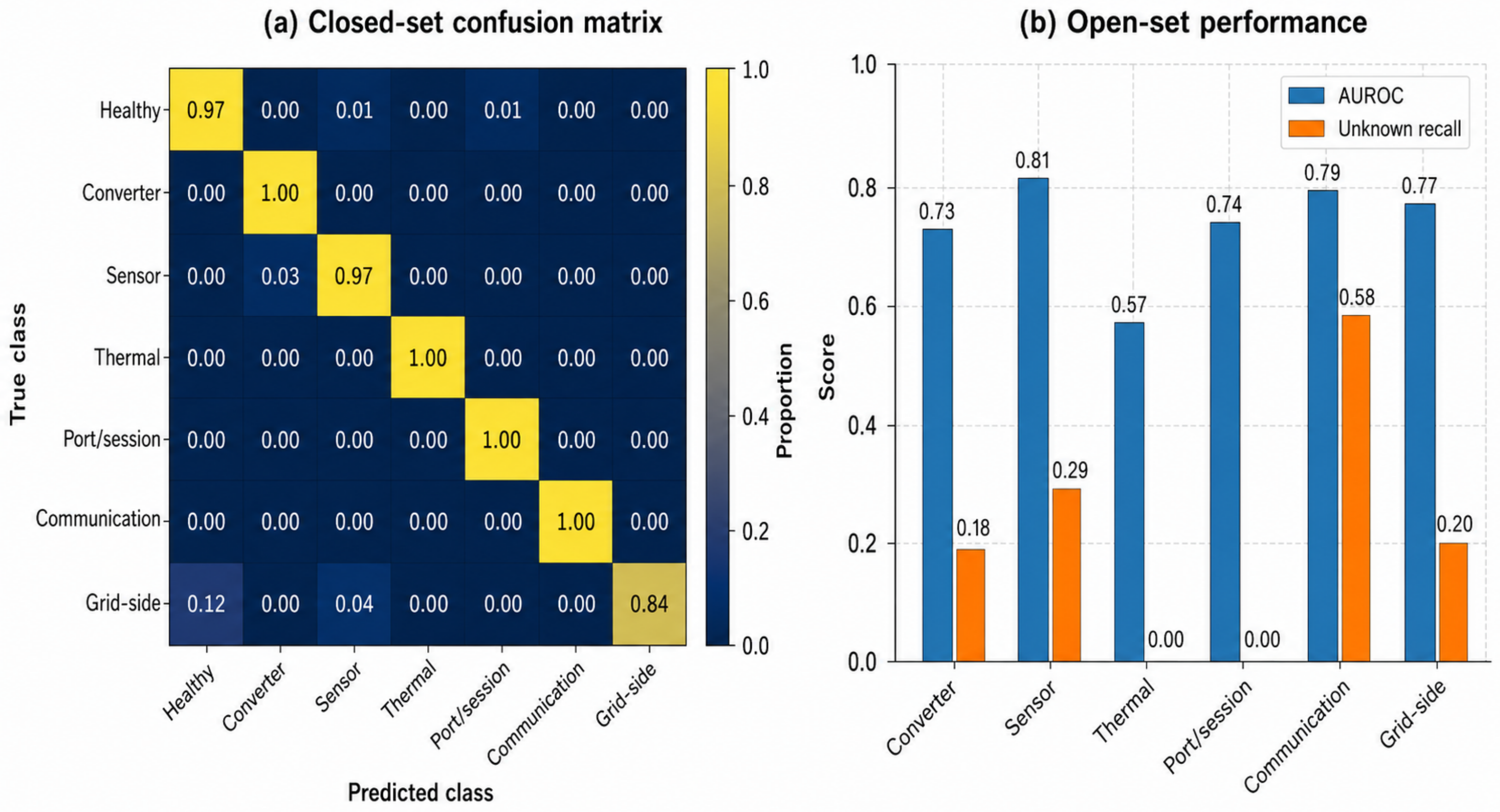
Figure 4 complements the aggregate and per-class metrics by showing the pattern of closed-set classification errors and the variation in open-set detectability across held-out fault families. The closed-set confusion matrix confirms that the principal residual ambiguity involves grid-side disturbances, while the open-set panel shows that unknown-fault recognition is strongly source dependent.

Although the closed-set results are high, they should be interpreted within the controlled benchmark assumptions rather than as direct evidence of universal field performance. To reduce the risk of overinterpreting the 98.45% accuracy and 0.9792 macro-F1 values, several credibility controls were included in the evaluation design. These controls are summarized in

Table 13. Credibility controls used to contextualize the high closed-set classification performance.

Credibility Concern	Control Included in the Study	Interpretation
Possible overoptimistic closed-set accuracy	Per-class precision, recall, F1-score, support, and confusion-matrix analysis are reported.	Checks whether the result is balanced across classes rather than dominated by a majority class.
Possible dependence on one random realization	Repeated-seed evaluation is used across multiple valid benchmark realizations.	Reduces dependence on a single synthetic run.
Possible easy separation of severe injected faults	Additional hardness experiments include mild, overlapping, incipient, and mixed-fault cases.	Shows that performance decreases under more ambiguous conditions.
Possible mismatch with unseen faults	Open-set/leave-one-class-out evaluation is included.	Tests whether unseen abnormal classes can be rejected rather than forced into known labels.
Possible operational overclaim	Results are framed as controlled-benchmark evidence for decision support.	Avoids claiming field-validated predictive-maintenance performance.
Risk of event-level temporal leakage	Chronological event-level partitioning and boundary-buffer exclusion were used. Windows close to split transitions were excluded, and dominant event identifiers were not shared across partitions.	Reduces the risk that performance is inflated by adjacent overlapping windows or repeated signatures from the same injected event appearing across partitions.

. As shown in Table 13, the reported closed-set score is supported by complementary checks rather than by a single aggregate accuracy value. In particular, the per-class results verify that the model is not only exploiting the dominant normal class, while the repeated-seed, hardness, and open-set experiments define the conditions under which the diagnosis task becomes more difficult. Therefore, the high closed-set performance is best interpreted as evidence of strong separability under the defined benchmark assumptions, not as a claim of universal field accuracy across all EVCS designs and operating environments.

Table 14. Per-class performance of the Random Forest classifier used for explainability and decision-layer analysis.

Class	Precision	Recall	F1-Score	Support
Healthy operation	0.9887	0.9704	0.9794	263
Converter/open-circuit fault	0.9500	1.0000	0.9744	38
Sensor/measurement fault	0.9189	0.9714	0.9444	35
Thermal/cooling anomaly	0.9767	1.0000	0.9882	42
Port/session failure	0.9130	1.0000	0.9545	21
Communication/data anomaly	0.9667	1.0000	0.9831	29
Grid-side disturbance	1.0000	0.8400	0.9130	25

reports the per-class performance of the Random Forest model used for detailed analysis. The classifier identified most converter, thermal, port/session, communication/data, and sensor-related faults with high recall. Communication/data anomalies achieved the highest F1-score of 0.9831, followed by healthy operation, thermal/cooling anomalies, converter/open-circuit faults, and port/session failures. The lowest class-level F1-score was obtained for grid-side disturbances. This class achieved perfect precision but lower recall, indicating that when the model predicted a grid-side disturbance it was reliable, but some true grid-side events were assigned to neighboring classes. This is technically plausible because mild grid-side disturbances can partially overlap with normal voltage variability and measurement-residual behavior.

Raw time-series baselines were also evaluated to determine whether direct temporal models could replace the engineered window features. The best raw-sequence model was a 1D-CNN, which achieved 95.43% accuracy and 0.9310 macro-F1. This confirms that raw temporal models can learn useful diagnostic patterns. However, under the available labeled event data, engineered multi-source window features combined with tree or boosting models remained more effective.

Boundary-Buffer Sensitivity

To assess whether the reported LightGBM performance depends on the exact temporal exclusion margin, the chronological split was repeated using boundary buffers of 0, 30, 60, 90, and 120 min. The benchmark realization, extracted features, chronological transition locations, LightGBM configuration, and random seed were held fixed. As summarized in

Table 15. Sensitivity of LightGBM performance to the chronological boundary-buffer width.

Buffer	Excluded	Train	Val.	Test	Accuracy	Macro-F1	Common acc.	Common F1
0 min	7	1379	457	457	0.9825	0.9768	0.9822	0.9767
30 min	15	1377	453	455	0.9802	0.9749	0.9800	0.9748
60 min	23	1375	449	453	0.9845	0.9792	0.9844	0.9792
90 min	31	1373	445	451	0.9845	0.9806	0.9844	0.9806
120 min	39	1371	441	449	0.9822	0.9770	0.9822	0.9770

, the number of excluded windows increased from 7 under the zero-margin condition to 39 under the 120-min condition, corresponding to only 0.30–1.70% of the 2300 generated windows.

Across the five settings, LightGBM accuracy ranged from 0.9802 to 0.9845, while macro-F1 ranged from 0.9749 to 0.9806. The nominal 60-min buffer retained 453 test windows and reproduced the reported accuracy of 0.9845 and macro-F1 of 0.9792. Because increasing the buffer slightly changes the composition of the held-out test set, all five trained models were also evaluated on a common conservative subset of 449 test windows retained under every buffer configuration. On this fixed subset, accuracy ranged from 0.9800 to 0.9844 and macro-F1 ranged from 0.9748 to 0.9806. The maximum variation in accuracy was therefore below 0.45 percentage points, indicating that the headline closed-set result is stable and is not attributable to one specific boundary-buffer width.

4.2. Value of Multi-Source Monitoring

The second experiment evaluates whether multi-source monitoring provides measurable value over conventional electrical-only fault diagnosis.

Table 16. Feature-source ablation results using the Random Forest classifier.

Feature Set	Number of Features	Accuracy	Macro-F1
Electrical only	37	0.8433	0.6922
Electrical + thermal	57	0.9183	0.8043
Electrical + thermal + session/port	100	0.9470	0.9251
Electrical + thermal + session/port + grid/PV/BESS	151	0.9470	0.9296
Full multi-source	176	0.9735	0.9626

reports the feature-source ablation results using the Random Forest classifier. Electrical-only features achieved 84.33% accuracy but only 0.6922 macro-F1, showing that electrical measurements alone were insufficient for balanced classification across the heterogeneous fault classes. Adding thermal features improved macro-F1 to 0.8043, confirming the value of temperature and thermal-residual information. Adding session and port features produced a larger improvement, increasing macro-F1 to 0.9251. Including grid/PV/BESS features increased macro-F1 slightly to 0.9296, while the full multi-source configuration achieved the best overall result, with 97.35% accuracy and 0.9626 macro-F1.

The temporary decrease after adding grid/PV/BESS features without communication/data features is also informative. Grid/PV/BESS variables introduce additional operating variability related to PV availability, BESS dispatch, and grid import. When communication/data features are absent, this variability can overlap with healthy and communication-related behavior, reducing communication/data anomaly recall. Once communication/data features are added, this ambiguity is reduced and the full multi-source model achieves the highest macro-F1. This result supports the central premise of the paper: EVCS decision support should not be treated as a purely electrical fault-diagnosis problem. Different fault sources leave signatures in different monitoring channels, and balanced diagnosis requires heterogeneous evidence.

4.3. Unknown-Fault and Anomaly Detection

Closed-set classification and feature-source ablation provide the main evidence for the value of multi-source EVCS monitoring. In particular, the Random Forest model used for explainability and decision-layer analysis improved from 0.6922 macro-F1 under electrical-only monitoring to 0.9626 macro-F1 using the full multi-source feature set, showing that balanced diagnosis depends strongly on heterogeneous EVCS observability. However, practical EVCS deployments may also experience rare or previously unseen abnormal conditions. Therefore, anomaly-detection and open-set experiments were performed as a complementary evaluation of suspicious-event flagging.

Table 17. Comparison of anomaly-detection baselines.

Model	ROC-AUC	PR-AUC	F1	Precision	Recall
PCA reconstruction error	0.9914	0.9876	0.9490	0.9208	0.9789
Conformal PCA anomaly score	0.9905	0.9833	0.9466	0.9163	0.9789
One-Class SVM	0.9873	0.9801	0.9393	0.9418	0.9368
MLP autoencoder reconstruction	0.9769	0.9637	0.9096	0.9194	0.9000
Isolation Forest	0.8980	0.8438	0.6445	0.8739	0.5105

compares the main anomaly-detection baselines. PCA reconstruction error achieved the strongest aggregate binary anomaly-detection performance, with ROC-AUC of 0.9914, PR-AUC of 0.9876, and F1-score of 0.9490. Conformal PCA anomaly scoring achieved nearly identical performance, while One-Class SVM also performed strongly, with ROC-AUC of 0.9873 and PR-AUC of 0.9801. These aggregate anomaly-detection results should be interpreted as supporting evidence for the monitoring layer, whereas the central diagnostic claim of the paper remains the improvement in balanced multi-class fault diagnosis obtained when moving from electrical-only monitoring to full multi-source monitoring.

A stricter leave-one-class-out protocol was then used to evaluate unknown-fault detection. In each fold, one fault/anomaly class was excluded from model fitting and treated as unknown during testing. The results in

Table 18. Leave-one-class-out open-set fault/anomaly detection performance across held-out unknown classes.

Held-Out Unknown Class	ROC -AUC	PR -AUC	Unknown Recall	Known FPR	FPR@ 95TPR	Open-Set Macro-F1
Converter/open-circuit fault	0.7269	0.1347	0.1842	0.2265	0.4241	0.4689
Sensor/measurement fault	0.8127	0.1737	0.2857	0.1866	0.2368	0.5155
Thermal/cooling anomaly	0.5684	0.0997	0.0000	0.1995	0.7494	0.4207
Port/session failure	0.7392	0.0838	0.0000	0.2130	0.2986	0.4288
Communication/data anomaly	0.7957	0.1360	0.5862	0.2123	0.2476	0.5588
Grid-side disturbance	0.7679	0.1107	0.2000	0.1682	0.5654	0.4918

Note: Thermal/cooling and port/session held-out cases show zero unknown recall at the selected threshold. These cases are retained to transparently report the limitations of the open-set detector.

show that open-set performance depends strongly on the held-out fault source. Sensor/measurement faults achieved the highest AUROC among the held-out classes (0.8127), while communication/data anomalies achieved the highest unknown recall at the selected threshold (0.5862). In contrast, thermal/cooling anomalies remained difficult to identify as unknown, with AUROC of 0.5684 and zero unknown recall. Port/session failures also had zero unknown recall at the selected threshold despite a higher AUROC of 0.7392, indicating a threshold-calibration limitation. These results show that the open-set layer is useful for suspicious-event flagging, but unknown-fault rejection remains uneven across fault sources. In particular, unknown faults that overlap with known operating states or normal high-load behavior may require additional sensing, class-specific calibration, adaptive thresholding, or stronger thermal/session modeling before they can be reliably rejected as unseen events.

These results are important for interpreting the scope of the framework. The anomaly layer should be viewed as decision support for suspicious-event flagging, not as a guarantee of complete unknown-fault coverage. It is most useful when the unknown event produces a distinctive feature pattern, while fixed validation-selected thresholds remain less reliable for fault sources that overlap with known classes or normal operating variability.

Unknown mixed-fault cases were also evaluated. Thermal–sensor, communication–port, and grid–converter compound faults were detected at high rates by the anomaly layer, indicating that compound abnormal conditions tend to produce stronger deviations than some single held-out classes. Distribution-shifted but non-fault normal scenarios produced substantially lower false unknown rates, suggesting that the open-set layer is not merely reacting to any operating variation. Nevertheless, additional field validation is required before deploying such thresholds in operational EVCS networks.

4.4. Explainability and Source-Evidence Consistency

The explainability analysis evaluates whether the diagnostic evidence used by the model is consistent with the expected physical or operational origin of each fault class. Grouped feature-source importance showed that the Random Forest model did not rely on a single signal family. The source ranking was communication/data, session/port, electrical, thermal, and grid/PV/BESS, with mean grouped importances of 0.2683, 0.2464, 0.2077, 0.1757, and 0.1020, respectively, across repeated model seeds. The ranking was stable across seeds, supporting the robustness of the source-level explanation.

Different explanation methods produced different global source rankings. Native tree-impurity importance ranked communication/data first, permutation importance ranked grid/PV/BESS first, and TreeSHAP aggregation ranked session/port first. This variation is expected because impurity reduction measures model split usage, permutation importance measures predictive-performance degradation, and TreeSHAP distributes prediction attribution across correlated features.

To quantify their common evidence, the three rankings were aggregated using the Borda procedure defined in Section 3.9. As shown in

Table 19. Borda consensus of the global monitoring-source rankings produced by the three explanation methods.

Source Group	Native	Permutation	TreeSHAP	Borda Score	Consensus Rank
Communication/data	1	3	2	9	1
Session/port	2	5	1	7	2 (tie)
Electrical	3	2	3	7	2 (tie)
Grid/PV/BESS	5	1	5	4	4
Thermal	4	4	4	3	5

, communication/data obtained the highest consensus score of 9, corresponding to a normalized score of 0.750. Session/port and electrical evidence were tied in the second consensus tier, each with a score of 7. Grid/PV/BESS and thermal evidence ranked fourth and fifth, respectively. The consensus therefore identifies communication/data as the strongest station-wide source group but does not support a unique second-ranked source.

The global consensus ranking should not be interpreted as a fault-specific causal diagnosis. Instead, it indicates which monitoring sources are influential across the complete test set and is useful for model auditing and monitoring-system prioritization. Operational candidate-source interpretation remains class conditioned: the dominant and secondary sources in

Table 20. Dominant and secondary diagnostic-evidence source groups obtained from the class-wise source-shift map.

Fault Class	Dominant Source	Secondary Source
Converter/open-circuit fault	Electrical	Session/port
Sensor/measurement fault	Electrical	Communication/data
Thermal/cooling anomaly	Thermal	Grid/PV/BESS
Port/session failure	Session/port	Grid/PV/BESS
Communication/data anomaly	Communication/data	Electrical
Grid-side disturbance	Grid/PV/BESS	Electrical

are used to guide inspection for the predicted fault class. When no clear source is supported, the framework should retain multiple candidate sources and require operator review rather than collapse the evidence into a potentially misleading single-source explanation.

Table 20 summarizes the dominant and secondary source groups in the class-wise source-shift map. Converter/open-circuit faults and sensor/measurement faults were dominated by electrical features. Thermal/cooling anomalies were dominated by thermal features. Port/session failures were dominated by session/port features. Communication/data anomalies were dominated by communication/data features. Grid-side disturbances were dominated by grid/PV/BESS features, with a secondary electrical contribution. This behavior is important because a high-accuracy black-box classifier alone is insufficient for maintenance decision support. Operators need to know whether an alarm is mainly electrical, thermal, port-related, communication-related, or grid-related.

Figure 5 visualizes the distinction between global model-level explanation and class-conditioned inspection guidance. Panel (a) compares the source rankings produced by native impurity importance, permutation importance, TreeSHAP, and their Borda consensus. Panel (b) shows the normalized class-wise source-shift map used to identify the dominant and secondary inspection sources for each fault class.

4.5. Maintenance Decision Support and Operational Impact

The diagnostic outputs were converted into maintenance-oriented health states using the heuristic risk-score layer described in Section 3. The purpose of this layer is not to claim a deployable or operator-calibrated maintenance policy, but to evaluate how diagnostic outputs can be translated into interpretable decision-support states.

Table 21. Comparison of representative maintenance decision policies.

Policy	Availability Gain (pp)	Unavailable-Hour Reduction (%)	Unmet-Energy Reduction (%)	Action Precision	Action Recall
Anomaly-threshold-only rule	1.216	49.01	37.86	0.9418	0.9368
Nominal risk-score decision layer	1.216	49.01	38.33	0.9307	0.9895
Confidence-only non-healthy rule	1.067	42.98	33.12	1.0000	0.6421
Severity-only rule	1.067	42.98	34.59	0.9623	0.5368
Threshold-only operational-impact rule	0.691	27.84	20.69	1.0000	0.1158
Reactive-only policy	0.000	0.00	0.00	0.0000	0.0000

compares the nominal risk-score layer with alternative decision policies. The reactive-only policy produced no avoided service degradation. The nominal risk-score layer improved port availability by 1.216 percentage points, reduced unavailable port hours by 49.01%, and reduced unmet charging energy by 38.33%. The anomaly-threshold-only rule produced a similar unavailable-hour reduction and slightly lower unmet-energy reduction. Confidence-only, severity-only, and threshold-only operational-impact rules also reduced service loss, but with different trade-offs between action precision and action recall. These results should be interpreted as a policy-response simulation conditioned on assumed intervention effectiveness, not as an empirical estimate of scenario-based operational benefits.

To determine whether the operational conclusions depend on the specific coefficients in Equation (14), the decision layer was evaluated under alternative component-priority schemes and 100 randomly perturbed non-negative weight vectors constrained to sum to one. The random vectors were sampled from a Dirichlet distribution centred on the nominal vector, $({\mathbf{w}}^{\left(b\right)}\sim \mathrm{Dirichlet}\left(80{\mathbf{w}}_0\right))$, thereby testing moderate variations around the stated engineering priorities without using test outcomes to select the coefficients. As summarized in

Table 22. Sensitivity of operational conclusions to the risk-score weight choices.

Weight Setting	Availability Gain	Unavailable-Hour	Unmet-Energy	Action	Mean Delay
	(pp)	Reduction (%)	Reduction (%)	Precision	(min)
Nominal weights	1.216	49.01	38.33	0.9307	18.75
Equal weights	1.216	49.01	38.33	0.9307	18.75
Severity-prioritized	1.216	49.01	37.49	0.9400	20.63
Monte Carlo mean	1.212	48.83	38.13	0.9325	19.12

, the equal-weight configuration produced the same unavailable-port-hour and unmet-energy reductions as the nominal vector. A severity-prioritized configuration slightly reduced unmet-energy recovery and increased detection delay, but retained the same unavailable-port-hour reduction. Across the 100 random weight vectors, the mean unavailable-port-hour reduction was 48.83% and the mean unmet-energy reduction was 38.13%, compared with 49.01% and 38.33% under the nominal vector. These results indicate that the main operational conclusion is not sensitive to one exact set of coefficients.

The operational-response results must be interpreted carefully. The reactive case produced 2.86 unavailable port hours and 235.70 kWh of unmet charging energy over the held-out evaluation period. The nominal 49.01% unavailable-hour reduction and 38.33% unmet-energy reduction correspond to one generic response assumption in which the remaining unavailable-port duration is reduced by 50% and the remaining unmet charging energy is reduced by 40% after early detection. These values are not field-measured scenario-based operational benefits. They represent one operating point in a scenario-based response-sensitivity analysis.

To make the fault-type-specific response model explicit,

Table 23. Fault-type-specific operational-response assumptions used in the scenario-based response analysis.

Fault Class	Expected Response/Intervention Type	Delay (min)	Remote Success	Downtime Reduction	Unmet-Energy Reduction
Converter/ open-circuit fault	Derate charger, isolate affected converter, inspect power module	90	0.35	0.25	0.20
Sensor/ measurement fault	Fallback sensing, recalibration check, acquisition-chain inspection	20	0.60	0.35	0.20
Thermal/ cooling anomaly	Thermal derating, cooling-path inspection, fan/filter cleaning	45	0.50	0.45	0.30
Port/session failure	Port reset, port isolation, user rerouting, connector inspection	30	0.65	0.55	0.45
Communication/ data anomaly	Remote communication reset, backend validation, data-quality recovery	10	0.80	0.70	0.35
Grid-side disturbance	BESS support, grid-aware charging reduction, operator/grid notification	15	0.55	0.30	0.25

summarizes the assumed intervention type, response delay, remote-success probability, and effectiveness parameters used for each fault class. These values are not field-calibrated maintenance parameters. They are scenario assumptions used to test how the same diagnostic outputs would translate into different operational outcomes when the remediation dynamics differ by fault source.

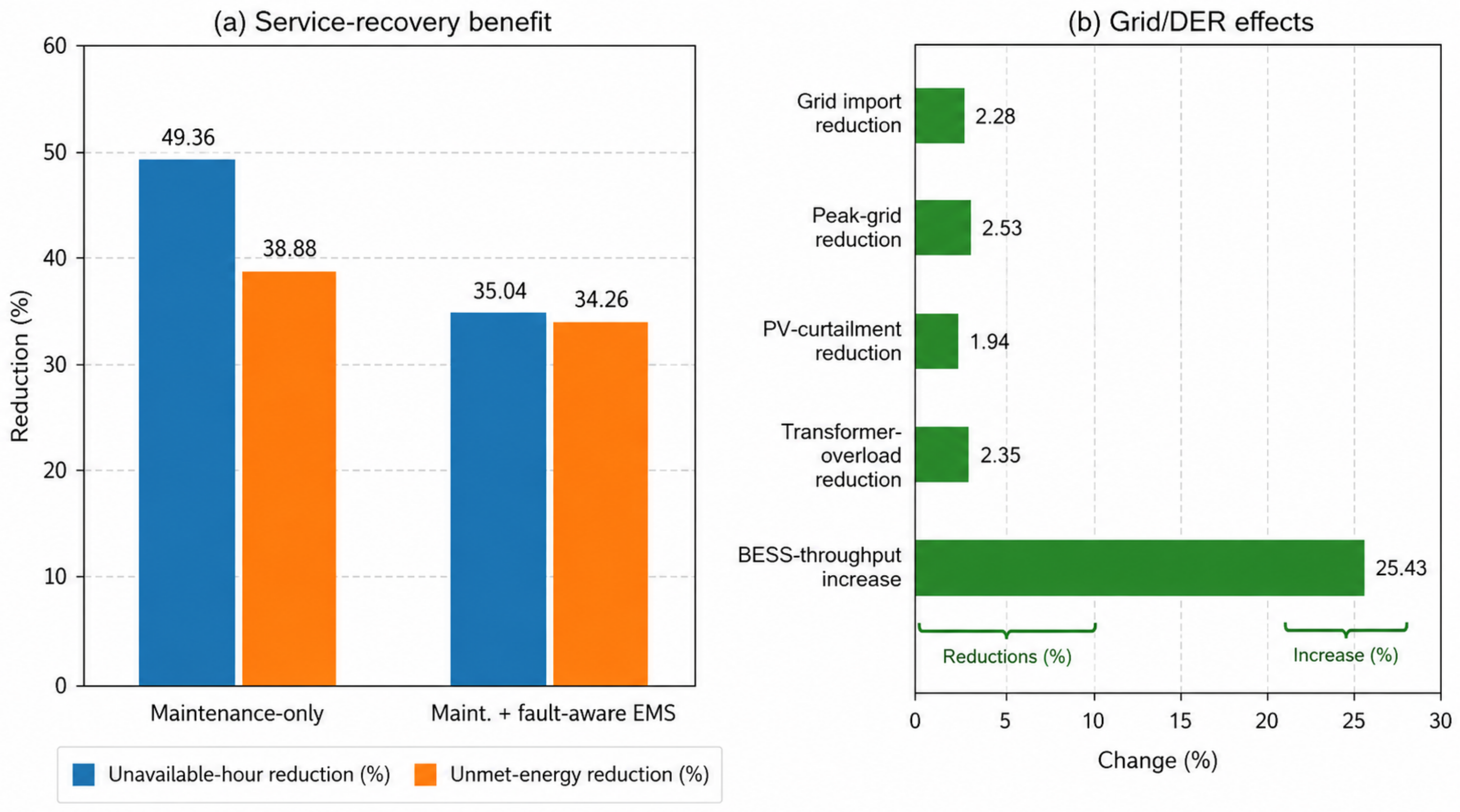
Figure 6 visualizes the different objectives of the maintenance-only and DER-aware policies. The maintenance-only policy provides the largest immediate service-recovery benefit, whereas the DER-aware policy sacrifices part of that benefit to reduce grid and transformer stress and increase BESS support.

Using these assumptions, the fault-type-specific action model produced more conservative reductions than the nominal generic response because some faults require longer response delays, lower remote-success probability, or partial remediation only.

Table 24. Sensitivity of operational-response outcomes to intervention effectiveness and response delay.

Policy/Scenario	Delay (min)	Avail. Gain (pp)	Unavail.-Hour Reduction (%)	Unmet-Energy Reduction (%)	Intervention Rate
Low-effectiveness generic response (20/20)	0	0.49	19.60	19.17	1.0000
Nominal generic response (50/40)	0	1.22	49.01	38.33	1.0000
Optimistic generic response (60/60)	0	1.46	58.81	57.50	1.0000
Maintenance crew delay (50/40 + 60 min)	60	0.62	24.88	21.54	0.9375
Spare-part delay (50/40 + 120 min)	120	0.20	7.90	8.53	0.5625
Fault-type-specific action model	Type-specific	0.66	26.42	15.78	0.8125

then summarizes the sensitivity of the operational benefit to intervention effectiveness and response delay. Under a low-effectiveness generic response, unavailable-port reduction decreased to 19.60% and unmet-energy reduction to 19.17%. Under an optimistic response, the corresponding reductions increased to 58.81% and 57.50%. Introducing a 60-min maintenance-crew delay reduced the benefit to 24.88% unavailable-hour reduction and 21.54% unmet-energy reduction, while a 120-min spare-part delay reduced the benefit further. The fault-type-specific action model produced more conservative reductions because different fault classes were assigned different delays, success probabilities, and remediation effects.

Because the EVCS is renewable-powered and grid-interactive, an additional DER-aware response scenario was evaluated.

Table 25. Comparison of reactive operation, maintenance-only response, and DER-aware response.

Scenario	UHR	UER	GIR	PGR	PCR	TOR	BTI
Reactive operation	0.00	0.00	0.00	0.00	0.00	0.00	0.00
Maintenance-only	49.36	38.88	0.00	0.00	0.00	0.00	0.00
Maint. + fault-aware EMS	35.04	34.26	2.28	2.53	1.94	2.35	25.43

UHR: Unavailable-hour reduction (%); UER: Unmet-energy reduction (%); GIR: Grid-import reduction (%); PGR: Peak-grid reduction (%); PCR: PV-curtailment reduction (%); TOR: Transformer-overload reduction (%); BTI: BESS-throughput increase (%).

compares reactive operation, maintenance-only response, and maintenance response coupled with fault-aware energy management. The maintenance-only response reduced unavailable port hours and unmet energy but left grid import, peak grid import, PV curtailment, and BESS throughput unchanged because no DER redispatch was modeled. The DER-aware scenario reduced grid import by 2.28%, peak grid import by 2.53%, and PV curtailment by 1.94%, while increasing BESS throughput by 25.43%.

The DER-aware scenario should not be interpreted as uniformly superior to maintenance-only operation. Relative to the maintenance-only policy, unavailable-hour recovery decreased from 49.36% to 35.04%, corresponding to a 14.32-percentage-point reduction in service-recovery benefit. Unmet-energy recovery also decreased by 4.62 percentage points, from 38.88% to 34.26%. This service penalty resulted from protective charging derating and delayed restoration during converter, thermal, and grid-side events.

In exchange, the DER-aware scenario reduced total grid import by 2.28%, peak grid import by 2.53%, PV curtailment by 1.94%, and transformer-overload exposure by 2.35%, while increasing BESS throughput by 25.43%. These values describe an operational trade-off rather than a net economic benefit. In particular, the increase in BESS throughput may introduce additional cycling and degradation costs that must be included in a site-specific economic assessment.

Accordingly, the maintenance-only policy is the appropriate default when grid and thermal constraints are inactive and rapid service restoration is the dominant objective. The DER-aware policy becomes justified when continued full-power recovery would violate equipment-temperature limits, increase transformer-overload exposure, exceed a contracted demand limit, incur a sufficiently high peak-demand charge, or cause material renewable-energy curtailment. Under such conditions, temporary loss of charging availability may be accepted to avoid a larger asset, safety, or grid-service cost. The break-even condition is that the monetary value of avoided grid-energy, peak-demand, curtailment, and transformer-risk costs exceeds the added cost of unavailable-port time, unmet charging demand, and BESS cycling.

Because the present benchmark does not include site-specific tariffs, customer-compensation costs, battery-degradation prices, or transformer-failure costs, it cannot determine a universally optimal policy. Table 25 therefore illustrates the Pareto trade-off between service recovery and grid/asset protection rather than demonstrating economic superiority of the DER-aware policy. In deployment, the coefficients of the cost function introduced in Section 3.10 should be calibrated using local tariffs, service-level agreements, BESS degradation models, transformer limits, and operator risk preferences.

4.6. Robustness, Extended-Horizon Evaluation, and Computational Feasibility

Robustness was evaluated by perturbing the held-out test features with increasing fractions of the training-set standard deviation. The Random Forest classifier maintained strong performance under all tested noise levels. At the highest noise fraction of 0.15, it still achieved 94.04% accuracy and 0.9155 macro-F1. This result indicates that the classifier retains substantial diagnostic performance under feature perturbations within the tested range.

The full Random Forest-based explainability and decision-support pipeline was also repeated over five valid stochastic benchmark realizations. A valid realization was defined as a generated benchmark in which all operating and fault classes were represented in the held-out test windows. Across these runs, the mean Random Forest macro-F1 was 0.9461 with a standard deviation of 0.0202. The One-Class SVM achieved mean ROC-AUC of 0.9854 and mean PR-AUC of 0.9739. The event detection rate remained 1.0000 across valid realizations, with a mean detection delay of 17.66 min. The mean unavailable-port-hour reduction was 46.71%, and the mean unmet-energy reduction was 37.16%. These repeated-seed results assess the stability of the Random Forest-based explanation and decision-support pipeline, together with the anomaly-detection and operational-response layers. They should not be interpreted as a repeated-seed estimate of the headline LightGBM result, which was evaluated in the main single-seed held-out comparison.

The extended-horizon benchmark further evaluated event-level behavior over 180 days. The held-out extended-horizon test set contained 81 events, all 81 injected test events satisfied the specified event-level detection criterion. The mean detection delay was 10.80 min, and the mean detection lead time was 130.68 min. This event-level detection rate should be interpreted differently from window-level classification or open-set recognition, because each injected event spans multiple consecutive windows and is counted as detected if at least one window within the event is flagged before or during the event interval. Detection delays varied by fault class: sensor/measurement faults and port/session failures were detected more rapidly, while grid-side disturbances had the longest mean delay. This is consistent with the nominal benchmark, where grid-side disturbances were more difficult because their signatures partially overlapped with normal operating variability.

The hardness, repeated-seed, noise-perturbation, and extended-horizon experiments evaluate different aspects of synthetic-data representativeness. The hardness experiments test whether performance persists when fault signatures become weaker or overlap; repeated seeds test dependence on one stochastic realization; feature perturbation tests sensitivity to measurement uncertainty; and the 180-day benchmark tests longer-term operational variation. These experiments strengthen internal validity, but they do not establish external validity because all observations remain generated by the same modeling assumptions. Field validation is therefore still required to assess distribution shift, vendor-specific behavior, real fault prevalence, and maintenance-confirmed diagnostic performance.

Computational feasibility was also assessed. The full simulation, feature extraction, model training, anomaly detection, explainability, maintenance-decision generation, robustness evaluation, operational-impact assessment, and figure generation pipeline required 9.48 s on the test machine. The Random Forest model required approximately 0.107 ms per window for inference. This inference time is negligible relative to the 5-min sampling interval and 1-h analysis window used in the benchmark, indicating that the proposed diagnostic layer is computationally feasible for near-real-time window-based EVCS monitoring. Field deployment would still require integration with charger telemetry, station-management systems, cybersecurity controls, and operator workflows.

4.7. Discussion of Main Findings and Limitations

The results support four main findings. First, multi-source monitoring substantially improves EVCS fault diagnosis compared with electrical-only monitoring. The improvement from 0.6922 macro-F1 using electrical-only features to 0.9626 macro-F1 using the full multi-source feature set shows that heterogeneous EVCS faults cannot be captured reliably by one signal family. Second, imbalance-aware gradient-boosting models provide the strongest closed-set performance, but Random Forest remains suitable for explanation and decision-layer analysis because it combines high macro-F1 with interpretable feature-source importance. Third, open-set detection is useful but uneven. Communication/data and sensor/measurement faults are more separable as unknown classes, whereas thermal, converter, port/session, and grid-side unknowns are more difficult at the selected threshold. Fourth, diagnostic outputs can support operational decision-making, but the magnitude of the service benefit depends strongly on intervention effectiveness, response delay, and fault-type-specific remediation assumptions.

4.7.1. Comparison with Existing Literature and Demonstrated Advances

Table 26. Task-level comparison with representative EVCS fault-diagnosis, anomaly-detection, explainability, and maintenance-decision studies. Reported results are contextual rather than directly rankable because the datasets, fault definitions, and evaluation protocols differ.

Study/Task	Evidence and Reported Result	Main Scope Limitation	Advance in the Present Study
Chen et al. [6]	DC charging-station open-circuit diagnosis using S-transform features and LightGBM with simulated and experimental fault data; 97.04% average diagnostic accuracy.	Component-specific electrical-fault diagnosis without station-wide multi-source monitoring, open-set evaluation, risk mapping, or operational-response analysis.	Extends the evaluation to healthy operation and six heterogeneous EVCS fault families, together with source ablation, unknown-event detection, risk-state mapping, and operational assessment.
Xu et al. [9]	Deep multifeature fusion for charging-pile open-circuit diagnosis; 96.36% diagnostic accuracy.	Focuses on converter open-circuit fault categories and detailed electrical signal fusion.	Broadens the evidence space to electrical, thermal, session/port, grid/PV/BESS, and communication/data sources.
Duan et al. [8]	Spatiotemporal feature fusion for non-intrusive charging-pile fault identification using simulated multi-capacity data; macro-average improvements of 2.99% over Random Forest and 7.28% over GBDT.	Does not connect fault identification to open-set evaluation, explanation consensus, maintenance-oriented risk states, or operational-response analysis.	Adds chronological evaluation, source ablation, leave-one-class-out testing, mixed-fault analysis, explanation consensus, and operational mapping.
Sakwa et al. [11]	Autoencoder- and LSTM-based analysis of EVSE charging-power profiles in a real-world case study; early anomaly-detection capability was demonstrated.	Provides profile-level anomaly evidence without labeled multiclass station diagnosis, source-level interpretation, or maintenance-state mapping.	Combines anomaly detection with known-fault classification, source-oriented interpretation, risk states, and scenario-based operational consequences.
Cederle et al. [24]	Isolation Forest with DIFFI explanation using real-world sensor and charging-session data; anomalous sessions and influential features were identified.	Explainable unsupervised analysis without integrated closed-set diagnosis, maintenance-risk scoring, or grid/DER-response assessment.	Combines impurity importance, permutation importance, and TreeSHAP with Borda consensus, class-conditioned source evidence, and human-review logic.
Cai et al. [26]	Lifecycle- and safety-based preventive-maintenance decision optimization; up to 98% decision accuracy and an average decision time of 1.6 s.	Uses lifecycle, failure-probability, outage, and maintenance-timing factors rather than window-level multi-source diagnostic evidence.	Links multi-source fault diagnosis to source-aware health states and service/DER-response scenarios.
Present study	Seven-class multi-source EVCS diagnosis, open-set detection, explainability, risk mapping, and operational-response assessment; 98.45% accuracy and 0.9792 macro-F1. Random Forest macro-F1 increased from 0.6922 with electrical-only monitoring to 0.9626 with full multi-source monitoring.	Controlled synthetic benchmark; field generalization, economic benefit, causal fault-source identification, and autonomous operational applicability remain unvalidated.	Provides an integrated and reproducible assessment of heterogeneous fault diagnosis, unknown-event behavior, explanation consistency, maintenance-oriented states, and service/grid consequences.

compares the present results with representative EVCS fault-diagnosis, anomaly-detection, explainability, and maintenance-decision studies. The numerical values should not be interpreted as a common leaderboard because the studies use different datasets, fault families, signal resolutions, train–test protocols, and prediction targets. The comparison is therefore used to identify task-level differences and demonstrated advances rather than to claim direct numerical superiority.

Component-specific diagnostic studies have reported high classification performance. Chen et al. [6] obtained an average diagnostic accuracy of 97.04% for open-circuit faults in a DC charging station using improved S-transform features and LightGBM, including experimental fault data. Xu et al. [9] reported 96.36% accuracy using a deep multifeature-fusion model for charging-pile open-circuit diagnosis. Duan et al. [8] reported that their spatiotemporal fusion approach improved the macro-average score by 2.99% and 7.28% over Random Forest and gradient-boosted decision-tree baselines, respectively. These studies provide strong evidence for identifying specific electrical or converter fault modes, whereas the present benchmark covers six heterogeneous infrastructure-fault families together with healthy operation.

Anomaly-oriented studies address a different but complementary objective. Sakwa et al. [11] used autoencoder and LSTM-based analysis of EVSE power profiles for early anomaly detection in a real-world case study. Cederle et al. [24] combined Isolation Forest with depth-based feature importance to detect and interpret anomalous charging behavior using real-world sensor and session data. These studies provide valuable field-oriented anomaly evidence, but they do not jointly evaluate known-fault classification, leave-one-class-out unknown-fault detection, multiple explanation methods, risk-state mapping, and service/DER consequences.

Maintenance-oriented studies also differ in their inputs and objectives. Cai et al. [26] reported preventive-maintenance decision accuracy of approximately 98% and an average decision time of 1.6 s using lifecycle, safety-failure, outage, and maintenance-timing factors. In contrast, the present decision layer begins with window-level multi-source diagnostic evidence and translates it into source-aware health states and scenario-based service and DER-response indicators. The two reported accuracy values are therefore not directly comparable: one evaluates lifecycle-based maintenance decisions, while the present 98.45% result evaluates seven-class operating and fault-state classification.

Within these limitations, five advances were demonstrated. First, the study expands the diagnostic scope from a single component or signal family to electrical, thermal, session/port, grid/PV/BESS, and communication/data-quality evidence. Full multi-source monitoring increased the Random Forest macro-F1 from 0.6922 under electrical-only monitoring to 0.9626, an absolute improvement of 0.2704. Second, the best closed-set configuration achieved 98.45% accuracy and 0.9792 macro-F1 across healthy operation and six infrastructure-fault families under chronological hold-out evaluation. Third, leave-one-class-out and mixed-fault experiments showed that unknown-fault detectability is source dependent rather than uniformly strong: sensor and communication anomalies were more detectable, whereas thermal/cooling and port/session unknowns remained difficult. Fourth, the study combines native importance, permutation importance, TreeSHAP, and Borda rank consensus with class-conditioned source shifts, thereby distinguishing global model auditing from event-level inspection guidance. Fifth, diagnostic outputs were propagated into maintenance-oriented risk states and explicit service/DER-response scenarios. Under the nominal maintenance-response assumptions, unavailable port hours and unmet charging energy decreased by 49.01% and 38.33%, respectively, while the DER-aware analysis exposed a measurable trade-off between service recovery and grid/asset protection.

The main advance is therefore not a claim that 98.45% is universally better than every reported EVCS diagnostic result. Rather, it is the demonstration that competitive closed-set performance can be retained while broadening the evaluation to heterogeneous fault sources, open-set behavior, explanation consistency, maintenance-oriented state mapping, and operational consequences. External validation remains necessary because the present results are obtained from a controlled synthetic benchmark, whereas several related studies use narrower but experimentally measured or field-collected datasets.

4.7.2. Conceptual, Methodological, and Practical Contributions

The principal conceptual and methodological contribution is the integration of previously separate EVCS health-management functions within a unified decision-support structure. Existing EVCS research commonly treats component-level fault diagnosis, anomaly detection, explainability, renewable-energy operation, and maintenance planning as separate problems. The proposed framework establishes an integrated representation in which these elements are connected through five stages: multi-source observability, hybrid closed- and open-set diagnosis, source-level explanation, maintenance-oriented risk mapping, and operational-response assessment. This formulation extends EVCS fault analysis beyond the prediction of a class label by defining how diagnostic evidence can be interpreted and propagated into decision-support states. The source-structured representation and class-conditioned explanation procedure further provide a systematic means of distinguishing electrical, thermal, session/port, grid/PV/BESS, and communication/data evidence. The Borda consensus analysis adds a model-auditing mechanism when alternative explanation methods produce different global rankings, while preserving class-specific evidence for individual fault interpretation.

The practical contribution is an operator-oriented workflow for renewable-powered EVCS monitoring. The framework identifies known fault classes, flags suspicious unknown events, indicates the dominant and secondary evidence sources, and maps the results into Healthy, Warning, Degraded, and Critical states. These outputs can support inspection prioritization, charger derating decisions, affected-port isolation, communication diagnostics, cooling-system inspection, and grid-aware operating responses, subject to operator review. The feature-source ablation also indicates which monitoring groups provide the greatest diagnostic value and can therefore inform sensing and data-acquisition design. In addition, the service-response and DER-aware analyses quantify the trade-off among port availability, unmet charging energy, grid import, peak demand, PV curtailment, transformer exposure, and BESS use. The released benchmark, configuration files, random seeds, and analysis scripts provide a reproducible basis for comparing future diagnostic and decision-support methods. These practical contributions remain controlled-benchmark demonstrations and require calibration using field telemetry, maintenance records, site tariffs, protection constraints, and operator-specific intervention policies before deployment.

4.7.3. Current Limitations and Future Research

The proposed framework has several limitations. First, the benchmark is based on controlled simulation and fault injection rather than field-calibrated failure distributions, maintenance-confirmed labels, or long-term charger-controller records. Although the benchmark preserves physically interpretable signal relationships and includes harder fault signatures, repeated stochastic realizations, measurement perturbations, and an extended 180-day horizon, these experiments establish internal robustness rather than statistical equivalence to deployed EVCS fleets. Vendor-specific converter behavior, protection logic, charger firmware, communication delays, correlated subsystem failures, irregular user demand, and site-specific maintenance practices may therefore introduce distribution shifts not represented in the present benchmark.

Second, the temporal resolution is intended for station-level condition monitoring rather than protection-level fault detection. The 5-min sampling interval and 1-h analysis window are suitable for persistent operational abnormalities, but they may not capture fast switching faults, short protection events, arc faults, or rapidly developing thermal incidents. Higher-frequency electrical and thermal measurements, event-triggered sampling, and multiresolution models would be required for such applications.

Third, open-set detection was not uniformly effective across fault families. Unknown sensor and communication anomalies were comparatively detectable, whereas held-out thermal/cooling and port/session faults were more difficult at the selected threshold. The anomaly layer should therefore be interpreted as a suspicious-event flag rather than a complete unknown-fault recognition mechanism. Future work should investigate class-conditional thresholds, adaptive conformal methods, deep one-class models, self-supervised representation learning, and online adaptation under seasonal and equipment-ageing drift.

Fourth, the explainability and risk-mapping layers remain decision-support mechanisms rather than causal or safety-certified decision systems. Feature importance and SHAP values identify statistical evidence used by the model but do not prove the physical cause of an event. Similarly, the risk weights, severity scores, and health-state thresholds were defined using transparent engineering assumptions and sensitivity analysis, but they have not been calibrated using operator costs, safety records, service-level agreements, or maintenance outcomes. Field deployment would require probabilistic calibration, human-in-the-loop validation, alarm aggregation, uncertainty reporting, and fail-safe rules that prevent diagnostic outputs from directly initiating safety-critical isolation, shutdown, or maintenance actions without authorized review.

Real-world deployment also requires reliable integration with charger telemetry, OCPP messages, charger-controller fault codes, station-management platforms, cybersecurity controls, and maintenance workflows. Practical challenges include heterogeneous vendor data schemas, missing or delayed measurements, timestamp synchronization, firmware changes, communication outages, privacy requirements, secure model updates, and operator acceptance. A staged deployment pathway should therefore begin with offline validation using historical telemetry and maintenance records, followed by shadow-mode operation in which predictions are compared with operator decisions without controlling the station, and finally a supervised pilot deployment with predefined safety constraints and escalation procedures.

A further research direction is integration with broader energy-management systems. The present DER-aware assessment uses scenario-based responses rather than an optimized station controller. Future work should connect the diagnostic layer to station energy management systems, microgrid controllers, building energy-management systems, or distribution-level DER management platforms. Such integration could formulate fault-aware scheduling as a constrained optimization problem that jointly considers charging-service demand, PV availability, BESS state of charge and degradation, grid import limits, demand charges, transformer loading, carbon intensity, and maintenance risk. Model-predictive control, robust optimization, or reinforcement-learning approaches could then compare alternative actions such as charger derating, port rerouting, BESS support, charging deferral, and controlled load recovery while preserving electrical and thermal safety constraints.

External validation should proceed in stages. Real charging-profile datasets can first be used to calibrate session-duration, demand, and charger-power distributions. Battery-oriented datasets can support a separate vehicle-originated battery-risk source without conflating vehicle and station faults. The complete framework should then be evaluated using synchronized station telemetry, OCPP events, PV/BESS measurements, protection records, maintenance-confirmed infrastructure faults, intervention times, and operator decisions from multiple EVCS sites and charger vendors. Such validation is necessary before claims of generalizable diagnostic performance, economic benefit, or autonomous operational control can be made.

Overall, the framework provides a reproducible basis for connecting multi-source EVCS diagnosis with explanation, risk-state mapping, and operational-response assessment. Its present contribution is a controlled decision-support methodology rather than a field-validated maintenance or energy-management system. Progress toward deployment requires multi-site external validation, operator-calibrated decision rules, secure integration with station-management infrastructure, and supervised coupling with broader energy-management systems.

5. Conclusions

This study developed a fault-aware decision-support framework for renewable-powered electric vehicle charging stations using multi-source explainable learning. The framework connects electrical, thermal, session/port, grid/PV/BESS, and communication/data-quality monitoring with closed-set diagnosis, open-set anomaly flagging, source-aware explanation, maintenance-oriented risk mapping, and scenario-based operational-response assessment.

Demonstrated findings: Within the controlled benchmark, multi-source monitoring provided a clear diagnostic advantage over electrical-only monitoring. The LightGBM classifier achieved 98.45% accuracy and 0.9792 macro-F1 under chronological hold-out evaluation. The Random Forest model used for explanation and decision-layer analysis achieved 97.35% accuracy and 0.9626 macro-F1, compared with 84.33% accuracy and 0.6922 macro-F1 using electrical-only features. These results demonstrate strong separability of the six injected EVCS fault families under the defined simulation, windowing, and fault-injection assumptions.

The experiments also demonstrated that unknown-fault detection was source dependent. Sensor/measurement and communication/data abnormalities were comparatively detectable, whereas held-out thermal/cooling and port/session faults remained difficult at the selected threshold. The anomaly layer should therefore be interpreted as a suspicious-event flag, not as a complete solution for unknown-fault recognition. Source-level explanations were generally consistent with the injected fault mechanisms, and the Borda consensus procedure provided a model-auditing mechanism when global explanation methods produced different source rankings. These explanation results identify statistical evidence used by the models; they do not establish physical causality.

The risk and operational-response analyses demonstrated how diagnostic outputs can be translated into interpretable health states and evaluated under explicit intervention assumptions. Under the nominal response scenario, unavailable port hours and unmet charging energy were reduced by 49.01% and 38.33%, respectively, relative to the reactive baseline. These values are outcomes of a policy-response simulation and are not field-measured maintenance savings. The DER-aware analysis additionally demonstrated a trade-off: protective derating reduced immediate service recovery while decreasing grid import, peak demand, PV curtailment, and transformer-overload exposure and increasing BESS throughput. It did not demonstrate that the DER-aware policy is universally or economically superior.

Current evidence boundary: The demonstrated results establish benchmark-level diagnostic performance, internal robustness, explanation consistency, and the feasibility of connecting diagnosis to decision-support indicators. They do not establish generalization across charger vendors and operating sites, field-level fault-detection accuracy, causal fault-source identification, economic benefit, safety certification, or readiness for autonomous charger isolation, maintenance dispatch, or DER redispatch. The risk weights, severity values, health-state thresholds, and intervention-effectiveness parameters remain engineering-defined and require calibration using operational data.

Expected future applicability: These findings establish controlled-benchmark feasibility rather than field-level effectiveness. Multi-site validation with synchronized charger telemetry, OCPP events, protection logs, PV/BESS measurements, and maintenance-confirmed labels is required before operational deployment. Future work should prioritize adaptive open-set detection, probabilistic calibration, online adaptation, and supervised integration with station- and distribution-level energy-management systems.