A Field-Oriented Forecasting Framework for Multi-Point Dam Displacement Prediction

Abstract

Dam displacement forecasting is important for assessing whether long-term structural responses remain consistent with established operational behavior. In multi-point monitoring systems, however, irregular survey-line layouts and unequal numbers of monitoring points make it difficult to organize long-term records while preserving their engineering meaning. This study develops a field-oriented forecasting framework by reconstructing daily observations into a structured displacement-field object defined by survey-line order, monitoring-point alignment, and three displacement components. A valid-position-aware protocol is introduced to distinguish actual monitoring locations from structural padding, ensuring that model training and evaluation remain restricted to the same physical monitoring definition. Using long-term operational records from the Tianshengqiao First Dam, four representative models, namely SimVP, SimVPv2, PatchTST, and TimesNet, are evaluated under the same chronological split, causal forward-fill-only preprocessing, input window, prediction horizon, and evaluation boundary. All four models achieve strong predictive performance, with R² values above 0.97 in the X direction and above 0.99 in the Y and Z directions. No single trained model or forecasting route exhibits a consistent advantage across all displacement components and evaluation metrics. Under the present single-dam, case-specific setting, the relative ranking varies with displacement direction and forecasting horizon and should not be interpreted as evidence of general direction-specific suitability for any particular architecture. At the route level, the field-based route retains a slight advantage in Y-direction forecasting and overall MAE, whereas the sequence-based route remains competitive for Z-direction displacement and longer-horizon X-direction prediction. The proposed framework provides a practical and physically consistent digital representation for organizing irregular monitoring records, comparing forecasting routes, and supporting deployment-oriented model selection and subsequent model adaptation.

1. Introduction

Displacement monitoring provides a direct record of how a dam responds to environmental loading and operational conditions over its service life. For a dam that has been in operation for many years, the measured displacement is rarely governed by a single factor. Reservoir-level fluctuations, seasonal temperature variations, material creep, aging effects, and local differences in structural constraints may act simultaneously. Their combined influence produces deformation records with long-term trends, periodic variations, delayed responses, and stage-dependent behavior. Reliable displacement forecasting is therefore valuable not only for estimating future monitoring values, but also for determining whether the expected structural response remains consistent with the established operational pattern [1,2].

Traditional dam-displacement analysis has largely relied on statistical and empirical models. Hydrostatic–seasonal–time models and regression-based approaches remain widely used because their variables have clear engineering meanings and their results are relatively easy to interpret [1,2,3]. However, when monitoring records extend over long service periods and cover complex operating conditions, deformation responses may become increasingly nonlinear and nonstationary. Machine-learning methods can improve nonlinear fitting to some extent, but their performance often depends on manually selected variables and carefully constructed features [3,4,5]. More recently, recurrent neural networks, convolutional architectures, attention-based models, and general time-series forecasting models have provided more flexible tools for extracting temporal patterns from monitoring records [4,6,7,8,9]. Even so, the way in which the original monitoring data are organized remains a fundamental issue. A more complex model does not necessarily produce a more reliable forecast if the engineering relationships embedded in the monitoring system are weakened during data preparation.

This issue becomes particularly important in multi-point dam monitoring. Monitoring points are not installed as an arbitrary collection of sensors. They are arranged along survey lines, elevations, and characteristic structural zones to describe the coordinated deformation response of the dam body. Points located on the same survey line or at structurally related positions may exhibit similar trends, while local deviations may reflect differences in loading response, boundary constraints, or cumulative deformation behavior [10,11,12]. Treating these observations as independent time series is convenient, but it can discard information contained in the original monitoring layout. Flattening all monitoring values into a multivariate sequence preserves temporal correspondence, yet the ordered survey-line and monitoring-point arrangement is no longer represented explicitly.

A further difficulty is that engineering monitoring layouts are usually irregular. Different survey lines may contain different numbers of valid monitoring points, and long-term records may include missing observations or inconsistent baselines. Directly converting such records into a fixed-size tensor inevitably introduces padded positions that do not correspond to actual measurements. If these positions are treated as ordinary targets during model training or performance evaluation, the numerical objective no longer matches the physical boundary of the monitoring system. A suitable digital representation should therefore retain the structured monitoring layout while distinguishing valid observations from structural placeholders.

To address these issues, this study develops a field-oriented forecasting framework built on a structured digital representation of multi-point dam displacement records. Daily displacement records are reconstructed according to the original survey-line arrangement and the aligned order of monitoring points. The X-, Y-, and Z-direction displacement components are represented as separate channels, while environmental and monitoring-status information is incorporated into the same input object. A valid-position mask is introduced to identify actual monitoring locations and exclude padded positions from the official loss and evaluation boundary. The reconstructed field should not be interpreted as a complete geometric or physical model of the dam body. Instead, it is a compact engineering representation that preserves the ordered monitoring layout and provides a consistent interface between long-term monitoring records and forecasting models.

Based on this representation, two forecasting routes are examined under a unified experimental setting. The field-based route is represented by SimVP and SimVPv2 [13,14], which directly process the reconstructed displacement-field tensor and retain the structured survey-line and monitoring-point arrangement during feature extraction and prediction. The sequence-based route is represented by PatchTST and TimesNet [15,16], which reorganize the same monitoring object into multivariate temporal sequences. In the latter route, the correspondence between each variable and its original monitoring position is maintained through a fixed ordering, but the structured layout is no longer encoded explicitly during temporal modeling. The comparison is carried out under the same monitoring object, chronological data split, input window, prediction horizon, normalization procedure, and evaluation boundary. In this way, differences in forecasting behavior can be interpreted mainly in terms of the modeling route rather than inconsistencies in data processing.

The four models were selected to represent two distinct forecasting paradigms while covering different architectural characteristics within each route. SimVP provides a compact convolutional encoder–translator–decoder reference for the field-based route, whereas SimVPv2 represents an enhanced field-based architecture with gated spatiotemporal feature modeling. PatchTST represents patch-based Transformer forecasting with an emphasis on long-range temporal dependency extraction, while TimesNet represents multi-period temporal-pattern modeling through two-dimensional temporal variation. The purpose of this selection is not to identify a universally optimal architecture, but to compare how models with different inductive biases process the same multi-point monitoring object when the ordered two-dimensional layout is either explicitly retained or reformulated as a flattened multivariate temporal sequence.

The valid-position-aware protocol is also examined as a methodological component of the framework. Its purpose is not to assume that masking will necessarily improve every model, but to ensure that optimization and evaluation remain associated with actual monitoring positions. This distinction is important when different model families are compared using a common reconstructed field. By separating valid monitoring positions from structural padding, the framework provides a consistent basis for analysis within the same physical monitoring definition. The analysis covers prediction accuracy, horizon-wise stability, directional error characteristics, spatial error distributions, and engineering applicability.

The framework is evaluated using long-term monitoring data from the Tianshengqiao First Dam, a high earth–rockfill dam with a long-term operational monitoring record. The selected monitoring data include multiple survey lines and three displacement components. Historical records are reorganized into daily field samples, and a 120-day observation window is used to forecast the following 60 days. SimVP, SimVPv2, PatchTST, and TimesNet are trained and tested under the same chronological split, preprocessing procedure, prediction horizon, and valid-position-aware evaluation protocol. The purpose is not to introduce another isolated forecasting architecture, but to clarify how different data representations and modeling routes affect multi-point displacement prediction under a realistic engineering setting.

The evaluation is conducted from both numerical and engineering perspectives. In addition to overall forecasting accuracy, the analysis considers directional differences among the X-, Y-, and Z-displacement components, horizon-wise errors from t + 1 to t + 60, spatial distributions of prediction errors across the reconstructed monitoring field, and the methodological role of valid-position masking. Computational cost, inference efficiency, deployment characteristics, and update flexibility are also examined to support model selection in operational monitoring systems. Through this analysis, the study provides a practical basis for organizing irregular multi-point displacement records, comparing forecasting routes within a common physical boundary, and supporting fair model comparison and updating within the same physical monitoring definition.

The main contribution of this study is not a new forecasting architecture, but a field-oriented digital representation and a unified comparison-and-updating framework for long-term multi-point dam displacement monitoring. Within this framework, different model families can be trained, evaluated, compared, and updated under the same physical monitoring definition, the same chronological split, and the same valid-position boundary. This design allows the analysis to focus on how representation and modeling route affect forecasting behavior in an engineering setting, rather than on inconsistencies introduced by data preparation or evaluation scope.

The remainder of this paper is organized as follows. Section 2 introduces the engineering case and the field-oriented digital representation of the monitoring records. Section 3 presents the unified dual-route forecasting framework, model adaptation strategy, training protocol, and engineering-oriented evaluation method. Section 4 compares the forecasting results, horizon-wise behavior, valid-position-mask ablation results, spatial error distributions, and engineering applicability of the four models. Section 5 discusses the implications and limitations of the proposed framework, and Section 6 summarizes the main conclusions.

2. Engineering Case and Field-Oriented Digital Representation

2.1. Engineering Background and Monitoring Layout

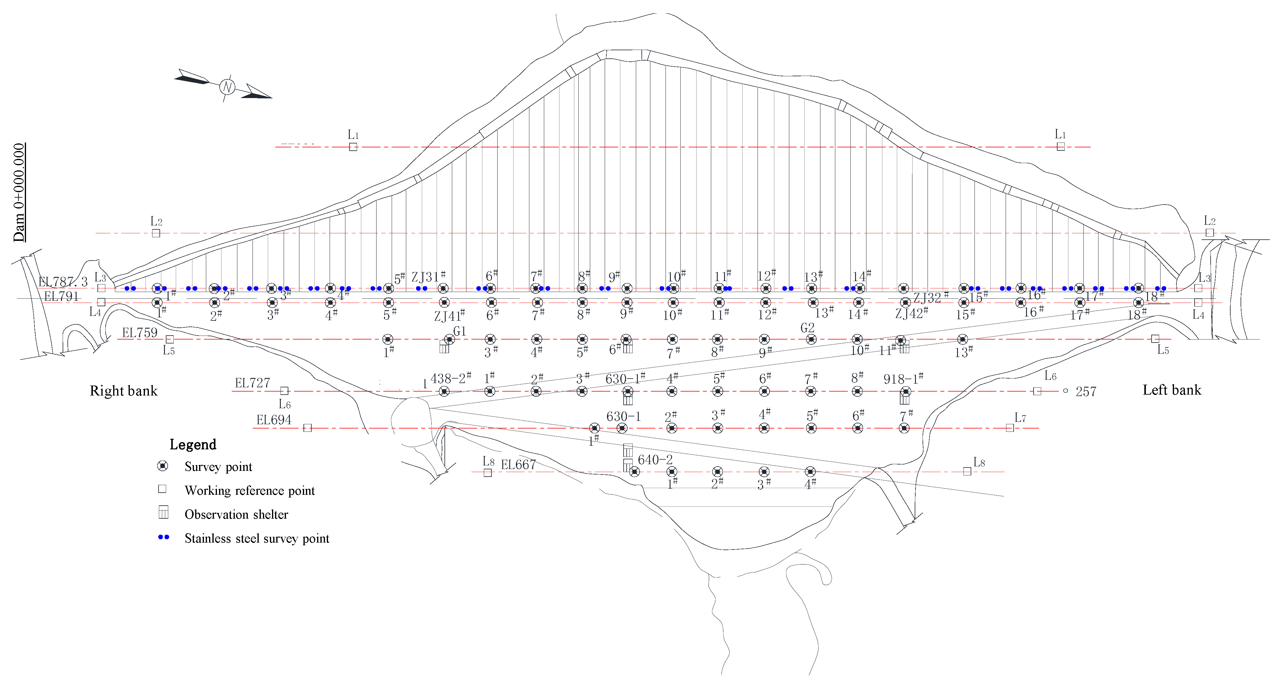
A high earth–rockfill dam was selected as the engineering case in this study. The dam has been in long-term operation for more than two decades and has experienced different operating conditions, including high reservoir water levels, flood seasons, and low-temperature periods. Its deformation monitoring records therefore provide a suitable basis for examining the performance and stability of different forecasting models in a realistic engineering setting. The spatial arrangement of the selected survey lines and displacement monitoring points is illustrated in Figure 1.

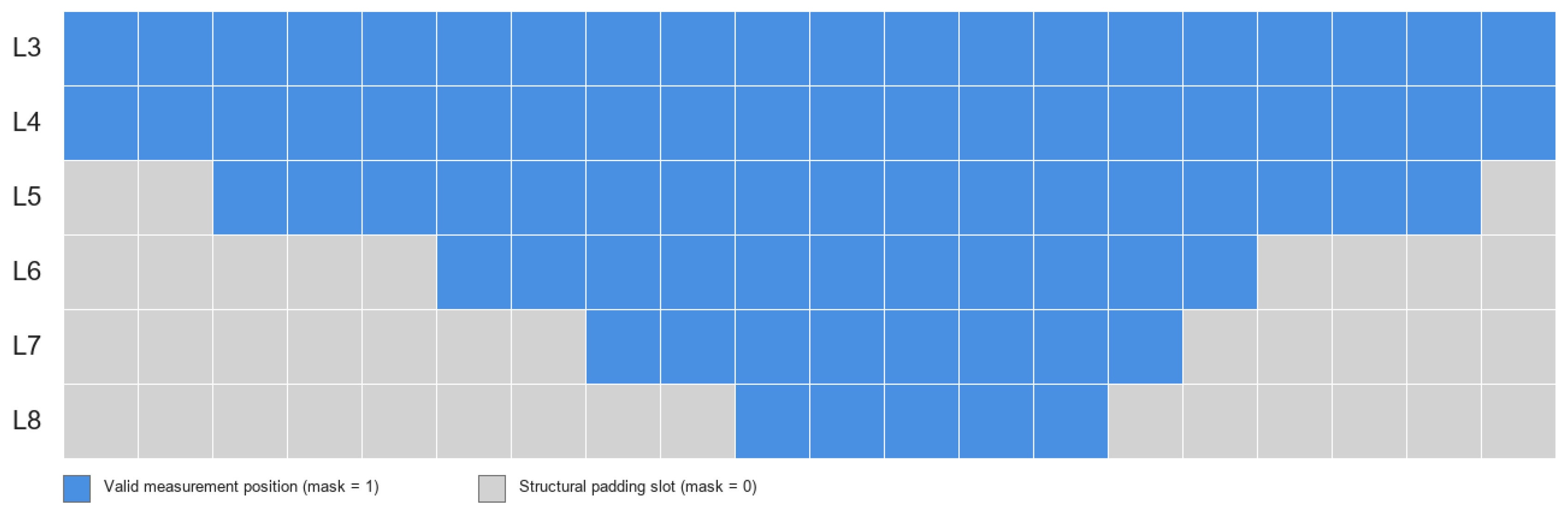
Six collimation survey lines, from L3 to L8, were used in the analysis. The original engineering network contained 89 monitoring points arranged along the dam-axis direction and at different elevations of the dam body. After data screening, spatial alignment, and consistency checking for long-term reconstruction, 81 positions were retained as valid modeling and evaluation locations in the unified field representation, while the remaining points were not used as forecast targets in the present study. This distinction is important because the reconstructed field is defined for modeling consistency and does not imply that all original engineering points were retained as valid positions in the final learning object. The retained positions cover the dam crest, downstream slope, and other key deformation observation areas, allowing the monitoring system to describe both temporal changes and spatial differences in dam displacement.

Each monitoring point contains three displacement components, corresponding to the dam-axis direction, the downstream river direction, and the vertical direction. In this study, these components are denoted as X, Y, and Z, respectively. To ensure consistency in modeling and interpretation, the displacement sign convention follows the original engineering data definition. The positive X direction is defined along the positive dam-axis direction, the positive Y direction is defined downstream along the river direction, and the positive Z direction follows the vertical displacement convention used in the original monitoring records.

2.2. Monitoring Variables, Temporal Coverage, and Data Characteristics

The dataset used in this study contains three categories of information: multi-point dam displacement, environmental and operational variables, and data-availability indicators. Displacement observations were obtained from 81 retained monitoring positions distributed across six survey lines, L3–L8. At each position, the X component denotes relative displacement along the positive dam-axis direction, the Y component denotes relative horizontal displacement toward the downstream direction, and the Z component denotes relative vertical displacement according to the sign convention adopted in the original monitoring system. The three displacement components are expressed in millimetres and are used both as historical input variables and as forecasting targets.

The original environmental variables consist of air temperature, reservoir water level, and rainfall. Air temperature is expressed in degrees Celsius, reservoir water level in metres, and rainfall in millimetres over the corresponding daily interval. To represent environmental effects over different temporal scales, six causal rolling variables were constructed: the 7-day and 30-day moving averages of air temperature, the 7-day and 30-day moving averages of reservoir water level, and the 7-day and 30-day cumulative rainfall. Each rolling variable was calculated using only the current and preceding observations, without using information from future dates.

Four calendar variables were additionally introduced to represent annual and monthly periodicity, including the sine and cosine encodings of the day of year and the sine and cosine encodings of the month. These variables are dimensionless. A static valid-position mask was used to distinguish the 81 retained monitoring positions from the 39 structural padding positions on the unified 6 × 20 spatial canvas. A separate dynamic observation-status variable indicated whether the displacement value at a valid position on a particular day was directly measured or obtained through causal forward filling.

The original displacement measurements were collected at nonuniform intervals according to the engineering survey schedule, whereas the environmental records were organized as daily series. For model construction, all variables were aligned to a common daily calendar from 2 June 2007 to 10 October 2025, corresponding to 6706 calendar days. The complete raw displacement-monitoring campaign extends from 5 January 2001 to 10 October 2025. However, the common model-ready period used for forecasting begins on 2 June 2007, when the retained displacement, environmental, and operational variables provide joint temporal coverage on the daily grid. All reported observation-availability and forward-filling statistics in this study are therefore defined on this common 6706-day model-ready period rather than on the full raw monitoring campaign. The modeling interval was therefore one day. When an observation was unavailable, the most recently available historical value was carried forward, and the corresponding observation-status indicator was set to zero. No backward filling or interpolation using future observations was employed.

Each daily input object contained 18 channels: three displacement channels, three original environmental and operational channels, six causally derived rolling channels, four calendar-encoding channels, one static valid-position-mask channel, and one dynamic observation-status channel. The prediction target consisted of the X-, Y-, and Z-direction displacement values at the 81 valid monitoring positions over the subsequent 60 days.

Table 1. Physical meaning, unit, temporal resolution, and modeling role of the variables used in the study.

Category	Variable	Physical Meaning	Unit	Temporal Resolution	Modeling Role
Multi-point displacement	X displacement	Relative displacement along the positive dam-axis direction	mm	Irregular survey observations aligned to the daily timeline	Historical input and forecasting target
Multi-point displacement	Y displacement	Relative horizontal displacement toward the downstream direction	mm	Irregular survey observations aligned to the daily timeline	Historical input and forecasting target
Multi-point displacement	Z displacement	Relative vertical displacement according to the sign convention of the original monitoring system	mm	Irregular survey observations aligned to the daily timeline	Historical input and forecasting target
Environmental variable	Air temperature	Recorded air temperature at the dam site	°C	Daily	Input
Operational variable	Reservoir water level	Reservoir operating water level	m	Daily	Input
Environmental variable	Rainfall	Precipitation accumulated over the corresponding daily interval	mm	Daily	Input
Causal rolling variable	7-day mean air temperature	Mean air temperature over the current day and the preceding 6 days	°C	Daily derived variable	Input
Causal rolling variable	30-day mean air temperature	Mean air temperature over the current day and the preceding 29 days	°C	Daily derived variable	Input
Causal rolling variable	7-day mean reservoir water level	Mean reservoir water level over the current day and the preceding 6 days	m	Daily derived variable	Input
Causal rolling variable	30-day mean reservoir water level	Mean reservoir water level over the current day and the preceding 29 days	m	Daily derived variable	Input
Causal rolling variable	7-day cumulative rainfall	Rainfall accumulated over the current day and the preceding 6 days	mm	Daily derived variable	Input
Causal rolling variable	30-day cumulative rainfall	Rainfall accumulated over the current day and the preceding 29 days	mm	Daily derived variable	Input
Calendar encoding	Day-of-year sine	Sine encoding of the position within the annual cycle	Dimensionless	Daily derived variable	Input
Calendar encoding	Day-of-year cosine	Cosine encoding of the position within the annual cycle	Dimensionless	Daily derived variable	Input
Calendar encoding	Month sine	Sine encoding of the position within the month-of-year cycle	Dimensionless	Daily derived variable	Input
Calendar encoding	Month cosine	Cosine encoding of the position within the month-of-year cycle	Dimensionless	Daily derived variable	Input
Mask variable	Valid-position mask	Binary indicator distinguishing the 81 retained monitoring positions from the 39 structural padding positions on the unified 6 × 20 spatial canvas	Binary (0/1)	Static	Input; defines the official loss and evaluation boundary
Data-availability indicator	Observation-status indicator	Binary indicator specifying whether a displacement value at a valid position was directly observed or obtained through causal forward filling	Binary (0/1)	Daily	Input

Note: The rolling variables were calculated causally using only the current and preceding observations. For the valid-position mask, 1 denotes a retained monitoring position and 0 denotes a structural padding position. For the observation-status indicator, 1 denotes a directly observed displacement value and 0 denotes a value obtained through causal forward filling.

summarizes the physical meaning, unit, temporal resolution, and modeling role of all variables.

Descriptive statistics were calculated using the original physical values before normalization. Structural padding positions were excluded from the displacement statistics. For the three displacement components, the statistics were calculated by pooling displacement values over all retained monitoring positions.

Table 2. Descriptive statistics and observation availability of the main continuous variables before normalization.

Variable Group	Variable	Unit	Directly Observed Values, Nobs	Direct-Observation Ratio Before Forward Filling (%)	Min	Max	Mean	Std.
Panel A. Original measured variables
Displacement	X displacement	mm	16,304	3	−195.24	135.52	−6.53	41.54
Displacement	Y displacement	mm	16,304	3	−355.58	446.37	119.01	102.42
Displacement	Z displacement	mm	16,304	3	−10.52	837.07	190.71	203.82
Environmental variable	Air temperature	°C	6546	97.61	−5.48	99.26	20.65	7.39
Operational variable	Reservoir water level	m	6648	99.14	732.85	780	758.78	12.46
Environmental variable	Rainfall	mm	2889	43.08	0	149	6.52	11.47
Panel B. Causally derived continuous variables
Causal rolling variable	7-day mean air temperature	°C	—	—	3.53	94.73	20.65	7.03
Causal rolling variable	30-day mean air temperature	°C	—	—	4.87	90.78	20.66	6.4
Causal rolling variable	7-day mean reservoir water level	m	—	—	733.14	779.97	758.76	12.44
Causal rolling variable	30-day mean reservoir water level	m	—	—	734.33	779.86	758.7	12.26
Causal rolling variable	7-day cumulative rainfall	mm	—	—	0	537	45.58	54.81
Causal rolling variable	30-day cumulative rainfall	mm	—	—	0.00	934.00	194.89	168.83

Note: Observation counts and direct-observation ratios are reported only for the original measured variables. The direct-observation ratio denotes the proportion of directly recorded values on the common model-ready daily grid before causal forward filling. For the displacement components, the denominator comprises all valid position–day combinations over the 81 retained monitoring positions and 6706 calendar days, while the 39 structural padding positions are excluded. For air temperature, reservoir water level, and rainfall, the denominator comprises the 6706 calendar days in the common model-ready period. Observation counts and direct-observation ratios are not separately reported for the causally derived rolling variables because these variables were constructed from the causally aligned daily series rather than directly measured. The minimum, maximum, mean, and standard deviation were calculated from the model-ready series in physical units after daily alignment and causal forward filling but before normalization.

summarizes the descriptive statistics and observation availability of the main continuous variables before normalization. Observation counts and direct-observation ratios are reported for the original measured variables before causal forward filling, whereas the minimum, maximum, mean, and standard deviation are reported for both the original measured variables and the causally derived rolling variables using the model-ready series. These descriptive statistics are provided only for data characterization, whereas all normalization parameters were estimated exclusively from the training subset.

Across all valid position–day combinations during the common model-ready period, 3.00% contained directly observed displacement values, whereas 97.00% were populated through causal forward filling. Observation availability was also quantified separately for survey lines L3–L8. The direct-observation ratios for L3–L8 were 3.19%, 3.18%, 2.16%, 3.32%, 3.28%, and 3.27%, respectively, with corresponding forward-filled proportions of 96.81%, 96.82%, 97.84%, 96.68%, 96.72%, and 96.73%. Observation availability was therefore not spatially uniform across the monitoring network. In particular, L5 had the lowest direct-observation ratio and the highest reliance on causal forward filling under the present daily grid reconstruction.

2.3. Field-Oriented Digital Representation of Monitoring Records

In this study, the reconstructed displacement field is treated as a unified engineering data object rather than a simple reshaped array.

The original monitoring data are not treated as a collection of isolated point-wise time series. For dam deformation monitoring, the spatial arrangement of survey lines and monitoring points contains important engineering information. Points on the same survey line describe deformation changes along a similar elevation or structural zone, while points from different survey lines reflect vertical distribution and deformation differences across the dam body. Therefore, this study organizes monitoring records as discrete samples of a dam displacement field rather than independent monitoring sequences.

For each observation day, displacement values from survey lines L3 to L8 are mapped into a two-dimensional spatial matrix. The row index corresponds to the survey line, and the column index corresponds to the monitoring point order along that line. The three displacement directions are stored as separate channels. In this way, the displacement field at time step t is written as

$$X_t\in {ℝ}^{H\times W\times C}$$

(1)

where H is the number of survey lines, W is the maximum number of monitoring point positions among the selected survey lines, and C is the number of displacement components. In this study, H = 6 and C = 3. The three channels correspond to the X, Y, and Z displacement components.

By stacking the daily displacement fields along the time axis, the full monitoring sequence can be expressed as

$$X_{1:T}=\left\{X_1,X_2,\dots ,X_T\right\}$$

(2)

where T denotes the number of daily time steps after preprocessing. This representation preserves the survey-line structure of the monitoring system and transforms long-term deformation records into a field-oriented spatiotemporal forecasting object. It also provides a common database for comparing different types of forecasting models.

It should be noted that adjacency in the reconstructed 6 × 20 field does not represent a strict geometric neighborhood in the sense of a regular physical mesh. The row dimension follows the ordered survey lines from L3 to L8 and therefore preserves the survey-line-level and elevation-related organization of the monitoring system. The column dimension follows the aligned monitoring-point order within each survey line, so neighboring columns primarily indicate ordinal proximity along the same engineering line rather than equal physical spacing, identical elevation, or one-to-one structural equivalence across different lines. Accordingly, the reconstructed field should be interpreted as an ordered engineering representation with constrained physical meaning: it preserves survey-line membership, within-line positional order, and the broad structural organization of the monitoring system, but it does not encode exact Euclidean adjacency or a complete geometric representation of the dam body.

2.4. Definition of Valid-Position Mask for Unequal Monitoring Layouts

A practical difficulty in reconstructing multi-line monitoring data is that different survey lines contain different numbers of monitoring points. Directly forcing all survey lines into a fixed-size matrix introduces padded positions that do not correspond to real observations. If these padded positions are treated in the same way as valid measurements, they may affect both model training and error evaluation.

To address this problem, a valid-position mask is introduced together with the displacement-field tensor. The mask is defined as

$$\mathit{M}\in {\left\{0,1\right\}}^{H\times W}$$

(3)

where M_h,w = 1 indicates that the position (h,w) corresponds to a real monitoring point, and M_h,w = 0 indicates a padded position. The same mask is shared by the X-, Y-, and Z-direction displacement channels because the spatial layout is determined by the survey-line arrangement. In the reconstructed field, the fixed spatial canvas contains H × W = 6 × 20 = 120 positions. Among them, 81 positions correspond to retained valid monitoring locations used for model training and official evaluation, whereas the remaining 39 positions are structural placeholders introduced to keep a consistent matrix form across survey lines with unequal numbers of monitored points. These padded positions are part of the digital representation for computational consistency, but they do not correspond to actual forecast targets in the present study. The corresponding mask layout is shown in Figure 2.

During model training and evaluation, losses and errors are calculated only at valid monitoring positions. For example, the masked mean squared error can be written as

$${\mathrm{MSE}}_{mask}={\displaystyle \frac{{\displaystyle {\sum }_{t=1}^Q{\displaystyle {\sum }_{h=1}^H{\displaystyle {\sum }_{w=1}^W{\displaystyle {\sum }_{c=1}^C{M}_{h,w}}}}}{\left({\widehat{Y}}_{t,h,w,c}-Y_{t,h,w,c}\right)}^2}{QC{\displaystyle {\sum }_{h=1}^H{\displaystyle {\sum }_{w=1}^W{M}_{h,w}}}}},$$

(4)

where Y_t,h,w,c and ${\widehat{Y}}_{t,h,w,c}$ denote the observed and predicted displacement values, respectively, and Q is the forecasting horizon; H and W define the spatial matrix size; and C is the number of displacement channels. Here, H = 6, W = 20, C = 3, with the three channels corresponding to the X-, Y-, and Z-direction displacements. The mask prevents padded positions from contributing to the loss and keeps the evaluation restricted to real monitoring points. Its effect on forecasting performance is model-dependent, which is examined further in Section 4.3.

In implementation, the valid-position mask is a static two-dimensional binary matrix defined on the common 6 × 20 spatial canvas and shared by all samples. During loss calculation, the mask is broadcast across the forecasting-horizon and displacement-channel dimensions so that only valid position–horizon–channel combinations contribute to the official objective. For PatchTST and TimesNet, the internal predictions are first restored from the flattened temporal representation to the common 60 × 6 × 20 × 3 future displacement-field layout before the mask is applied. The same valid-position boundary is used consistently for training loss, validation loss, checkpoint selection, and test-set evaluation. The dynamic observation-status channel is used only as input metadata to distinguish directly observed values from causally forward-filled values and does not modify the static valid-position boundary.

The same field-oriented representation is used for all four forecasting models. SimVP and SimVPv2 operate directly on the reconstructed two-dimensional field, whereas PatchTST and TimesNet use multivariate temporal inputs adapted from the same field-oriented representation through full-field flattening. The model outputs are then mapped back to the original field layout for comparison.

2.5. Data Preprocessing and Supervised Sample Construction

Several preprocessing steps were applied before supervised samples were generated. First, the displacement baseline was unified to avoid systematic offsets among different survey lines. Historical monitoring records may use different reference dates or engineering baselines. In this study, the selected records were converted into a consistent displacement representation before model training, while the original baseline information was retained for traceability rather than used as a model input.

Second, missing observations were processed using a causal forward-fill strategy to obtain continuous daily sequences without introducing future information. After alignment to the common daily timeline, both the displacement series and the environmental series were propagated forward using only previously available observations; backward filling and full-sequence interpolation were not used in the present rerun. This design ensured that the reconstructed daily inputs remained consistent with the chronological forecasting setting.

Third, normalization was applied channel by channel. The normalization parameters were computed using only the training subset and were then applied to the validation and test subsets. Environmental variables were standardized using the mean and standard deviation of the training subset, whereas displacement values were scaled to [0, 1] using the minimum and maximum values estimated from valid monitoring positions in the training subset. After prediction, the outputs were transformed back to the original displacement scale for error calculation and engineering interpretation.

The supervised forecasting samples were generated using a sliding-window strategy. A historical sequence of 120 consecutive days was used as the input, and the following 60 days were used as the prediction target. For the i-th sample, the input and output are written as

$${\mathbf{S}}_i^{in}=X_{i:i+119}$$

(5)

$${\mathbf{S}}_i^{out}=X_{i+120:i+179}$$

(6)

Thus, the model learns the mapping from historical displacement fields to future displacement fields:

$$f_{\theta }:{ℝ}^{120\times H\times W\times C}\to {ℝ}^{60\times H\times W\times C}$$

(7)

The sliding window moved along the full monitoring sequence with a stride of one day. The generated samples were divided into training, validation, and test sets in chronological order. Random shuffling was not used because the forecasting task should reflect the engineering situation in which future displacement is predicted only from past monitoring records.

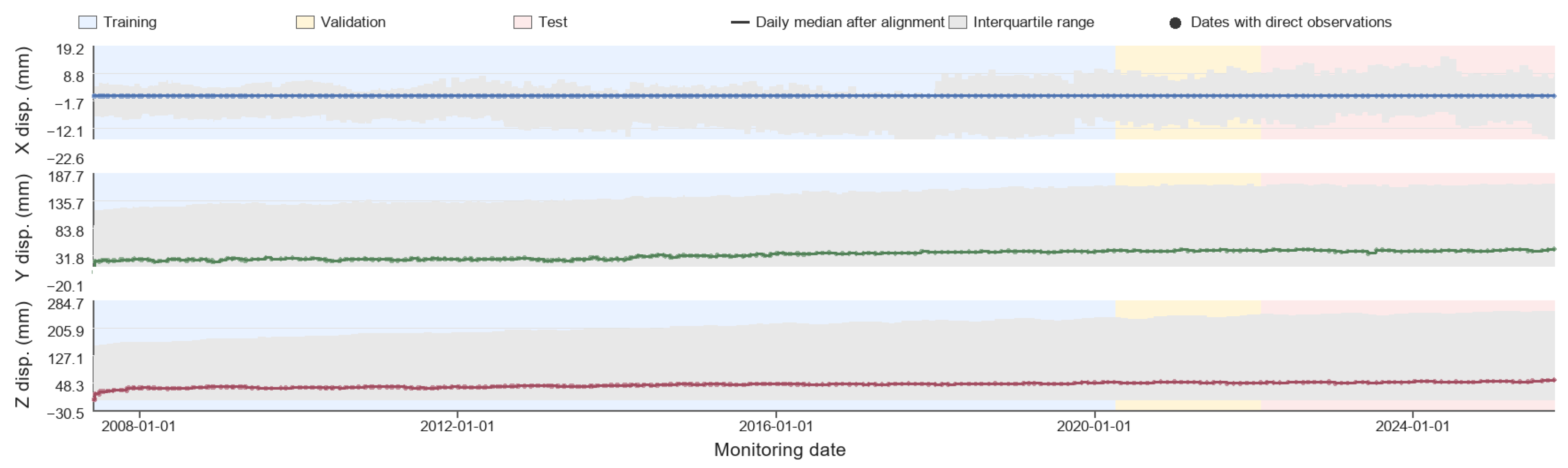
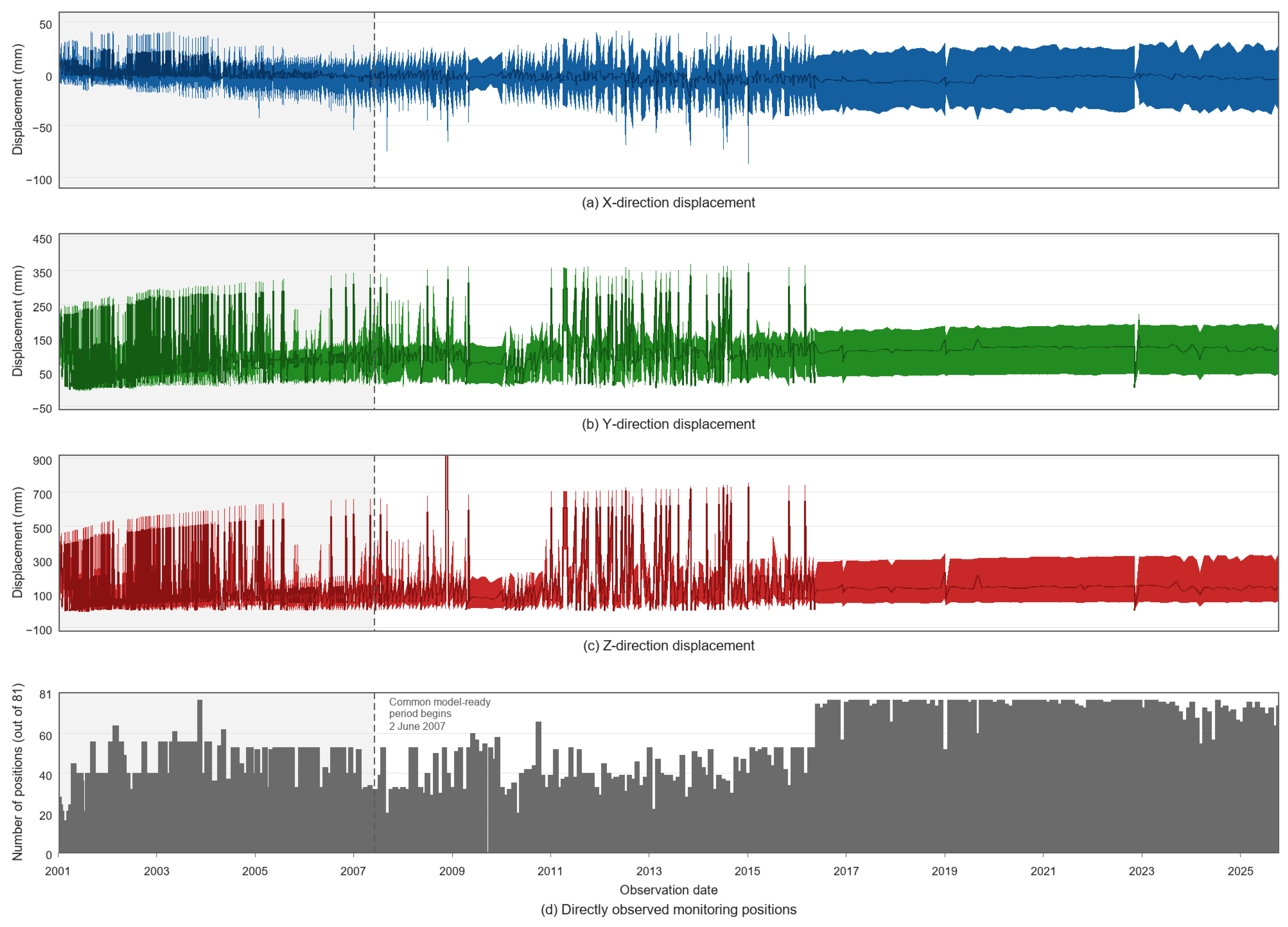
Figure 3 presents the long-term evolution of the reconstructed displacement records and the chronological division of the dataset. For each displacement component, the solid line represents the median value across the retained valid monitoring positions, while the shaded band denotes the corresponding interquartile range from the 25th to the 75th percentile. The background colors indicate the training, validation, and test periods. The figure shows that the three displacement components exhibit different long-term evolution patterns and spatial dispersion characteristics. The chronological split preserves the temporal order of the monitoring records and ensures that the test subset represents a later operational stage that is not used during model training.

The X-direction median remains relatively stable over the monitoring period, whereas the interquartile range varies over time, indicating that local point-wise differences cannot be fully represented by the global median trend alone.

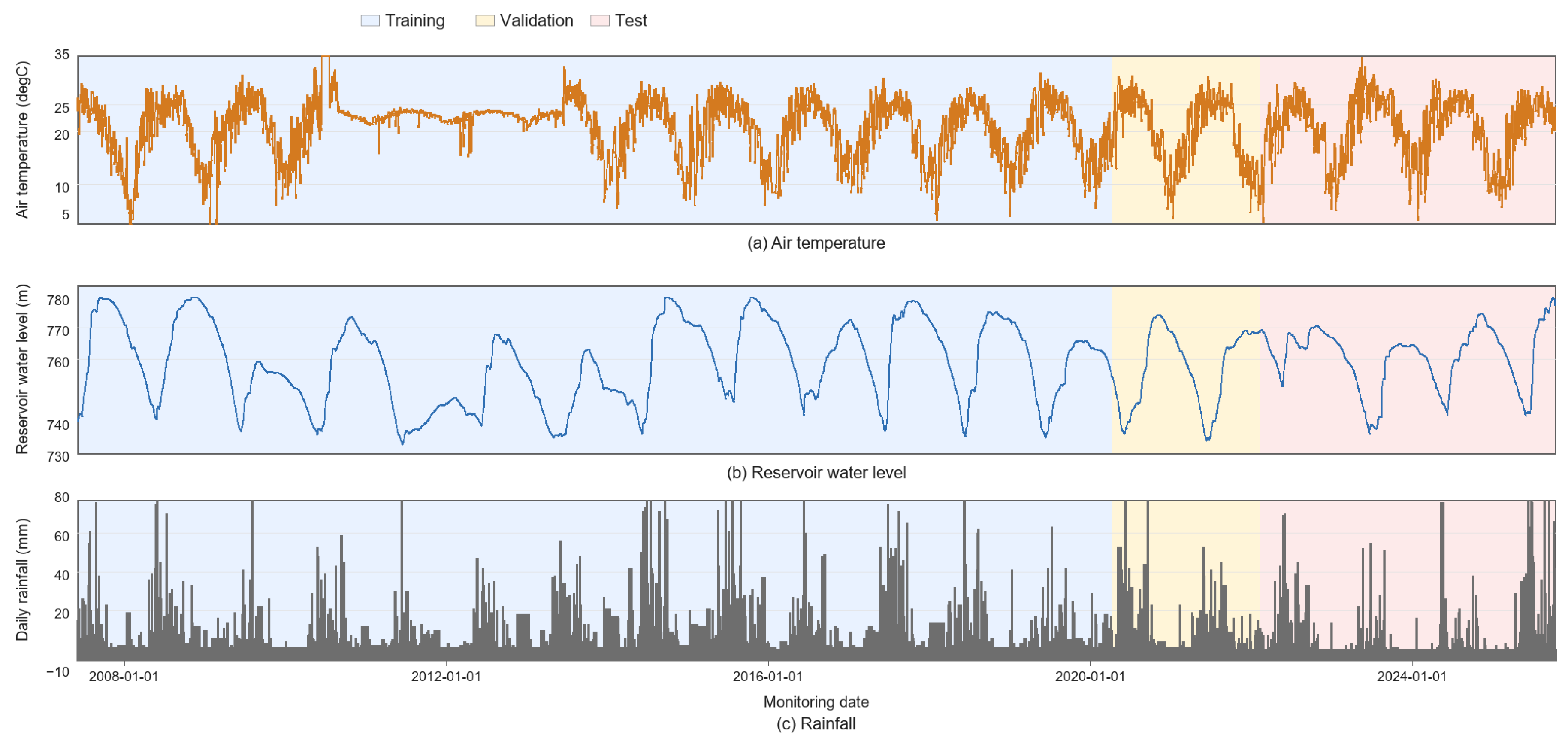
To complement the displacement evolution shown in Figure 3, Figure 4 presents the temporal evolution of the main environmental and operational variables used in the forecasting task, including air temperature, reservoir water level, and daily rainfall. The background shading indicates chronological training, validation, and test periods. These variables exhibit different temporal characteristics: air temperature shows pronounced seasonal fluctuations, reservoir water level reflects cyclic and stage-dependent operating conditions, and rainfall is intermittent with concentrated high-intensity events.

The temporal patterns shown in Figure 4 confirm that the forecasting period covers multiple seasonal cycles and substantially different reservoir operating and rainfall conditions. The chronological split retains these temporal characteristics while ensuring that the validation and test periods correspond to later operational stages that were not used for model training. The environmental and operational variables were incorporated not only in their original daily forms but also through causally derived 7-day and 30-day rolling features to represent responses over different temporal scales.

To further characterize the original acquisition pattern of the displacement records, Figure 5 presents the temporal evolution and observation coverage of the directly observed X-, Y-, and Z-direction displacements. For each survey date, the upper three panels summarize the directly observed displacement values across the available monitoring positions, while the bottom panel shows the number of monitoring positions with direct observations. While the observation-availability ratios reported in Section 2.2 quantify the overall and survey-line-specific extent of causal forward filling on the common daily grid, Figure 5 illustrates the temporal variation in direct observation coverage during the monitoring campaign. The complete raw displacement-monitoring campaign extends from 5 January 2001 to 10 October 2025, whereas the common model-ready period begins on 2 June 2007, when the retained displacement, environmental, and operational records provide joint temporal coverage.

As shown in Figure 5, both the temporal spacing of the original survey records and the number of monitoring positions directly observed vary over the monitoring campaign. Observation coverage is relatively sparse and variable during several earlier periods, whereas a larger proportion of the 81 retained positions is generally available during the later monitoring stage. These characteristics support the use of a common daily timeline, causal forward filling, and the dynamic observation-status indicator. Because the set of directly observed positions is not identical on all survey dates, changes in the pooled median and interquartile range should be interpreted together with the observation-coverage panel and should not be attributed solely to changes in the overall structural response.

3. Unified Forecasting Framework and Model Adaptation

3.1. Framework for Unified Dual-Route Displacement Forecasting

Based on the field-oriented representation developed in Section 2, multi-point dam displacement prediction is formulated as a unified forecasting task. The purpose is not simply to compare several algorithms on the same dataset, but to examine how different modeling routes behave when they are applied to the same reconstructed monitoring object under the same physical monitoring definition.

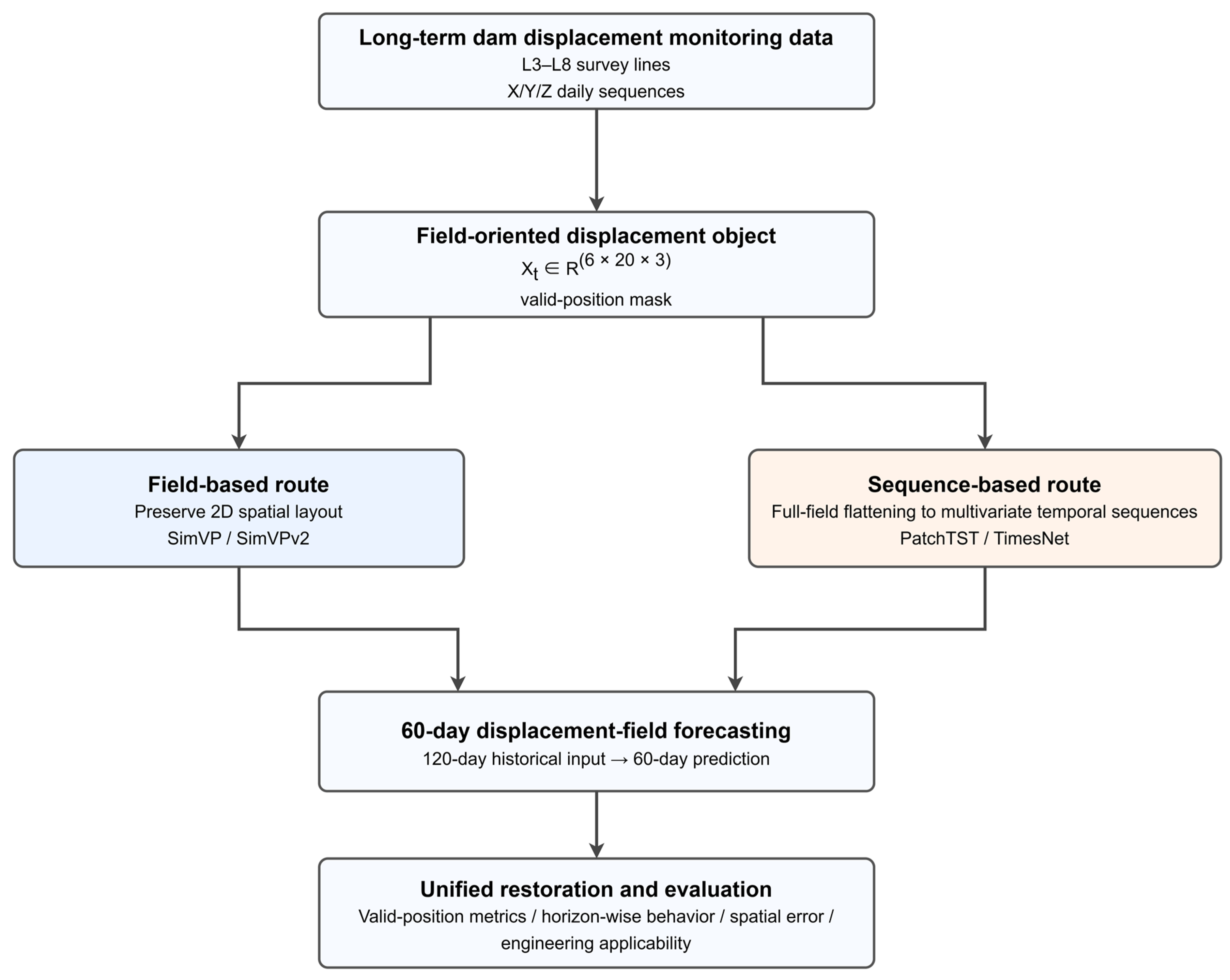
As shown in Figure 6, the long-term monitoring records are first organized according to the survey-line layout and the X-, Y-, and Z-direction displacement components. The reconstructed daily displacement field preserves the ordered arrangement of the monitoring positions. A valid-position-aware protocol is then used to distinguish actual measurement locations from the structural padding introduced by the unequal numbers of monitoring points across the six survey lines. In this way, padded entries remain part of the fixed matrix form required for unified modeling, but they are excluded from the official loss calculation and performance evaluation because they do not correspond to actual displacement observations.

Two forecasting routes are constructed from the same field-oriented displacement object. The field-based route, represented by SimVP and SimVPv2, directly preserves the reconstructed two-dimensional spatial layout during forecasting. The sequence-based route, represented by PatchTST and TimesNet, reorganizes the same unified field-oriented tensor into multivariate temporal sequences through full-field flattening. The distinction between the two routes therefore lies mainly in how the same physical monitoring object is represented during feature extraction and prediction, rather than in differences in data source, prediction target, or evaluation boundary.

The forecasting task is kept identical for all four models. Historical displacement records over 120 consecutive days are used to predict the displacement evolution over the following 60 days. The chronological data split, normalization procedure, valid-position loss and evaluation boundary, and official performance metrics remain unchanged across the experiments. After prediction, the outputs of both routes are restored to the original monitoring layout and evaluated at the same valid monitoring positions. This unified setting allows differences in forecasting performance to be interpreted mainly in terms of the modeling route rather than inconsistencies in data preparation.

The dual-route framework is also relevant to digital engineering practice. Long-term monitoring systems often require model replacement, periodic retraining, and continuous updating as new measurements become available. A common field-oriented displacement object provides a stable connection between the engineering monitoring layout and different forecasting models. It therefore supports not only route-level comparison of predictive behavior, but also the assessment of direction-wise differences, horizon-wise stability, spatial error distribution, and engineering applicability within a unified digital representation.

3.2. Adaptation of Field-Based and Sequence-Based Models

The four forecasting models considered in this study differ in how they represent and process monitoring data. To ensure a consistent comparison, all models start from the same unified field-oriented input object, while their inputs are adapted according to the native structure of each model. In the main experiments, the physical meaning of the monitoring positions, the valid-position loss and evaluation boundary, and the forecasting target remain unchanged throughout the adaptation process.

3.2.1. Field-Based Route

For SimVP and SimVPv2, the reconstructed field-oriented tensors are used directly as model inputs. The row dimension corresponds to survey lines L3–L8, and the column dimension represents the aligned monitoring-point positions along each line. The channel dimension contains the displacement, environmental, valid-position-mask, and observation-status information defined in Section 3.4. The prediction target contains the X-, Y-, and Z-direction displacement components only. Structural padding is retained to preserve the fixed matrix size, while the valid-position-aware protocol ensures that padded entries are excluded from the official loss calculation and performance evaluation.

This route explicitly preserves the two-dimensional organization of the monitoring network during forecasting. Proximity in the reconstructed field reflects the ordered engineering arrangement of survey lines and monitoring points rather than strict Euclidean adjacency. The field-based route should therefore be interpreted as exploiting survey-line membership, within-line positional order, and the local continuity implied by the monitoring arrangement, without assuming that every pair of neighboring matrix cells represents physically adjacent locations in the dam geometry. The field-based route is therefore used to examine how explicit preservation of the ordered monitoring layout affects multi-point displacement forecasting under the same physical monitoring definition.

3.2.2. Sequence-Based Route

For PatchTST and TimesNet, the same unified field-oriented input object is reused, but it is internally adapted into a multivariate temporal sequence for sequence modeling. In the current implementation, each sample first enters the framework as a 120 × 6 × 20 × 18 tensor, and the sequence-based models then flatten the spatial-canvas and channel dimensions into a daily multivariate representation before temporal feature extraction. Under this setting, the effective internal sequence input can be viewed as a 120 × 2160 multivariate series, while the prediction target remains defined on the unified 60 × 6 × 20 × 3 displacement field.

In this route, the two-dimensional engineering layout is no longer explicitly preserved during temporal modeling. Instead, the fixed variable ordering maintains a stable correspondence between each temporal variable and its original physical position after full-field flattening. Spatial relationships are therefore not encoded directly and can only be learned indirectly from statistical dependencies among the flattened variables.

Comparing this route with the field-based route helps clarify how different model families behave when they are applied to the same physical monitoring object under the same prediction task and evaluation boundary. In the subsequent restoration and evaluation stage, predictions are mapped back to the unified displacement-field form and evaluated at the same valid monitoring positions. When the monitoring configuration changes, sequence-based models may offer higher update flexibility, although feature-index remapping and model-specific input adaptation may still be required.

The model adaptations are summarized in

Table 3. Adaptation of the four forecasting models under the unified field-oriented engineering data object.

Model	Forecasting Route	Model Input	Treatment of Spatial Structure	Role in this Study
SimVP	Field-based route	Field-oriented spatiotemporal tensor defined on the unified 6 × 20 canvas	Explicitly retained through the reconstructed survey-line and monitoring-point layout	Compact field-based baseline
SimVPv2	Field-based route	Field-oriented spatiotemporal tensor defined on the unified 6 × 20 canvas	Explicitly retained through the reconstructed survey-line and monitoring-point layout	Enhanced field-based model
PatchTST	Sequence-based route	Multivariate temporal sequence adapted from the same unified tensor through full-field flattening	Not explicitly preserved during temporal modeling; stable physical correspondence retained through fixed variable ordering	Transformer-based temporal baseline
TimesNet	Sequence-based route	Multivariate temporal sequence adapted from the same unified tensor through full-field flattening	Not explicitly preserved during temporal modeling; stable physical correspondence retained through fixed variable ordering	General temporal-pattern baseline

.

3.3. Representative Forecasting Models and Non-Neural Baselines

Four trained forecasting models were implemented to compare field-based and sequence-based routes under the same field-oriented engineering data object. SimVP and SimVPv2 represent the field-based route and operate directly on the reconstructed spatiotemporal field tensor, retaining the ordered survey-line and monitoring-point layout during feature extraction. PatchTST and TimesNet represent the sequence-based route and use multivariate temporal inputs obtained from the same unified tensor through full-field flattening. Although their internal representations differ, all four trained models receive information derived from the same unified 120-day input object, generate the complete 60-day forecasting horizon, and restore their outputs to the common 60 × 6 × 20 × 3 displacement-field layout before valid-position-aware evaluation. In addition, a persistence baseline and a Holt damped-trend baseline were introduced to provide non-neural reference levels for the forecasting task under the same information boundary.

3.3.1. SimVP

SimVP is used as the compact representative model for the field-based route [13]. The model adopts an encoder–translator–decoder architecture built entirely with convolutional neural networks. The encoder extracts spatial features from the historical inputs, the translator models temporal evolution in the latent space, and the decoder reconstructs the future field sequence.

In the present implementation, SimVP directly receives the 120 × 6 × 20 × 18 field-oriented input tensor and generates a complete 60-day forecast in a single forward pass. The spatial encoder, temporal translator, and decoder use hid_S = 16, hid_T = 128, N_S = 2, N_T = 4, and N_D = 2. The model output is mapped to the common 60 × 6 × 20 × 3 displacement-field form before the valid-position-aware loss and evaluation procedures are applied. Its relatively compact architecture provides a direct reference for examining whether preservation of the reconstructed monitoring layout is sufficient for medium-term multi-point displacement forecasting.

3.3.2. SimVPv2

SimVPv2 is included as an enhanced model for the field-based route [14]. It simplifies the original SimVP architecture by replacing heavier U-Net-like components with plain convolutional stacks and introduces a Gated Spatiotemporal Attention mechanism to improve feature modeling. The model retains the ability to perform direct multi-step forecasting while providing an enhanced field-based architecture relative to SimVP.

In this study, SimVPv2 uses the same 120 × 6 × 20 × 18 field-oriented input tensor, the same 60 × 6 × 20 × 3 output definition, and the same valid-position-aware loss and evaluation boundary as SimVP. Its implementation uses hid_S = 16, hid_T = 128, N_S = 2, N_T = 4, and N_D = 2. The comparison between SimVP and SimVPv2 therefore isolates the effect of the enhanced field-based feature-transformation mechanism while keeping the monitoring representation, forecasting horizon, and physical evaluation boundary unchanged.

3.3.3. PatchTST

PatchTST is selected as the Transformer-based representative model for the sequence-based route [15]. It divides each historical time series into temporal patches and uses these patches as input tokens. This reduces the effective sequence length and allows the model to capture longer temporal dependencies more efficiently. PatchTST also adopts a channel-independent design, in which the same embedding and Transformer weights are shared across variables.

In the present framework, each sample first enters the unified data pipeline as a 120 × 6 × 20 × 18 tensor. The 6 × 20 spatial canvas and the 18 input channels are then flattened according to fixed position–channel ordering, producing a 120 × 2160 multivariate temporal input for PatchTST. The implementation uses a patch length of 4, a patch stride of 2, four attention heads, and a dropout rate of 0.1. The complete 60-day output is subsequently restored to the common 60 × 6 × 20 × 3 displacement-field layout before the valid-position mask is applied. Thus, the physical correspondence of each variable is preserved through fixed ordering, although the two-dimensional monitoring layout is not explicitly encoded during temporal modeling. Its performance therefore provides a useful reference for assessing how temporal modeling without explicit two-dimensional layout encoding can support multi-point dam displacement forecasting [17].

3.3.4. TimesNet

TimesNet is used as a general temporal-pattern representative model for the sequence-based route [16]. The model identifies multiple periodic patterns in a time series and transforms one-dimensional temporal variations into a set of two-dimensional tensors. The resulting representation allows intraperiod and interperiod variations to be modeled jointly through TimesBlock.

In this study, TimesNet uses the same 120 × 2160 multivariate temporal input as PatchTST, obtained by flattening the 6 × 20 spatial canvas and the 18 input channels according to the same fixed ordering. The implementation retains the three most prominent temporal periods through the top-k setting of k = 3. The model generates the complete 60-day forecast, after which its output is reshaped to the common 60 × 6 × 20 × 3 displacement-field layout. The same static valid-position mask is then used to define the official loss and evaluation boundary. Its inclusion provides a reference for assessing whether multi-period temporal modeling can capture the displacement evolution when the original two-dimensional survey-line layout is not explicitly retained.

3.3.5. Non-Neural Forecasting Baselines

Two non-neural reference baselines were introduced to provide reference levels for the forecasting task under the same information boundary. The persistence baseline repeats the displacement field available on the last day of the 120-day input window across the full 60-day forecasting horizon. The Holt damped-trend baseline independently fits a damped additive trend to each displacement component at each valid monitoring position using the same 120-day daily aligned and causally forward-filled input sequence. The level, trend, and damping parameters were estimated using the numerical optimization routine implemented in the forecasting library. Neither baseline used environmental or operational variables. Both baselines used only information available before the forecasting origin and were evaluated using the same test samples, forecasting horizons from t + 1 to t + 60, valid-position evaluation boundary, and evaluation metrics as the four trained models. The 39 structural padding positions were excluded from the evaluation.

3.4. Training Protocol

All four forecasting models were trained using the same supervised samples constructed from the long-term daily monitoring records. A unified field-oriented feature tensor was defined on a common 6 × 20 spatial canvas. For each day, the input tensor contained three displacement channels, thirteen environmental channels, one static valid-position mask channel, and one daily observation-status channel, giving 18 channels in total. The environmental channels comprised three original daily variables, namely air temperature, reservoir water level, and rainfall; six causal rolling features were derived from them, namely 7-day and 30-day temperature means, 7-day and 30-day water-level means, and 7-day and 30-day rainfall sums; and four calendar encodings were derived, namely day-of-year sine/cosine and month sine/cosine. The observation-status channel was defined point by point on the same 6 × 20 canvas, where a value of 1 indicated that the corresponding position had an actual observation on that day and a value of 0 indicated that the value at that position was carried forward after daily alignment. This dynamic channel was different from the static valid-position mask, which only distinguished retained monitoring locations from structural padding positions.

Each input sample therefore had a shape of 120 × 6 × 20 × 18, and each prediction target had a shape of 60 × 6 × 20 × 3.

The dataset was divided chronologically into training, validation, and test subsets using a nominal 70/10/20 split, without random shuffling across time. Under the causal forward-fill-only reconstruction used in the present rerun, the common daily timeline extended from 2 June 2007 to 10 October 2025. The training period covered 2 June 2007 to 7 April 2020, the validation period covered 8 April 2020 to 6 February 2022, and the test period covered 7 February 2022 to 10 October 2025. A one-day sliding window was used to generate supervised samples. For the training subset, the prediction horizon of each sample was constrained to fall entirely within the training period. For the validation and test subsets, the historical input window was allowed to extend into the immediately preceding period, while the prediction horizon remained entirely within the corresponding evaluation period. This preserved temporal continuity without introducing future-information leakage. The resulting dataset contained 4515 training samples, 611 validation samples, and 1283 test samples.

Normalization parameters were estimated from the training subset only. Environmental variables were standardized using the mean and standard deviation of the training subset, whereas displacement values were scaled to [0, 1] using the minimum and maximum values estimated from valid monitoring positions in the training subset. The same parameters were then applied to the validation and test subsets. After inference, all predictions were transformed back to the original displacement scale before error calculation.

The models were trained using Adam with an initial learning rate of 3 × 10⁻⁴, a batch size of 16, and a weight decay of 1 × 10⁻⁴. Smooth L1 loss with β = 0.02 was adopted during optimization. A five-epoch warmup followed by cosine decay was used for learning-rate scheduling, with the minimum learning rate set to 10% of the initial value. Each model was trained for 50 epochs, and the checkpoint with the lowest validation loss was selected for final evaluation.

During optimization, the training and validation losses were computed only at valid monitoring positions using the static valid-position mask, and the same boundary was retained for checkpoint selection and test-set evaluation. The dynamic observation-status channel was used only as input metadata and did not redefine the official loss or evaluation boundary. The influence of the mask setting is examined separately in Section 4.3. The common experimental settings are summarized in

Table 4. Common experimental settings of the four forecasting models.

Item	Common Setting
Spatial canvas	6 × 20
Input channels per day	18
Input window	120 days
Forecasting horizon	60 days
Sliding-window stride	1 day
Input sample shape	120 × 6 × 20 × 18
Prediction target shape	60 × 6 × 20 × 3
Train/validation/test split	Nominal 70/10/20 split; chronological order; no random shuffling
Optimizer	Adam
Initial learning rate	3 × 10−4
Batch size	Requested batch size: 16; runtime batch size adjusted when needed according to model and device memory
Weight decay	1 × 10−4
Loss function	Smooth L1 loss, β = 0.02
Learning-rate schedule	5-epoch warmup followed by cosine decay
Minimum learning rate	10% of the initial learning rate
Training epochs	50
Model selection criterion	Lowest validation loss
Loss/evaluation scope	Official loss and evaluation are computed on valid positions only

, while the model-specific architectural settings are listed in

Table 5. Main architecture-specific settings of the four forecasting models.

Model	Model-Specific Architectural Settings
SimVP	hidS = 16; hidT = 128; NS = 2; NT = 4; ND = 2
SimVPv2	hidS = 16; hidT = 128; NS = 2; NT = 4; ND = 2
PatchTST	Patch length: 4; patch stride: 2; number of heads: 4; dropout: 0.1
TimesNet	Top-k periods: 3

.

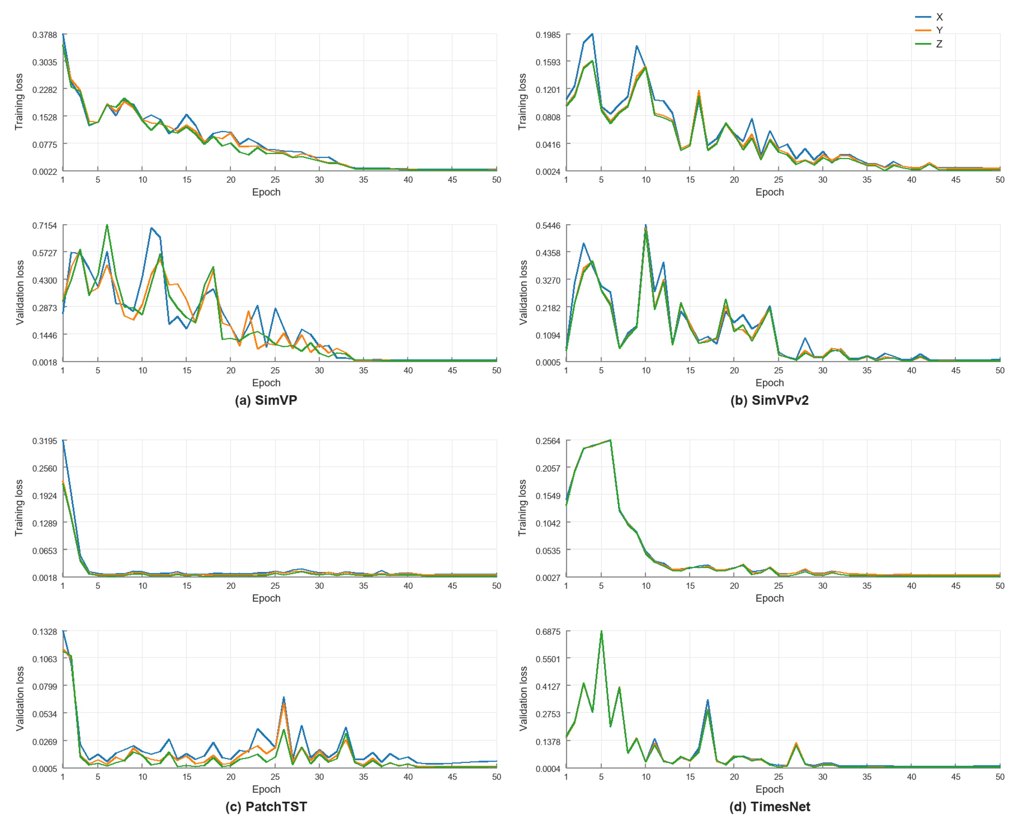
Figure 7 presents the combined training and validation loss curves of the four models.

Although the convergence patterns are not identical, the loss trajectories remain bounded and generally stabilize as training proceeds. SimVP and SimVPv2 show noticeable validation fluctuations during the early and intermediate stages, followed by more stable behavior in the later epochs. PatchTST converges rapidly during the initial stage and then remains at a relatively low loss level, although moderate fluctuations are still observed during the middle stage. TimesNet also exhibits noticeable early adjustments before reaching a relatively stable level in the later epochs. Overall, the four models show reasonable convergence behavior under the adopted training protocol, providing a consistent basis for the subsequent test-set comparison.

3.5. Engineering-Oriented Evaluation Strategy

The evaluation strategy was designed to assess not only predictive accuracy, but also the engineering usefulness of the proposed framework under the same physical monitoring definition. Unless otherwise stated, the official performance metrics were computed only at valid monitoring positions, whereas padded locations introduced during matrix reconstruction were excluded because they did not correspond to actual displacement observations.

The evaluation covered five complementary aspects. Overall test-set performance was compared using MSE, RMSE, MAE, and R² for the X-, Y-, and Z-direction displacement components, because the three directions have different physical meanings and may exhibit different temporal and spatial behaviors. Route-level horizon-wise errors were then examined at four representative forecasting horizons, namely t + 1, t + 7, t + 30, and t + 60. The field-based route was represented by the mean performance of SimVP and SimVPv2, whereas the sequence-based route was represented by the mean performance of PatchTST and TimesNet. Spatial error distributions were further analyzed by mapping the mean absolute error at each valid monitoring position back to the reconstructed displacement-field layout. The spatial MAE was averaged over the test samples and the same four representative forecasting horizons, so that local error concentrations and route-level spatial differences could be examined directly.

A validation-based ablation of the valid-position-aware loss boundary was also conducted under the same time-ordered split and the same main hyperparameter settings. The only factor that changed was whether the training and validation loss was computed over valid monitoring positions only or over all matrix positions, including structural padding entries. This analysis was intended to clarify the methodological role of the valid-position-aware protocol in defining a physically meaningful monitoring boundary, rather than to assume that it would necessarily improve every model. Engineering applicability was finally compared in terms of parameter scale, training-step time, single-sample inference latency, dependence on the two-dimensional monitoring layout, and ease of deployment and updating. The reported timing results were intended for relative comparison within the current computing environment rather than as absolute cross-platform benchmarks.

4. Forecasting Results and Route-Level Evaluation

4.1. Overall Forecasting Performance of the Four Models

The overall forecasting performance of the six models was evaluated on the held-out test set constructed from the daily monitoring series after causal forward-fill-only preprocessing. Under this reconstruction, the test period extended from 7 February 2022 to 10 October 2025. All metrics were computed only at valid monitoring positions under the valid-position-aware evaluation boundary. This evaluation setting ensured that the reported errors corresponded to actual monitoring locations rather than structural padding entries introduced during displacement-field reconstruction. The adopted metrics included MSE, RMSE, MAE, and R².

Table 6. Direction-wise forecasting performance of the two non-neural baselines and the four trained models on valid monitoring positions of the test set.

Direction	Model	MSE (mm2)	RMSE (mm)	MAE (mm)	R2
X	Persistence baseline	9.4	3.1	1.5	0.9958
	Holt damped trend	9.5	3.1	1.5	0.9958
	SimVP	9.4	3.1	1.5	0.9958
	SimVPv2	9.8	3.1	1.6	0.9957
	PatchTST	9.6	3.1	1.6	0.9957
	TimesNet	9.7	3.1	1.6	0.9957
Y	Persistence baseline	99.4	10.0	1.7	0.9911
	Holt damped trend	99.4	10.0	1.7	0.9911
	SimVP	100.0	10.0	1.9	0.9911
	SimVPv2	100.4	10.0	2.0	0.9910
	PatchTST	100.9	10.0	2.2	0.9910
	TimesNet	100.8	10.0	2.1	0.9910
Z	Persistence baseline	3.4	1.8	1.0	0.9999
	Holt damped trend	3.4	1.8	1.0	0.9999
	SimVP	2.9	1.7	1.0	0.9999
	SimVPv2	2.8	1.7	1.0	0.9999
	PatchTST	2.8	1.7	1.0	0.9999
	TimesNet	3.1	1.8	1.1	0.9999

summarizes the direction-wise prediction results of SimVP, SimVPv2, PatchTST, and TimesNet on this held-out test set.

To provide a fair comparison with the persistence and Holt damped-trend baselines, the four forecasting architectures were additionally rerun using a residual-anchor formulation. In this comparison setting, each model predicted the future displacement residual relative to the last model-ready displacement field in the 120-day input window. The predicted residuals were independently inverse-transformed to the original physical units and then added to the corresponding anchor field to reconstruct the absolute displacement forecasts. All six methods were evaluated using the same test samples, forecasting horizons, valid-position boundary, and physical-unit error metrics.

All methods were evaluated using the same held-out test samples, forecasting horizons from t + 1 to t + 60, and the same 81 retained monitoring positions. The 39 structural padding positions were excluded from the evaluation. For the four trained models, the forecasting targets were defined as future displacement residuals relative to the last displacement field in the input window. The predicted residuals were added to the last input state to reconstruct the absolute displacement fields before calculating the evaluation metrics. Lower MSE, RMSE, and MAE values indicate better performance, whereas higher R² values indicate closer agreement with the observed displacements. Bold values identify the best results based on unrounded numerical values.

As shown in Table 6, all six methods achieved high goodness-of-fit values, with $R^2$ values of approximately 0.996 in the X direction, 0.991 in the Y direction, and 0.9999 in the Z direction. However, the relative performance of the trained models and the two non-neural baselines varied across displacement directions and evaluation metrics.

In the X direction, all six methods produced essentially comparable results under the present case-specific setting. All RMSE values were 3.1 mm at the reported precision, while the MAE values ranged from 1.5 to 1.6 mm. The persistence baseline, Holt damped-trend baseline, and SimVP also yielded similar MSE values of approximately 9.4–9.5 mm². These differences are smaller than the adopted reporting precision and should not be interpreted as practically meaningful evidence that any individual method is generally more suitable for X-direction displacement forecasting.

In the Y direction, all methods obtained an RMSE of 10.0 mm at the reported precision, with R² values ranging from 0.9910 to 0.9911. The two non-neural baselines achieved lower MAE values of 1.7 mm, whereas the trained models produced MAE values ranging from 1.9 to 2.2 mm. Thus, under the present dam case and evaluation setting, the trained models did not demonstrate a consistent numerical advantage in the Y direction, despite exhibiting comparable squared-error-based performance.

In the Z direction, several trained models achieved lower squared-error-based metrics than the two non-neural baselines under the current experimental setting. SimVP, SimVPv2, and PatchTST yielded an RMSE of 1.7 mm, compared with 1.8 mm for the persistence and Holt damped-trend baselines, while their MSE values were approximately 2.8–2.9 mm², compared with 3.4 mm² for the baselines. TimesNet obtained a lower MSE than the baselines but the same reported RMSE of 1.8 mm. The MAE values remained close to 1.0 mm for most methods. These observations indicate a case-specific improvement in Z-direction squared-error-based metrics, but they do not establish that the corresponding architectures are generally more suitable for vertical displacement forecasting.

Overall, the four trained models did not exhibit universal superiority over the persistence and Holt damped-trend baselines. Under the present single-dam and case-specific experimental setting, their performance was essentially comparable to the baselines in the X direction, comparable in RMSE but weaker in MAE in the Y direction, and moderately better in the Z-direction squared-error-based metrics. These findings should be interpreted as case-specific comparative evidence rather than as a general direction-specific model-selection rule. Beyond aggregate numerical accuracy, the trained models operate within the proposed field-oriented forecasting framework, which incorporates environmental and operational variables and supports joint forecasting and spatial reconstruction of multi-point displacement fields.

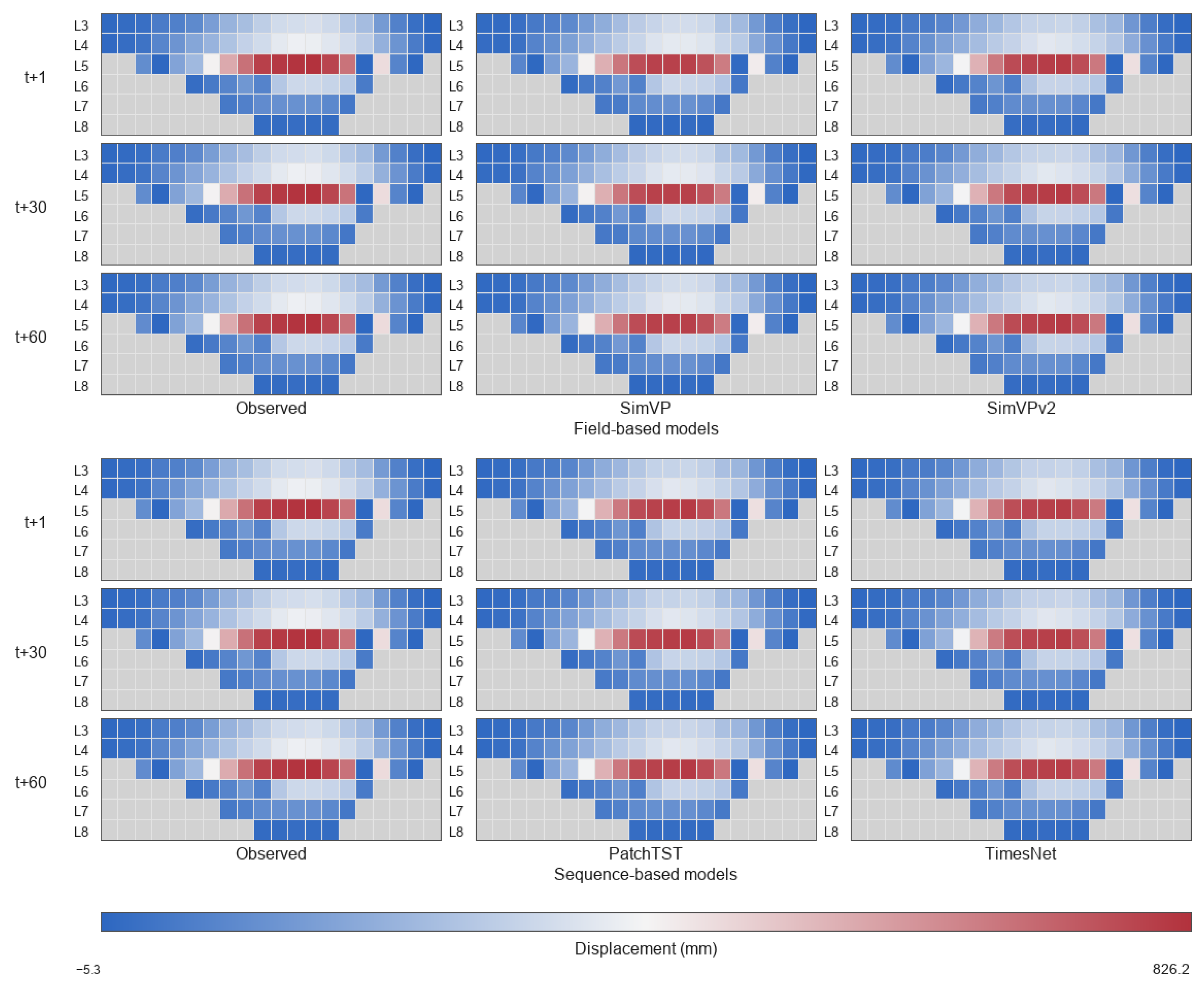
Figure 8 provides a qualitative illustration of the spatial reconstruction behavior of the four trained forecasting architectures under the route-comparison setting. It presents a representative comparison of the observed and predicted Z-direction displacement fields at t + 1, t + 30, and t + 60. The Z-direction component was selected because it exhibits the largest displacement magnitude and provides a clear visualization of the spatial deformation distribution. The selected case corresponds to a median-error sample under the SimVP test-set error ranking and is used to illustrate typical rather than best-case forecasting behavior. Gray cells denote structural padding positions excluded from the valid monitoring boundary. Accordingly, Figure 8 serves as a qualitative route-level illustration and is not used to support the residual-anchor baseline-comparison metrics reported in Table 6.

As shown in Figure 8, all four models reproduce the overall spatial pattern of the observed displacement field. In particular, the central high-displacement region and the surrounding lower-displacement zones remain identifiable across the three forecasting horizons. This similarity indicates that the predicted and observed fields exhibit broadly consistent spatial distributions rather than agreement only at isolated monitoring positions. The main discrepancies occur in the local displacement magnitude and the spatial extent of the central high-displacement region. These differences become more visible at longer forecasting horizons, particularly at t + 60, although the principal spatial organization of the observed field is still retained.

The quantitative results in Table 6 further show that forecasting performance should be interpreted jointly using absolute-error and goodness-of-fit metrics. In the X direction, all six methods achieved essentially comparable performance, with RMSE values of 3.1 mm and MAE values ranging from 1.5 to 1.6 mm. In the Y direction, all methods yielded an RMSE of 10.0 mm at the reported precision, although the persistence and Holt damped-trend baselines achieved lower MAE values of 1.7 mm than the four trained models, the MAE values of which ranged from 1.9 to 2.2 mm. In the Z direction, SimVP, SimVPv2, and PatchTST achieved lower RMSE values of 1.7 mm than the two non-neural baselines, which both yielded 1.8 mm. Their MSE values were also reduced from 3.4 mm² for the baselines to approximately 2.8–2.9 mm², whereas the MAE values remained generally close to 1.0 mm.

Overall, the four trained models did not exhibit universal superiority over the persistence and Holt damped-trend baselines across all displacement directions and evaluation metrics. Their performance was essentially comparable to the baselines in the X direction, comparable in RMSE but weaker in MAE in the Y direction, and moderately better in the Z-direction squared-error-based metrics. These results confirm the strong persistence of the monitored displacement series and indicate that forecasting effectiveness remains direction-dependent. Beyond aggregate numerical accuracy, the trained architectures operate within the proposed field-oriented framework, which integrates environmental and operational variables and supports joint multi-point forecasting and spatial reconstruction. The following analysis therefore focuses on the relative behavior of the field-based and sequence-based routes across forecasting horizons and displacement components.

4.2. Horizon-Wise Comparison of Field-Based and Sequence-Based Routes

To further evaluate the influence of the modeling route on multi-step displacement forecasting, the four models are grouped into two categories. The field-based route consists of SimVP and SimVPv2, which directly process the reconstructed displacement-field tensor. The sequence-based route consists of PatchTST and TimesNet, which reorganize the same unified displacement-field object into multivariate temporal sequences. For each route, the reported values represent the mean test-set performance of the two corresponding models. The comparison is conducted at four representative forecasting horizons: (t + 1), (t + 7), (t + 30), and (t + 60).

Table 7. Horizon-wise comparison between field-based and sequence-based forecasting routes.

Route	Horizon	MAE (mm)	RMSE (mm)	MAE-X (mm)	MAE-Y (mm)	MAE-Z (mm)	RMSE-X (mm)	RMSE-Y (mm)	RMSE-Z (mm)
Field-based	t + 1	6.0354	9.7518	4.6695	4.1522	9.2843	6.6467	9.3248	12.3960
Sequence-based	t + 1	6.1144	9.8495	4.6672	4.4010	9.2751	6.7064	9.8658	12.1952
Field-based	t + 7	6.0039	9.7406	4.6836	4.1880	9.1401	6.6449	9.4843	12.2562
Sequence-based	t + 7	6.1024	9.8219	4.6737	4.4180	9.2156	6.6787	9.8764	12.1347
Field-based	t + 30	5.9840	9.7733	4.7370	4.2469	8.9680	6.6387	9.8267	12.0727
Sequence-based	t + 30	6.0446	9.7267	4.6880	4.4917	8.9539	6.5803	9.9178	11.9220
Field-based	t + 60	5.8971	9.6492	4.7956	4.2395	8.6561	6.6185	9.8654	11.7456
Sequence-based	t + 60	5.9639	9.5931	4.7101	4.6280	8.5536	6.5086	10.0083	11.5554

presents the horizon-wise comparison between the two routes. The field-based route achieves slightly lower overall MAE values at all four forecasting horizons, with differences ranging from 0.0606 to 0.0985. The overall RMSE results are more balanced. The field-based route performs marginally better at t + 1 and t + 7, whereas the sequence-based route achieves slightly lower RMSE values at t + 30 and t + 60. The largest overall RMSE difference between the two routes is less than 0.10. Therefore, the present results do not indicate a systematic overall advantage for either forecasting route.

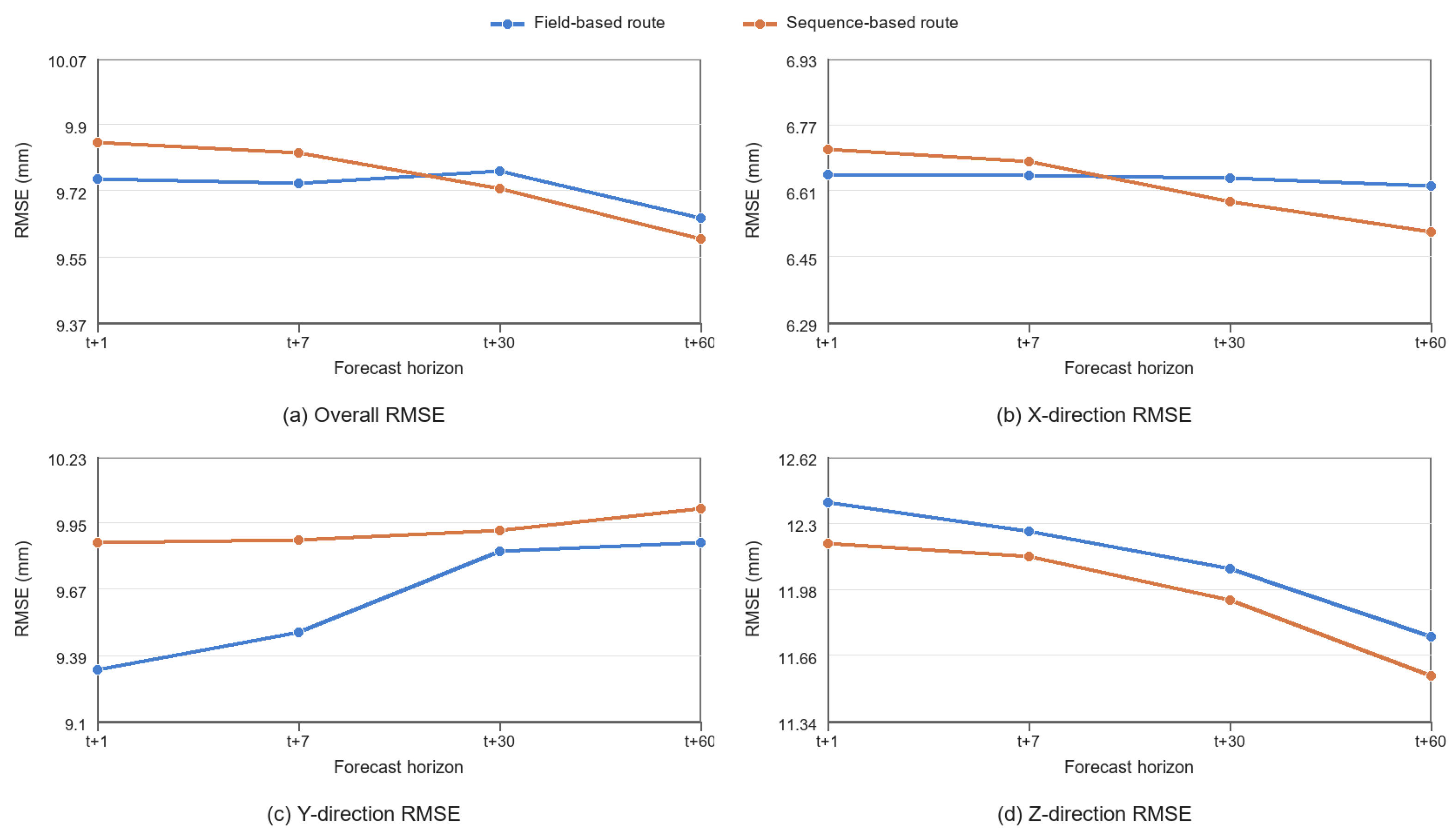
Figure 9 further visualizes the horizon-wise RMSE trends of the two forecasting routes, including the overall results and the direction-specific results for the X-, Y-, and Z-direction displacement components.

Figure 9 further visualizes the horizon-wise RMSE trends of the two forecasting routes. At each forecasting horizon, the RMSE of each model was calculated using prediction errors pooled over all test samples and valid monitoring positions, and the route-level value was obtained by averaging the RMSE values of the two constituent models. Panel (a) shows the overall route-level RMSE across the three displacement components, whereas panels (b–d) show the corresponding X-, Y-, and Z-direction RMSE values, respectively.

The direction-wise results reveal more specific route-level differences. For the Y-direction displacement, the field-based route consistently achieves lower RMSE values across all four representative horizons. The difference is most evident at t + 1, where the field-based and sequence-based routes obtain RMSE values of 9.3248 and 9.8658, respectively. This suggests that explicitly retaining the reconstructed monitoring layout may provide useful information for predicting the Y-direction displacement response under the present engineering setting.

For the Z-direction displacement, the sequence-based route shows slightly lower RMSE values across all four horizons. At t + 60, the corresponding RMSE values are 11.5554 and 11.7456 for the sequence-based and field-based routes, respectively. The X-direction results exhibit a horizon-dependent transition: the field-based route performs slightly better at t + 1 and t + 7, whereas the sequence-based route achieves lower RMSE values at t + 30 and t + 60.

Neither route exhibits evident progressive error amplification across the representative forecasting horizons. Overall, the results indicate that the influence of the modeling route depends on both the displacement component and the forecasting horizon. Explicit preservation of the reconstructed field layout may be beneficial for the Y-direction displacement, whereas sequence-based temporal modeling remains competitive for the Z-direction displacement and for longer-horizon X-direction forecasts. Rather than demonstrating the universal superiority of one route, the comparison highlights the importance of evaluating different forecasting models within the same physical monitoring definition and under a unified digital representation.

4.3. Ablation Analysis of Valid-Position Masking

The valid-position-aware protocol is introduced to handle the unequal numbers of monitoring points among different survey lines in the reconstructed displacement field. To examine its influence, a validation-based ablation experiment is conducted using the same time-ordered 70/10/20 dataset split and the same main hyperparameter settings as the main experiments. The only changed factor is the loss boundary: the training and validation loss is computed either on valid monitoring positions only or on all matrix positions, including structural padding entries.

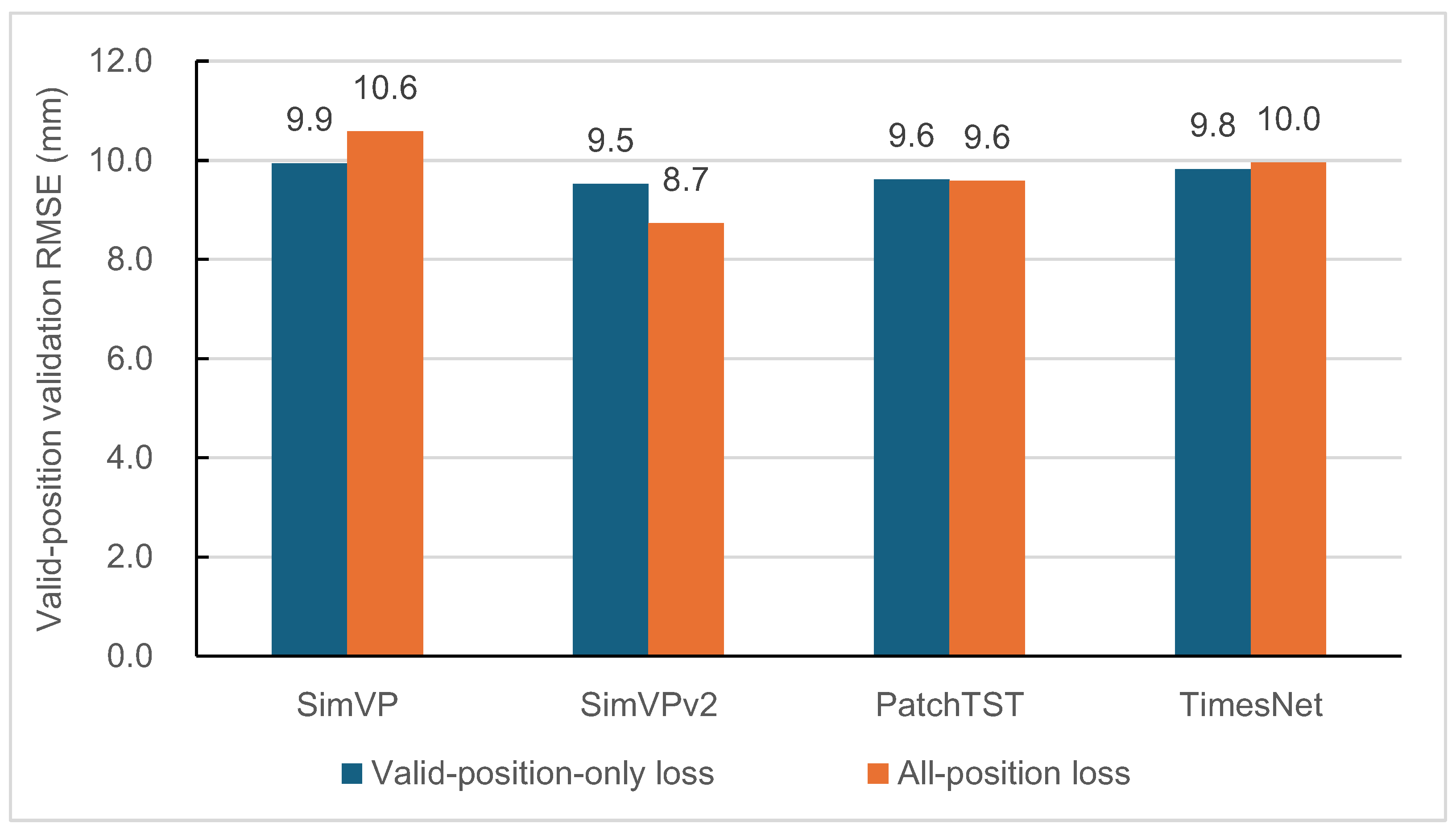
Figure 10 visualizes the valid-position validation RMSE obtained under these two loss-boundary settings. The mixed response across the four models indicates that extending the loss calculation to padded positions does not produce a uniform effect on validation accuracy.

For SimVP, extending the loss calculation from valid positions to all matrix positions increases the valid-position validation RMSE from 9.9 mm to 10.6 mm. For TimesNet, the same change also leads to a slight increase, from 9.8 mm to 10.0 mm. By contrast, SimVPv2 and PatchTST show lower valid-position validation RMSE values under the all-position loss setting, decreasing from 9.5 mm to 8.7 mm and from 9.6 mm to 9.6 mm, respectively. These results suggest that the influence of structural padding is model-dependent rather than uniformly beneficial or detrimental.

Table 8. Detailed results of the validation-based ablation of the valid-position-aware loss boundary.

Model	All-Position-Loss Best Epoch	Δ Valid RMSE (mm)	All-Position RMSE Under Valid-Position-Only Loss (mm)	All-Position RMSE Under All-Position Loss (mm)
SimVP	46	+0.6392	8.1686	8.6937
SimVPv2	45	−0.7908	7.8255	7.1758
PatchTST	44	−0.0312	7.9013	7.8757
TimesNet	44	+0.1303	8.0744	8.1815

Note: Best epoch refers to the checkpoint selected under the all-position loss setting. “Valid-position-only loss” and “all-position loss” indicate whether the training and validation loss are computed on valid monitoring positions only or on all matrix positions, respectively. Δ valid-position RMSE is calculated as the valid-position validation RMSE under the all-position loss setting minus that under the valid-position-only loss setting. A positive value indicates an increase in RMSE, whereas a negative value indicates a decrease.

provides supplementary information that is not fully shown in Figure 10, including the selected checkpoint epoch under the all-position loss setting, the change in valid-position RMSE, and the corresponding all-position RMSE values under the two loss-boundary settings.

The main role of the valid-position-aware protocol is methodological rather than purely performance-oriented. It defines the physical boundary of the monitoring system by distinguishing actual monitoring positions from structural placeholders introduced during field reconstruction. This ensures that model optimization, checkpoint selection, and reported errors remain associated with real monitoring positions. For this reason, the main experiments retain the valid-position-only loss boundary even though the all-position loss setting yields lower valid-position validation RMSE values for some models.

4.4. Spatial Distribution of Route-Level Prediction Errors

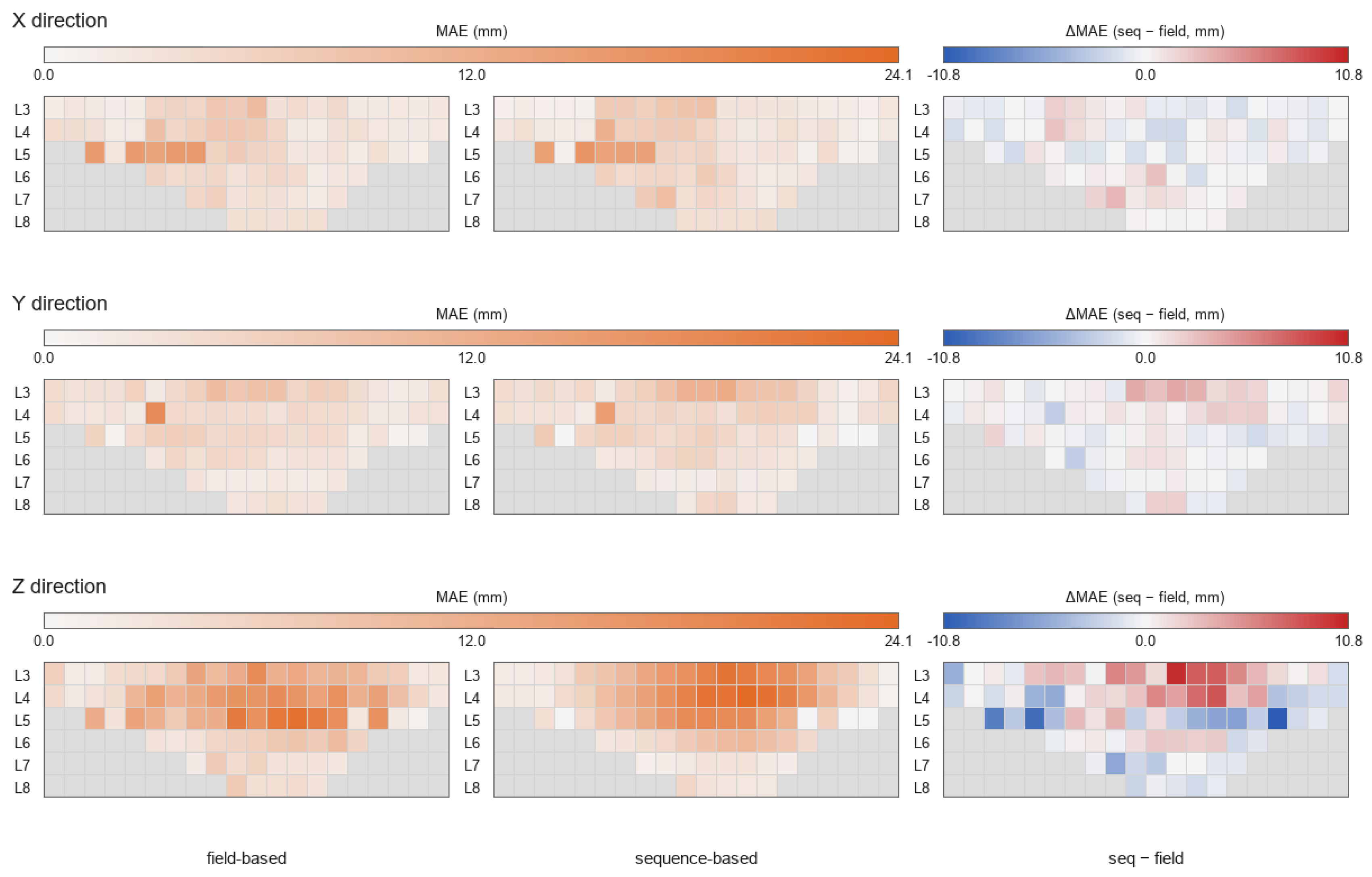
To further examine how route-level differences are distributed across the monitoring layout, the mean absolute error at each valid monitoring position is mapped back to the reconstructed displacement-field structure. The spatial MAE is averaged over the test samples and four representative forecasting horizons, namely t + 1, t + 7, t + 30, and t + 60. Figure 11 compares the spatial MAE distributions of the field-based and sequence-based routes for the X-, Y-, and Z-direction displacement components. The rightmost column shows the route-level difference, defined as the MAE of the sequence-based route minus that of the field-based route. Positive values therefore indicate locations where the sequence-based route produces larger errors, whereas negative values indicate locations where the field-based route produces larger errors.

The spatial patterns differ across the three displacement components. In the X direction, both routes show broadly comparable error levels over most valid positions, while the difference map reveals localized positive regions around the central part of the monitoring layout, especially near the L5 survey line. This indicates that the field-based route provides lower X-direction errors at several local positions, although the overall route-level difference remains limited.

In the Y direction, the two routes exhibit similar spatial MAE distributions, but the difference map still shows localized positive and negative differences. Several upper and central positions display positive values, indicating that the field-based route retains a local advantage in part of the monitoring layout. This pattern is consistent with the horizon-wise RMSE comparison in Figure 9, where the field-based route performs more favorably for the Y-direction displacement across the representative forecasting horizons.

The Z direction exhibits more pronounced spatial heterogeneity. The sequence-based route shows a broader high-error zone in the upper-central part of the monitoring layout, producing an extended positive region in the difference map. At the same time, several surrounding positions display negative differences, indicating that the sequence-based route performs better in other local areas. Although the sequence-based route achieves slightly lower route-level RMSE values for the Z-direction displacement in Table 7, the spatial maps show that this average advantage is not uniformly distributed across the monitoring layout. Instead, the two routes exhibit different local error patterns in spatially distinct monitoring regions.

The spatial error analysis complements the aggregate metrics and horizon-wise comparisons by preserving the physical location of each prediction deviation. Rather than relying only on route-level average errors, Figure 11 shows that the influence of the modeling route is spatially heterogeneous and depends on both the displacement component and the monitored region within the reconstructed field.

4.5. Engineering Applicability of the Forecasting Routes

In addition to forecasting accuracy, model selection for engineering deployment should consider computational cost, inference efficiency, and the ease of updating the model when the monitoring configuration changes.

Table 9. Engineering applicability comparison of the four forecasting models.

Model	Route Type	Total Parameters	Training-Step Time (ms)	Single-Sample Inference Latency (ms)	2D-Layout Dependence	Update Flexibility
SimVP	Field-based	2,356,836	455.781	4.686	Yes	Moderate; keep fixed 2D layout and neighborhood mapping.
SimVPv2	Field-based	41,550,720	94.078	5.2	Yes	Moderate; fixed matrix mapping is still required.
PatchTST	Sequence-based	22,458,464	72.578	4.582	No	Higher; mainly depends on flattened feature order.
TimesNet	Sequence-based	41,562,336	360.325	20.52	No	Higher; relies on flattened feature order and temporal-period modeling.

Note: Timing values are reported for relative comparison under the current computing environment rather than as cross-platform absolute benchmarks. SimVP keeps an explicit dependence on a fixed two-dimensional layout and neighborhood mapping. SimVPv2 also requires a fixed matrix mapping, although its internal feature-extraction mechanism differs from that of SimVP. PatchTST and TimesNet operate on flattened spatial variables and are therefore more flexible to reconfigure when the monitoring layout changes. However, feature-index remapping and model updating may still be required when monitoring points are added, removed, or rearranged.

compares the four models in terms of parameter scale, training-step time, single-sample inference latency, dependence on the reconstructed two-dimensional layout, and deployment-update flexibility. The reported timing values are intended for relative comparison under the current computing environment rather than as cross-platform absolute benchmarks.

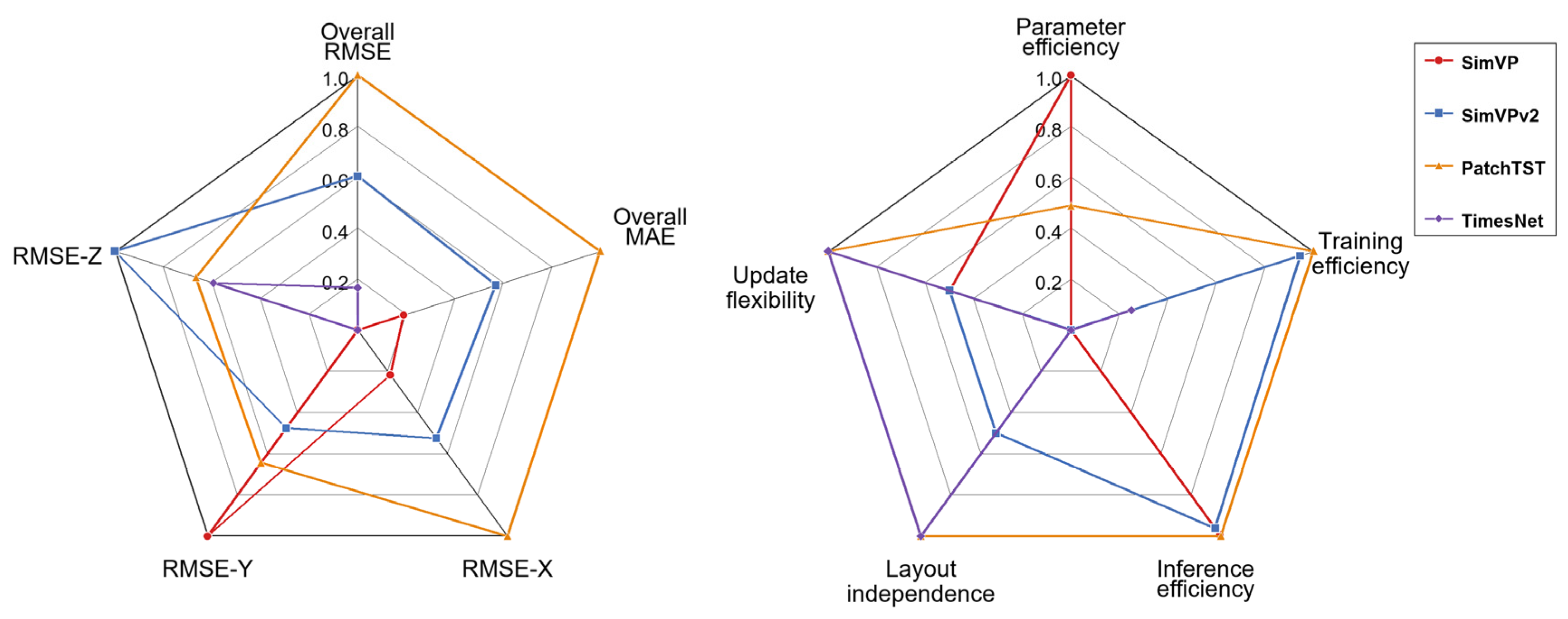
Figure 12 provides a normalized multi-criteria summary of the four forecasting models. No single model dominates across all predictive and engineering dimensions. PatchTST exhibits a relatively balanced profile in forecasting accuracy and computational efficiency, whereas SimVP retains an advantage in model compactness. SimVPv2 performs favorably in Z-direction forecasting, while TimesNet shows higher anticipated update flexibility but requires greater inference latency. These differences suggest that model selection should be aligned with the specific requirements of the operational monitoring scenario.

The results show that predictive performance and engineering efficiency do not follow a single ranking. SimVP has the smallest parameter scale among the four models, but it also has the slowest training-step time in the present environment. PatchTST achieves both the fastest training step and the lowest single-sample inference latency, while maintaining competitive forecasting performance in the overall comparisons. SimVPv2 has a substantially larger parameter scale but still maintains relatively low inference latency. By contrast, TimesNet shows the highest single-sample inference latency, making it less favorable for latency-sensitive deployment scenarios.

The two route types also differ in their dependence on the monitoring layout. SimVP explicitly uses the reconstructed two-dimensional displacement field and therefore requires a consistent spatial-neighborhood mapping when the monitoring network is updated. SimVPv2 also retains the field-oriented input object and requires a fixed matrix mapping. By contrast, PatchTST and TimesNet mainly rely on fixed variable ordering after sequence reformulation, meaning they are easier to reconfigure when monitoring points are added, removed, or rearranged. Nevertheless, feature-index remapping and model updating may still be required when the monitoring configuration changes.

These results indicate that the preferred model depends on the intended engineering scenario. Field-based models remain attractive when preserving spatial structure is an important consideration and the monitoring layout is relatively stable. Sequence-based models provide higher update flexibility when the monitoring configuration changes more frequently. The unified field-oriented forecasting framework developed in this study allows these models to be compared, selected, and updated within the same physical monitoring definition, providing a practical basis for model deployment in operational monitoring systems.

5. Discussion

5.1. Why Field-Oriented Representation Matters for Multi-Point Dam Monitoring

The present results show that the value of the proposed field-oriented forecasting framework does not depend on whether field-based models are uniformly superior to sequence-based models. Its main contribution is to provide a structured digital representation that preserves the ordered survey-line and monitoring-point organization of the monitoring system while supporting a common interface for different forecasting routes. Under this representation, field-based and sequence-based models can be trained, evaluated, and compared within the same physical monitoring definition, the same chronological split, and the same valid-position boundary. This makes route-level differences easier to interpret in engineering terms, because the comparison is less affected by inconsistencies in data organization or evaluation scope.

This point is particularly important for long-term multi-point dam monitoring, where observations are not an arbitrary collection of variables, but an ordered set of measurements associated with specific survey lines and structural zones. The reconstructed field should therefore be understood as a compact engineering data object rather than as a complete geometric or physical model of the dam body. Its practical value lies in preserving the monitoring layout in a form that remains compatible with different forecasting models, thereby supporting structured comparison, deployment-oriented analysis, and a consistent basis for subsequent model adaptation and updating.

5.2. Interpretation of Direction-Dependent and Horizon-Wise Forecasting Behavior

The comparison between the field-based and sequence-based routes indicates that forecasting behavior cannot be characterized adequately by a single overall metric. Although the aggregate differences between the two routes remain limited, their relative behavior varies across displacement components and forecasting horizons. This suggests that model selection for multi-point displacement forecasting should not be based only on route-level average RMSE or MAE, because such summaries can conceal directional and temporal differences that remain meaningful in engineering interpretation.

Under the present dam case and experimental configuration, the relative behavior of the two forecasting routes varies across displacement components and forecasting horizons. The Y-direction results indicate that the field-based route achieves lower errors under the current monitoring layout, whereas the sequence-based route remains competitive for the Z-direction response. The X-direction results exhibit a horizon-dependent transition rather than a stable advantage for either route. These observations should be interpreted as case-specific comparative evidence and do not establish that one forecasting route is generally more suitable for a particular displacement direction. At the same time, neither route exhibits evident progressive error amplification across the representative forecasting horizons. The main value of the proposed framework is therefore to reveal direction-, horizon-, and location-dependent differences under a unified physical monitoring definition, rather than to derive a universal direction-specific model-selection rule.

5.3. Methodological Role of the Valid-Position-Aware Protocol

The valid-position-aware protocol should be interpreted primarily as a methodological design that defines a physically meaningful loss and evaluation boundary. In the reconstructed 6 × 20 field, not all matrix positions correspond to actual monitoring points. Some entries are structural placeholders introduced only to maintain a unified spatial canvas for survey lines with unequal numbers of valid measurements. If these padded positions are treated as ordinary targets, the numerical objective no longer corresponds to the physical monitoring system that the model is intended to represent.

The ablation results further show why this protocol should not be presented as a universal performance-enhancement technique. Extending the loss calculation from valid monitoring positions to all matrix positions improves the valid-position validation RMSE for some models and worsens it for others. This mixed response indicates that the protocol does not act as a model-agnostic accuracy booster. Its main role is instead to ensure that optimization, checkpoint selection, and reported errors remain associated with real monitoring locations rather than with structural padding. In this sense, the protocol is important not because it guarantees better numerical performance, but because it preserves the physical meaning of the forecasting task and supports fair comparison within the same physical monitoring definition.

More broadly, this point is relevant beyond the present dam case. Engineering monitoring systems often involve irregular layouts, unequal section densities, and partially missing spatial coverage. When such systems are reorganized into structured digital objects, placeholders may be unavoidable for computational consistency. The present results suggest that these placeholders should be treated as devices of representation rather than as equivalent observations. Defining an explicit valid-position boundary is therefore essential for avoiding artificial dilution of reported errors and for keeping the learning objective aligned with the monitored physical system.

5.4. Implications for Engineering Deployment and Subsequent Model Adaptation

The engineering applicability results indicate that predictive accuracy, computational efficiency, layout dependence, and update flexibility do not follow a single ranking. Practical model selection should therefore depend on the operational context rather than on one preferred metric. When preservation of the monitoring layout is important and the configuration of monitoring points is relatively stable, field-based models remain attractive because they retain the structured field form throughout forecasting and maintain a clearer connection to the original monitoring arrangement. When the monitoring configuration is more likely to change, sequence-based models may offer greater flexibility because they depend less directly on fixed two-dimensional neighborhood relationships.

Even so, this flexibility should not be overstated. Sequence-based models may be easier to reconfigure, but feature-index remapping, model-specific input adaptation, and retraining may still be required when monitoring points are added, removed, or rearranged. Field-based models are likewise subject to constraints because the fixed matrix mapping must remain consistent with the defined monitoring layout. The engineering significance of the proposed framework therefore lies less in enabling unrestricted model substitutions than in providing a unified field-oriented object through which different models can be compared, selected, and subsequently adapted or retrained within the same physical monitoring definition.

5.5. Limitations and Future Work

Several limitations define the current scope of the study. First, the conclusions are drawn from a single high earth–rockfill dam with one long-term monitoring system. Although the dataset covers a substantial operational period, the generality of the findings should not be overstated. In addition, the reconstructed displacement field is a compact engineering representation rather than a full three-dimensional geometric or physical model. It preserves the ordered monitoring layout, but it does not explicitly encode geometric details, material zoning, hydraulic connectivity, or mechanical constraints. Further validation on additional dams and richer integration with structural context would therefore be necessary before extending the present conclusions to broader dam-monitoring scenarios. Accordingly, the direction-wise and route-level rankings observed in this study should be regarded as case-specific and require validation using additional dams, monitoring layouts, and operating conditions. Although causal forward filling avoids future-information leakage and preserves a continuous daily input sequence, it can generate piecewise-constant intervals and strengthen the apparent persistence of the displacement records, particularly for survey lines with relatively sparse direct observations. The daily grid should therefore be interpreted as a causal computational alignment of irregular engineering survey records rather than as a sequence of independently measured daily displacement observations. The observation-status channel enables models to distinguish directly observed and forward-filled inputs, but the reported forecasting performance should still be interpreted together with the survey-line-specific observation availability and forward-filling proportions.

Second, the present analysis focuses on four representative forecasting models and deterministic prediction accuracy. Although these choices are sufficient for clarifying the role of the field-oriented representation, route-level differences, and the valid-position-aware protocol, they do not exhaust the available modeling possibilities. Future work could incorporate additional model families, including graph-based forecasting approaches, physics-informed methods, and dynamics-informed predictors [12,18,19]. The framework could also be extended toward uncertainty-aware forecasting through probabilistic prediction, confidence intervals, and quantile-based prediction [20,21]. In addition, recent advances in signal decomposition and feature selection [22], dual-stage attention mechanisms [23], time-delay modeling [24], and SHAP-driven ensemble learning [25] may provide useful references for improving condition-aware forecasting and model interpretability. Further work could also investigate how predictive uncertainty varies under different operational scenarios, such as high-water-level periods, flood seasons, and low-temperature stages. Such extensions would be particularly valuable for engineering decision support, where predictive reliability, interpretability, and uncertainty quantification are as important as point accuracy.

Another limitation concerns the interpretation of sliding-window forecasting under slow long-term structural evolution. Because the models infer future displacement from recent historical records, a gradually developing trend may remain consistent with the recent input window and may therefore receive a relatively small prediction error. This issue may become more pronounced when the forecasting model is periodically retrained or updated using newly accumulated monitoring records, because a progressive change may gradually be incorporated into the learned representation of expected behavior. Consequently, close agreement between predicted and measured displacement should not be interpreted as evidence that progressive anomalies are absent. In engineering applications, long-term anomaly identification should therefore combine forecast-error monitoring with absolute-threshold checks, deformation-rate and acceleration analysis, change-point detection, environmental and operational interpretation, and expert assessment.

Finally, the proposed framework is intended for predictive monitoring rather than direct safety diagnosis. Forecasting results should not be interpreted as standalone evidence of structural risk, because safe engineering judgment also requires threshold rules, deformation-rate analysis, environmental interpretation, and expert review. The present framework should therefore be viewed as a component of a broader digital monitoring workflow. Its most appropriate future extension is not simply toward larger model comparisons, but toward more integrated monitoring and decision-support systems in which forecasting is combined with physically informed interpretation and operational risk assessment.

6. Conclusions

This study developed a field-oriented forecasting framework for multi-point dam displacement prediction by reconstructing long-term monitoring records into a unified displacement-field object and comparing field-based and sequence-based modeling routes under a consistent chronological split, prediction task, normalization procedure, and valid-position evaluation boundary. Using long-term monitoring data from the Tianshengqiao First Dam, four representative models, namely SimVP, SimVPv2, PatchTST, and TimesNet, were evaluated from the perspectives of overall accuracy, horizon-wise behavior, spatial error distribution, validation-based ablation of the valid-position-aware loss boundary, and engineering applicability.

The results show that the proposed representation provides a physically consistent basis for organizing irregular multi-point monitoring records. Its value does not lie in guaranteeing universal numerical superiority for a particular forecasting route. Instead, it preserves the ordered monitoring layout, supports fair comparison among different model families, and enables direction-wise, spatial, and deployment-oriented analysis under a unified digital representation. The comparative results further indicate that forecasting performance is direction-dependent, horizon-dependent, and spatially heterogeneous, and that no single model or route dominates uniformly across all displacement components and forecasting horizons.

The valid-position-aware protocol should be understood primarily as a methodological design for defining a physically meaningful loss and evaluation boundary rather than as a universal performance-enhancement technique. Its main role is to ensure that optimization, checkpoint selection, and reported errors remain associated with actual monitoring positions rather than with structural placeholders introduced to maintain a fixed matrix form. The engineering applicability analysis further shows that predictive accuracy, computational efficiency, layout dependence, and model-adaptation flexibility do not follow a single ranking. Field-based models remain attractive when preserving the ordered monitoring layout is important and the monitoring configuration is relatively stable, whereas sequence-based models may offer greater flexibility when the monitoring configuration is more likely to change, although model-specific adaptation and retraining may still be required.

Several limitations remain. The present conclusions are drawn from a single high earth–rockfill dam, and the reconstructed displacement field is a compact engineering representation rather than a complete geometric or physical model. Future work should evaluate the framework on additional dam cases, incorporate richer structural and geometric information, and extend the analysis toward uncertainty-aware forecasting and integrated digital monitoring applications. Overall, the proposed framework provides a practical basis for comparing, selecting, and subsequently adapting forecasting models for multi-point dam displacement monitoring under a unified engineering data structure and a consistent physical monitoring definition.