
Article

A Practical Approach for Determining Depth-Dependent Mechanical Properties of Soft Materials in AFM Indentation via Polynomial Fitting and a New Model for Cellular Mechanics


by
Stylianos Vasileios Kontomaris
1,*,
Anna Malamou
2,*,
Ioannis Psychogios
3 and
Andreas Stylianou
1,*
1
Cancer Mechanobiology and Applied Biophysics Group, School of Sciences, European University Cyprus, Nicosia 2404, Cyprus
2
BioNanoTec Ltd., Nicosia 2043, Cyprus
3
Department of Engineering and Construction, Metropolitan College, 15125 Athens, Greece
*
Authors to whom correspondence should be addressed.
Submission received: 31 December 2025 / Revised: 2 February 2026 / Accepted: 6 February 2026 / Published: 9 February 2026
(This article belongs to the Section Materials Engineering)

Abstract

In most AFM nanoindentation experiments on soft biological samples, classical contact mechanics models, such as Hertz or Sneddon’s equations, are commonly employed to determine the Young’s modulus. However, biological materials are inherently heterogeneous, and their mechanical properties often depend on the indentation depth. In this work, we present a novel and simple approach to quantify how the apparent modulus varies with increasing indentation depth. The method is based on the general indentation equation for axisymmetric indenters combined with a straightforward polynomial fitting of the force–indentation data. The proposed approach offers significant advantages, as it greatly simplifies the fitting process without requiring any advanced algorithms, while maintaining high accuracy. In addition, it is shown that the depth-dependent mechanical properties of cells can be described by a simple law, E ( h ) = C d / h + E l , where E l is the limiting value of the apparent modulus at large indentations, and C d / h represents the depth-dependent contribution dominant at the initial stages of the indentation process. Here, C d is a positive stiffness coefficient, and h is the indentation depth. This is a very important result, indicating that by using the pair of coefficients C d and E l , we can fully describe the mechanical properties of cells, capturing their depth-dependent mechanical behavior. Experiments on fibroblasts and H4 human glioma cells confirm the accuracy of this equation. The proposed methods provide an accessible and reliable framework for nanoscale mechanical characterization, offering insights into the depth-dependent elasticity of heterogeneous soft materials and revealing mechanical patterns in biological samples.

1. Introduction

Atomic force microscopy (AFM) nanoindentation has become a key technique in biomedical research, allowing quantitative measurement of the mechanical properties of biological materials with nanometer spatial resolution and pico- to nano-Newton force sensitivity [1,2,3,4]. This capability has enabled the study of cell and tissue biomechanics, with mechanical properties emerging as potential biomarkers of physiological and pathological states. As a result, AFM is increasingly recognized as a promising tool for early disease detection, particularly in cancer, and is gradually moving from research toward clinical application [2,5,6,7,8,9]. It is important to note that several experimental techniques, such as atomic force microscopy (AFM), optical tweezers (OT) [10,11], and multifrequency magnetic resonance elastography (MMRE) [12], are widely used for the investigation of biomechanical properties across different length scales. Among these techniques, AFM offers a major advantage in terms of force sensitivity and dynamic range, as it can apply and measure forces from a few piconewtons up to tens, or even hundreds, of nanonewtons [13]. This range is significantly broader than that accessible by OT, which are typically limited to forces in the tens to hundreds of piconewtons [14]. As a result, AFM is particularly well suited for probing stiff biological structures and large deformations. Owing to this versatility, AFM can be applied to a wide variety of biological samples, ranging from soft living cells [15] to hard structural components such as collagen fibrils measured in air [13]. In addition, AFM provides nanometer-scale spatial resolution, enabling mechanical characterization at the level of single molecules, macromolecular assemblies, and individual cells. In contrast, MMRE is inherently limited to millimeter-to-submillimeter spatial resolution [12] and is therefore primarily restricted to tissue- and organ-level mechanical assessment.
Analysis of AFM nanoindentation data has largely relied on Hertzian contact mechanics to extract elastic moduli from force–indentation curves, producing a substantial and influential body of literature over the past two decades [16,17,18,19,20,21,22]. However, reliably determining the Young’s modulus of soft biological specimens remains challenging due to nanoscale heterogeneity and experimental uncertainties in cantilever deflection sensitivity and spring constant calibration [23,24]. In particular, the choice and validity of the contact mechanics model are critical, as biological systems rarely conform to the idealized assumptions of classical formulations [24].
Specifically, Hertzian contact mechanics was originally formulated to describe materials that are homogeneous, isotropic, and mechanically uniform [24]. In contrast, biological samples are naturally heterogeneous at the nanoscale, with complex structural and compositional variations that strongly affect their mechanical behavior. As a result, the apparent mechanical response can change with indentation depth, causing the measured modulus to either decrease (“softening”) or increase (“stiffening”) as the probe moves deeper into the material [23]. For this reason, the Young’s modulus obtained through Hertzian-based analyses is commonly denoted as an “apparent” Young’s modulus, reflecting its dependence on the indentation depth rather than a true, intrinsic material constant, and it is therefore highly sensitive to the chosen loading conditions and indentation range [25,26]. Within this context, many research groups have proposed methods for the accurate mechanical characterization of biological materials at the nanoscale [27]. Amo et al. demonstrated that bimodal AFM can be employed for the precise determination of surface elastic moduli in liquid environments, achieving an exceptional spatial resolution on the order of 3 Å [28]. Doss et al. introduced an analytical model for the interpretation of force–indentation data obtained from two-layer elastic systems [29]. Their analysis revealed that the mechanical influence of the underlying layer can be systematically predicted and effectively described through an analogy with Hookean springs connected in series. The proposed model remains valid for Young’s modulus mismatches spanning up to two orders of magnitude, provided that the contact radius remains smaller than the thickness of the upper layer [29]. More recently, Chen et al. proposed a comprehensive and robust theoretical framework, termed trimechanic theory, designed to capture the elastic responses of soft materials and biomaterials under a broad range of mechanical conditions [30]. Within this framework, variations in elastic behavior are interpreted as direct manifestations of changes in the material’s mechanical context. Trimechanic theory enables the systematic quantification of elastic response differences through combinations of three distinct nanomechanical actions, governed respectively by constant, linear, and nonlinear force contributions [30]. Notably, this theory emerges naturally from an extension of Sneddon’s pyramidal indenter model, specifically tailored to investigate elastic heterogeneity at the nanoscale [30].
In addition, other studies have aimed to extend the applicability of Hertzian-based formulations to heterogeneous materials by considering a broad range of indenter geometries, including cylindrical, parabolic, conical, spherical, and, more generally, arbitrarily shaped axisymmetric indenters [31,32]. These models are typically derived from energy-equivalent experiments or from the weighted mean value theorem for integrals. Under such conditions, three-dimensional nanomechanical characterization of soft, heterogeneous samples becomes feasible [31]. In addition, Ding et al. reported that AFM-based measurements performed on cells are strongly influenced by surface tension effects [26]. By combining dimensional analysis with finite element simulations, they demonstrated that, for cells indented with either a conical or a parabolic probe, a two-term power-law expression is appropriate for describing the depth-dependent mechanical properties of cells [26].
This paper addresses a classical problem in mechanobiology related to the development of improved techniques for disease diagnosis, with particular emphasis on cancer. The determination of Young’s modulus at different nanoregions of cells and tissues provides a mechanically driven pathway for early cancer detection and treatment monitoring, as cancer cells are typically softer than healthy ones [1]. Moreover, during cancer progression, a two-peak distribution of Young’s modulus may emerge due to the concurrent softening of cancer cells and stiffening of the extracellular matrix [2].
The strong mechanical heterogeneity of cells and biological tissues, however, can lead to significant inaccuracies when conventional Hertzian models are applied to indentation data. To overcome this limitation, we propose a simple and accurate approach for the nanoscale mechanical characterization of heterogeneous biological materials. The method is based on the generic force–indentation relationship for axisymmetric indenters combined with a straightforward polynomial fitting procedure. It yields a depth-dependent description of cellular mechanics using only two parameters: a stiffness coefficient that captures the pronounced heterogeneity at small indentation depths and a limiting elastic modulus representative of larger indentations. This framework enables reliable nanomechanical characterization and holds strong potential for applications in early cancer diagnostics, disease progression monitoring, and evaluation of therapeutic efficacy, while also being extendable to tissue engineering, regenerative medicine, and pharmaceutical research.
This paper is organized as follows: In Section 2, the new model is presented, along with the protocol for obtaining force–indentation curves from fibroblasts (open-access data) and H4 human glioma cells. In Section 3 (Results), the proposed approach is applied to cell force–indentation data, and the equation for capturing the full mechanical behavior of cells, from shallow to deep indentations, is tested. The results obtained using the method introduced in this paper are also compared with those derived from classic fitting procedures based on Hertzian equations. In Section 4 (Discussion), the advantages of the proposed approach over other methods, as well as its limitations, are discussed.

2. Materials and Methods

2.1. Deriving a New Model

Pharr et al. [33] derived a general equation linking the contact stiffness, that is, the derivative of the applied force with respect to indentation depth, to the material properties and the contact radius, as follows:
d F d h = 2 E * R c
where E * is the reduced modulus of the material, defined as E * = E 1 v 2 , with E and v being the Young’s modulus and Poisson’s ratio respectively. It should be noted at this point that the reduced modulus E * is generally defined by the following Equation: 1 E * = 1 v 2 E + 1 v i 2 E i [33]. Here, E , E i , v , v i denote the Young’s moduli and Poisson’s ratios of the sample and the indenter, respectively. However, since AFM tips are orders of magnitude stiffer than biological samples under physiological conditions (a typical silicon nitride AFM tip has a Young’s modulus in the range of 280–290 GPa [34]), it can be assumed that E i E , leading to E * = E 1 v 2 .
In addition, F denotes the applied force, h is the indentation depth and R c represents the contact radius between the indenter and the sample. It is important to note that Equation (1) was derived for materials that can be considered elastic half-spaces. An elastic half-space is a homogeneous, isotropic, and linearly elastic solid that extends infinitely in all directions beneath a plane surface. It is assumed to be semi-infinite in both depth and lateral dimensions so that boundary effects at the edges can be neglected. When a cylindrical (flat punch) indenter is used on an elastic half-space, the contact radius remains constant throughout the indentation and is equal to the actual radius of the indenter. In this case, the force–indentation relationship is linear. For other indenter geometries, however, the contact radius varies with indentation depth. In the case of heterogeneous materials, the slope of the force–indentation curve depends on the varying contact radius and the material’s depth-dependent mechanical properties [35]:
d F d h = 2 E * h R c ( h )
Therefore, by calculating the slope of the force–indentation curve at a given point and subsequently solving Equation (2) for E * ( h ) , the local mechanical properties of the material at the corresponding indentation depth can be determined. A polynomial fit can effectively capture the nonlinear relationship between force and indentation depth, which commonly arises in real materials due to complex mechanical behavior. In particular, soft biological samples often display significant nanoscale heterogeneity, rendering classical fitting approaches based on Hertzian equations inadequate. For indenters with non-flat punch geometries, the nonlinear behavior of the force–indentation data within the traditional Hertzian framework is attributed to the variation in the contact radius with indentation depth. In contrast, a polynomial fit can account for nonlinearities arising both from the material’s heterogeneity and from the depth-dependent variation of the contact radius. Therefore, we employ the following equation for data fitting:
F = n = 1 m c n h n = c 1 h + c 2 h 2 + + c m h m
where c 1 , c 2 , , c m are fitting constants. It should be noted that for h = 0 , F = 0 ; this is the reason for not including a c 0 term in the fitting. The derivative of Equation (3) can be readily calculated as follows:
d F d h = d d h n = 1 m c n h n = n = 1 m n c n h n 1 = c 1 + 2 c 2 h + + m c m h m 1
Equation (4) can be combined with Equation (2) to determine the depth-dependent mechanical properties of the sample of interest:
E * h = 1 2 R c ( h ) n = 1 m n c n h n 1
In particular, for a biological sample under physiological conditions, where the water content is high, ν = 0.5 ; therefore, we obtain
E ( h ) = 3 8 R c ( h ) n = 1 m n c n h n 1
For the case of classical pyramidal indenters, which are typically approximated as perfect cones when the indentation depth is significantly larger than the tip radius [36],
R c , c o n e h = 2 π tan θ h
where θ is the cone’s semi-included angle. The contact depth and contact radius when using a conical indenter is shown in Figure 1a. By combining Equations (6) and (7), we obtain
E c o n e ( h ) = 3 π 16 tan θ h n = 1 m n c n h n 1  
In addition, for spherical indenters, the accurate equation relating the contact radius to the indentation depth for deep indentations was originally derived by Sneddon [37,38]:
h = R c 2 ln R + R c R R c
Equation (9) cannot be solved with respect to R c . By considering the variable R c / R and using a Taylor series expansion around R c / R = 0 , we conclude the following:
R c , s p h e r e = R 3 2 1 + 1 + 4 3 h R
The contact depth and contact radius when using a spherical indenter is shown in Figure 1b. The full derivation of Equation (10) is presented in Appendix A. Finally, by combining Equation (6) with Equation (10), the following conclusion can be drawn:
E s p h e r e ( h ) = 3 8 R 3 2 1 + 1 + 4 3 h R n = 1 m n c n h n 1
For small indentation depths compared to the tip’s radius ( h < < R ), the parabolic approximation can be used [36]:
R c , p a r a b o l o i d = R h
In this case, Equation (6) is written as follows:
E P a r a b o l o i d ( h ) = 3 8 R h n = 1 m n c n h n 1
In Figure 1c we compare the R c / R ratios with respect to h / R when using Equation (10) (Spherical indenter) and when using the parabolic approximation (Equation (12)). For h R , these Equations lead to identical results as expected.

2.2. Proposing a New Model for Cellular Mechanics

Different studies in the literature have shown that the apparent Young’s modulus of biological cells is strongly depth-dependent, following a characteristic pattern [25,26,27]. Specifically, the apparent modulus decreases with increasing indentation depth, approaching a limiting value at large indentations [25,26,27]. Several mathematical models have been proposed to describe and capture this depth-dependent mechanical behavior [25,26,27], highlighting the need for accurate frameworks that account for cellular heterogeneity and the variation in stiffness across different indentation scales. In this paper, we propose the simplest law to capture this behavior, as described below:
E h = C d h + E l
where E l is the limiting value of the apparent modulus for large indentations, and C d / h is a term describing the depth-dependent properties at the initial stages of the indentation process. Here, C d is a positive stiffness coefficient describing the initial behavior of the cell at small depths, and h is the indentation depth. The selection of this specific equation is motivated by both physical and practical considerations. The term C d / h captures the pronounced increase in stiffness observed at shallow indentation depths, which reflects the near-surface mechanical response of cells, including contributions from the cortex and membrane structures. As the indentation depth increases, these surface effects diminish, and the modulus gradually approaches the limiting value E l , representing the bulk mechanical behavior of the cell interior. The simplicity of the equation ensures ease of fitting to experimental data while remaining physically interpretable, requiring only two meaningful parameters to fully describe the depth-dependent mechanical response. In other words, instead of performing classic Hertzian fitting procedures to determine the sample’s apparent modulus at a single point, which strongly depends on the indentation depth, the methods presented in this paper, together with Equation (14), allow the determination of two material constants, namely C d and E l , which accurately describe the mechanical behavior of the cell across all scales.
The objective is to propose the simplest possible model involving only two fitting parameters. However, it should be noted that the C d / h term diverges as h 0 ; this may be regarded as a potential drawback of the model. Nevertheless, there is no point in testing the model behavior at h = 0 , since no indentation occurs at this point. Consequently, examining the validity of the proposed model at this point is not meaningful. The analysis can always start from the first non-zero h , F data point, for which the model remains valid (for both perfect conical and spherical indenters). From this perspective, introducing an additional fitting parameter would unnecessarily increase the complexity of the model and the fitting procedure.
It is also important to note that Equation (14) represents a specific subcase, suitable for fitting data derived from Equation (6) in the particular case of cells. It is unsuitable for stiffening materials and is instead a convenient model specifically tailored for cellular systems. However, by using the general approach presented in this paper (Equations (1)–(6)), it is straightforward to derive appropriate expressions for other types of samples, including those exhibiting softening or hardening behavior.

2.3. Open Access Data from Fibroblasts and H4 Human Glioma Cells

To validate the proposed method, we utilized open-access nanoindentation data from fibroblasts [39]. The experiments were performed using a conical indenter with a half-angle of 25° and a cantilever with a spring constant of 0.01 N m−1 [39]. The corresponding force–indentation datasets supporting the results of this study are publicly available in the AtomicJ repository (https://sourceforge.net/projects/jrobust/files/TestFiles/), accessed on 1 December 2025. Additionally, previously published spherical nanoindentation data from H4 human glioma cells (ATCC) were used [40]. In these experiments, a ball-shaped tip with a radius of 2.5 μm and a cantilever spring constant of 0.08 N/m (measured using the thermal noise method) was employed. In both fibroblasts and H4 human glioma cells, only force curves obtained from the central region of the cells were taken into account to avoid substrate effects. The accuracy of each fitting procedure was evaluated using the R-squared coefficient ( R s . c . 2 ) with values close to 1 indicating a high-quality fit.

3. Results

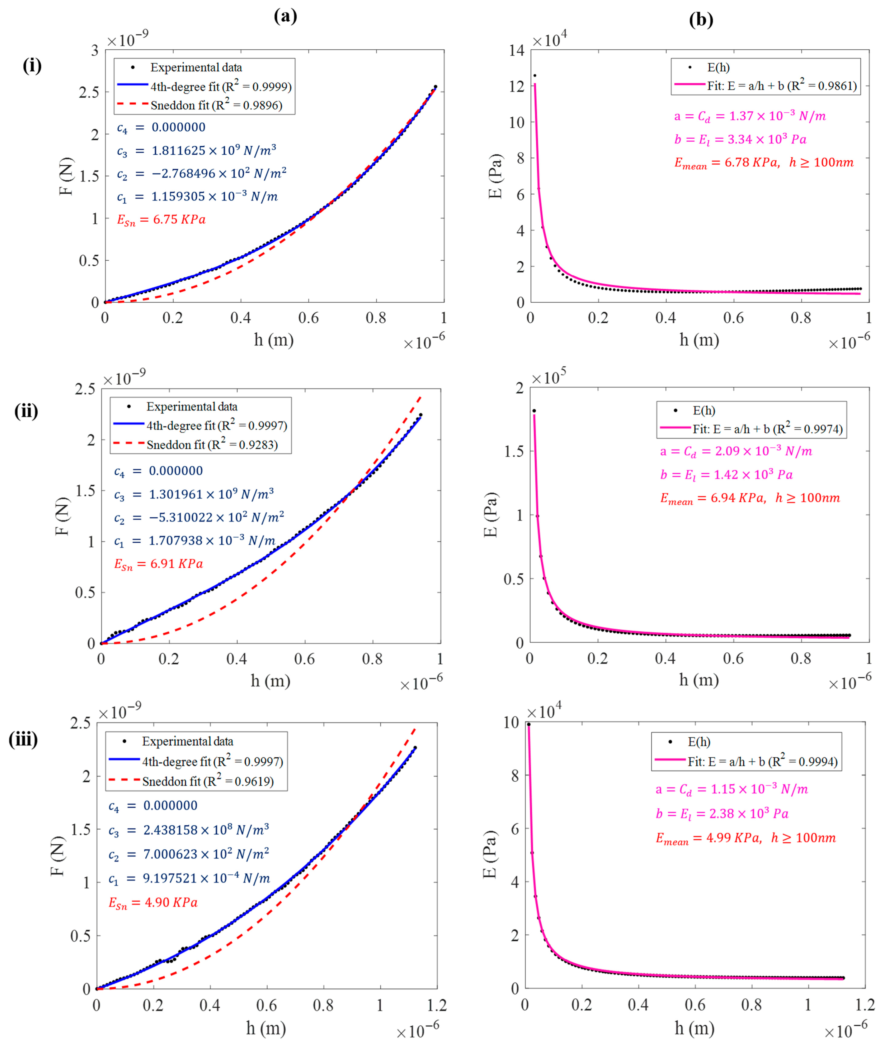
In Figure 2, three characteristic cases of force–indentation curves from fibroblasts are presented (Figure 2(ai–aiii)). To capture extreme cases of mechanical heterogeneity, a fourth-degree polynomial was used, as shown below:
F = n = 1 4 c n h n = c 1 h + c 2 h 2 + c 3 h 3 + c 4 h 4
Although the fitting process often yielded c 4 = 0 , indicating that a third-degree polynomial could adequately describe the data, a fourth-degree polynomial was retained to provide additional flexibility. This choice enables the capture of subtle variations and extreme behaviors in the force–indentation curves while preserving the overall measurement trends. In this sense, the fourth-degree polynomial represents a balance between flexibility and robustness when modeling mechanically heterogeneous biological samples. Higher-degree polynomials were avoided as they increase sensitivity to noise and the risk of overfitting without offering meaningful improvements in fit quality or physical interpretability.
We should emphasize here that a fourth-degree polynomial does not represent a more accurate physical model or a generalization of Sneddon’s equation. It is simply a convenient tool to closely follow the data and to easily compute the contact stiffness from Equation (4) for use in Equation (2).
The fitting coefficients are shown within the figures in all cases. In addition to the fourth-degree polynomial, the classic Sneddon’s equation was also fitted for comparison [26]:
F = C S n h 2
where C S n = 2 π E * tan θ . Each graph displays the R-squared coefficients for both the polynomial and Sneddon’s fits. Subsequently, the mechanical properties for each case were determined using both the proposed approach and the classic Sneddon’s fit. Specifically, the elastic modulus was calculated at each indentation depth using Equation (8), and the resulting E = f ( h ) curves are presented in Figure 2(bi–biii). The data were then fitted to Equation (14), yielding a simple pair of values, C d and E l , that can accurately describe the cellular behavior at any indentation depth.
It is important to note that using Equation (14), we can easily relate the results to Sneddon’s fitting. First, the tip radius of the conical indenter used in the experiments was 20 nm. To apply a perfect cone approximation, as assumed in the derivation of Equation (8), the indentation depth should satisfy h R tip . Therefore, only data with h 100 nm were considered, and the mean value of the function given by Equation (14) was calculated:
E m e a n ( c o n e ) = 1 h m a x h m i n h m i n h m a x C d u + E l d u E m e a n ( c o n e ) = C d h m a x h m i n l n h m a x h m i n + E l
Here, h min = 100 nm, h max is the maximum indentation depth, “ l n ” denotes the natural logarithm, and u is a dummy integration variable. The calculated E mean is shown in Figure 2(bi–biii) and is nearly identical to the results obtained from Sneddon’s fit in all cases. It should be clarified that the force–indentation fitting and the derivation of the depth-dependent modulus E ( h ) were performed using the full indentation range, without excluding shallow depths. The indentation cutoff was applied only to the calculation of the mean elastic modulus in Equation (17), and not during the fitting or differentiation steps. Because the AFM tip has a rounded apex, its geometry is not perfectly conical; therefore, at very small indentation depths, the extracted Young’s modulus values are not reliable. A conical approximation becomes valid when the indentation depth is sufficiently large compared to the tip radius. For this reason, shallow depths were excluded solely from the averaging procedure. A cutoff of h min = 100   n m (approximately 5 R t i p , with R t i p 20   n m ) was selected as a conservative threshold. The resulting mean modulus was found to be nearly identical to that obtained using a classical Sneddon fit in this case. If a threshold that is too small is used, numerous spurious (“false”) values contribute to the average. Conversely, using a very large indentation depth to ensure a perfect conical approximation would lead to a loss of information associated with the initial heterogeneous regime of the cell. Using a threshold equal to 5 R t i p resulted in equivalent results to those obtained with the classical Sneddon fitting approach.
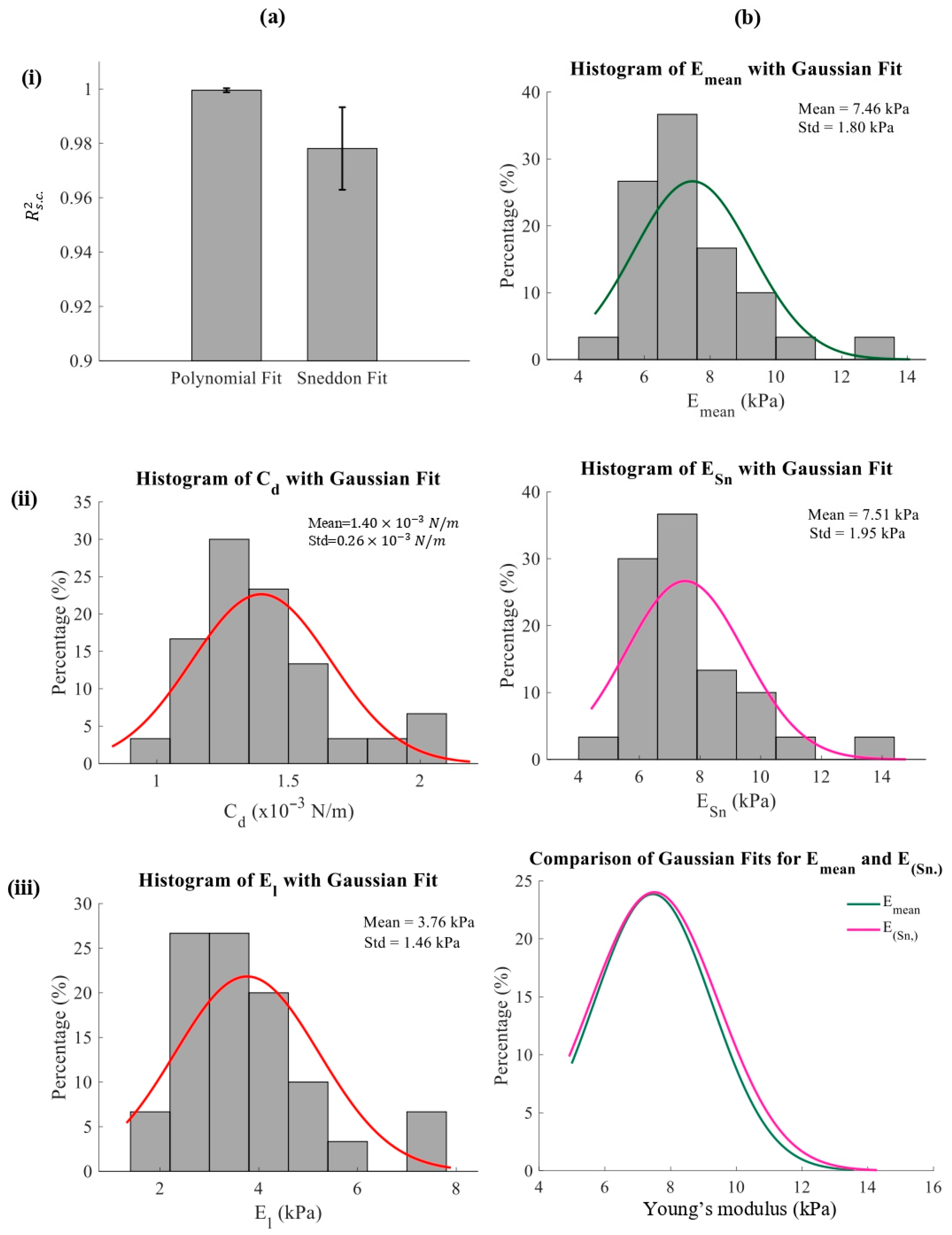
In Table 1, we also present 30 measurements on fibroblasts. Specifically, the first two columns show the R-squared coefficients for the fourth-degree polynomial fit and the Sneddon’s fit, respectively. The third and fourth columns report the coefficients C d and E l , respectively, while the fifth column shows the R-squared coefficient obtained when fitting the E = f ( h ) data to Equation (14). Finally, the sixth and seventh columns present the E mean values calculated using Equation (17) and the Young’s modulus obtained from Sneddon’s fit, respectively. The results presented in Table 1 are also highlighted in Figure 3. Bar charts of the R-squared coefficients for the 4th-degree polynomial fit and the Sneddon fit, including error bars for each case, are presented in Figure 3(ai). The mean ± standard deviation values were 0.99955 ± 0.00073 for the polynomial fit and 0.97812 ± 0.01520 for the Sneddon fit, indicating that the polynomial fitting approach provides higher consistency and accuracy.
In Figure 3(aii,aiii), histograms of the C d and E l values are presented along with Gaussian fits. The mean ± standard deviation values are C d = ( 1.40 ± 0.26 ) × 10 3 N/m and E l = 3.76 ± 1.46 kPa. In addition, Figure 3(bi,bii) show the E m e a n and E S n values, corresponding to the mean modulus obtained from the proposed model using Equation (17) and the modulus calculated from the Sneddon fit, respectively. The mean ± standard deviation values are E m e a n = 7.46 ± 1.80 kPa and E S n = 7.51 ± 1.95 kPa. Finally, Figure 3(biii) compares the Gaussian fits for E mean and E Sn , showing that the mean value of Equation (14) closely matches the results obtained using the classic Sneddon fit.
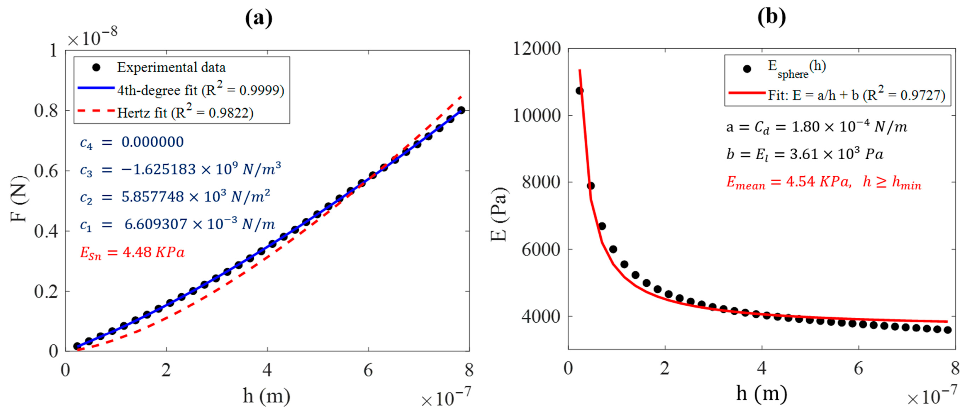
We also present additional measurements performed using a spherical indenter on a H4 human glioma cell, following the protocol described in Section 2.3. A representative force–indentation curve obtained with the spherical indenter is shown in Figure 4. A fourth-degree polynomial fit, as well as an extended Hertzian fit for large indentations, were also applied. In particular, for h 1.5 R , the accurate force–indentation equation for spherical indenters is presented below [41,42,43]:
F = C H e r t z h 3 2 1 h 10 R  
where C Hertz = 4 3 E 1 v 2 R 1 / 2 .
The fitting coefficients for the polynomial fit and the results from the Hertzian fitting are shown in Figure 4a. In Figure 4b, the E = f ( h ) data are shown along with a fit to Equation (14) proposed in this paper.
The fitting parameters are also presented within the graph. It is important to note that a mean apparent modulus was obtained in this case as well, for comparison with the result derived from fitting Equation (18). However, since a spherical indenter was used, it is unnecessary to restrict the minimum indentation depth to 100 nm, as was done for the conical indenter in fibroblasts. In this case, the minimum indentation depth corresponds to the first data point in the h , F pair, that is, the initial point of the force–indentation curve. The mean apparent modulus was found to be nearly identical to that obtained from the Hertzian fit (using the extended Hertzian Equation (18)).
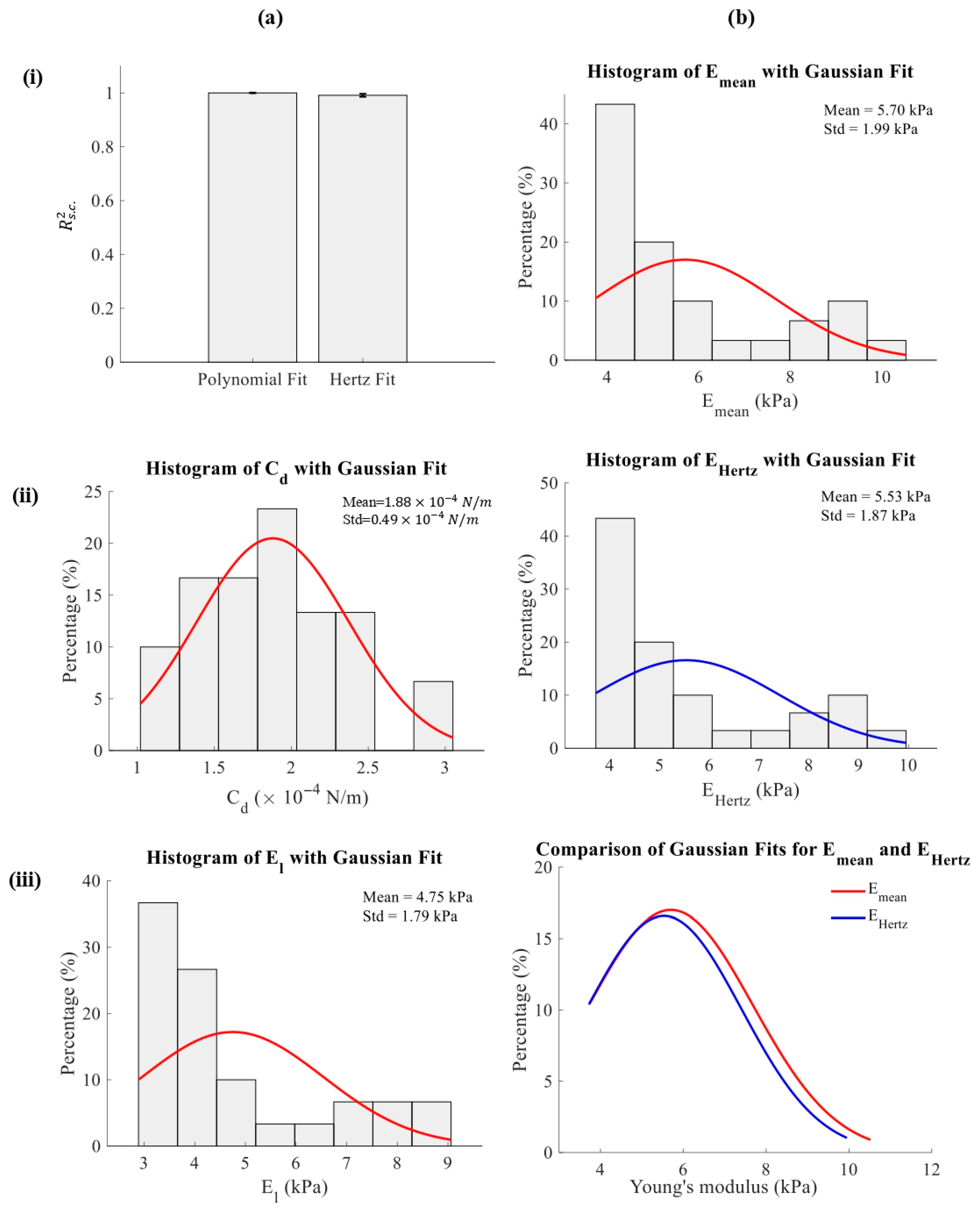
Table 2 also presents 30 measurements on a H4 human glioma cell. The first two columns report the R-squared coefficients for the fourth-degree polynomial and Hertzian fits, respectively (i.e., Equation (18)). Columns three and four show the coefficients C d and E l , while the fifth column provides the R s . c . 2 value obtained from fitting the E = f ( h ) data to Equation (14). The sixth and seventh columns present the mean apparent modulus ( E mean ) calculated using Equation (17) and the Young’s modulus from the Hertzian fit, calculated using Equation (18), respectively. The results in Table 2 are also highlighted in Figure 5.
Bar charts of the R 2 coefficients for the fourth-degree polynomial and Hertzian fits, including error bars for each case, are shown in Figure 5(ai). The mean ± standard deviation values were 0.99989 ± 0.00008 for the polynomial fit and 0.99119 ± 0.0055 for the Hertzian fit. In Figure 5(aii,aiii), histograms of the C d and E l values are presented along with Gaussian fits. The mean ± standard deviation values are C d = ( 1.88 ± 0.49 ) × 10 4 N/m and E l = 4.75 ± 1.79 kPa. In addition, Figure 5(bi,bii) show the E m e a n and E H e r t z values, corresponding to the mean modulus obtained from the proposed model using Equation (17) and the modulus calculated using Equation (18), respectively. The mean ± standard deviation values are E m e a n = 5.70 ± 1.99 kPa and E H e r t z = 5.53 ± 1.87 kPa. Finally, Figure 5(biii) presents a comparison of the Gaussian fits for E mean and E Hertz , demonstrating that the proposed generic method can also closely reproduce the results obtained with the Hertzian fit through the mean value of Equation (14), i.e., Equation (17).

4. Discussion

In this paper, a new approach for the mechanical characterization of soft materials is proposed, based on a simple polynomial fitting and the generic nanoindentation equation that relates the contact stiffness, S = d F / d h , to the material properties and the contact radius between the indenter and the sample (Equation (1)). In this way, the depth-dependent mechanical properties of soft biological samples can be revealed. Particular attention should be given to the case of spherical indenters, for which the contact radius between the indenter and the sample is described by Equation (10). Equation (12) represents the parabolic approximation and is valid only for very small indentation depths compared to the tip radius. A typical limit in the literature is h < R / 10 [44,45].
Besides proposing a new approach for the mechanical characterization of soft samples, a simple equation is also introduced to describe the depth-dependent mechanical properties of biological cells (Equation (14)). This equation is motivated by observations from numerous AFM nanoindentation studies reported in the literature, which consistently show that the apparent Young’s modulus decreases with increasing indentation depth and eventually approaches a limiting value [25,26,27]. Several models have been proposed to capture this behavior. However, the approach proposed in this paper has the major advantage of fully characterizing the mechanical response of cells using only two parameters: C d , a positive constant associated with the strongly heterogeneous structure of the cell at shallow indentation depths, and the limiting modulus E l .
The proposed equation (i.e., Equation (14)) was tested using open-access indentation data from fibroblasts, as well as indentation experiments on H4 human glioma cells, following the protocols described in Section 2.3. In all cases, Equation (14) accurately captures the mechanical behavior of the cells. Moreover, the proposed method yields results that are consistent with those obtained using classical fitting procedures, namely Sneddon’s model for conical indenters and the modified Hertzian equation for spherical indenters, by considering the mean value of Equation (14), as expressed in Equation (17). Special attention should be given to pyramidal and conical indenters with a rounded tip apex. In the case examined in this paper, a minimum indentation depth of 100 nm was used as the lower limit of the integral in Equation (17), since the tip apex radius of the indenter was 20 nm and the conical approximation is valid only when the indentation depth is significantly larger than the tip radius. Accordingly, in Equation (17), the integration limits were set to h m i n = 100   nm and h m a x , where h m a x corresponds to the maximum indentation depth for each individual measurement. In contrast, for spherical indenters, no such limitation applies. In this case, the minimum indentation depth used in Equation (17) was taken as the smallest measured value, that is, the minimum h in the set of recorded (h, F) data pairs.
The new model for cells (i.e., Equation (14)) provides significant advantages over classic Hertz–Sneddon fits. This is because it describes the mechanical heterogeneity of a cell at a single location using only a pair of constants, C d and E l . In contrast, results obtained using classical fitting approaches are strongly dependent on indentation depth. Consequently, two mechanical property maps, one for C d and one for E l , contain all the information required to fully characterize the depth-dependent mechanical behavior of a cell over extended regions. Equation (14) is also advantageous compared to more complicated approaches, as it requires the minimum number of constants, all of which have clear physical significance. Specifically, the constant C d characterizes the superficial regions of the cell, while E l represents its bulk mechanical properties.
Despite the accuracy of the proposed method, it is not free of limitations. An important limitation is that it cannot be applied to samples of finite thickness. This is because the determination of the Young’s modulus for homogeneous samples with finite thickness relies on the classical Hertzian–Sneddon equations supplemented by appropriate series correction factors [46,47,48]. Consequently, if the proposed method were applied to such cases, it would not be possible to distinguish between substrate effects and intrinsic sample heterogeneity. Equations (1), (7), (10) and (12) have been derived and validated for samples of effectively infinite thickness. The application of the present method to thin, heterogeneous materials therefore requires further investigation, either to assess the validity of Equation (1) for finite-thickness samples or to extend it through appropriate correction factors, followed by the derivation of modified expressions for the contact radius under such conditions.
Another limitation of the proposed method is that it assumes a purely elastic contact. Although biological materials are inherently viscoelastic, they are commonly analyzed using classical Hertzian contact mechanics. To minimize viscoelastic contributions and enable a quasi-elastic approximation, AFM nanoindentation experiments are typically performed using sufficiently low ramp frequencies. In this study, measurements were conducted with a ramp frequency of approximately 1 Hz [49,50,51], a regime known to reduce time-dependent effects. Under these conditions, viscoelastic dissipation is minimized, as evidenced by the reduced hysteresis between loading and unloading force–indentation curves, ensuring the validity of elastic contact models for the analysis of soft biological samples.
It should also be emphasized that the present analysis and simulations consider idealized rigid indenters indenting an elastic half-space without surface forces. This approach is consistent with common AFM practice for biological samples, where several strategies minimize adhesion effects. For instance, AFM probes are often passivated with non-adhesive compounds, such as polyethylene glycol, and measurements are frequently conducted in liquid environments to mimic physiological conditions. In such settings, adhesion forces are typically one to two orders of magnitude smaller than those measured in air [24,52,53,54]. While specific tip–sample interactions, such as electrostatic or chemical bonding, may still occur, their contribution is minor relative to the elastic forces analyzed here. Moreover, usually, the indentation depths considered exceed the range where adhesion dominates, ensuring that elastic contributions remain the primary factor. Consequently, assuming adhesionless contact is widely accepted in the literature for soft materials [55]. Future work will extend the model to incorporate cases with stronger adhesion, allowing investigation of tip–sample interactions where adhesive forces are non-negligible.
In addition, it should be noted that many commercially available AFM probes are pyramidal and exhibit a certain degree of asymmetry (e.g., the MLCT probes manufactured by Bruker). To address the limitations introduced by indenter asymmetry, the classic work of Oliver and Pharr introduced the concept of an “equivalent cone,” defined as a conical indenter having the same projected contact area at a given contact depth as the actual indenter geometry [56,57]. In their analysis, it is explicitly stated that the mechanical response of the asymmetric Berkovich indenter can be accurately represented by an equivalent conical indenter with a half-included angle θ that preserves the same depth-to-area relationship, namely θ = 70.3 ° [56]. This approximation has since been widely adopted in nanoindentation analyses to simplify contact mechanics while retaining geometric equivalence.
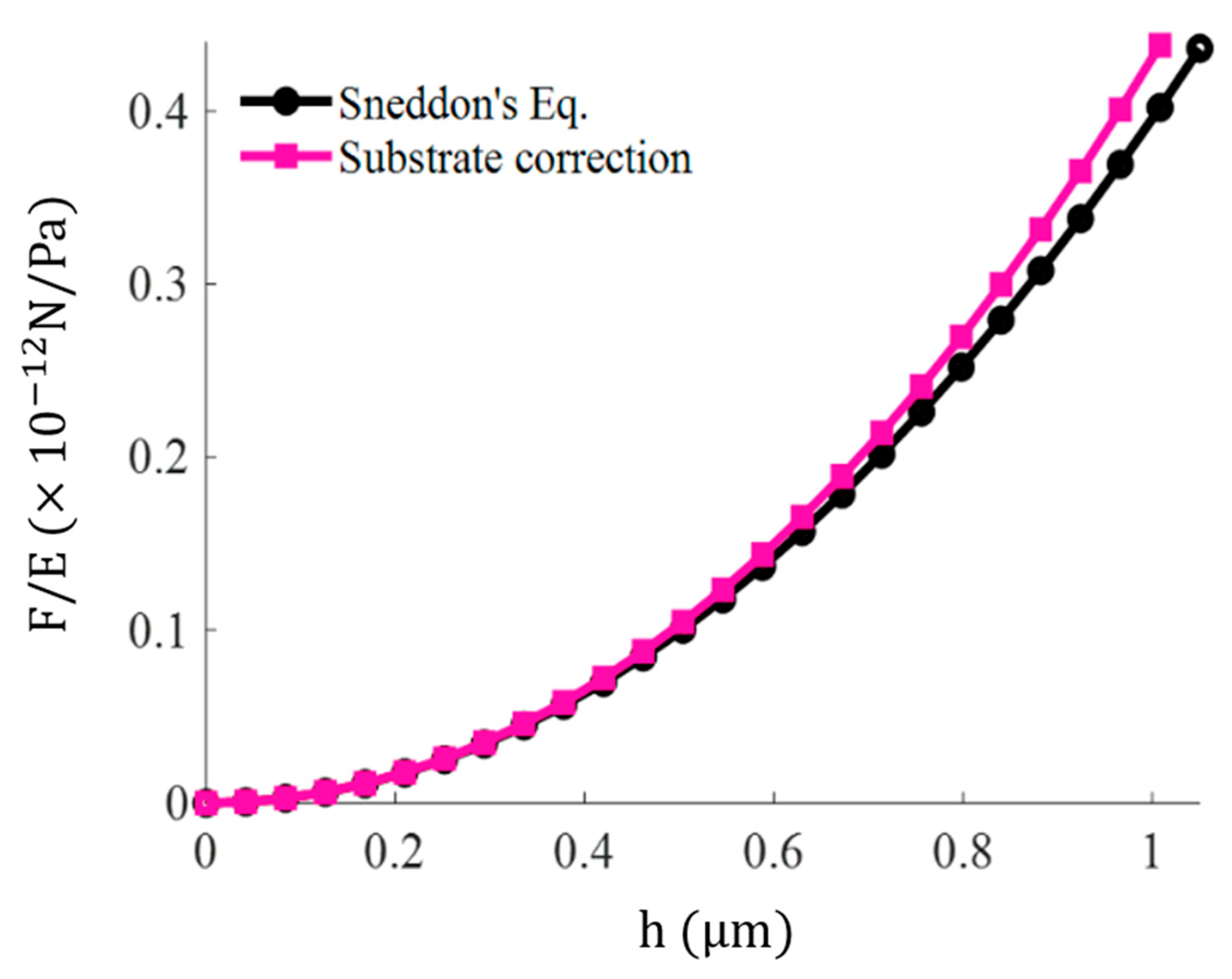
The proposed methodology can also reveal substrate effects, as shown in Figure 2, where the Young’s modulus reaches a constant value after 200–300 nm of indentation. Substrate effects would appear as a systematic change in modulus at greater depths. To avoid this, relatively small indentation depths, commonly used in the literature [7], were employed. The open-access fibroblast data [39] show a central cell height of approximately 4.2 μm. Figure 6 compares the F / E ratio (considering v = 0.5 ) obtained using Sneddon’s equation and the polynomial correction introduced by García and García [48]:
F s u b . = C S n h 2 1 + 0.721 h t a n ( θ ) H + 0.650 h 2 tan 2 ( θ ) H 2 + 0.491 h 3 tan 3 ( θ ) H 3 + 0.225 h 4 tan 4 ( θ ) H 4
The data diverge after an indentation of 800 nm, while for h < 1   μ m , the substrate effect remains minimal. Substrate effects were also negligible in the experiments with spherical indenters, where even smaller indentation depths were used (in every case < 800 nm).
An overview of the proposed method is also presented in Table 3.
An interesting question is also what differences would arise if different indenter types (e.g., conical or spherical) were used at the exact same location on the same sample. The first constant parameter, E l , represents the limiting Young’s modulus at large indentation depths. At these depths, the measured response is dominated by the bulk mechanical properties of the cell interior rather than by the local contact geometry or surface effects. Since bulk properties reflect the intrinsic stiffness of the cell, E l is expected to be largely independent of the indenter shape or size [26]. In contrast, the depth-dependent coefficient C d , which governs the variation in the modulus at shallow indentation depths, may be influenced by the initial contact geometry and therefore depends, to some extent, on the indenter. In this study, we demonstrate the existence of a universal trend describing the depth-dependent mechanical properties of cells in AFM nanoindentation experiments. Nevertheless, further research is required to quantify whether and how the generic parameter C d is affected by the contact geometry, and this will be the focus of future investigations.

5. Conclusions

In this paper, we present a new method for characterizing the depth-dependent mechanical properties of soft biological materials, along with a novel equation that captures cellular heterogeneity at any indentation depth. Using this generalized model, mechanical patterns can be derived for any heterogeneous soft sample. The new model for cells offers significant advantages, as it fully describes the mechanical behavior of a cell at a specific point using only a pair of elastic constants, C d and E l . This approach is superior to the classic Hertz–Sneddon fit for force–indentation data, which provides results that are strongly dependent on indentation depth. In addition, it offers significant advantages over more complex models, as it requires only two constants instead of complicated functional forms, providing both simplicity and physical interpretability. As a future direction, the model proposed in this paper will be applied to the analysis of experimental data obtained from normal and cancerous tissues. Since the elastic modulus can serve as a mechanical biomarker, and classical Hertzian approaches may introduce significant errors when applied to heterogeneous tissues, the proposed framework offers a viable alternative. By characterizing the tissue through a set of two elastic contact regimes, the model enables a more representative mechanical description and is expected to improve the accuracy of AFM-based diagnostic assessments.

Author Contributions

Conceptualization, S.V.K.; methodology, S.V.K., A.M., I.P. and A.S.; software, S.V.K. and A.M.; validation, S.V.K., A.M., I.P. and A.S.; investigation, S.V.K., A.M., I.P. and A.S.; resources, S.V.K., A.M., I.P. and A.S.; data curation, S.V.K.; writing—original draft preparation, S.V.K.; writing—review and editing, S.V.K., A.M., I.P. and A.S.; supervision, A.S.; project administration, S.V.K. and A.S.; funding acquisition, S.V.K. and A.S. All authors have read and agreed to the published version of the manuscript.

Funding

Funded by the European Union under the Horizon Europe’s Marie Skłodowska-Curie grant agreement No 101152646 (Project: REINFORCE). Views and opinions expressed are however those of the author(s) only and do not necessarily reflect those of the European Union or European Research Executive Agency. Neither the European Union nor the granting authority can be held responsible for them.

Data Availability Statement

All data are available within the paper.

Conflicts of Interest

Author Anna Malamou was employed by the company BioNanoTec Ltd. The remaining authors declare that the research was conducted in the absence of any commercial or financial relationships that could be construed as a potential conflict of interest.

Appendix A

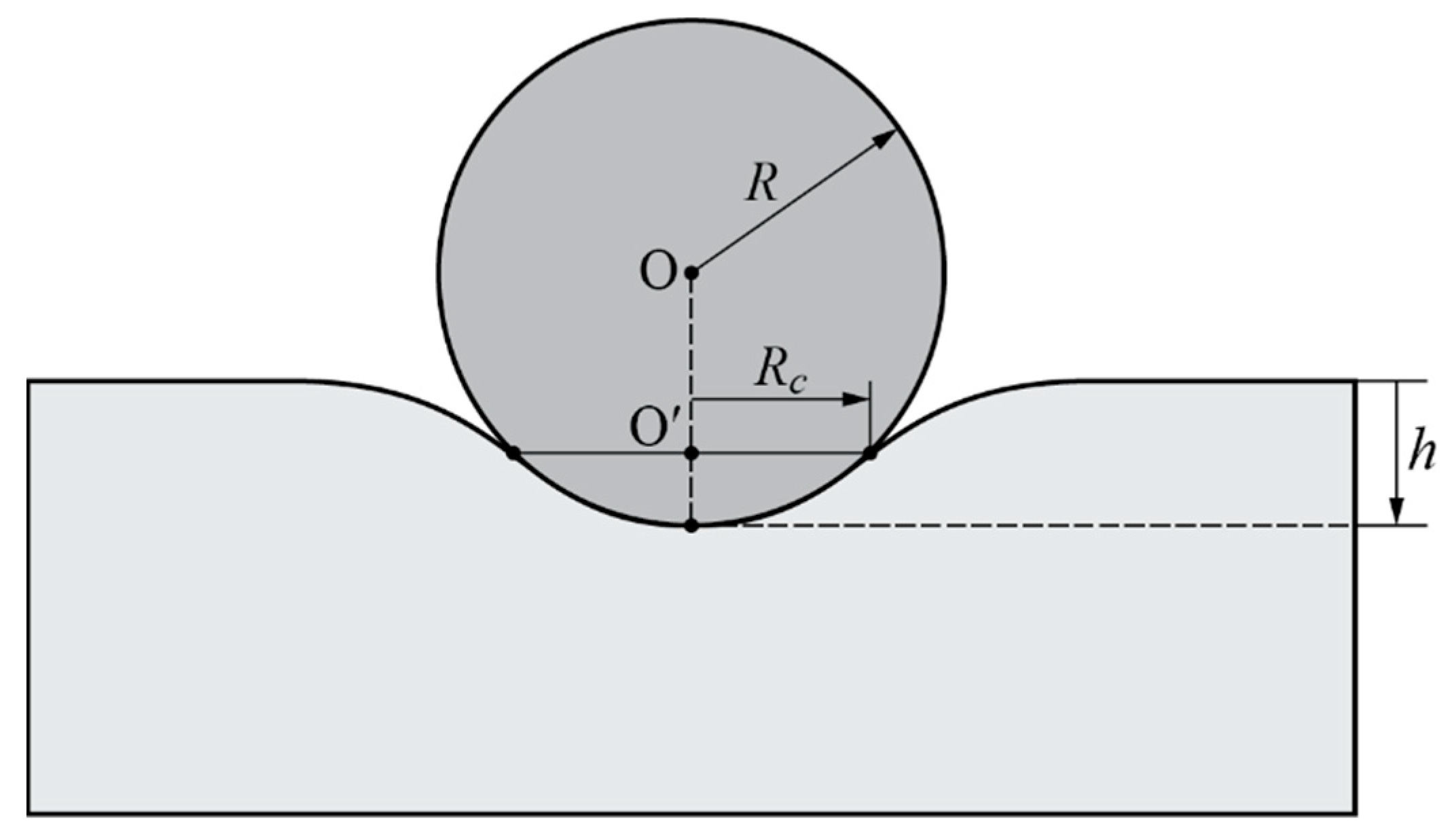
Based on the work of Sneddon [37], for a spherical punch of radius R , the indentation depth h is related to the contact radius R c (Figure A1) as follows:
h = R c 2 ln R + R c R R c
Figure A1. Deformation of elastic half space by a rigid sphere of radius R .
Eng 07 00075 g0a1
Equation (A1) can be rewritten as
h = R c 2 ln 1 + R c / R 1 R c / R = R c 2 ln 1 + R c / R ln 1 R c / R
Using a Taylor-series expansion, for the function y = ln ( 1 + x ) , x < 1 , we have
l n 1 + R c R = k = 1 1 k 1 k R c R k , 0 R c R < 1
l n 1 R c R = k = 1 1 k 1 k R c R k = k = 1 1 2 k 1 k R c R k , 0 R c R < 1
due to which
ln 1 + R c R ln 1 R c R = k = 1 1 k 1 1 1 k k R c R k , 0 R c R < 1
or:
ln 1 + R c R ln 1 R c R = 2 R c R + 2 3 R c R 3 + O R c R 5
We can introduce the approximation
ln 1 + R c R ln 1 R c R 2 R c R + 2 3 R c R 3 , R c R   
Substituting (A7) into (A2) yields
h = R c R c R + 1 3 R c R 3 = R R c R 2 + 1 3 R c R 4 1 3 R c R 4 + R c R 2 h R = 0
Let w R c R 2 0 , then (A8) is written:
1 3 w 2 + w h R = 0
with discriminant Δ = 1 + 4 3 h R > 0 , and two real roots:
w 1,2 = 3 2 1 ± Δ
Obviously, the root w 2 = 3 2 1 + Δ < 0 is rejected, leaving only one accepted root, namely
w 1 = 3 2 1 + Δ = 3 2 1 + 1 + 4 3 h R 0
where the equality on the right-hand side of the latter equation holds if and only if h = 0 . Returning to Equation (A8). we find that the only real solution is
R c R 2 = 3 2 1 + 1 + 4 3 h R     R c / R 0     R c = R 3 2 1 + 1 + 4 3 h R , R c R
At this point, it is important to note that, in most of the literature, the contact radius is typically taken as follows [58]:
R c = R h    
This equation can be easily derived from Equation (A6) by retaining only one term:
ln 1 + R c R ln 1 R c R 2 R c R
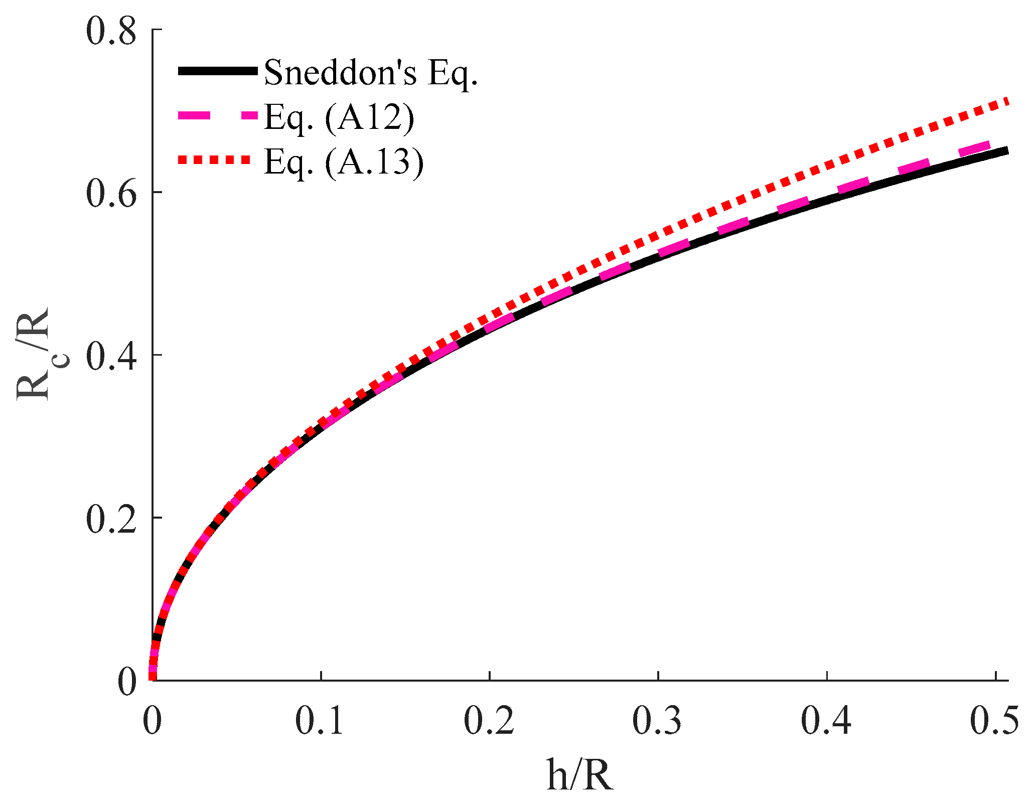
Thus, Equation (A8) is simplified as follows: h = R c 2 R R c = R h . It is generally accepted that Equation (A13), which leads to the classic Hertz equation when substituted into Equation (1), is valid only for h < R / 10 [44,45]. In Figure A2, we present the R c R = f h R plot when using Equations (A1), (A12) and (A13) for comparison. As clearly presented in Figure A2, the contact radius equation proposed in this paper (i.e., Equation (A12)) can be applied over a much wider range of indentation depths.
Figure A2. The R c / R versus h / R plots obtained using Sneddon’s equation (Equation (A1)), the proposed by this paper approach (Equation (A12)) and the parabolic approximation (Equation (A13)).
Eng 07 00075 g0a2

References

  1. Lekka, M.; Laidler, P. Applicability of AFM in cancer detection. Nat. Nanotechnol. 2009, 4, 72. [Google Scholar] [CrossRef] [PubMed]
  2. Plodinec, M.; Loparic, M.; Monnier, C.A.; Obermann, E.C.; Zanetti-Dallenbach, R.; Oertle, P.; Hyotyla, J.T.; Aebi, U.; Bentires-Alj, M.; Lim, R.Y.H.; et al. The nanomechanical signature of breast cancer. Nat. Nanotechnol. 2012, 7, 757–765. [Google Scholar] [CrossRef]
  3. Stylianou, A.; Lekka, M.; Stylianopoulos, T. AFM assessing of nanomechanical fingerprints for cancer early diagnosis and classification: From single cell to tissue level. Nanoscale 2018, 10, 20930–20945. [Google Scholar] [CrossRef]
  4. Lei, C.; Shao, W.; Yuan, X.; Xu, L.; Tuzikov, A.; Sabirov, R.; Calamak, S.; Varol, H.A.; Sajjad, N.; Qin, P. Regional variations in mechanical properties of porcine leptomeninges. Cyborg Bionic Syst. 2025, 6, 0462. [Google Scholar] [CrossRef]
  5. Stylianou, A.; Voutouri, C.; Mpekris, F.; Stylianopoulos, T. Pancreatic Cancer Presents Distinct Nanomechanical Properties During Progression. Ann. Biomed. Eng. 2023, 51, 1602–1615. [Google Scholar] [CrossRef]
  6. Lekka, M.; Gil, D.; Pogoda, K.; Dulińska-Litewka, J.; Jach, R.; Gostek, J.; Laidler, P. Cancer cell detection in tissue sections using AFM. Arch. Biochem. Biophys. 2012, 518, 151–156. [Google Scholar] [CrossRef]
  7. Lekka, M. Discrimination between normal and cancerous cells using AFM. BioNanoScience 2016, 6, 65–80. [Google Scholar] [CrossRef] [PubMed]
  8. Zemła, J.; Danilkiewicz, J.; Orzechowska, B.; Pabijan, J.; Seweryn, S.; Lekka, M. Atomic force microscopy as a tool for assessing the cellular elasticity and adhesiveness to identify cancer cells and tissues. Semin. Cell Dev. Biol. 2018, 73, 115–124. [Google Scholar] [CrossRef] [PubMed]
  9. Cross, S.E.; Jin, Y.-S.; Tondre, J.; Wong, R.; Rao, J.; Gimzewski, J.K. AFM-based analysis of human metastatic cancer cells. Nanotechnology 2008, 19, 385102. [Google Scholar] [CrossRef]
  10. Magazzù, A.; Marcuello, C. Investigation of Soft Matter Nanomechanics by Atomic Force Microscopy and Optical Tweezers: A Comprehensive Review. Nanomaterials 2023, 13, 963. [Google Scholar] [CrossRef]
  11. Filippi, J.; Casti, P.; Lacconi, V.; Antonelli, G.; D’Orazio, M.; Curci, G.; Ticconi, C.; Rago, R.; De Luca, M.; Martinelli, E. ODEP-based robotic system for micromanipulation and in-flow analysis of primary cells. Cyborg Bionic Syst. 2025, 6, 0234. [Google Scholar] [CrossRef]
  12. Baradaran Najar, A.; Gilbert, G.; Li, N.; He, Z.; Ghazavi, S.; Nguyen, B.N.; Fohlen, A.; Cloutier, G.; Tang, A.; Van Houten, E. Wide-band multifrequency MR elastography with a fractional viscoelastic model and nonlinear inversion for enhanced viscoelastic parameter mapping. Acta Biomater. 2025, 208, 386–401. [Google Scholar] [CrossRef]
  13. Wenger, M.P.; Bozec, L.; Horton, M.A.; Mesquida, P. Mechanical properties of collagen fibrils. Biophys. J. 2007, 93, 1255–1263. [Google Scholar] [CrossRef]
  14. Rodenburg, W.S.; Ebben, S.F.A.; Eeftens, J.M. Robust quantification of cellular mechanics using optical tweezers. Biophys. Rep. 2025, 5, 100199. [Google Scholar] [CrossRef]
  15. Lekka, M.; Laidler, P.; Gil, D.; Lekki, J.; Stachura, Z.; Hrynkiewicz, A.Z. Elasticity of normal and cancerous human bladder cells studied by scanning force microscopy. Eur. Biophys. J. 1999, 28, 312–316. [Google Scholar] [CrossRef]
  16. Holuigue, H.; Lorenc, E.; Chighizola, M.; Schulte, C.; Varinelli, L.; Deraco, M.; Guaglio, M.; Gariboldi, M.; Podestà, A. Force sensing on cells and tissues by atomic force microscopy. Sensors 2022, 22, 2197. [Google Scholar] [CrossRef]
  17. Hayashi, K.; Iwata, M. Stiffness of cancer cells measured with an AFM indentation method. J. Mech. Behav. Biomed. Mater. 2015, 49, 105–111. [Google Scholar] [CrossRef] [PubMed]
  18. Viji Babu, P.K.; Radmacher, M. Mechanics of brain tissues studied by atomic force microscopy: A perspective. Front. Neurosci. 2019, 13, 600. [Google Scholar] [CrossRef] [PubMed]
  19. Liu, S.; Han, Y.; Kong, L.; Wang, G.; Ye, Z. Atomic force microscopy in disease-related studies: Exploring tissue and cell mechanics. Microsc. Res. Tech. 2023, 87, 660–684. [Google Scholar] [CrossRef] [PubMed]
  20. Zhou, G.; Zhang, B.; Tang, G.; Yu, X.F.; Galluzzi, M. Cells nanomechanics by atomic force microscopy: Focus on interactions at the nanoscale. Adv. Phys. X 2021, 6, 1. [Google Scholar] [CrossRef]
  21. Liang, W.; Shi, H.; Yang, X.; Wang, J.; Yang, W.; Zhang, H.; Liu, L. Recent advances in AFM-based biological characterizations and applications at multiple levels. Soft Matter 2020, 16, 8962–8984. [Google Scholar] [CrossRef] [PubMed]
  22. Stolz, M.; Gottardi, R.; Raiteri, R.; Miot, S.; Martin, I.; Imer, R.; Staufer, U.; Raducanu, A.; Düggelin, M.; Baschong, W.; et al. Early detection of aging cartilage and osteoarthritis in mice and patient samples using atomic force microscopy. Nat. Nanotechnol. 2009, 4, 186–192. [Google Scholar] [CrossRef]
  23. Schillers, H.; Rianna, C.; Schape, J.; Luque, T.; Doschke, H.; Wälte, M.; Uriarte, J.J.; Campillo, N.; Michanetzis, G.P.A.; Bobrowska, J.; et al. Standardized nanomechanical atomic force microscopy procedure (SNAP) for measuring soft and biological samples. Sci. Rep. 2017, 7, 5117. [Google Scholar] [CrossRef]
  24. Krieg, M.; Flaschner, G.; Alsteens, D.; Gaub, B.M.; Roos, W.H.; Wuite, G.J.L.; Gaub, H.E.; Gerber, C.; Dufrêne, Y.F.; Müller, D.J. Atomic force microscopy-based mechanobiology. Nat. Rev. Phys. 2019, 1, 41–57. [Google Scholar] [CrossRef]
  25. Pogoda, K.; Jaczewska, J.; Wiltowska-Zuber, J.; Klymenko, O.; Zuber, K.; Fornal, M.; Lekka, M. Depth-sensing analysis of cytoskeleton organization based on AFM data. Eur. Biophys. J. 2012, 41, 79–87. [Google Scholar] [CrossRef] [PubMed]
  26. Ding, Y.; Wang, J.; Xu, G.K.; Wang, G.F. Are elastic moduli of biological cells depth dependent or not? Another explanation using a contact mechanics model with surface tension. Soft Matter 2018, 14, 7534–7541. [Google Scholar] [CrossRef]
  27. Kontomaris, S.V.; Georgakopoulos, A.; Malamou, A.; Stylianou, A. The average Young’s modulus as a physical quantity for describing the depth-dependent mechanical properties of cells. Mech. Mater. 2021, 158, 103846. [Google Scholar] [CrossRef]
  28. Amo, C.A.; Perrino, A.P.; Payam, A.F.; Garcia, R. Mapping elastic properties of heterogeneous materials in liquid with angstrom-scale resolution. ACS Nano 2017, 11, 8650–8659. [Google Scholar] [CrossRef]
  29. Doss, B.L.; Rahmani Eliato, K.; Lind, K.H.; Ros, R. Quantitative mechanical analysis of indentations on layered, soft elastic materials. Soft Matter 2019, 15, 1776–1784. [Google Scholar] [CrossRef]
  30. Chen, S.W.; Teulon, J.-M.; Kaur, H.; Godon, C.; Pellequer, J.-L. Nano-structural stiffness measure for soft biomaterials of heterogeneous elasticity. Nanoscale Horiz. 2023, 8, 75–82. [Google Scholar] [CrossRef] [PubMed]
  31. Kontomaris, S.V.; Stylianou, A.; Georgakopoulos, A.; Malamou, A. 3D AFM nanomechanical characterization of biological materials. Nanomaterials 2023, 13, 395. [Google Scholar] [CrossRef]
  32. Kontomaris, S.V.; Stylianou, A.; Chliveros, G.; Malamou, A. AFM indentation on highly heterogeneous materials using different indenter geometries. Appl. Mech. 2023, 4, 460–475. [Google Scholar] [CrossRef]
  33. Pharr, G.M.; Oliver, W.C.; Brotzen, F.R. On the generality of the relationship among contact stiffness, contact area, and elastic properties of materials. J. Mater. Res. 1992, 7, 613–617. [Google Scholar] [CrossRef]
  34. Khan, A.; Philip, J.; Hess, P. Young’s modulus of silicon nitride used in scanning force microscope cantilevers. J. Appl. Phys. 2004, 95, 1667–1672. [Google Scholar] [CrossRef]
  35. Kontomaris, S.V.; Stylianou, A.; Georgakopoulos, A.; Malamou, A. Is it mathematically correct to fit AFM data (obtained on biological materials) to equations arising from Hertzian mechanics? Micron 2023, 164, 103384. [Google Scholar] [CrossRef]
  36. Kontomaris, S.V.; Malamou, A. Hertz model or Oliver & Pharr analysis? Tutorial regarding AFM nanoindentation experiments on biological samples. Mater. Res. Express 2020, 7, 033001. [Google Scholar] [CrossRef]
  37. Sneddon, I.N. The relation between load and penetration in the axisymmetric Boussinesq problem for a punch of arbitrary profile. Int. J. Eng. Sci. 1965, 3, 47–57. [Google Scholar] [CrossRef]
  38. Puricelli, L.; Galluzzi, M.; Schulte, C.; Podestà, A.; Milani, P. Nanomechanical and topographical imaging of living cells by atomic force microscopy with colloidal probes. Rev. Sci. Instrum. 2015, 86, 033705. [Google Scholar] [CrossRef] [PubMed]
  39. Hermanowicz, P.; Sarna, M.; Burda, K.; Gabryś, H. AtomicJ: An open-source software for analysis of force curves. Rev. Sci. Instrum. 2014, 85, 063703. [Google Scholar] [CrossRef]
  40. Kontomaris, S.V.; Stylianou, A.; Nikita, K.S.; Malamou, A. Determination of the linear elastic regime in AFM nanoindentation experiments on cells. Mater. Res. Express 2019, 6, 115410. [Google Scholar] [CrossRef]
  41. Kontomaris, S.-V.; Malamou, A.; Ismail, G.M.; Katsiki, A.; Stylianou, A. Beyond Hertz: Accurate Analytical Force–Indentation Equations for AFM Nanoindentation with Spherical Tips. Metrology 2025, 5, 63. [Google Scholar] [CrossRef]
  42. Wang, B.; Lançon, P.; Bienvenu, C.; Vierling, P.; Di Giorgio, C.; Bossis, G. A general approach for the microrheology of cancer cells by atomic force microscopy. Micron 2013, 44, 287–297. [Google Scholar] [CrossRef]
  43. Müller, P.; Abuhattum, S.; Möllmert, S.; Ulbricht, E.; Taubenberger, A.V.; Guck, J. nanite: Using machine learning to assess the quality of atomic force microscopy-enabled nano-indentation data. BMC Bioinform. 2019, 20, 465. [Google Scholar] [CrossRef]
  44. Wu, C.-E.; Lin, K.-H.; Juang, J.-Y. Hertzian Load–Displacement Relation Holds for Spherical Indentation on Soft Elastic Solids Undergoing Large Deformations. Tribol. Int. 2016, 97, 71–76. [Google Scholar] [CrossRef]
  45. Koruk, H.; Pouliopoulos, A.N. Elasticity and Viscoelasticity Imaging Based on Small Particles Exposed to External Forces. Processes 2023, 11, 3402. [Google Scholar] [CrossRef]
  46. Dimitriadis, E.K.; Horkay, F.; Maresca, J.; Kachar, B.; Chadwick, R.S. Determination of elastic moduli of thin layers of soft material using AFM. Biophys. J. 2002, 82, 2798–2810. [Google Scholar] [CrossRef] [PubMed]
  47. Gavara, N.; Chadwick, R.S. Determination of elastic moduli of thin samples and adherent cells using conical AFM tips. Nat. Nanotechnol. 2012, 7, 733–736. [Google Scholar] [CrossRef] [PubMed]
  48. Garcia, P.D.; Garcia, R. Determination of elastic moduli of a single cell cultured on a rigid support by force microscopy. Biophys. J. 2018, 114, 2923–2932. [Google Scholar] [CrossRef] [PubMed]
  49. Gavara, N. A beginner’s guide to atomic force microscopy probing for cell mechanics. Microsc. Res. Tech. 2017, 80, 75–84. [Google Scholar] [CrossRef]
  50. Guz, N.; Dokukin, M.; Kalaparthi, V.; Sokolov, I. If cell mechanics can be described by elastic modulus: Study of different models and probes used in indentation experiments. Biophys. J. 2014, 107, 564–575. [Google Scholar] [CrossRef]
  51. Yang, N.; Wong, K.K.H.; de Bruyn, J.R.; Hutter, J.L. Frequency-Dependent Viscoelasticity Measurement by Atomic Force Microscopy. Meas. Sci. Technol. 2009, 20, 025703. [Google Scholar] [CrossRef]
  52. Hinterdorfer, P.; Dufrêne, Y.F. Detection and localization of single molecular recognition events using atomic force microscopy. Nat. Methods 2006, 3, 347–355. [Google Scholar] [CrossRef]
  53. Chen, X.; Li, B.; Liao, Z.; Li, J.; Li, X.; Yin, J.; Guo, W. Principles and applications of liquid-environment atomic force microscopy. Adv. Mater. Interfaces 2022, 9, 2201864. [Google Scholar] [CrossRef]
  54. Wei, Z.; Zhao, Y.P. Growth of liquid bridge in AFM. J. Phys. D Appl. Phys. 2007, 40, 4368–4375. [Google Scholar] [CrossRef]
  55. Dokukin, M.E.; Guz, N.V.; Sokolov, I. Quantitative study of the elastic modulus of loosely attached cells in AFM indentation experiments. Biophys. J. 2013, 104, 2123–2131. [Google Scholar] [CrossRef] [PubMed]
  56. Oliver, W.C.; Pharr, G.M. Measurement of hardness and elastic modulus by instrumented indentation: Advances in understanding and refinements to methodology. J. Mater. Res. 2004, 19, 3–20. [Google Scholar] [CrossRef]
  57. Kontomaris, S.V.; Malamou, A.; Stylianou, A. The Hertzian theory in AFM nanoindentation experiments regarding biological samples: Overcoming limitations in data processing. Micron 2022, 155, 103228. [Google Scholar] [CrossRef]
  58. Popov, V.L.; Heß, M.; Willert, E. Handbook of Contact Mechanics: Exact Solutions of Axisymmetric Contact Problems, 1st ed.; Springer: Cham, Switzerland, 2019. [Google Scholar]
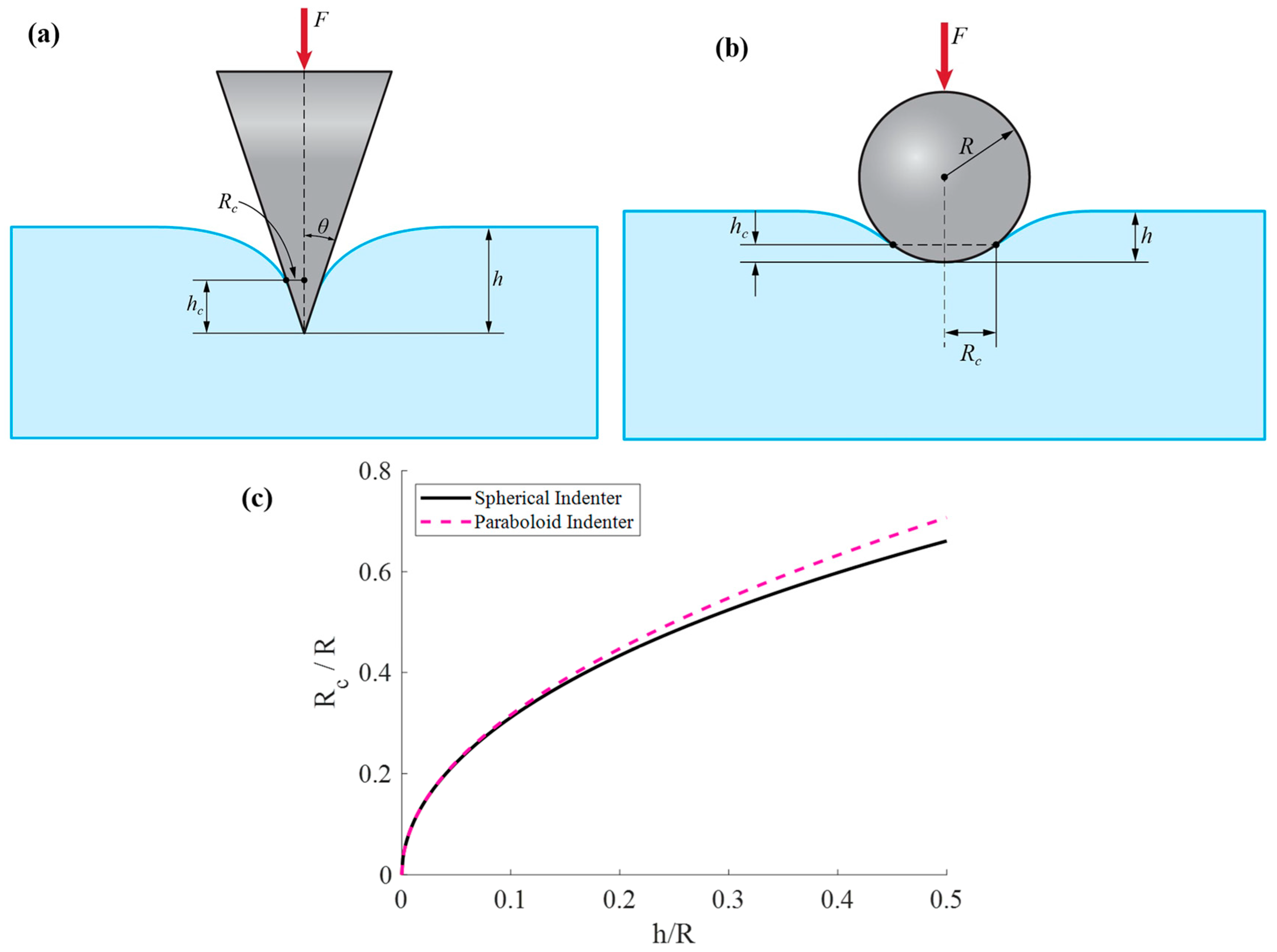
Figure 1. (a) Indentation using a conical indenter. (b) Indentation using a spherical indenter. The contact radius is presented in both cases. (c) Comparison of the normalized contact radius R c / R as a function of the normalized indentation depth h / R for a spherical indenter (Equation (10)) and the parabolic approximation (Equation (12)). For small indentation depths ( h R ), both approaches converge, yielding identical results as expected.
Eng 07 00075 g001
Figure 2. Three representative force–indentation curves obtained from fibroblasts are shown in panels (aiaiii). The elastic modulus at each indentation depth was calculated using Equation (8), and the resulting depth-dependent modulus curves, E = f ( h ) , are presented in panels (bibiii). These plots illustrate the variation in the apparent modulus with indentation depth for different mechanical behaviors observed in the cells.
Eng 07 00075 g002
Figure 3. (ai) Bar charts of the R-squared coefficients for the 4th-degree polynomial fit and the Sneddon fit, including error bars. The mean ± standard deviation values were 0.99955 ± 0.00073 for the polynomial fit and 0.97812 ± 0.01520 for the Sneddon fit, indicating higher consistency and accuracy of the polynomial fitting approach. (aii,aiii) Histograms of the stiffness coefficient C d and limiting modulus E l with Gaussian fits; the mean ± standard deviation values are C d = ( 1.40 ± 0.26 ) × 10 3 N/m and E l = 3.76 ± 1.46 kPa. (bi,bii) Distributions of E m e a n and E S n , corresponding to the mean modulus from the proposed model (Equation (17)) and the Sneddon fit, with mean ± standard deviation values of E m e a n = 7.46 ± 1.80 kPa and E S n = 7.51 ± 1.95 kPa. (biii) Comparison of the Gaussian fits for E m e a n and E S n , demonstrating that the proposed method can also produce the results of the classic Sneddon fit.
Eng 07 00075 g003
Figure 4. A representative force–indentation curve obtained from a H4 human glioma cell is shown in panel (a). The elastic modulus at each indentation depth was calculated using Equation (11), and the resulting depth-dependent modulus curve, E = f ( h ) , is presented in panel (b).
Eng 07 00075 g004
Figure 5. (ai) Bar charts of the R s . c . 2 for the fourth-degree polynomial and Hertzian fits, including error bars. The mean ± standard deviation values were 0.99989 ± 0.00008 for the polynomial fit and 0.99119 ± 0.0055 for the Hertzian fit. (aii,aiii) Histograms of the stiffness coefficient C d and limiting modulus E l with Gaussian fits; the mean ± standard deviation values are C d = ( 1.88 ± 0.49 ) × 10 4 N/m and E l = 4.75 ± 1.79 kPa. (bi,bii) Distributions of E mean and E Hertz , corresponding to the mean modulus from the proposed model (Equation (17)) and the Hertzian fit (Equation (18)), with mean ± standard deviation values of E mean = 5.70 ± 1.99 kPa and E Hertz = 5.53 ± 1.87 kPa. (biii) Comparison of the Gaussian fits for E mean and E Hertz .
Eng 07 00075 g005
Figure 6. Comparison between the classic Sneddon equation for a perfect conical indenter acting on an elastic half-space and the Garcia and Garcia equation (Equation (19)), which accounts for the presence of a rigid substrate when testing a cell. The cell height was assumed to be 4.2 μm, and the Poisson’s ratio was v = 0.5 .
Eng 07 00075 g006
Table 1. Conical indenter: Summary of fitting results for fibroblast force–indentation measurements. The first two columns show R-squared coefficients for the 4th-degree polynomial fit and the classic Sneddon fit. Columns three and four report the depth-dependent stiffness coefficient C d (×10−3 N/m) and the limiting apparent modulus E l (kPa), respectively. Column five presents the R-squared coefficients values for the cell mechanics model fit using Equation (14). Columns six and seven compare the mean modulus E m e a n , calculated from the cell model (Equation (17)), with the modulus obtained from the Sneddon fit E S n . This table demonstrates that the proposed cell mechanics model accurately captures the depth-dependent mechanical behavior of fibroblasts while remaining consistent with conventional Sneddon-based analysis.
R s . c . ( p o l y n . f i t . ) 2 R s . c . ( S n e d . f i t . ) 2 C d
× 10 3 N m
E l
K P a
R s . c . ( c e l l   m o d e l . ) 2 E m e a n
K P a
E S n
K P a
0.999900.989591.373.340.986096.77 6.76
0.999690.928312.091.420.997366.94 6.91
0.999740.961911.152.380.999444.99 4.91
0.999840.960831.342.700.998866.01 6.00
0.999780.966171.302.930.998656.15 6.15
0.999800.986081.254.880.994558.25 8.38
0.999670.972671.777.790.9985213.58 14.28
0.999830.988281.253.470.991066.58 6.58
0.999770.973281.352.530.996215.75 5.69
0.999750.975991.304.110.998307.46 7.54
0.999680.970291.533.990.997828.08 8.21
0.999780.960831.523.040.998456.93 6.96
0.999780.967551.433.530.998787.14 7.17
0.999760.982081.164.000.997356.90 6.94
0.999780.971671.282.620.997325.66 5.62
0.999720.957352.053.630.997159.31 9.71
0.999950.980911.293.150.994806.37 6.38
0.999900.996740.935.960.977258.56 8.63
0.999870.980221.383.710.994987.28 7.34
0.999850.989941.277.330.9926411.17 11.49
0.999810.990921.514.540.980588.78 8.88
0.997830.984161.532.600.952076.74 6.67
0.999670.993911.163.890.970646.96 6.96
0.999580.991691.112.840.961265.63 5.56
0.999730.993491.415.170.959519.23 9.28
0.999580.991691.112.840.961265.635.56
0.999730.993491.415.170.959519.23 9.28
0.999640.990881.304.330.945167.93 7.86
0.996300.965341.881.430.938816.27 6.01
0.998840.987241.483.520.947807.59 7.50
Table 2. Spherical indenter: Summary of the fitting results for the force–indentation measurements on a H4 human glioma cell. The first two columns show R-squared coefficients for the 4th-degree polynomial fit and the Hertzian fit for large indentations (Equation (18)). Columns three and four report the stiffness coefficient C d ( × 10 4   N / m ) and the limiting apparent modulus E l , respectively. Column five presents the R-squared coefficients values for the cell mechanics model fit using Equation (14). Columns six and seven compare the mean modulus E m e a n , calculated from the cell model, with the modulus obtained from the extended Hertzian fit (i.e., through Equation (18)).
R s . c . ( p o l y n . f i t . ) 2
R s . c . ( H e r t z   f i t . ) 2
C d × 10 4 N m
E l K P a
R s . c . ( c e l l   m o d e l . ) 2
E m e a n K P a
E H e r t z K P a
0.999950.982191.803.610.972694.544.48
0.999870.986101.953.450.964284.454.27
0.999960.993871.203.600.993594.214.16
0.999960.988161.753.570.980784.474.34
0.999800.997101.023.670.923674.184.08
0.999830.992501.323.680.990214.354.31
0.999910.991732.004.930.986445.945.82
0.999980.992721.143.180.990093.753.72
0.999790.992881.413.640.978764.374.26
0.999960.987351.753.610.985404.514.41
0.999940.993991.473.960.978334.704.60
0.999940.994571.413.920.967524.654.53
0.999960.992371.673.950.972294.794.65
0.999900.992912.055.010.965206.045.86
0.999880.978172.003.170.977494.154.10
0.999960.974251.962.890.972283.853.80
0.999910.991141.874.320.981815.285.14
0.999930.993781.673.940.894204.784.56
0.999860.996072.417.010.878688.217.90
0.999720.996472.538.020.870149.278.94
0.999720.996982.127.210.918678.278.05
0.999730.997492.168.330.807399.419.08
0.999870.995882.919.060.7257110.529.95
0.999960.985351.673.190.983504.033.93
0.999920.989972.334.960.974606.145.95
0.999880.993042.235.350.949056.496.27
0.999990.993842.375.980.952677.186.95
0.999990.992321.303.300.985023.963.88
0.999930.987631.884.010.985314.974.87
0.999810.994853.058.000.880639.529.12
Table 3. A summary of the proposed method for characterizing soft heterogeneous samples using AFM nanoindentation, with particular emphasis on the special case of cells.
A Generalized Method for Heterogeneous Soft Materials

1st Step: A 4th degree polynomial fit
Eng 07 00075 i001
F = c 1 h + c 2 h 2 + c 3 h 3 + c 4 h 4


2nd Step: Calculating the E = f ( h ) data
Eng 07 00075 i002


For conical indenters:

E c o n e ( h ) = 3 π 16 tan θ h n = 1 4 n c n h n 1

For spherical indenters:

E s p h e r e ( h ) = 3 8 R 3 2 1 + 1 + 4 3 h R n = 1 m n c n h n 1
The special case of cells
  • Fit the E = f ( h ) data to E h = C d h + E l
  • Obtain a pair of constants, C d and E l , to fully describe the cell’s heterogeneity at any indentation depth.
Disclaimer/Publisher’s Note: The statements, opinions and data contained in all publications are solely those of the individual author(s) and contributor(s) and not of MDPI and/or the editor(s). MDPI and/or the editor(s) disclaim responsibility for any injury to people or property resulting from any ideas, methods, instructions or products referred to in the content.