Article

Localized Reluctivity Stabilization of Hysteresis Model for Transient Finite Element Simulation of Ferromagnetic Materials

1
State Key Laboratory of High Density Electromagnetic Power and Systems, Institute of Electrical Engineering, Chinese Academy of Sciences, Beijing 100190, China
2
University of Chinese Academy of Sciences, Beijing 101408, China
3
Laboratoire de Génie Electrique et Electronique de Paris, GeePs, Sorbonne Université, CNRS, 75005 Paris, France
*
Author to whom correspondence should be addressed.
Eng 2025, 6(11), 289; https://doi.org/10.3390/eng6110289
Submission received: 7 October 2025 / Revised: 24 October 2025 / Accepted: 27 October 2025 / Published: 28 October 2025
(This article belongs to the Special Issue Interdisciplinary Insights in Engineering Research)

Abstract

The hysteresis model can be used to accurately predict the magnetic hysteresis characteristics of ferromagnetic materials. Incorporating the hysteresis model into finite element calculations enables precise prediction of field distributions, voltage or current variations in circuits, and losses, which is essential for electromagnetic transient analysis involving remanent magnetization. When incorporating the hysteresis model into finite element analysis, prohibitively small time-steps are required to resolve hysteresis loops, leading to excessive simulation times compared to simplified BH curve approaches. Furthermore, numerical instabilities arise near zero-crossing points of magnetic flux density, where erroneous negative differential reluctivity values may lead to the divergence of the nonlinear solving process. A finer time resolution needs to be utilized to ensure the convergence of the nonlinear solver. This leads to more time-steps and longer computational time. This work proposes a localized stabilization strategy for regulating the differential reluctivity in instability-prone regions of the hysteresis loop, which can stabilize the nonlinear iteration while avoiding the local refinement of time resolution and thus reduce the overall computation time.

1. Introduction

Ferromagnetic materials play a critical role in electrical equipment such as motors and transformers by enabling efficient energy transfer. Accurate fitting of the hysteresis characteristics of ferromagnetic materials is essential for both optimal design and safe operation of electrical equipment. The BH curve is conventionally employed for the characterization of nonlinear material properties of ferromagnetic materials in finite element analysis. However, it fails to account for hysteresis phenomena and cannot directly calculate the core loss. This limitation becomes particularly evident in transient analysis scenarios. For instance, when investigating the inrush current of a transformer, which is intrinsically linked to remanent magnetization, the hysteresis model must be considered [1,2], as the BH curve cannot capture the remanence-related effects.
In order to accurately describe the hysteresis characteristics of ferromagnetic materials, a variety of hysteresis models have been developed. The Jiles–Atherton (JA) model and Preisach model are the two most widely used hysteresis models [3,4]. Among them, the JA model has the advantages of clearer physical meaning, less model parameters, and easier implementation. Therefore, in this work, we utilize the JA model for hysteresis modeling. The JA model was first introduced in [3]. The original JA model is a scalar model, which is only applicable to the case where the magnetic field is unidirectional and material properties are isotropic, lacking the capability to describe vector hysteresis phenomena or anisotropic magnetic behavior. Based on the original JA model [3], researchers have proposed a variety of modified versions [5,6,7,8] in order to apply to a wider range of application scenarios. Sadowski et al. first proposed the inverse JA scalar model [5], which is only applicable to the case where the field changes in a single direction. In fact, the field in the iron core of most applications is rotating, especially in the T-shaped area of the transformer core or the stator yoke of the rotating motor, which should be solved by the vector JA model. Bergqvist et al. [6] first proposed the vector JA model, which can be applied to anisotropic materials. Later, Leite et al. proposed the inverse vector JA model [7], and reference [8] proposed the modified vector JA model, adding off-diagonal reluctivity parameters to improve the calculation accuracy.
Finite element analysis incorporating the hysteresis model faces two major computational challenges: computational cost and convergence problems. First, the computation time of finite element calculation when considering the hysteresis model increases significantly. This is because the time-step required by the hysteresis model is several times smaller than the case of linear or single-valued BH curves. Second, the convergence is seriously degraded due to the difference in the variation rate of reluctivity at different parts of the hysteresis loop. Numerical convergence issues frequently emerge near the zero-crossing region of the magnetic flux density (B-field) on hysteresis loops, where the magnetic flux density exhibits a sharp change and the differential reluctivity approaches its minimum. Large time-steps in this critical region may induce non-physical negative differential reluctivity values, ultimately causing the divergence of the nonlinear iterations. Local refinement of the temporal resolution near the B-field zero-crossing regions can stabilize the iterations. Reference [9] proposed to use the differential reluctivity of the previous time-step when the negative differential reluctivity appears to avoid convergence issues. The calculation results of actual numerical examples show that the stabilization algorithm in [9] may cause the differential reluctivity rate to remain unchanged for several consecutive time-steps. The calculated hysteresis loop will change linearly at different stages, which may have a large error with the actual hysteresis loop. It is not easy to determine the threshold value of the stabilization algorithm. If it is set too high, the differential reluctivity rate after stabilization will still not be smooth enough, and if it is set too low, the calculation efficiency cannot be effectively improved.
In our work, it is observed from the hysteresis loop that near the zero-crossing region of the magnetic flux density, there exists a local asymptotic symmetry on the differential reluctivity. This property can ultimately be used to improve the calculation efficiency and accuracy at the same time. Based on this, in this paper, a localized differential reluctivity stabilization method is proposed. The method is used in a finite element transient analysis where both the scalar and vector JA hysteresis models are incorporated. The differential reluctivity of the B-field at the zero-crossing region is guaranteed to be non-negative, so that the nonlinear iterations can be stabilized without a refinement of the temporal resolution, and thus the computational overhead can be effectively avoided.
The remainder of the paper is organized as follows: In Section 2, the definition of the JA model is summarized, and the field equations considering the JA model are introduced. In Section 3, a local stability algorithm of differential reluctivity is proposed. Finally, in Section 4, a 2-D numerical example is chosen to verify the effectiveness of the proposed method.

2. JA Model and Field Equations

2.1. Scalar JA Model

The JA hysteresis model divides the magnetization in actual materials into reversible magnetization and irreversible magnetization, which are recorded as Mrev and Mirr, respectively, and only irreversible magnetization can produce hysteresis effect. The non-hysteresis magnetization intensity Man is defined as shown in (1).
M a n = M s ( c o t h H + α M a a H + α M )
where Ms is the saturation magnetization, α is the average field coefficient of the internal coupling of the magnetic domain, a is the shape parameter of the non-hysteresis magnetization curve, H is the magnetic field intensity, and Man is the magnetization intensity generated by the ideal material magnetization without a hysteresis effect. The energy balance equation is established according to the principle of internal energy conservation of the material. The static magnetic energy generated by the non-hysteresis magnetization of the material in the ideal state is equal to the sum of the static magnetic energy of the actual material magnetization and the hysteresis loss caused by the pinning point in the actual magnetization process, as shown in (2):
μ 0 M a n d H e = μ 0 M d H e + μ 0 k δ ( 1 c ) d M i r r d M H e d H e
where k is the pinning coefficient; c is the reversible magnetization coefficient, and δ is the direction coefficient; when dH/dt > 0, δ = 1, and when dH/dt <= 0, δ = −1. This is to ensure that the blocking effect of the pinning point is opposite to the direction of the magnetic field change. μ0 is the relative permeability of vacuum, M is the actual magnetization, He is the effective magnetic field strength, and He = H + αMan. Equation (2) can be simplified as follows:
d M i r r d H e = M a n M i r r k δ
To prevent non-physics results, reference [6] suggested rewriting (3) as
d M i r r = 1 k δ [ M a n M i r r d H e ] +
where the notation [x]+ means that when x > 0, [x]+ = x; otherwise, [x]+ = 0. And because
d M r e v = c ( d M a n d M i r r )
the differential of total magnetization can be obtained:
d M = 1 k δ [ M a n M d H e ] + + c d M a n
Equation (6) is the differential expression of the JA model.
Equation (6) is called the direct JA model, where the magnetization M is a function of H . By expressing M as a function of B , the inverse JA model can be obtained, as shown in (7):
d M = 1 k δ ( M a n M ) d B μ 0 + + c d M a n 1 1 k δ ( M a n M ) ( α 1 )
where Be is the effective magnetic flux density, and Be = μ0He.

2.2. Improved Vector JA Model

Reference [6] proposed a simple vector model, which extends the scalar JA model dM = f (B, M, H) to dM = f (B, M, H); that is,
d M = χ f χ f 1 · χ f · d H e + + c ¨ · d M a n
where c ¨ is a second-order tensor:
c ¨ = c x 0 0 c y
cx and cy can be fitted by the hysteresis loop measurement data in the x and y directions. If the material is anisotropic, cx and cy are not equal. If the material is isotropic, cx and cy are equal. In the scalar JA model, c ¨ degenerates to a constant c.
The vectorial variable χ f is defined as follows:
χ f = k ¨ 1 · M a n M
where k ¨ is a second-order tensor like c ¨ . In order to obtain better numerical results, reference [7] proposed a modified vector JA model by introducing the variable ξ ¨ , expressing dMan as a function of He, and rewriting (8) as
d M = χ f χ f 1 · χ f · d H e + + c ¨ · ξ ¨ · d H e
where ξ ¨ is
ξ ¨ = d M a n x d H e x 0 0 d M a n y d H e y
See reference [7] for the detailed derivation process.

2.3. Field Equations

This section uses a two-dimensional example to illustrate the solving process of the quasi-magnetostatic governing equations involving the hysteresis model. We define the differential reluctivity tensor ν ¨ d as follows:
ν ¨ d = H B Δ H Δ B = H t 2 H t 1 B t 2 B t 1
where Ht1 and Ht2 are the magnetic field strength at t1 and t2 time-steps, respectively, and Bt1 and Bt2 are the magnetic flux density at t1 and t2, respectively. With (13), we get
H t 2 = ν ¨ d B t 2 B t 1 + H 1
Take the curl on both sides and simplify:
c u r l ( ν ¨ d c u r l A t 2 ) = J t 2 + c u r l ( ν ¨ d c u r l A t 1 ) c u r l H t 1
The above equation is the electromagnetic field-governing equation considering the hysteresis effect [5]. The finite element calculation flow chart of (15) is shown in Figure 1.

3. Local Stabilization Algorithm

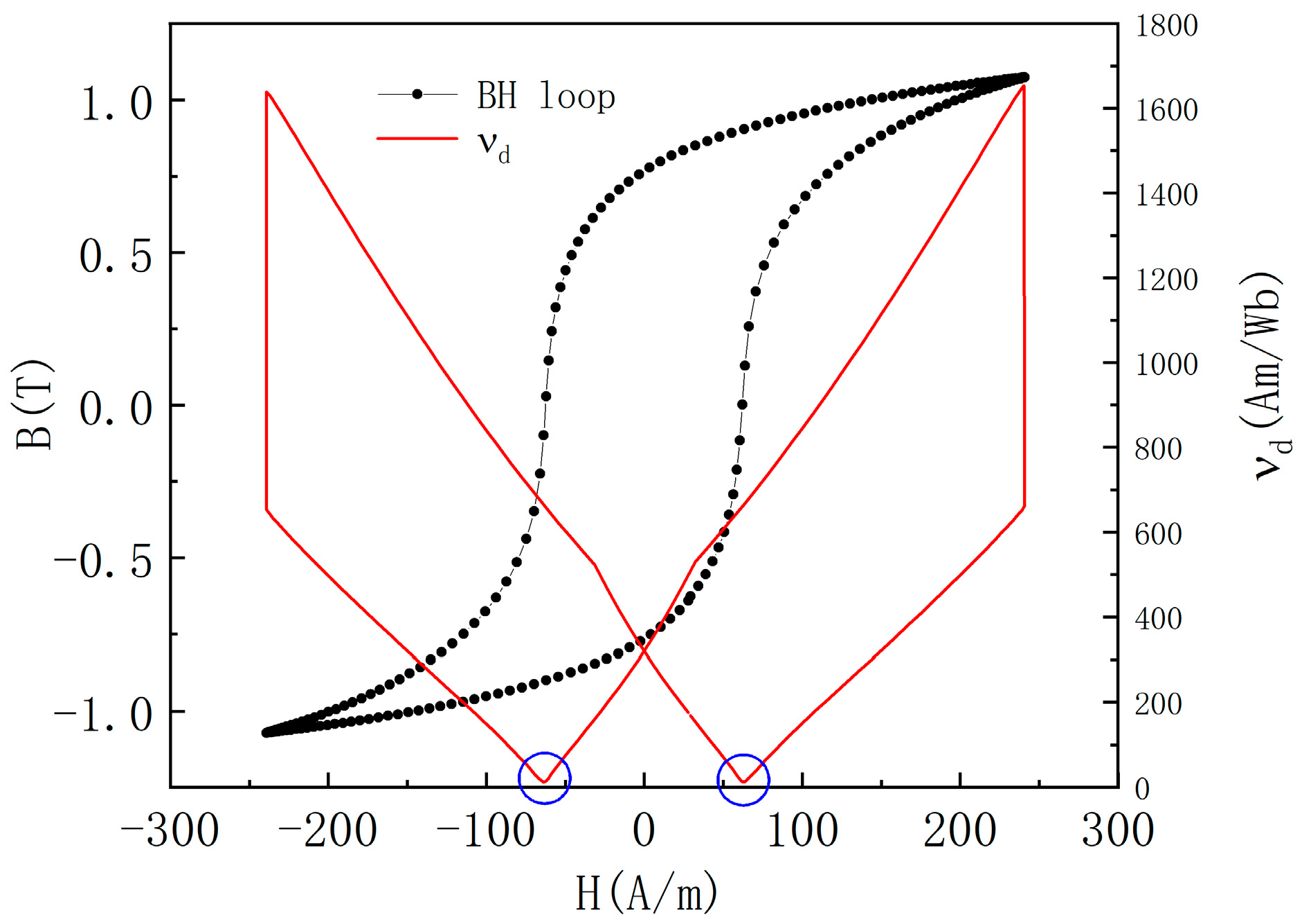
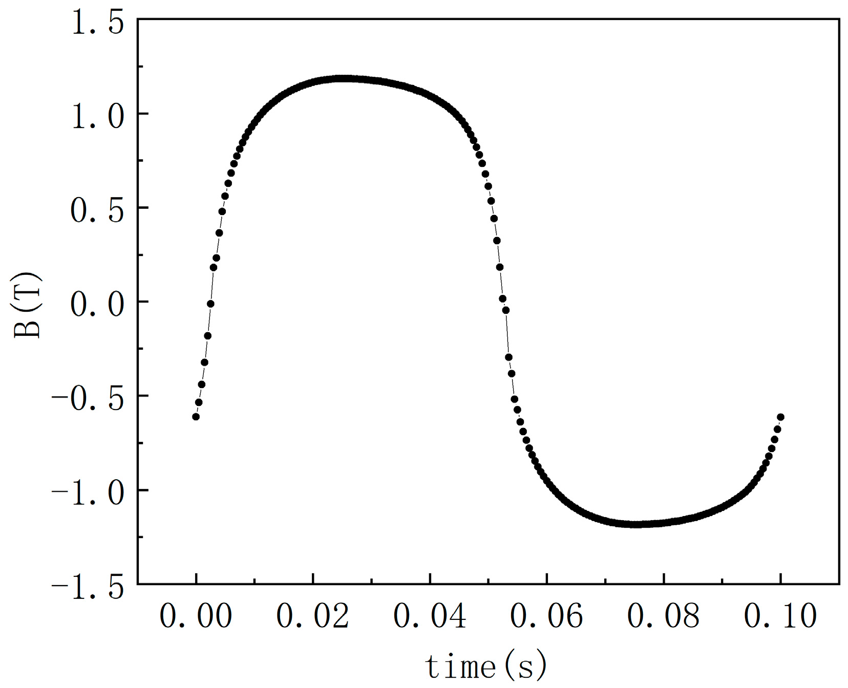
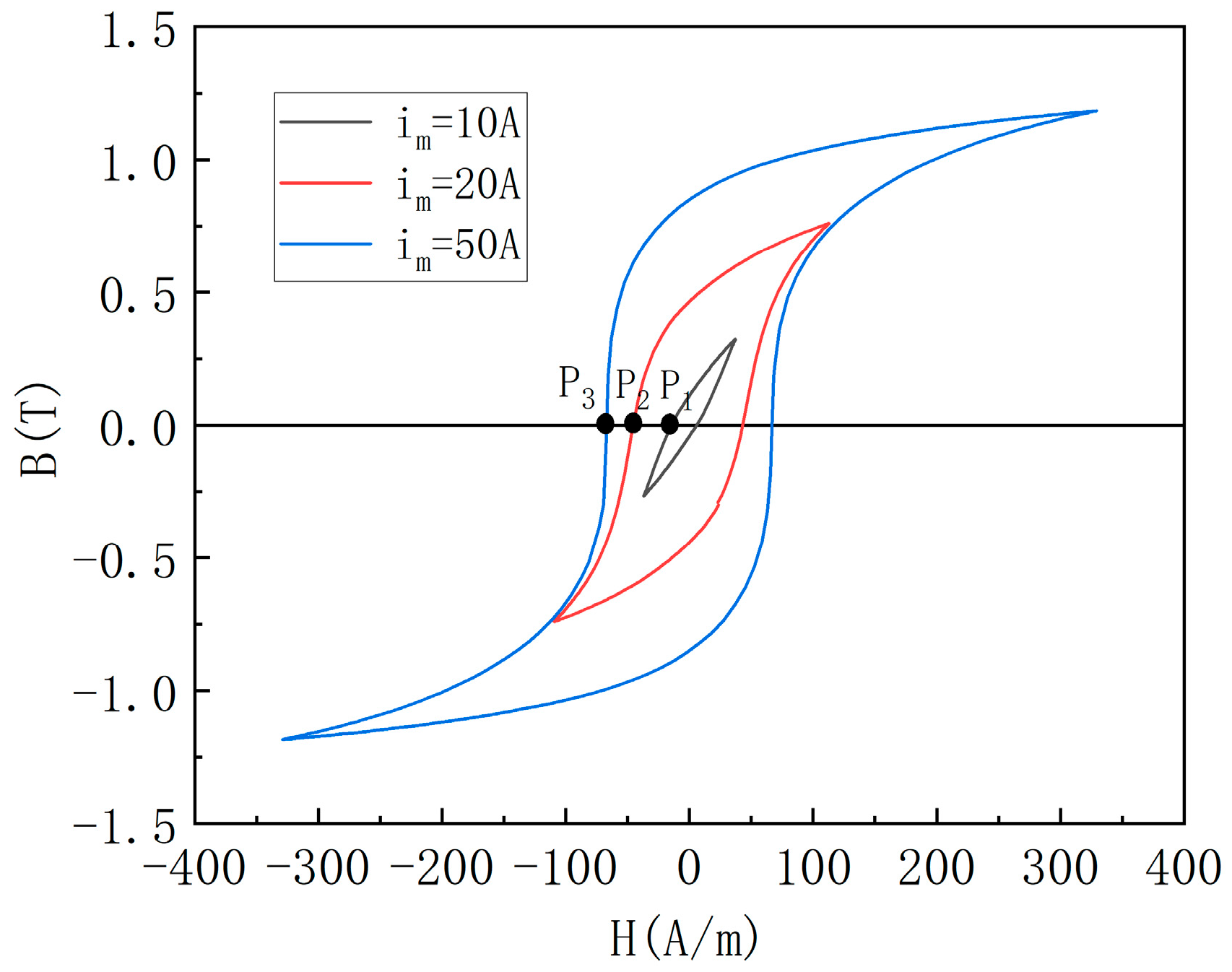
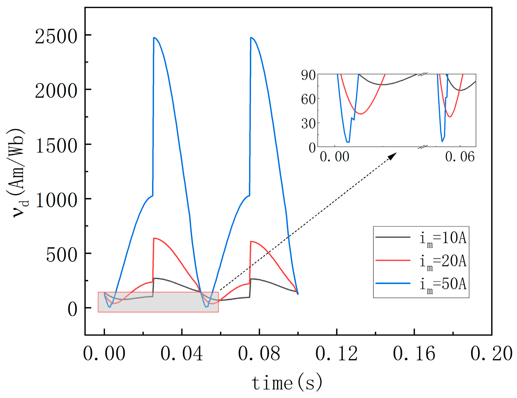
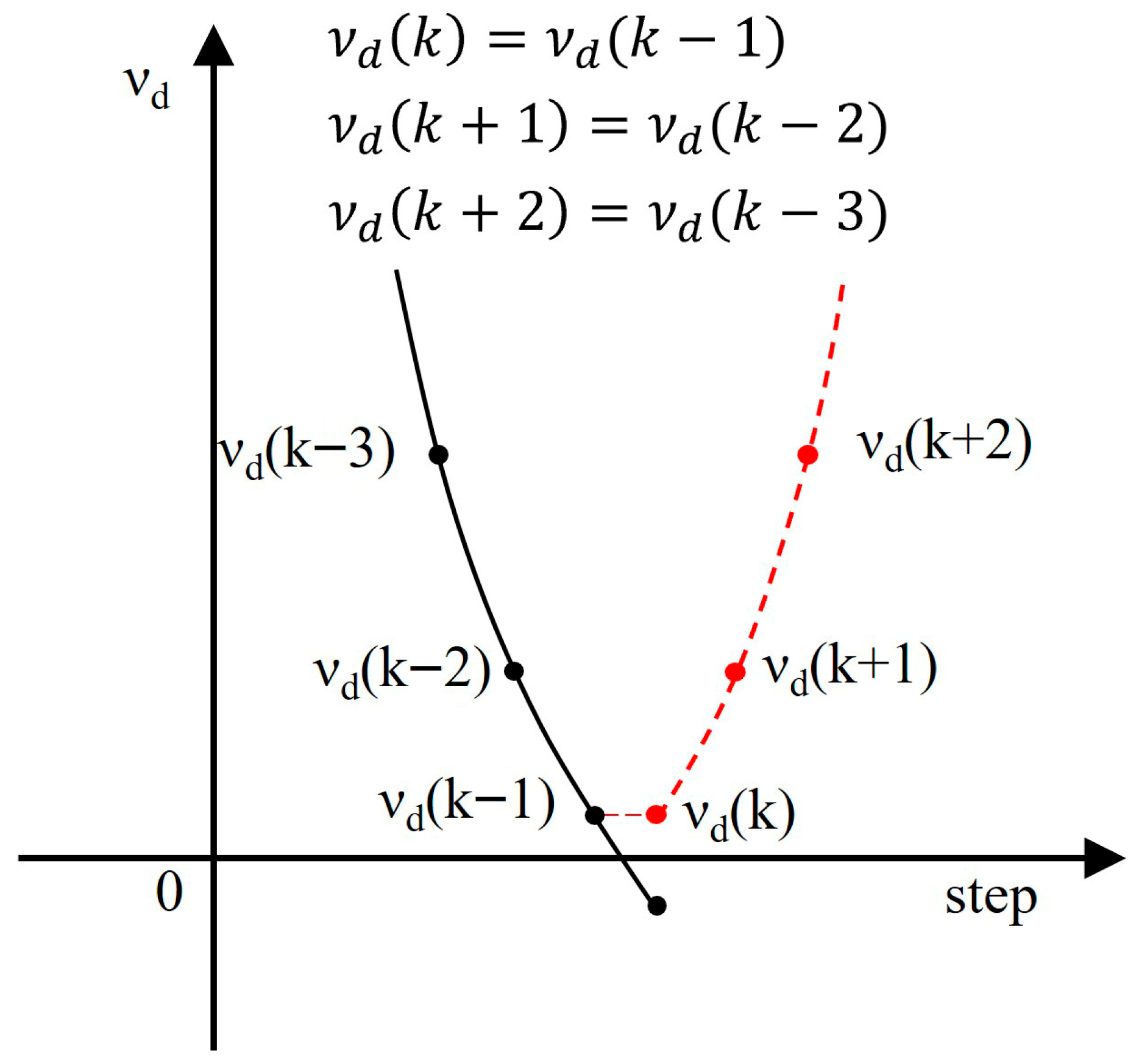
Due to the nonlinear characteristics of ferromagnetic materials, the distribution of data points on the hysteresis loop calculated by the transient finite element method is not uniform within a constant time-step, as shown in Figure 2. The corresponding magnetic flux density waveform is shown in Figure 3. It can be seen from Figure 2 and Figure 3 that the data points are sparse near the zero-crossing points of the magnetic flux density. In this region, B changes quickly, and H changes slowly. The differential permeability reaches its maximum value, while the corresponding differential reluctivity reaches its minimum. At the zero point of B, the greater the excitation is, the more the magnetic reluctivity approaches zero, as shown in Figure 4 and Figure 5, where νd(P3) < νd(P2) < νd(P1). During the simulation, the time-step needs to be sufficiently small at this region to avoid the negative differential reluctivity caused by the numerical error and thus assure the convergence of the iterations. The adaptive time-step can be utilized to stabilize the iterations. However, additional computation overhead is introduced at the same time. This paper proposes a local stability algorithm that can stabilize the iterations without resorting to finer time discretization. It can be observed that the local differential reluctivity νd is asymptotically symmetric relative to its minimum value, as shown in Figure 2, when the magnetic flux density crosses zero. This property can also be observed in the time domain, as shown in Figure 5. The proposed stabilization approach leverages this property. When a negative differential reluctivity is encountered, the minimum value of the differential reluctivity is assumed to have been reached between the current time-step and the previous one. A central point is selected midway between these two steps, and the values of the differential reluctivity for the next several time-steps are set to be equal to their symmetric counterparts relative to this central point. This stabilization continues until the calculated differential reluctivity exceeds the value from the previous step. At this point, the local stabilization algorithm terminates, and the standard FEM calculation flow incorporating the JA model (as illustrated in Figure 1) resumes. Because the proposed differential reluctivity stabilization algorithm is based on the approximate symmetry of the hysteresis loop, any factors that disrupt the symmetry of the hysteresis loop will render the method proposed in this paper no longer applicable, such as under rotating magnetization, DC bias, or harmonic excitation. Only when the alternating magnetization, i.e., the coil excitation, remains in phase, does the method proposed in this paper have good applicability. It should be noted that when the excitation amplitude is small, the maximum magnetic flux density is much lower than the saturation inductance. At this time, near the zero point of the magnetic flux density, the minimum value of the differential reluctivity is usually much higher than zero, which means that it is not easy to cause non-convergence by negative differential reluctivity. Therefore, convergence improvement methods are usually not needed. The schematic diagram of the local stabilization process is shown in Figure 6, and the pseudocode flow chart is shown as follows:
1: bool νd_min = false
2: for (k = 0; k < steps; k++) do
3:  int index_min = 0
4:  int steps_T = T/stepsize
5:  int k_stage = k-steps_T*int(k/steps_T)
6:  if k_stage == steps_T/4 || k_stage == steps_T*0.75
7:     νd_min = false
8:  end if
9:   νd(k) = (H(k) − H(k − 1))/(B(k) − B(k − 1))
10:   if  νd(k) < 0 && νd_min == false
11:    νd(k) = νd(k − 1)
12:      νd_min = true
13:      index_min = k
  Once the calculated differential reluctivity has a negative value, the current value is forcibly assigned to the value of the previous time, and the current value is taken as the lowest differential reluctivity.
14: end if
15: if  νd_min
16:    ifνd(k) < νd(k − 1)
17:       νd(k) = νd (k − index_min − 1)
18:    end if
19: end if
20: end for
Figure 7 shows the effectiveness of the stabilization algorithm. It can be observed that without local treatment, the trajectory of the differential reluctivity shows great numerical oscillation after reaching a locally negative value around zero magnetic flux density (black line in Figure 7). In contrast, with the proposed stabilization method, the differential reluctivity can be effectively stabilized, so that the nonlinear iterations of the JA model coupled with FEM analysis can be converged.

4. Numerical Example

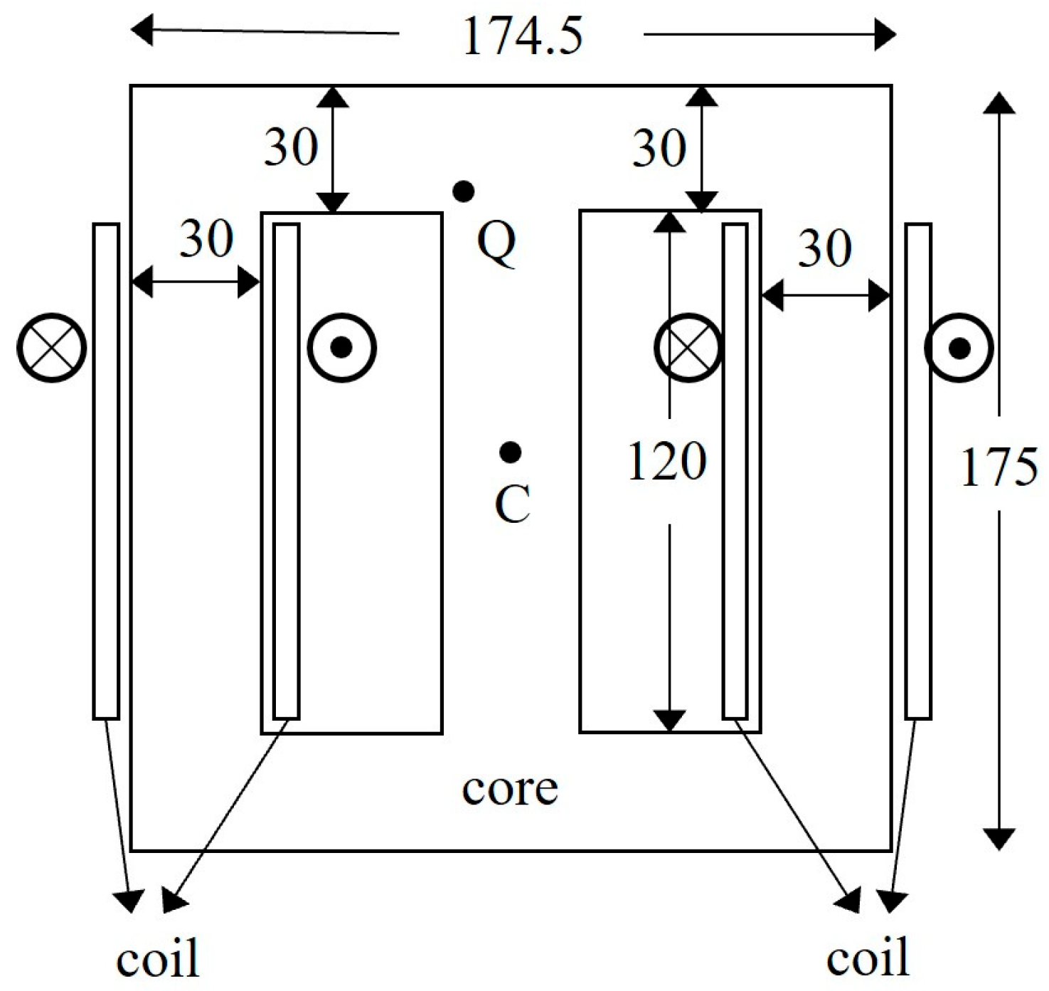
A two-dimensional transformer core model is used to verify the stabilization method proposed in this paper. The geometric model is shown in Figure 8. The two coils are driven by a 10 Hz sinusoidal current with an amplitude of 100 A and the flux generated by the two coils flows in the same direction in the middle column. The 5 JA model parameters of the iron core material are as follows: Ms = 1.33 × 10⁶(A/m); a = 172.86 (A/m); α = 4.17 × 10⁻⁴; k = 232.65 (A/m); and c = 0.652. An air domain with a width of 250 mm and a height of 350 mm is set around the iron core, and the boundary condition of the air domain is that the divergence of the magnetic flux density B is zero.
The finite element calculation incorporating the scalar JA model and vector JA model introduced in Section 2.1 and Section 2.2, respectively, is carried out on an in-house electromagnetic simulation platform, EMPbridge. For the validation of the proposed method, both the scalar and vector JA models are examined by using, respectively, the adaptive time-step method and the proposed stabilization method.
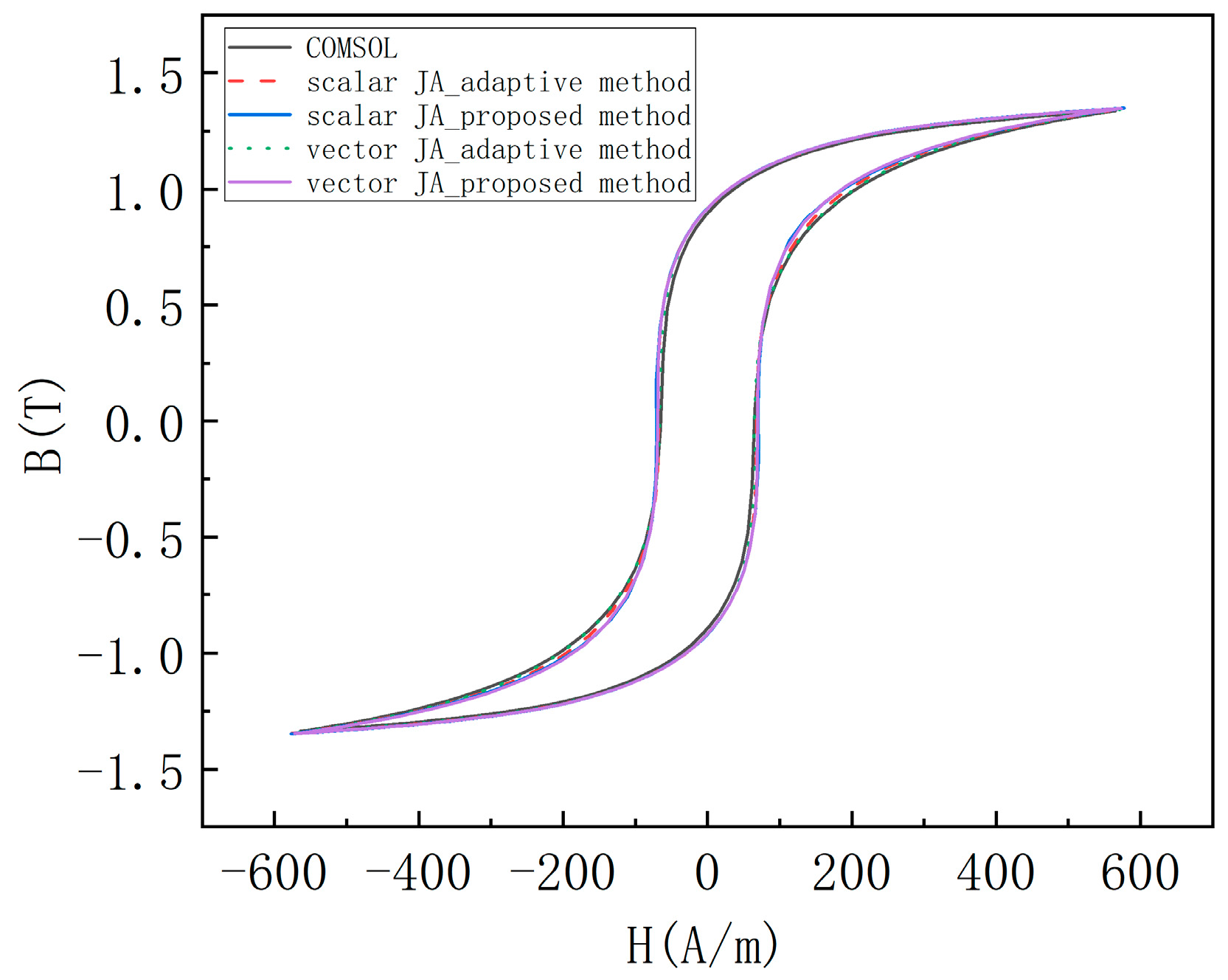
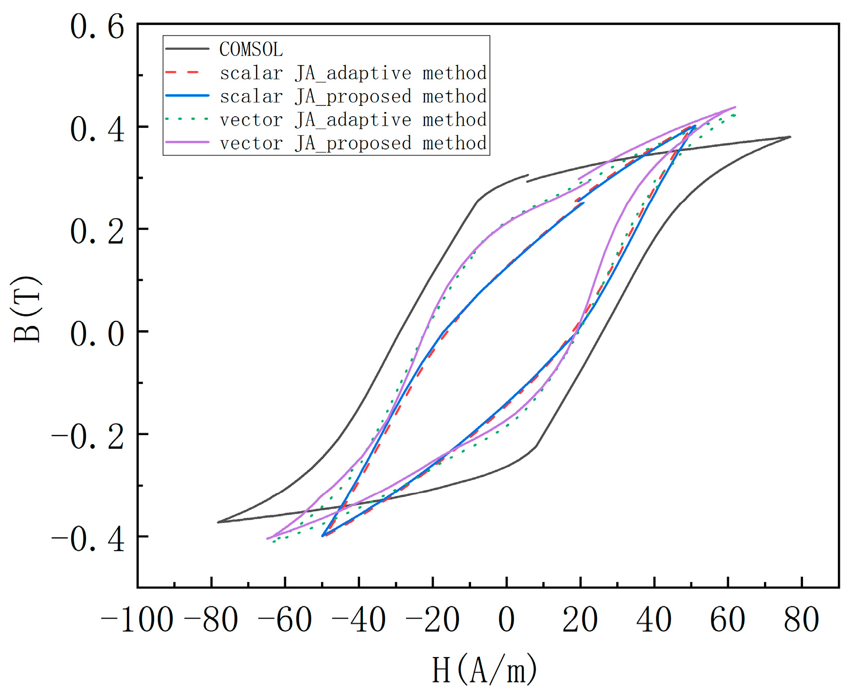
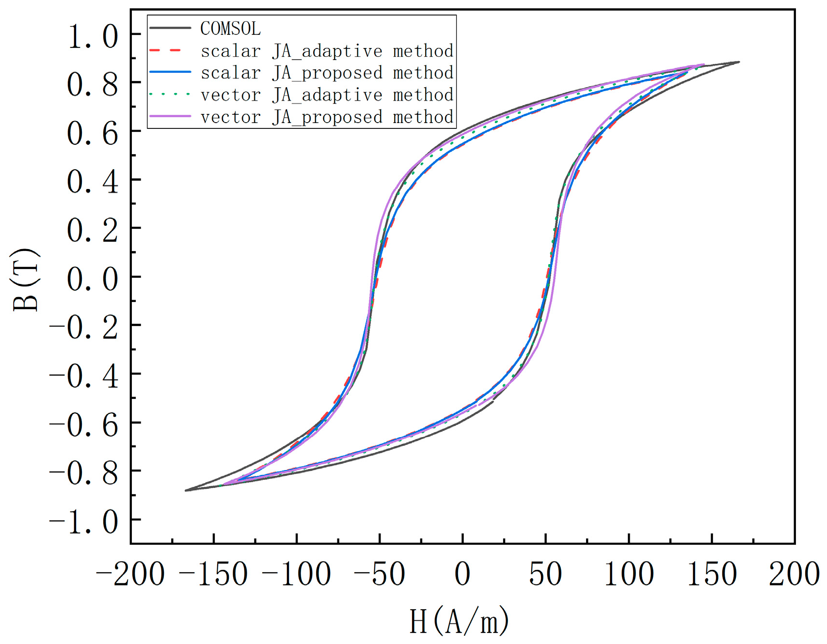
The number of time-steps per period is set as 200, and the simulation is run for two periods. The hysteresis loops at points C and Q, located, respectively, in the center and at the corner of the middle column, as denoted in Figure 8, are simulated. The simulation results, compared with those calculated by the commercial software COMSOL 6.3, are shown in Figure 9, Figure 10 and Figure 11.
Since the magnetic flux density at point C is mainly in the y direction, while the magnetic flux density at point Q has a significant proportion in both the x and y directions, we compared the y component of the hysteresis loop at point C with the x- and y components of the hysteresis loop at point Q.
It can be noticed that the results of both the scalar and vector JA models for the adaptive time-step method and the proposed stabilization method correspond closely to each other at both points C and Q, as shown in Figure 9, Figure 10 and Figure 11. The stabilization algorithm significantly reduces the number of solving steps, as shown in Table 1, and the larger the excitation amplitude is, the more obvious the optimization effect is. It is not easy to directly evaluate the error between different hysteresis loops with different numbers of data points. The error of the hysteresis loop area can be used as an indicator to evaluate the difference between the hysteresis loop results of the proposed stabilization algorithm and the adaptive method, and the hysteresis loop area is proportional to the hysteresis loss, thus also reflecting the error of hysteresis loss. The hysteresis loop area error is shown in Table 2. The error formula is shown in (16). However, the hysteresis loop results of the x component at point Q in Figure 10 show significant differences between the vector and the scalar JA models, which can be explained by the lack of fitting accuracy of the JA models under low magnetic induction in the x direction.
E r r o r = ( S 1 S 2 ) / S 2
Here, S1 and S2 represent the area of the hysteresis loop obtained by the proposed method and the adaptive method, respectively.
Table 1. Comparison of calculation performance of the adaptive time-step method and the proposed stabilization method.
JA ModelMethodNumber of
Time-Steps
Calculation Times (s)
scalar JAadaptive method47373
scalar JAproposed method40045
vector JAadaptive method1789569
vector JAproposed method40069
Table 2. The error of the hysteresis loop area of the adaptive time-step method and the proposed stabilization method.
PointError of Scalar JA ModelError of Vector JA Model
C_y2.1%−6.5%
Q_x0.6%3.7%
Q_y1.4%2.8%
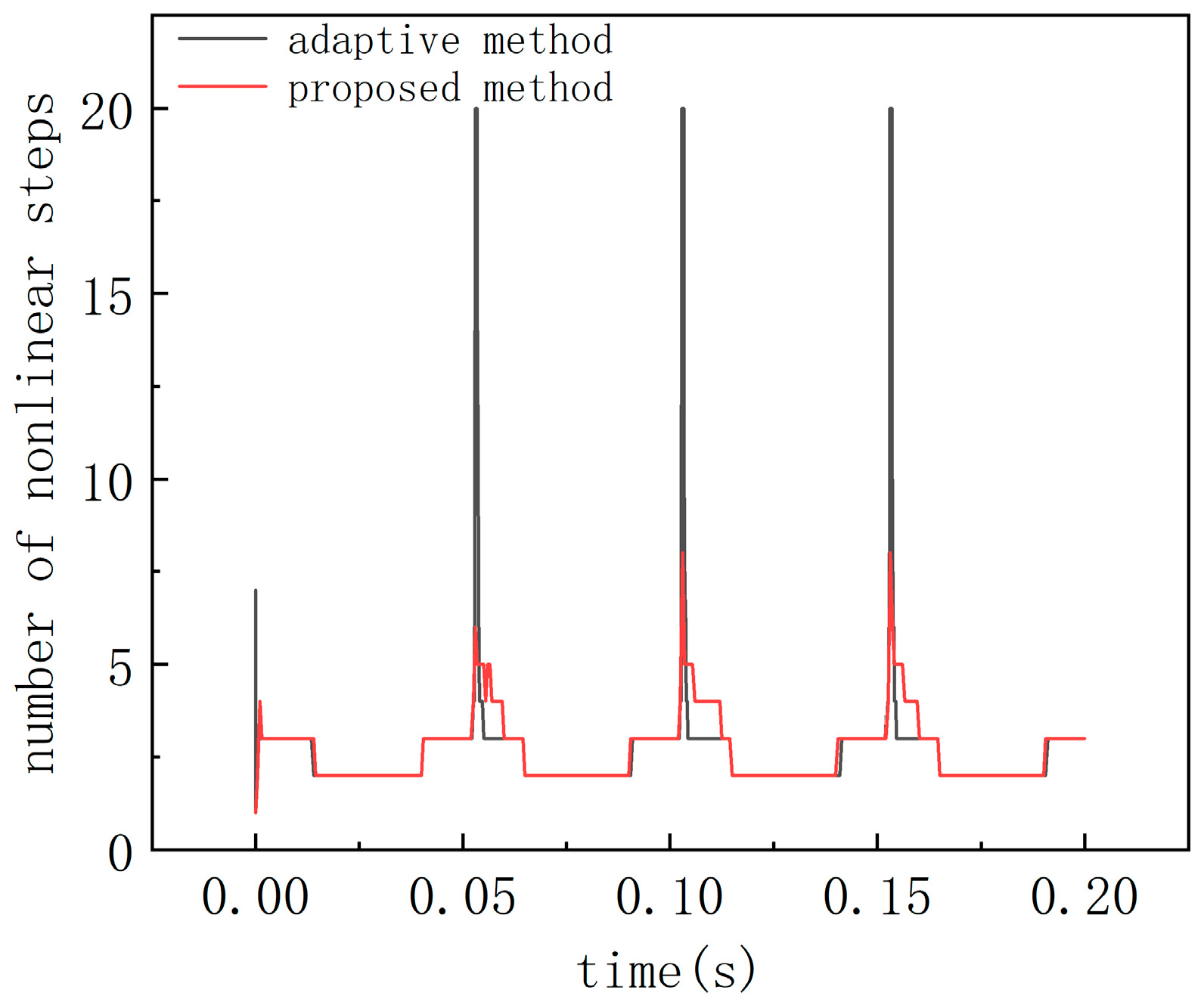
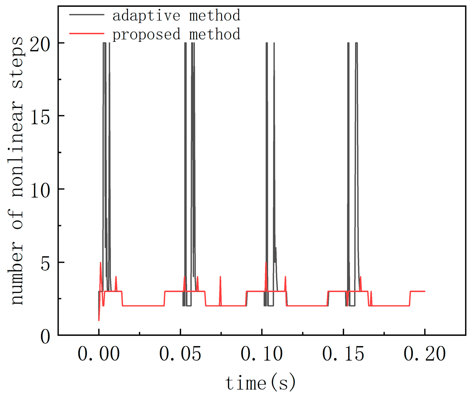
In Table 1, the simulation times of different setups are compared. As expected, when the adaptive time-step is used, extra refined time-steps are taken near the B-field zero-crossing regions, so that the number of time-steps and the computational cost are significantly increased, especially for the vector JA model. In comparison, with the proposed stabilization approach, both the number of time-steps and the nonlinear iteration steps are much lower and stable. The numbers of nonlinear iteration steps over time for the scalar and vector JA models are shown in Figure 12 and Figure 13. It is clearly shown that the adaptive time-step method leads to significant increases in both time-steps and the number of nonlinear iterations. The method proposed in this paper greatly reduces the difference in computational cost between the scalar and vector JA models.
From Table 2, it can be seen that the stabilization algorithms have a smaller impact on the scalar JA model than the vector JA model.

5. Conclusions

In this paper, a localized stabilization strategy based on the local asymptotic symmetry of the hysteresis loop at the zero-crossing region of the magnetic flux density is proposed for regulating the differential reluctivity in instability-prone regions of the hysteresis loop. The proposed method can stabilize the nonlinear iteration while avoiding local refinement of the time resolution, thus reducing the overall computation time. The reliability and efficiency of the proposed method are verified by the simulation of a transformer.

Author Contributions

Conceptualization, X.F.; Writing—original draft, X.F.; Coding, X.F., Y.Z., S.Y. and X.X.; Supervision, S.Y., Y.Z., Z.C., X.X. and Z.R. All authors have read and agreed to the published version of the manuscript.

Funding

This work was supported by the Strategic Priority Research Program of the Chinese Academy of Sciences (XDB0640000) and the National Natural Science Foundation of China (52277019).

Institutional Review Board Statement

Not applicable.

Informed Consent Statement

Not applicable.

Data Availability Statement

The original contributions presented in this study are included in the article. Further inquiries can be directed to the corresponding author.

Conflicts of Interest

The authors declare no conflicts of interest.

References

  1. Leite, J.V.; Benabou, A.; Sadowski, N. Transformer Inrush Currents Taking Into Account Vector Hysteresis. IEEE Trans. Magn. 2010, 46, 3237–3240. [Google Scholar] [CrossRef]
  2. Wang, Y. Research on Residual Magnetism Prediction of Transformer Core. Ph.D. Thesis, Shandong University, Jinan, China, 2017. [Google Scholar]
  3. Jiles, D.; Atherton, D. Theory of ferromagnetic hysteresis. J. Magn. Magn. Mater. 1986, 61, 48–60. [Google Scholar] [CrossRef]
  4. Preisach, F. Über die magnetische Nachwirkung. Z. Phys. 1935, 94, 277–302. [Google Scholar] [CrossRef]
  5. Sadowski, N.; Batistela, N.J.; Bastos, J.P.A.; Lajoie-Mazenc, M. An inverse Jiles-Atherton model to take into account hysteresis in time-stepping finite-element calculations. IEEE Trans. Magn. 2002, 32, 797–800. [Google Scholar] [CrossRef]
  6. Bergqvist, A. A simple vector generalization of the Jiles-Atherton model of hysteresis. IEEE Trans. Magn. 1996, 32, 4213–4215. [Google Scholar] [CrossRef]
  7. Leite, J.V.; Sadowski, N.; Kuo-Peng, P.; Batistela, N.J.; Bastos, J.P.A.; de Espíndola, A.A. Inverse Jiles-Atherton vector hysteresis model. IEEE Trans. Magn. 2004, 40, 1769–1775. [Google Scholar] [CrossRef]
  8. Hoffmann, K.; Bastos, J.P.A.; Leite, J.V.; Sadowski, N.; Barbosa, F. A Vector Jiles–Atherton Model for Improving the FEM Convergence. IEEE Trans. Magn. 2017, 53, 7300304. [Google Scholar] [CrossRef]
  9. Mathekga, A.M.E.; McMahon, R.A.; Knight, A.M. Application of the Fixed Point Method for Solution in Time-stepping Finite Element Analysis Using the Inverse Vector Jiles-Atherton Model. IEEE Trans. Magn. 2011, 47, 3048–3051. [Google Scholar] [CrossRef]
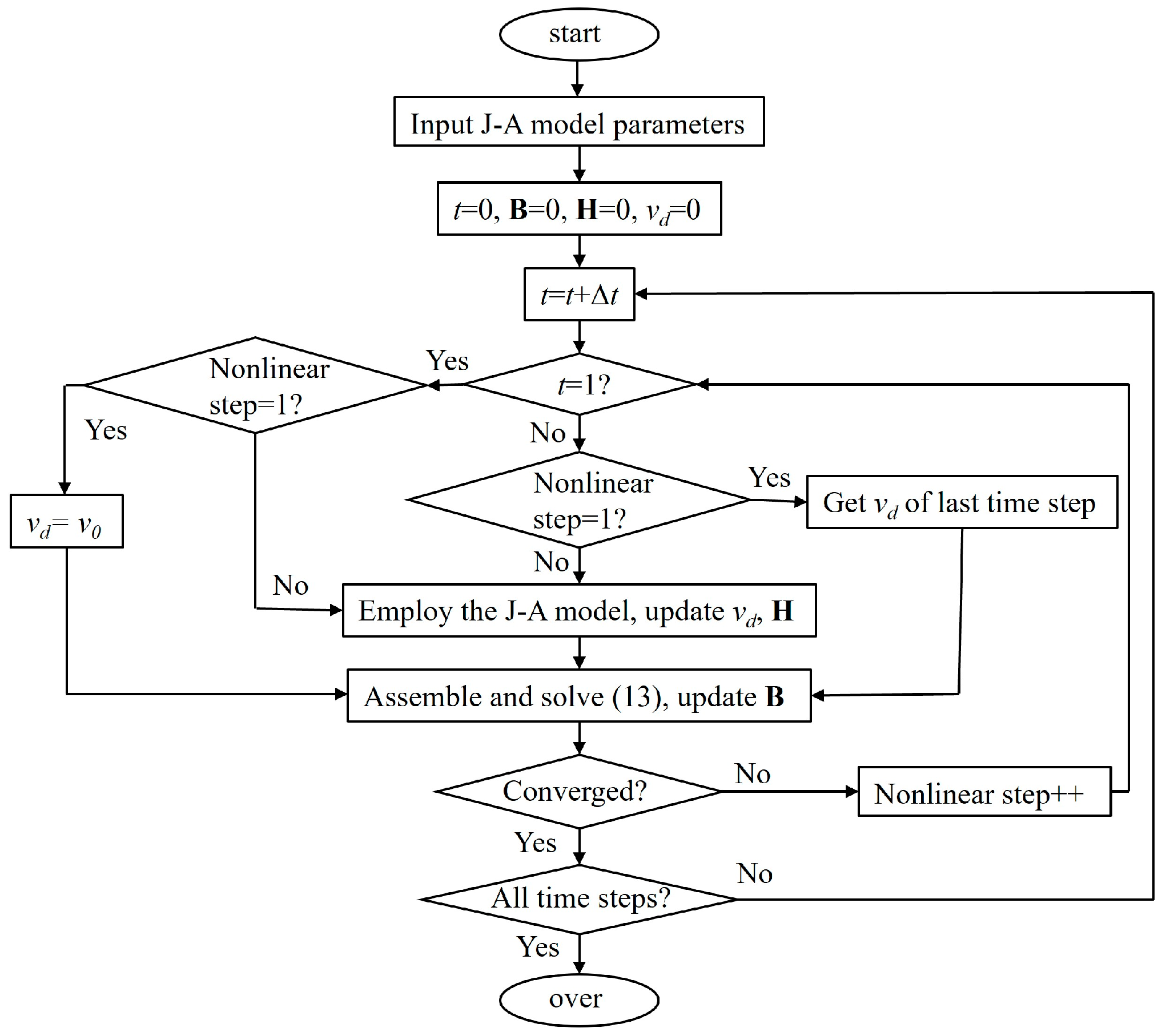
Figure 1. Fitting results of JA model at different magnetic inductions.
Eng 06 00289 g001
Figure 2. Data point distribution on hysteresis loop and the variation in νd with H; the local asymptotic symmetry regions near the zero-crossing of the magnetic flux density are encircled.
Eng 06 00289 g002
Figure 3. Distribution characteristics of data points on hysteresis loop.
Eng 06 00289 g003
Figure 4. Hysteresis loops under different excitation amplitudes.
Eng 06 00289 g004
Figure 5. Variation in differential reluctivity with excitation amplitude.
Eng 06 00289 g005
Figure 6. Schematic diagram of stabilization adjustment at the extreme point of differential reluctivity.
Eng 06 00289 g006
Figure 7. The effectiveness of the proposed stabilization method. Black line: without local stabilization; red line: with the proposed local stabilization.
Eng 06 00289 g007
Figure 8. The geometric model of the numerical example.
Eng 06 00289 g008
Figure 9. Comparison of the hysteresis loop of the y component at point C for different setups and COMSOL (point C (87.25, 87.5); current frequency: 10 Hz; current amplitude: 100 A).
Eng 06 00289 g009
Figure 10. Comparison of the hysteresis loop of the x component at point Q for different setups and COMSOL (point Q (80, 153); current frequency: 10 Hz; current amplitude: 100 A).
Eng 06 00289 g010
Figure 11. Comparison of the hysteresis loop of the y component at point Q for different setups and COMSOL (point Q (80, 153); current frequency: 10 Hz; current amplitude: 100 A).
Eng 06 00289 g011
Figure 12. The number of nonlinear iteration steps over time for scalar JA model.
Eng 06 00289 g012
Figure 13. The number of nonlinear iteration steps over time for vector JA model.
Eng 06 00289 g013
Disclaimer/Publisher’s Note: The statements, opinions and data contained in all publications are solely those of the individual author(s) and contributor(s) and not of MDPI and/or the editor(s). MDPI and/or the editor(s) disclaim responsibility for any injury to people or property resulting from any ideas, methods, instructions or products referred to in the content.