Fundamentals of Climatology for Engineers: Lecture Note

Abstract

The study of climatology serves as a foundation for students who wish to specialize in water resources, hydrology, or environmental engineering. Climatology is the study of long-term average weather patterns. It is a distinct field of study from meteorology and is subdivided into a number of subfields. In order to predict the future hydrologic and hydraulic scenarios, knowledge of climatology is essential. In other words, climatology allows us to determine the likelihood of snowfall and hail, the amount of solar thermal radiation that can reach a specific location, etc. Climatology focuses frequently on how the climate has changed over time and how these changes have affected people and events. The primary objective of this technical note is to acquaint and encourage engineers with the basics of the climate and its processes so that they can understand the climatic impact on water resource systems as beginners.

1. Introduction

Climatology explains the physical processes of climate, including why it changes geographically and how it interacts with the environment and human activity [1]. The phrase comes from the Greek terms “klima” (equivalent to latitude) and “logos” (talk or study). Climate is a dynamic, interrelated system that includes the atmosphere, land, snow, ice, oceans, and living organisms. The air component of the climatic system is often called “average weather”. Climate is the mean and variability of temperature, precipitation, and wind across long time frames (the classical period is 30 years) [1]. External impacts (called “forcings”) transform the climatic system over time [1]. External forcings include volcanic eruptions, solar variations, and human-caused atmospheric changes, and the whole climatic system is solar-powered [1].

Applied climatology examines the relationship between climate and other phenomena, their effects on humans, and the possibility of manipulating the climate to satisfy human requirements. Applied climatology highlights the interconnection of many fields and the usefulness of climate data. New multidisciplinary climatology fields include bioclimatology, agroclimatology, medical climatology, building climatology, and urban climatology [1].

The Intergovernmental Panel on Climate Change (IPCC) has provided projections for future climate change [2]. Numerous natural systems are impacted by regional climate changes, specifically temperature increases, according to their observational scientific evidence. These challenges are faced by the water resource scientists and managers. Understanding the processes driving the changes, the sequences of the changes, and the manifestation of these global changes at different scales may be advantageous for water resource scientists and managers. Since the changes are likely to affect the fundamental drivers of the hydrological cycle, climate change may have a significant impact on water resources and water resource managers [2].

1.1. Scales of Climate

The scales of climate [3] may be given as follows:

• The microclimate is the local climate at a particular point location (e.g., a climate station, for instance a long-term weather or temperature station.
• The topoclimate is the climate of a certain location (e.g., a valley or hill-slope), for example the long-term climate of a river basin. In this context, we recommend [4,5,6] to the readers.
• The mesoclimate is the climate of a region (e.g., southern Oregon).
• The synoptic climate [7] is the climate of a large area (e.g., 1000 km to 10,000 km).
• The global climate is the climate of the planet.

1.2. Climate and Weather

Climatology and meteorology are closely connected, yet have different time scales. Climate is what we expect, while weather is what we encounter [8]. Climate is a probability distribution (PDF) over which the weather oscillates. Climate is determined by the properties of the Earth system and can be thought of as a boundary value problem, whereas weather is highly dependent on the system’s evolution from moment to moment and can be thought of as an initial value problem. The physical processes can be addressed using a numerical solution to a differential equation, for which the boundary value problem and initial value problem are common terms (see this terminology in the context of hydraulics [9,10] for more details).

Weather forecasting is useful or possible for a few days, at most a week. Climate forecasting, on the other hand, is constrained by modeling capability and insufficient observation. This is not a failure of science, but rather of our capacity to comprehend the inherent properties of the climate. Thus, climate simulations are constrained by gaps in our understanding of the hydrologic cycle, which encompasses cloudiness, ocean behavior, and small-scale processes, as well as the inherent unpredictability of various aspects of climate. Beyond several days, a fundamental dynamical property of the atmosphere imposes a significant constraint on weather forecasting [8,11].

Earth’s climate is highly complex, is built on a series of interconnected processes and phenomena, and has multiple feedback mechanisms (see Figure 1). The cryosphere, which includes the ice sheets of Greenland and Antarctica, continental (including tropical) glaciers, snow, sea ice, river and lake ice, permafrost, and seasonally frozen ground, is a critical component of the climate system [12]. The cryosphere is critical to the climate system for a variety of reasons, including its high reflectivity (albedo) for solar radiation, its low thermal conductivity, its high thermal inertia, its ability to influence ocean circulation via freshwater and heat exchange and atmospheric circulation via topographic changes, its large potential for affecting sea level via land ice growth and melt, and its ability to influence greenhouse gases [12].

2. Radiation and Energy Balance in Atmosphere and Earth’s Surface

Almost all of the energy that powers the planet comes from the Sun. To keep a steady global average temperature, all of the solar radiation that enters Earth’s atmosphere must be sent back into space. This is accomplished by the Earth’s energy balance [14].

On average, 49% (168 Watt/m${}^2$) of total incoming solar radiation is absorbed by the Earth’s surface (see Figure 2 and Figure 3). This heat is radiated back into the atmosphere in three ways: as sensible heat, as evapotranspiration (i.e., latent heat), and as thermal infrared radiation. The majority of this radiation is absorbed by the atmosphere, which then radiates in both directions. The radiation lost to space originates in cloud tops and other regions of the atmosphere that are significantly colder than the surface [15]. As a result, a greenhouse effect occurs. During the day, approximately 342 Watt/m${}^2$ of energy reaches the top of the Earth’s atmosphere. Approximately $30\%$ of sunlight reaching the top of the atmosphere is reflected back to space [15]. Approximately two-thirds of this reflectivity is due to clouds and small particles called “aerosols” in the atmosphere. The remaining one-third of sunlight is reflected by light-colored areas of the Earth’s surface, primarily snow, ice, and deserts [15].

On the other hand, the remaining energy is absorbed by the Earth’s surface and atmosphere. This equates to about 240 Watt/m${}^2$. To compensate for the incoming energy, the Earth must, on average, radiate the same amount of energy back into space (i.e., $R_{in}=R_{out}$) [15]. The Earth accomplishes this through the emission of long-wave radiation. Everything on Earth continuously emits long-wave radiation (see Figure 4). To emit 240 Watt/m${}^2$, a surface must be around –19 ${}^{°}$C in temperature. This is significantly colder than the actual conditions at the Earth’s surface (the global mean surface temperature is approximately 14 ${}^{°}$C). Rather than that, the required −19 ${}^{°}$C is found approximately 5 km above the surface. The Earth’s surface is this warm because of the presence of greenhouse gases, which act as a partial cover for the long-wave radiation emitted by the surface. The term “natural greenhouse effect” refers to this blanketing [15].

2.1. Energy Balance

After accounting for all energy inputs and outputs to and from the hydrologic system, the difference represents the rate of change of storage, just as was done for mass balance continuity. Sensible heat is the portion of a substance’s internal energy, e, which is proportional to its temperature, $T^{°}$C; $e=c_{p}T$, where $c_p$ denotes the specific heat at constant pressure. Latent heat transfers occur at phase transitions, as indicated by vertical energy jumps during melting, sublimation, and vaporization [15].

2.2. Heat Transport Process

The heat transfer process occurs in three distinct ways, conduction, convection, and radiation. In conduction, the molecules in higher-temperature zones collide and transfer energy to molecules in lower-temperature zones. It is commonly measured by using Fourier’s equation: $f_h=-k\left(\frac{dT}{dz}\right)$, where k is the heat conductivity. In convection, heat energy is transported via the mass motion of a fluid. Mathematically, $f_h=-\rho cp{K}_h\left(\frac{dT}{dz}\right)$, where $K_h$ is the diffusivity. In radiation, the energy transfers via electro-magnetic waves (which may occur in a vacuum) at rates determined by their surface temperature. The Stefan–Boltzmann equation provides a way to measure radiation $R_e=E\sigma T^4$, where E is the emissivity of the surface, which is equal to one for a blackbody and $0.97$ for water; the Stefan–Boltzmann constant $\sigma =5.67\times 10$${}^{-8}$ W/m${}^2$·K${}^4$; Wien’s wavelength equals $\lambda =0.0029/T$ meters, indicating that the Sun emits shorter wavelengths than the cooler Earth [15].

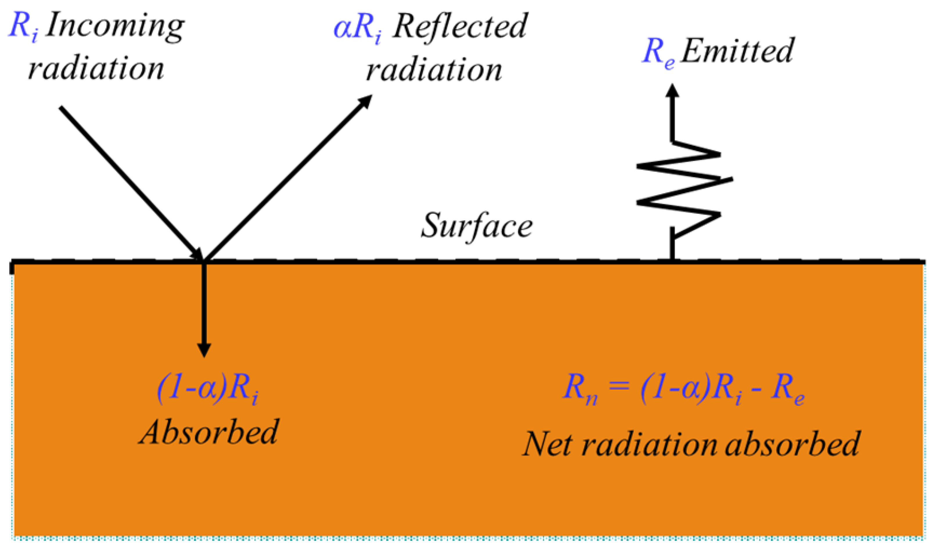
2.3. Radiation Balance at the Surface

The addition of aerosol, dust, and other pollutants to the atmosphere results in the greenhouse effect, in which some of the radiation emitted by the Earth is reflected back by the atmosphere (see Figure 5), resulting in an overall warming of the Earth, an albedo $0\le \alpha \le 1$, i.e., the fraction of radiation reflected, $0.006$ for deep water, and $0.9$ for snow (see [15,18] for details).

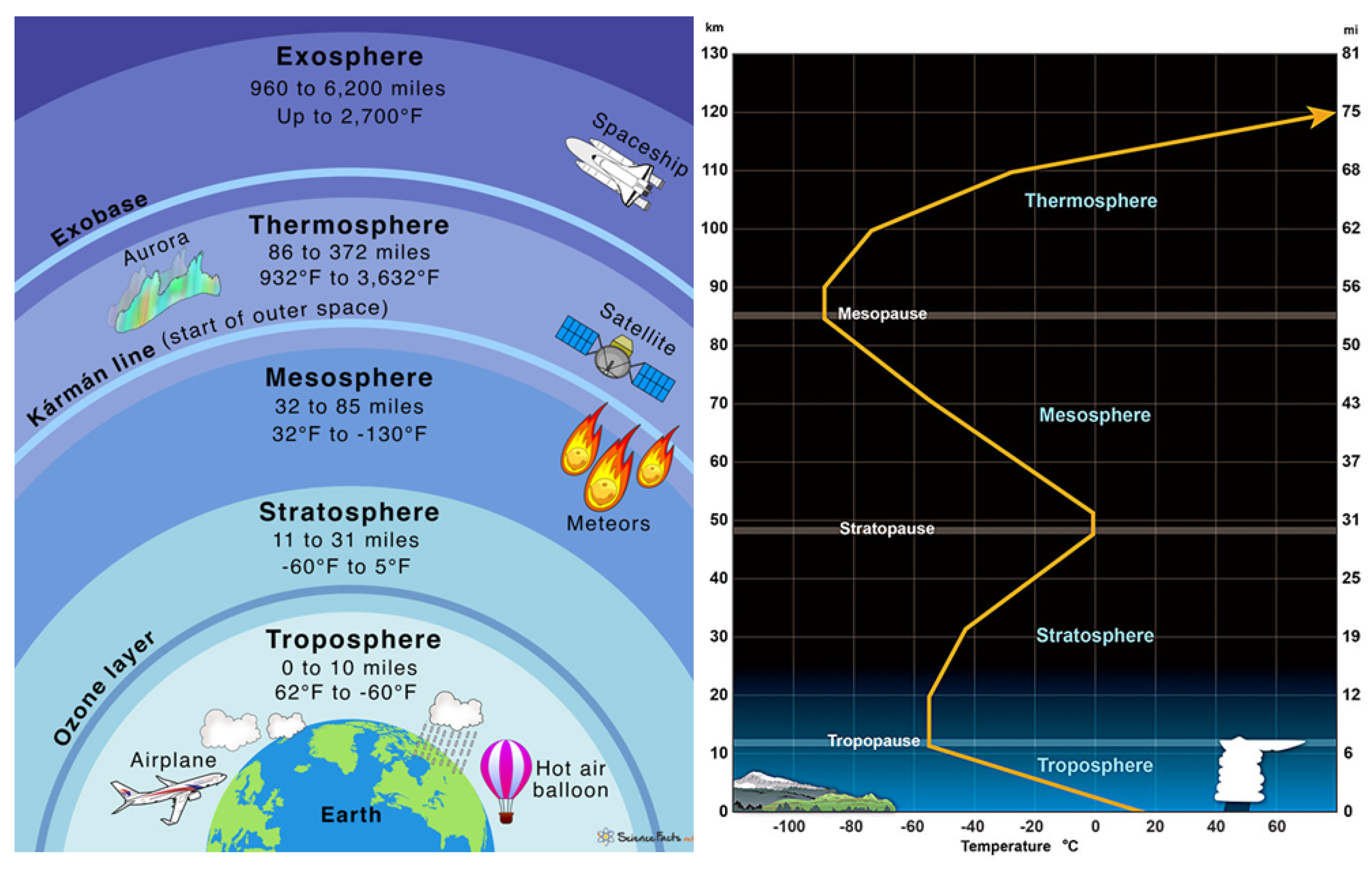
3. Earth’s Atmosphere

The atmosphere is extremely thin in comparison to Earth, reaching a maximum distance of approximately 560 km from the planet’s surface. The structure is divided into four distinct layers (see Figure 6): The troposphere, which extends from 8 to 14.5 km and accounts for approximately $90\%$ of the atmosphere by mass, has a temperature range of about 17 to −52 ${}^{°}$C; at the top of the troposphere, or tropopause (a thin layer), a cold trap causes condensation of the majority of the water vapor, forming clouds below. The dry stratosphere extends up to 50 km in height, with temperatures dropping to −3 ${}^{°}$C due to UV absorption; 99 % of the atmosphere remains below; the stratopause separates the next layer. The mesosphere extends up to 85 km; the temperature drops to −93 ${}^{°}$C; the chemicals are excited due to the Sun’s absorption of energy; the mesopause separates the next layer. The thermosphere reaches a height of 560 km; temperatures can reach 1727 ${}^{°}$C; chemical reactions occur much more rapidly than on the Earth’s surface. Beyond the atmosphere, the exosphere begins at the thermosphere’s top and continues to the interplanetary gases, or space. Hydrogen and helium are the primary components of this region of the atmosphere and are only present at extremely low densities. The greenhouse effect, which keeps us from freezing, is caused by changes in atmospheric temperature with height (see Figure 6) [19].

4. Earth’s Climatic Processes

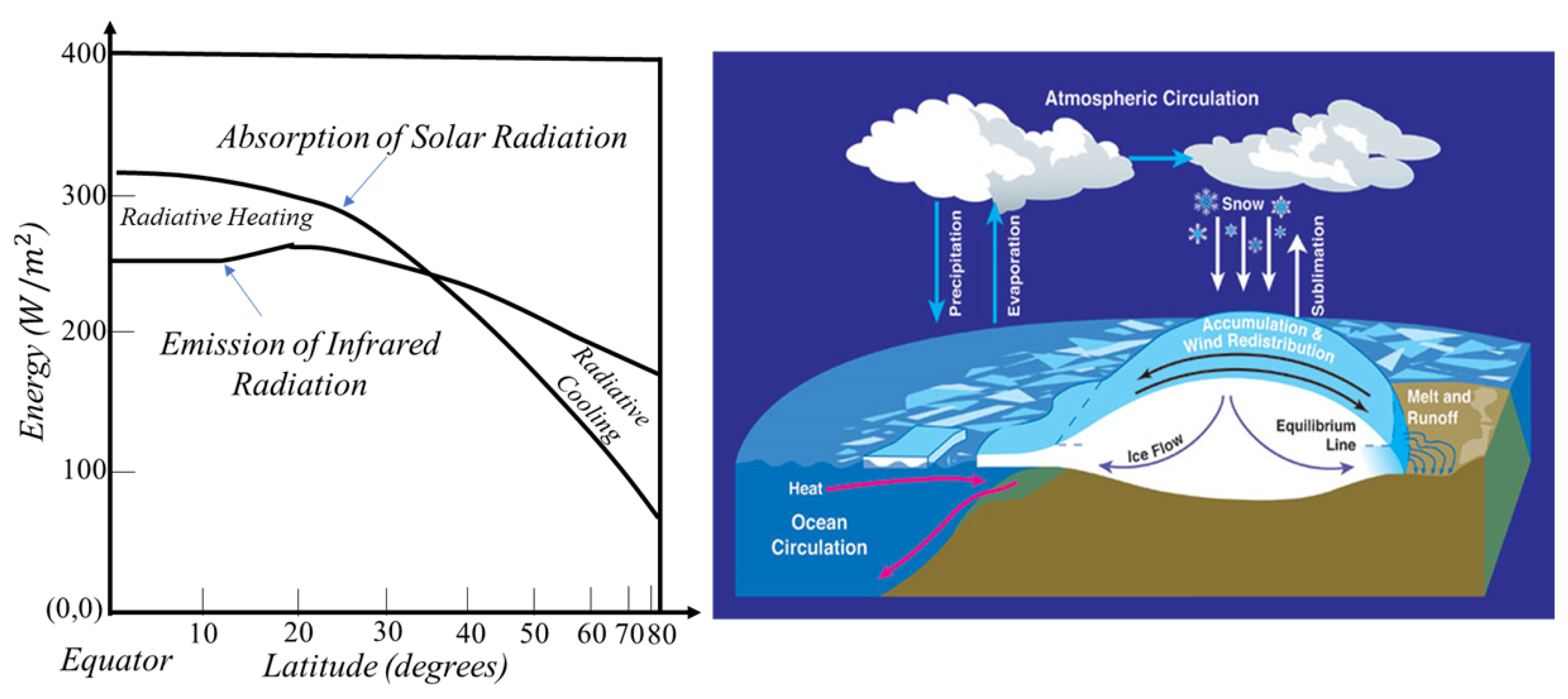
The Earth’s climate is the result of the interaction of various properties and processes: solar radiation and orbital geometry, and the planet’s size, gravitational force, and rotation rate are the most influential, among other things, the composition of the atmosphere, its circulation, and the hydrologic cycle; ocean characteristics and circulation; hydrology, biology, and geochemistry of the land surface; and the geography of continents, glaciers, mountains, and oceans [21].

4.1. Heat Transport

There is a difference between incoming and outgoing radiation, which varies with latitude. Specifically, there is net radiative heating near the Equator and net radiative cooling near the poles (see Figure 7). This imbalance is compensated for by pole-to-Equator energy transport. Thus, a fundamental coupling exists between the Earth’s radiation budget and the general circulation of the oceans and atmosphere. Ocean currents, particularly in the subtropics, transport heat pole-ward in both hemispheres. Heat is transported through the atmosphere in two ways: sensible heat (associated with the air parcel’s temperature) and the latent heat of the water vapor contained within the air parcel; this latent energy (2.5 kJ/gm water) is carried by evaporated water vapor until it is released into the atmosphere via vapor condensation. The atmosphere’s latent heat transport contributes significantly to the Earth’s heat balance; it is a critical link between the hydrologic cycle and the global energy balance [22].

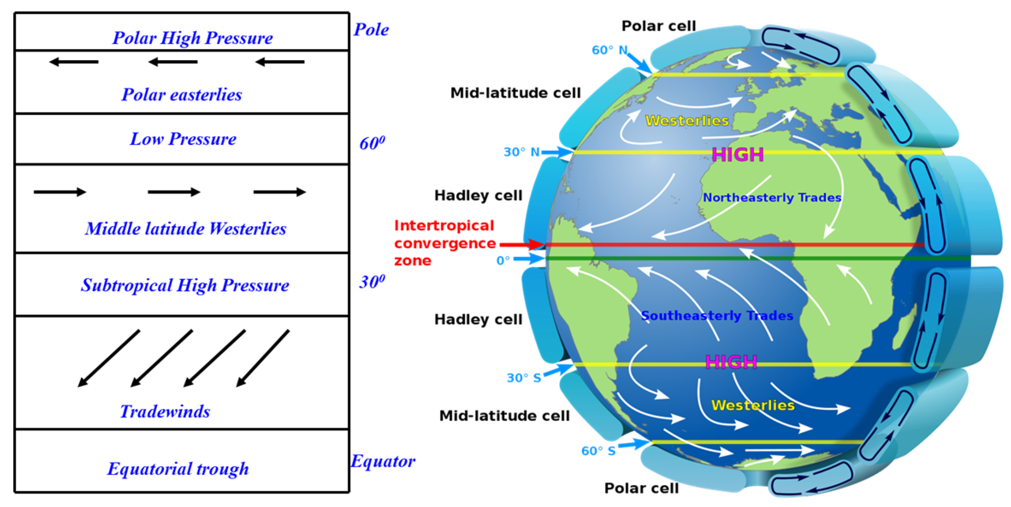
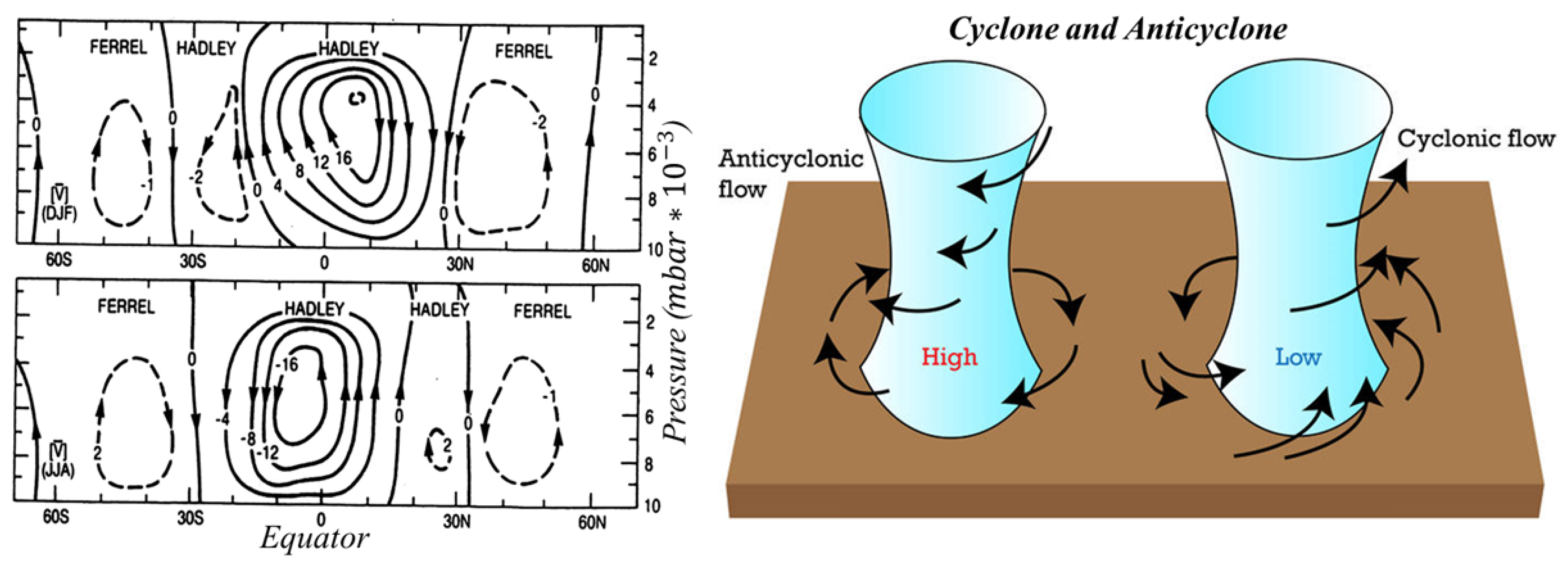
4.2. Atmospheric Circulation

Atmospheric circulation can be broken down into three categories: low-level circulation, upper-level circulation, and general circulation.

4.2.1. Low-Level Circulation

This type of circulation displays significant regional variation in the mean low-level circulation, but a distinct pattern when averaged zonally across a latitude circle. Over the Atlantic and Pacific, the circulation pattern is most prominent. As latitude increases, a low-pressure belt associated with extratropical storm tracks develops, concentrating eastward moving cyclone (low pressure) and anticyclone (high pressure) weather systems. In the Northern Hemisphere, where the contrast between ocean and continent is greater, there are substantial seasonal variations in the atmospheric circulation. In the summer, subtropical oceanic highs expand northward and a region of relatively low pressure develops across South Asia. Wintertime brings storminess to the North Atlantic and North Pacific. Outside of the tropics, the Earth’s rotation is a key factor in determining the circulation–pressure relationship. Flow in a non-rotating system is primarily a direct response to the pressure gradient and is directed away from areas of high pressure and toward areas of low pressure. However, the planet’s rotation produces an additional apparent Coriolis force, resulting in a substantial geostrophic component of flow. This takes the form of a clockwise (CW) circulation around a high-pressure system in the Northern Hemisphere and a counterclockwise (CCW) circulation around a low-pressure system in the Southern Hemisphere (see details in [24]).

4.2.2. Upper-Level Circulation

Due to the thermal and wind’s combined effect, the atmospheric circulation generally intensifies and simplifies as it ascends through the troposphere. Pressure decreases with height more rapidly in colder air than it does in subtropical air, which results in a vertical pressure gradient along the north–south axis with height. Due to the geostrophic relationship between pressure and circulation with altitude, in the subtropics and middle latitudes, strong westerlies develop with altitude. The jet stream is the rise of the strongest westerlies in the upper troposphere. Jet streams are constantly evolving, meandering, and decaying as part of the upper troposphere’s wavy planetary-scale circulation systems. Upper tropospheric circulation characteristics are associated with the extratropics’ ever-changing regional weather regimes (see the details in [24]).

4.2.3. General Circulation

This was considered for the first time in 1735 by George Hadley. Hadley reasoned that the equatorward direction of low-level easterly winds in the vast oceanic trade-wind belts of the subtropics reflects the lower branch of a hemisphere-wide thermal convection cell, with rising motion in the warm equatorial belt and sinking motion in the subtropics and colder-temperature zones. The difference in solar heating between the tropics (23${}^{°}{27}^{\prime }$ N and S) and high latitudes would drive such a circulation. Hadley regarded transient circulations associated with day-to-day weather variation, as well as mean differences in the circulation around a latitude band and the annual cycle of temperature and other metrological elements, as irrelevant “ornaments of the circulation” that are uncoupled from the fundamental processes of the general circulation. Even though mean low-level circulation varies significantly across regions, when data are averaged around a latitude circle, a distinct pattern (mean meridional) emerges (see Figure 8) (see the details in [25]).

The air entering from lower latitudes is generally warmer and will rise in order to cool. As some of this air sinks near the subtropics and returns to the Equator, it produces what are known as trade winds, which were named after sailing ships used in foreign trade between Europe and the New World. The region near the Equator where these winds cease to exist is referred to as the doldrums. Hadley cells are areas where air rises at the Equator, sinks at 30${}^{°}$ north and south, and then flows back to the Equator. Although the trade winds are most distinct over the Atlantic and Pacific, they are frequently influenced by monsoon circulation over the Indian Ocean–Indonesian sector. While the majority of air sinks at 30${}^{°}$ north and returns to the Equator at 30${}^{°}$ south, some air continues to move poleward. The belt of subtropical high pressure is located between 30${}^{°}$ north and south latitudes; as one moves higher in latitude, a low-pressure belt associated with the extratropical storm track (between 40${}^{°}$ and 60${}^{°}$) is formed, concentrating eastward-migrating cyclonic (low pressure) and anticyclonic (high pressure) weather systems. Ferrel cells are circulation cells that form between 30${}^{°}$ and 60${}^{°}$ north and south. At approximately 60${}^{°}$ north and south, the air collides with cold polar air to form polar fronts; some of the air that rises at the polar fronts continues to move poleward, sinking at the poles and then returning to 60${}^{°}$ north and south. There is a tendency for elevated pressure to build up over the cold polar cap. Hadley cells (see Figure 8) are more robust than cells at higher latitudes. The Hadley circulation cannot be adequately described by an annual average; with the exception of brief periods during the equinox seasons (spring and autumn), the tropics’ mean meridional circulation is dominated by a single summer hemisphere Hadley cell. The rising air zone moves seasonally, being in the SH from December to February (southern summer) and in the NH from June to August (northern summer). Outside of the tropics, the components of the mean meridional circulation are quite weak; they are comprised of weak indirect Ferrel cells and even weaker direct polar cells. Outside of the deep tropics, the Earth’s rotation dictates the relationship between circulation and pressure; in a non-rotating system, flow is largely a direct response to pressure gradients (high to low). Because the air that sinks at certain locations flows back along the Earth’s surface in a non-linear north–south path due to the Coriolis effect, this results in a strong geostrophic component of flow. This manifests as a CW circulation around high-pressure (anticyclonic) systems and a CCW circulation around low-pressure (cyclonic) systems in New Hampshire. In SH, the inverse relationship exists. Due to the thermal and wind’s combined effect, atmospheric circulation generally intensifies and simplifies upward through the troposphere; there is an increasing N–S horizontal pressure gradient (pressure decreases more rapidly with height in the north than in the south) with height. Stronger westerlies develop with height in the subtropics and middle latitudes due to the geostrophic component; this axis of the strongest westerlies in the upper troposphere is called the jet stream (speed: 160 km/h). These upper tropospheric circulation characteristics are associated with the extratropics’ ever-changing regional weather regimes; these synoptic characteristics are implied by the relatively low consistency of the wind direction in mid-latitudes (see the details in [25]).

The mean meridional (latitude averaged) circulation of the atmosphere between December and February and between June and August is shown in Figure 9; the values on the streamlines indicate the total mass circulation (1010 kg/s) between that streamline and zero streamline (see the details in [25]).

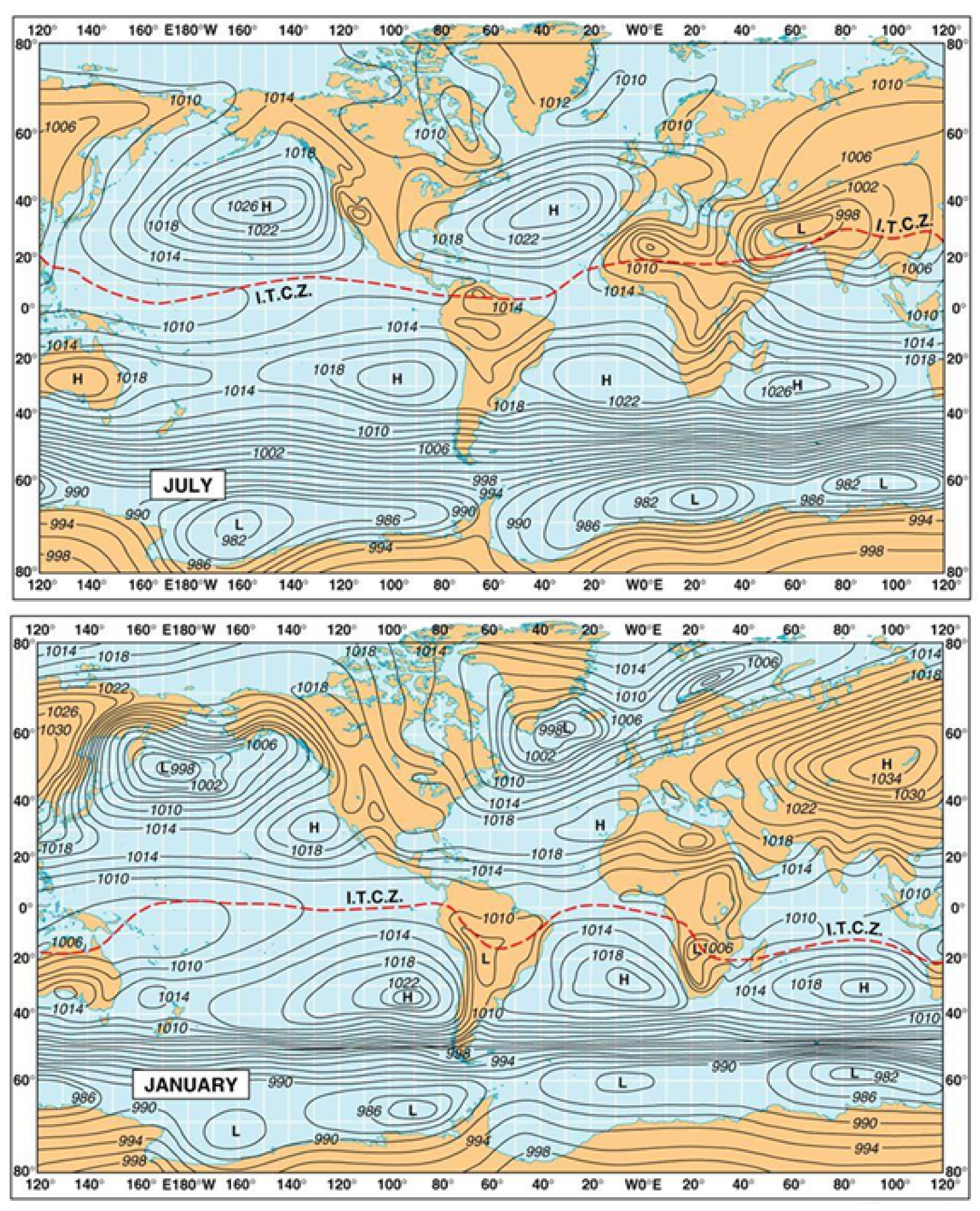
4.3. Global Pressure, Surface Wind Speed, and Sea Surface Temperature (SST)

During northern summer, oceanic subtropical highs develop rapidly and expand northward; relatively low pressure develops over warm continents, most notably South Asia, where the monsoon low is well developed. During northern winter, a seasonal reversal of pressure between continents and oceans is observed; storminess increases over the North Atlantic and North Pacific as a result of pronounced low-pressure areas in northern latitudes and weak high-pressure areas in the subtropics (see Figure 10) (see the details in [26,27,28,29,30]).

Seventy-one percent of the Earth’s surface is covered by ocean water. Due to the fact that water has a greater heat capacity than land, the ocean serves as the primary heat storage or memory component of the climate system. Annual mean SST varies between 29 ${}^{°}$C in portions of the tropics to −1.8 ${}^{°}$C near the ice edge (see the details in [26,27,28,29,30]).

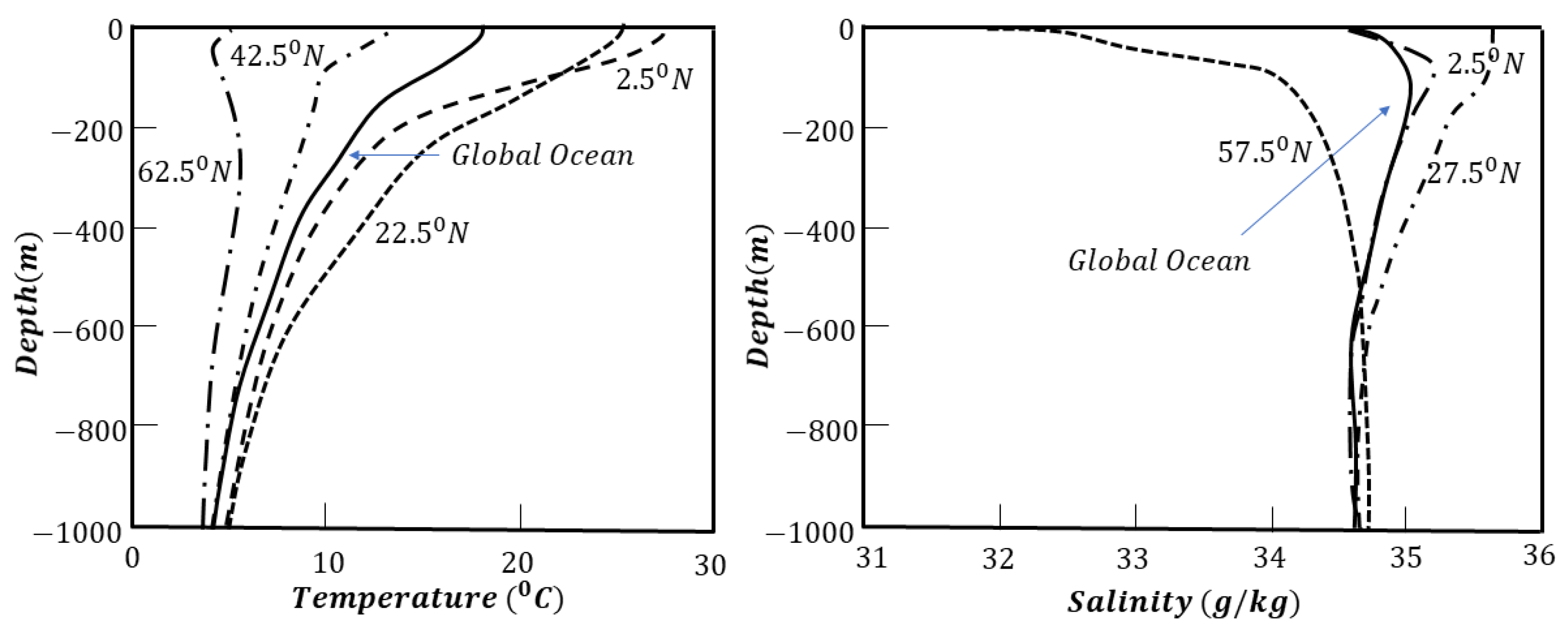
4.4. Ocean Temperature and Salinity Profile

Because the ocean is heated and cooled predominantly from its upper surface, it has a thermal structure distinct from the atmosphere. Oceans are separated into upper and deep zones based on their temperature. Within the upper zone, a mixed layer exists where the temperature is similar to that of the surface. Below the mixed layer lies a transition layer called the thermocline, in which the temperature rapidly lowers. Temperature falls extremely slowly in the deep ocean. At mid-latitudes, a seasonal thermocline forms (see Figure 11) (see the details in [26,27,28,29,30]).

SST isotherms run broadly east–west across the majority of the ocean, but diverge towards the coasts and around the Equator, where currents and upwellings influence the temperature distribution. The ocean and atmospheric circulation systems are linked by energy and momentum exchanges at the air–sea interface. At its lower limit, the atmosphere absorbs energy via conduction against a warmer sea surface, whereas surface wind generates wind-driven circulations in the upper ocean. The ocean responds to surface heat fluxes and evaporation and precipitation, which alter the ocean’s temperature and salinity, resulting in density variations that drive the ocean’s deep thermohaline circulations (see Figure 12) (see the details in [26,27,28,29,30]).

4.5. Wind-Driven Circulation and Ocean Currents

Wind-driven circulation is predominantly horizontal and is confined to the ocean’s upper few hundred meters. The Antarctic circumpolar current is continuous around the latitude circle at the southerly latitudes of the SH, where there are strong and persistent westerlies and no land barrier. Outside the deep tropics, the Atlantic and Pacific Oceans’ largest-scale wind-driven circulation systems are the basin-scale subtropical anticyclonic gyres, which form as a result of prevailing winds, continental boundaries, and the Earth’s rotation. They include the following: warm poleward current systems on the west side of ocean basins that are quite narrow and intense (transport heat): the Gulf Stream in the North Atlantic, the Kuroshio Current east of Japan; currents on the east side of ocean basins that are cold and upwelling (carry cooler water): the California Current in the North Pacific, the Peru Current in the South Pacific. The Equator’s primarily east–west or zonal circulation regimes are significantly different from those seen at higher latitudes; large shifts in these equatorial currents are quick and more in tune with year-to-year atmospheric variability, known as the El Niño–Southern Oscillation (ENSO) (see the details in [26,27,28,29,30]).

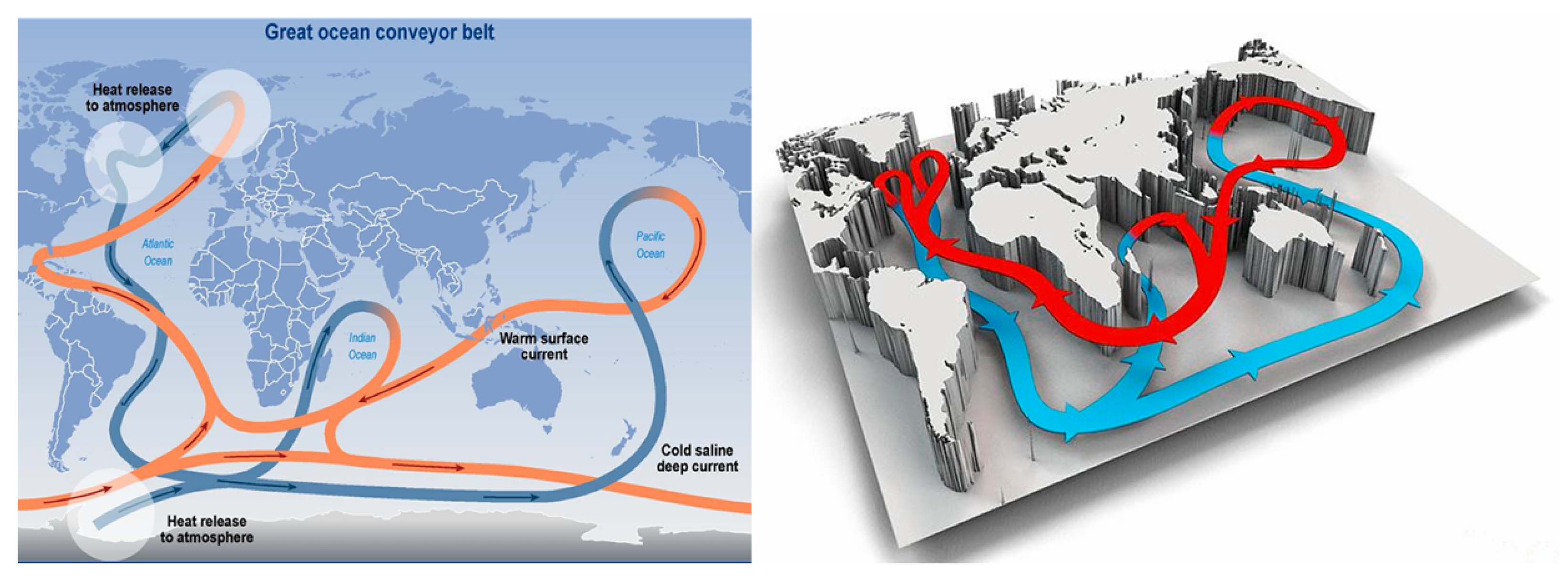
4.6. Thermohaline Circulation

Thermohaline circulation is the slow movement of water through oceans caused by density changes caused by temperature and salinity variations. It begins in polar latitudes as a vertical flow that sinks to the mid-depths or even lower, followed by horizontal flow. It is initiated by an increase in density at the upper surface, either directly through cooling and/or salinity increases or indirectly through ice melting and ejecting salt, thereby increasing the salinity of the remaining water. The global-scale redistribution of ocean water by thermohaline circulations occurs on time scales ranging from decades to centuries, with a typical cycle lasting approximately 1600 years, i.e., water from the surface to the deep ocean and back to the surface (see the details in [26,27,28,29,30]).

The great world ocean’s water is constantly in motion. There are currents that transport enormous amounts of water around the world known as the Great Ocean Conveyor belt [34]. Oceanic thermohaline circulation is what powers the Conveyor. It involves both heat, hence thermo, and salt, hence haline, for common table salt (halite). Temperature and salinity both affect the density of seawater, and the density differences between water masses cause the water to flow. Thermohaline circulation, also known as the Great Ocean Conveyor, results in the world’s largest oceanic current. It operates similarly to a conveyor belt, thus the name, transporting massive amounts of cold, salty water from the North Atlantic to the Northern Pacific and returning with warmer, fresher water. Typically, descriptions of the Conveyor’s operation begin with what occurs in the North Atlantic, beneath and near the polar region’s sea ice. There, warm, salty water transported from tropical regions is rapidly cooled, resulting in vast quantities of frigid water. When this seawater freezes, the salt content of the water is removed (sea ice contains almost no salt), increasing the salinity of the remaining, unfrozen water. The salinity of the water makes it quite dense, and its frigidity makes it even denser. Due to the fact that this water is denser than the less saline, warmer surface waters moving in from the south, it sinks to the ocean floor. Oceanographers refer to this water as North Atlantic Deep Water (NADW), and it is responsible for today’s oceanic thermohaline circulation. This water begins its great circuit through the world’s oceans in the northernmost reaches of the North Atlantic. It travels south through the North Atlantic, then south through the South Atlantic, rounding Brazil, where it meets vast masses of similarly frigid and saline water flowing from beneath the sea ice surrounding Antarctica (dubbed Antarctic Bottom Water (AABW) or Antarctic Deep Water (AADW)), hugging the ocean bottom as it flows. This greatest of ocean currents then moves east, well north of the Antarctic mainland, but well south of Africa (where a branch pushes northward along the east African coast past the Cape of Good Hope) and continues east across the entire width of the Indian Ocean north of Antarctica, swinging around south of Australia and far into the Pacific. As it continues its submarine migration, the current mixes with warmer water, warms, and rises, until it finally dissipates as a coherent entity in the northern Pacific. However, in the Pacific, a warm, shallow-sea counter-current has formed. This counter-current travels south and west through the Indonesian archipelago, across the Indian Ocean, continuing westward, and circles southern Africa just off the Cape of Good Hope. It passes through the South Atlantic, still on the surface (though it extends a km and a half below the surface), where tropical warmth increases evaporation, making the counter-current saltier. It then travels up the East Coast of North America and across the Atlantic to the coast of Scandinavia, where its warmth helps protect residents from the bitter cold of northern winters. When this saltier, warmer water reaches high northern latitudes, it cools and eventually transforms into North Atlantic Deep Water, completing the circuit (see the details in [26,27,28,29,30]).

5. Coupled Ocean and Atmosphere Processes

5.1. Annual Cycle and Monsoon Circulation

The annual climate cycle amplitude is significantly greater in the NH (60% ocean) than in the SH (80% ocean), because the seasonal cycle of land surface temperatures is moderated by ocean heat storage during the summer and release during the winter (via poleward transport). During the winter, high-latitude continents propel cold air masses southward and eastward from Asia and North America, bringing them to the warm waters of the western Pacific and Atlantic via transient cyclones and associated cold fronts. The heat fluxes from the oceans modify cold continental air masses as they travel eastward across the oceans, with the air assuming maritime characteristics well before it reaches the west coast of North America or Europe. While maritime influence extends far inland in Europe (there are no mountain barriers), it is largely confined to the area west of major coastal mountain barriers in North America (see the details in [26,27,28,29,30]).

The annual cycle of land surface temperature has a greater amplitude than the tropical sea surface temperature cycle (SST). The annual cycle of land–ocean surface temperature difference, combined with the seasonal reversal of the SST difference between the hemispheres, is what drives the tropics’ atmospheric monsoon circulations (see the details in [26,27,28,29,30]).

The Asian–Australian monsoon system is the world’s dominant monsoon circulation. During the winter, there is a low-level flow of dry and cool air from the cold continent to the warm ocean, resulting in a light precipitation over land. During the summer, moisture flows from the tropical ocean to the warmer land, where the upward motion of the heated air produces monsoon rains. The monsoon component of atmospheric surface circulation indicates the monthly mean surface circulation’s departure from its annual mean value. Similar but less-pronounced monsoon-type circulations also occur over western Africa, parts of Mexico, and Central America, extending as far north as the southwestern United States. Additionally, the 28 ${}^{°}$C and 27 ${}^{°}$C SST isotherms for the respective hemisphere’s mid-summer month are shown; hatched areas indicate significantly higher precipitation than the average for all months. Apart from these shared characteristics, regional monsoon precipitation regimes vary significantly (see the details in [26,27,28,29,30]).

5.2. Tropical Cyclones

Each of the short-lived depressions and storms in the tropics is composed of a convection-rich cloud cluster. Cloud clusters work in concert to produce the large-scale precipitation patterns associated with monsoons and oceanic convergence zones. Tropical cyclones (with a warmer central core) are the most intense transient weather phenomena in the tropics; a storm reaches storm intensity when sustained winds surpass 17.5 m/s, while a hurricane reaches hurricane intensity when sustained winds exceed 33 m/s. The following three conditions must exist in order for powerful tropical cyclones to form:

• A warm ocean surface (min 26 ${}^{°}$C to 27 ${}^{°}$C) is necessary to provide the required fluxes of water vapor and sensible heat from ocean to atmosphere.
• Since strong rotation is generated in regions of significant Coriolis force, these storms form beyond about 5${}^{°}$ to 8${}^{°}$ of the Equator.
• A small change of wind with height is required if the storm is to survive.

Tropical storms are more likely to form in the summer and fall over locations with a sea surface temperature of 27.5 ${}^{°}$C. Tropical storms do not form in the South Atlantic and eastern South Pacific due to the region’s comparatively cool sea surface temperature. The ENSO cycle has an effect on tropical storm activity because it is connected with changes in both sea surface temperature and vertical wind shear (see the details in [26,27,28,29,30]).

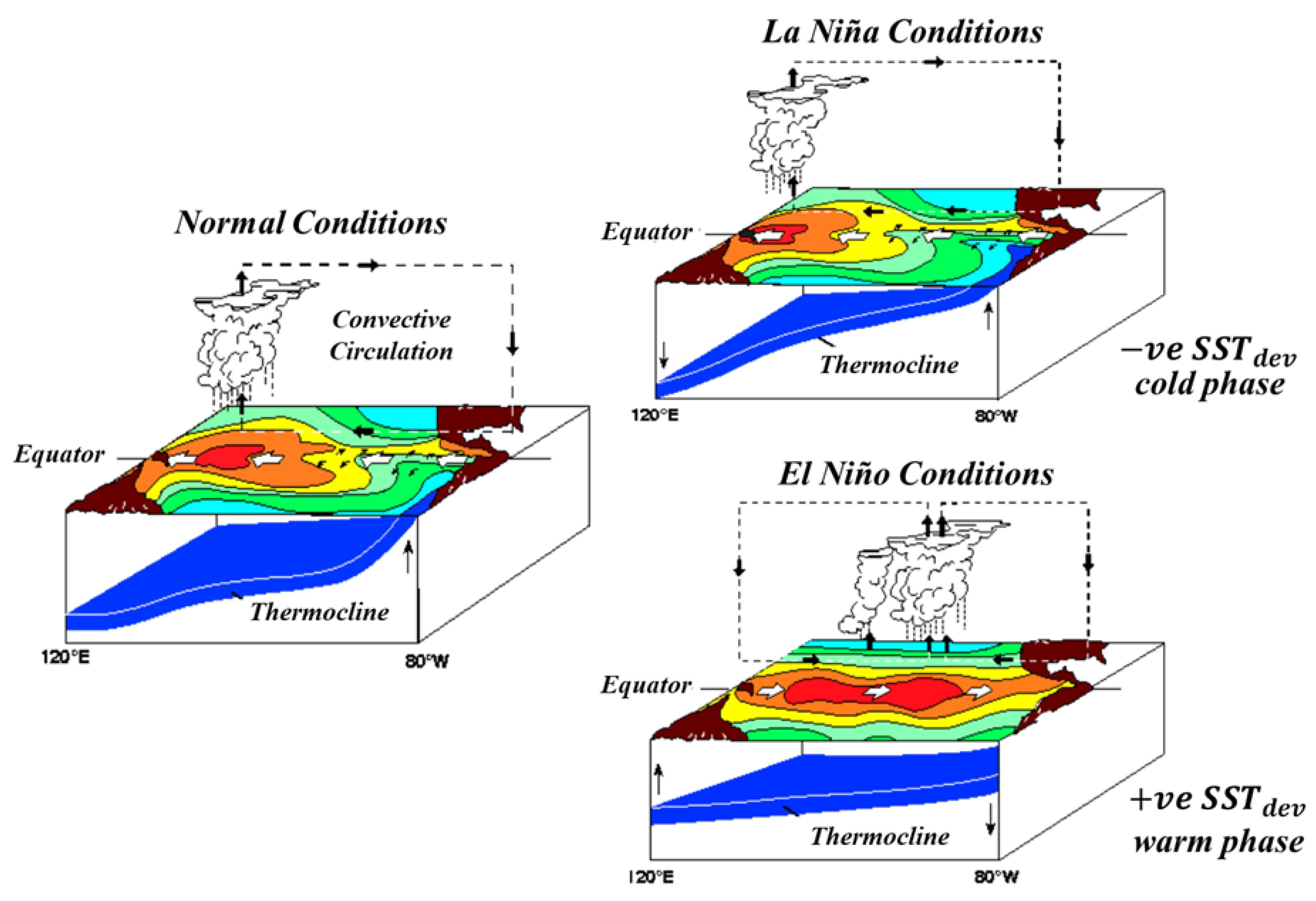
6. El Niño–Southern Oscillation

El Niño, in its original sense, is a warm water current that periodically flows along the coast of Ecuador and Peru, disrupting the local fishery. This oceanic event is associated with a fluctuation of an inter-tropical surface pressure pattern and circulation in the Indian and Pacific oceans, called the Southern Oscillation (SO). This coupled atmosphere–ocean phenomenon is collectively known as the El Niño–Southern Oscillation, or ENSO. During an El Niño event, the prevailing trade winds weaken and the equatorial counter-current strengthens, causing warm surface waters in the Indonesian area to flow eastward to overlie the cold waters of the Peru current. This event has great impact on the wind, sea surface temp, and precipitation patterns in the tropical Pacific. It has climatic effects throughout the Pacific region and in many other parts of the world. The opposite of an El Niño event is called La Niña (see the details in [26,27,28,29,30]).

The Christ Child was first recognized as a warm surface counter-current flowing down the Ecuadorian and Peruvian coasts around Christmastime and, thus, was named by local fishermen. Discovered for the first time in 1795. El Niños were most recent and severe in 1953, 1957–1958, 1965, 1972–1973, 1976–1977, 1982–1983, 1987–1988, 1997–1998, and 2002–2003. El Niño is cyclical, implying it occurs in cycles. Jacob Bjerknes (1969) demonstrated using the most recent wind, rain, and sea surface temperature (SST) data that the Southern Oscillation and El Niño are not distinct phenomena (abbreviated as ENSO). El Niño’s effects are not limited to Peru, but could affect the entire Pacific and even the entire world (see the details in [26,27,28,29,30]).

During a La Niña event, the eastern Pacific remains colder than the western Pacific and the atmospheric pressure in the east is higher than in the west, so the wind blows (trade wind) from east to west and pushes warm surface water and vapor to the west, and the heated rising air over the western Pacific causes rainfall in the west. On the other hand, during an El Niño event, the eastern Pacific becomes warmer, the trade wind becomes weak, and an opposing wind from west to east begins, so the wind blows from west to east and pushes warm surface water and vapor to the east, and the heated rising air over the eastern Pacific causes rainfall in the east (see Figure 13) (see the details in [26,27,28,29,30]).

7. Aspects of Land Surface Climate

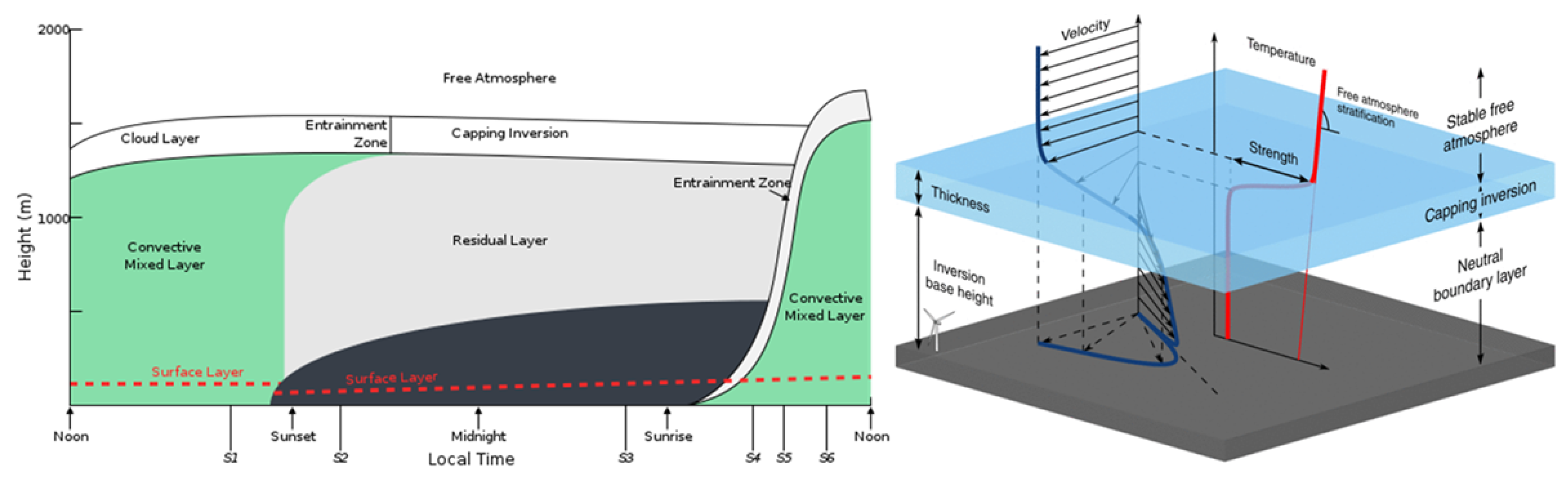
Planetary Boundary Layer

The air close to the ground is more turbulent than the air at higher altitudes. Low-level turbulence is least during the night, occurring solely as a result of mechanical stirring of rough surfaces, and is highest in the afternoon, occurring as a result of heat convection and, hence, more vigorous stirring. Because atmospheric pressure falls with altitude, stirring an atmospheric layer cools increasing parcels of air by adiabatic expansion and warms sinking parcels via compression. The temperature decreases at a rate of 9.8 ${}^{°}$C per Km, which is referred to as the adiabatic lapse rate (g/$C_p$), where the $Cp$ specific heat of the atmosphere at constant pressure equals 1004 J/K/Kg. The atmospheric layer immediately above the surface is sufficiently mixed to sustain a lapse rate close to or slightly greater than the adiabatic; this is referred to as the planetary boundary layer. Above the planetary boundary layer, the atmosphere is generally very stable (i.e., environmental lapse rate < adiabatic lapse rate) due to latent heat released during condensation and precipitation, as well as upward heat transmission via large-scale atmospheric motion. In high-pressure zones over land, the planetary boundary layer is composed of three principal components: (1) a highly turbulent mixed layer, (2) a less-turbulent residual layer containing former mixed-layer air, and (3) a nighttime stable boundary layer with intermittent turbulence; the mixed layer is further differentiated into a cloud layer and a subcloud layer (see Figure 14) [36].

8. Climate Variability

Climate variability is the deviation of climate characteristics (such as temperature and precipitation) from the mean. Natural and sometimes periodic changes in air and ocean circulation, volcanic eruptions, and other factors cause climate variability. The average global temperature rarely remains constant from one year to the next. One year may be cooler than the previous year, despite the long-term trend of rising temperatures due to climate change. There are numerous causes of climate variability, such as natural changes such as the ENSO. For example, the Great Plains droughts of the 1930s and 1950s, and the Sahelian rainfall shortfall of the 1960s. Volcanoes and solar variability may possibly play a role (though their significance is still debatable); it has proven difficult to substantiate links between drought and the 11-year sunspot cycle or the 22-year solar magnetic variation. Currently, scientists are investigating the effect that climate change has on variability [38].

8.1. Small-Scale Climate Variability

Due to a variety of local controls, the climate of a small area can differ significantly from that of the larger surrounding region. Local differences in terrain, land surface characteristics, and air pollution all affect airflow, cloudiness, temperature, and even precipitation via their effects on surface roughness, heat, and water balance. Topography influences both mesoscale and microscale climate variations; regionally, mountain ranges force ascent for wind, condensation, and heavy precipitation, while subsiding air is relatively dry, resulting in a rain shadow effect thousands of km below; for example, the Rocky Mountains channel large-scale outflows of cold air from the polar regions; elevation affects temperature and precipitation type due to the atmospheric lapse rate (which decrease at a rate of 9.8 ${}^{°}$C/km); elevation affects temperature and precipitation type. At one extreme, the summer afternoon lapse rate over arid regions may be nearly dry adiabatic down to several thousand meters; at the other extreme, a strong low-level temperature inversion frequently forms at night over middle- and high-latitude continents during winter under clear skies and light winds (see the details in [26,27,28,29,30]).

Local wind systems are prevalent in a wide variety of environments; they can be gravity-driven in mountainous regions and off ice fields and glaciers; thermally driven by differential surface heating; or mechanically driven by isolated hills or mountains. Local thermal circulations are most prominent in the tropics and middle latitudes during the warmer months, when large-scale temperature gradients and circulation are weak; thermally driven diurnal wind systems include mountain–valley winds, land–lake and land–sea breezes, and urban–rural contrasts (see the details in [26,27,28,29,30]).

Climate varies in part due to topographic bias (e.g., in valleys), but mostly due to different land characteristics and air quality, a phenomena known as the heat island effect, which causes a higher nighttime temperature.

Due to the large heat capacity of water, seasonal changes in water temperature lag behind those on land; water is cooler in the spring and early summer than land and warmer in the fall and early winter; this causes land–lake wind impacts to vary seasonally (see the details in [26,27,28,29,30]).

8.2. Drought

This is generally associated with a sustained period of decreased soil moisture and water supply in comparison to the normal levels that have stabilized the local environment and society. Humidity is a rare and disruptive feature. Semiaridity is common and frequently catastrophic, and desert is a meaningless concept. Drought is defined by the following criteria: precipitation, evapotranspiration, streamflow, runoff, groundwater levels, water supply, and water needs (see the details in [26,27,28,29,30]).

The most frequently used definitions of drought are as follows: Drought is defined meteorologically as a period of time, typically months or years, during which the actual supply of moisture at a given location falls cumulatively short of the climatologically appropriate supply. Drought is defined in agriculture as a period of insufficient soil moisture to meet the evapotranspiration demand required to initiate and sustain crop growth. Hydrologic drought refers to periods of reduced streamflow and/or depleted reservoir storage. Economic drought is caused by physical processes, but it primarily affects the economic sectors of human activity. Understanding the factors affecting the time scales, amplitudes, and frequency of droughts provides insight into the physical processes (most notably ocean–atmosphere interaction) that validate drought regimes (see the details in [26,27,28,29,30]).

9. Greenhouse Effect and Global Warming

9.1. Greenhouse Effect

The first speculation that a greenhouse effect might occur was by the Swedish chemist Svante Arrhenius in 1897. The Sun radiates vast quantities of energy into space, across a wide spectrum of wavelengths.

Most of the radiant energy from the Sun is concentrated in the visible part of the spectrum. The narrow band of visible light, between 400 and 700 nm, represents 43% of the total radiant energy emitted. Wavelengths shorter than the visible account for 7 to 8% of the total, but are extremely important because of their high energy per photon. The shorter the wavelength of light, the more energy it contains. Thus, ultraviolet light is very energetic (capable of breaking apart stable biological molecules and causing sunburn and skin cancers). The remaining 49–50% of the radiant energy is spread over the wavelengths longer than those of visible light. Various components of Earth’s atmosphere absorb ultraviolet and infrared solar radiation before it penetrates to the surface, but the atmosphere is quite transparent to visible light (see the details in [39,40]).

Absorbed by land, oceans, and vegetation at the surface, the visible light is transformed into heat and re-radiates in the form of invisible infrared radiation. The Earth’s atmosphere contains molecules that absorb the heat and re-radiate the heat in all directions. This reduces the heat radiated out to space. The trapping and warming is somewhat analogous to a greenhouse, which also traps heat; thus, the process is called the greenhouse effect (see the details in [39,40]).

In common usage, “greenhouse effect” may refer either to the natural greenhouse effect due to naturally occurring greenhouse gases or to the enhanced (anthropogenic) greenhouse effect that results from gases emitted as a result of human activities (see the details in [39,40]).

9.2. Natural Greenhouse Effect

Without the greenhouse gases, during the day, Earth would heat up, but at night, all the accumulated energy would radiate back into space and the planet’s surface temperature would fall far below zero very rapidly. The reason this does not happen is that Earth’s atmosphere contains greenhouse gases that absorb the heat and re-radiate the heat in all directions. This reduces the heat radiated out to space (see the details in [39,40]).

9.3. Anthropogenic Greenhouse Effect

Human activities are in part responsible for the increase in some greenhouse gases, and this causes an enhanced greenhouse effect (and as a result, global warming). About three-quarters of the anthropogenic (man-made) emissions of carbon dioxide to the atmosphere during the past 20 years are due to fossil fuel burning. The rest of the anthropogenic emissions are predominantly due to land-use change, especially deforestation (see the details in [39,40]).

9.4. Greenhouse Gases

Greenhouse gases (GHGs) are gaseous components of the atmosphere that contribute to the “greenhouse effect”. Although uncertainty exists about exactly how Earth’s climate responds to these gases, global temperatures are rising (global warming). Some greenhouse gases occur naturally in the atmosphere, while others result from human activities. Naturally occurring greenhouse gases include water vapor, carbon dioxide, methane, nitrous oxide, and ozone. Certain human activities, however, add to the levels of most of these naturally occurring gases. The major natural greenhouse gases are water vapor, which causes about 36–70% of the greenhouse effect on Earth (not including clouds); carbon dioxide, which causes 9–26%; methane, which causes 4–9%; and ozone, which causes 3–7%. Other greenhouse gases include, but are not limited to, nitrous oxide, sulfur hexafluoride, hydrofluorocarbons, perfluorocarbons, and chlorofluorocarbons (CFCs). The major components of the atmosphere (N${}_2$ and O${}_2$) are two-atom molecules too tightly bound together to vibrate, and thus, they do not absorb heat and contribute to the greenhouse effect (see the details in [39,40]).

We are not particularly worried about water vapor in the future because it is not significantly increasing in the atmosphere as a result of human-induced (i.e., anthropogenic) processes. Anthropogenic GHGs include carbon dioxide, CFCs, methane, and nitrous oxide, all of which have increased significantly in the atmosphere in recent years (see the details in [39,40]).

9.4.1. Water Vapor

Water vapor is a natural greenhouse gas and accounts for the largest percentage of the greenhouse effect. Water vapor concentrations fluctuate regionally, but human activity does not directly affect water vapor concentrations except at very local scales (see the details in [39,40]).

9.4.2. Carbon Dioxide

About 50% to 60% of the anthropogenic greenhouse effect is attributed to carbon dioxide. The measurement of carbon dioxide trapped in air bubbles in Antarctic ice sheet suggests that, during the 160,000 years prior to the industrial revolution, the atmospheric concentration of carbon dioxide varied from approximately 200 to 300 ppm. At the beginning of the industrial revolution, the atmospheric concentration of carbon dioxide was approximately 280 ppm. Today, the concentration of carbon dioxide in the atmosphere is approaching 370 ppm, and it is predicted that the level may rise to 450 ppm by the year 2050. Currently, the rate of increase of carbon dioxide in the atmosphere is about 0.5% per year (see the details in [39,40]).

The high rate of carbon dioxide emissions and the high growth rate of the emissions would seem to suggest that the increase in carbon dioxide in the atmosphere is a direct result of the anthropogenic input of carbon dioxide from sources such as burning fossil fuels and deforestation. It is a reasonable hypothesis that these increases will continue to contribute to global warming via the greenhouse effect (see the details in [39,40]).

Increased atmospheric carbon dioxide increases the amount of CO${}_2$ dissolved in the oceans. This decreases the greenhouse effect by removing the greenhouse gas from the atmosphere. Unfortunately, carbon dioxide gas dissolved in the ocean reacts with water to form carbonic acid. The net effect, even accounting for warming of the oceans, is an observed and accelerating ocean acidification. Since bio-systems are adapted to a narrow range of $pH$, this is a very serious concern directly driven by increased atmospheric CO${}_2$ (see the details in [39,40]).

The Keeling Curve is a graph of the accumulation of CO${}_2$ in the Earth’s atmosphere from 1958 to the present, as determined by continuous observations obtained at the Mauna Loa Observatory on the island of Hawaii. The curve is named after the scientist Charles David Keeling, who initiated and oversaw the monitoring program until his passing in 2005 [41].

The increased CO${}_2$ in the atmosphere absorbs shortwave radiation, which warms the Earth’s surface and leads to melting of ice near the poles, which in turn contributes to the sea level rise (see the details in [39,40]).

9.4.3. Methane

Until 1991, methane was increasing in the atmosphere at a rate of approximately 1% per year, and it is thought to contribute approximately 12% to 20% of the anthropogenic greenhouse effect (see the details in [39,40]).

Natural environments release methane into the atmosphere. Major contributors are termites, which produce methane as they process wood, and freshwater wetlands, where decomposing plants in oxygen-poor environments produce and release methane as a decay product (see the details in [39,40]).

The several anthropogenic sources of methane include the burning of biomass (organic material such as logs) and agricultural activities, such as the cultivation of rice and the raising of cattle. Methane is released by anaerobic activity in the flooded lands where rice is grown, and cattle expel methane gas as part of their digestive processes (see the details in [39,40]).

9.4.4. CFCs

It has been estimated that approximately 15% to 25% of the anthropogenic greenhouse effect may be related to CFCs in the atmosphere. The rate of growth of CFCs in the atmosphere in recent years has been 5% per year (see the details in [39,40]).

CFCs are highly stable compounds that are used in spray cans as aerosol propellants, refrigeration units, air conditioning, and fire extinguishers (see the details in [39,40]).

The potential global warming from CFCs is considerable, because each CFC molecule may absorb hundreds- or even several-thousand-times more infrared radiation emitted from Earth than is absorbed by a molecule of carbon dioxide (see the details in [39,40]).

9.4.5. Nitrous Oxide

Nitrous oxide (N${}_2$O) is also increasing in the atmosphere and is probably contributing as much as 5% of the anthropogenic greenhouse effect (see the details in [39,40]).

Anthropogenic sources of nitrous oxide include agricultural activities (application of fertilizer) and burning of fossil fuels (see the details in [39,40]).

9.5. Global Warming

Global warming is defined as a natural or human-induced increase in the average global temperature of the atmosphere near the Earth’s surface.

Potential Effects of Global Warming

Climatic changes are likely to occur by the year 2030 owing to the doubling of carbon dioxide in the atmosphere since the industrial revolution. Global warming is expected to result in wetter winters, hotter and drier summers, an increased frequency of large storm events, and a rise in sea level.

In central North America, warming is expected to vary from approximately 2 ${}^{°}$C to 4 ${}^{°}$C, with an increase in winter precipitation (see the details in the next section), but a decrease in summer rains. As a result, soil moisture is expected to decrease in the summer by as much as 20% (see the details in [39,40]).

There is also concern that global warming will alter normal weather and climatic patterns, including a change in the frequency or intensity of violent storms. The hypothesis is that warming ocean waters could feed more energy into high-magnitude storms, such as cyclones and hurricanes, causing a significant increase in their frequency or intensity.

The expansion of tropical climate zones expected in global warming will lead to an increase in tropical diseases such as malaria, dengue fever, yellow fever, and viral encephalitis.

A rise in sea level is a potentially serious problem as it relates to global warming. The causes for the rise in sea level due to global warming are thought to be twofold: thermal expansion of warming ocean water (primary cause) and melting of glacial ice (secondary cause). The various models predict that the rise may be anywhere from 20 cm to approximately 2 m in the 21st Century. It could easily cause increased coastal erosion on open beaches, thus making buildings and other structures in the coastal zone more vulnerable to damage from waves generated by high-magnitude storms. It could also cause a landward migration of estuaries and salt marshes, putting additional pressure on human structures in the coastal zone. Additionally, groundwater supplies for coastal communities may be threatened by saltwater intrusion should sea levels rise (see the details in [39,40]).

Global warming and, consequently, sea level rise will have a far-reaching effect on Sundarbans located in the southern part of Bangladesh. The Sundarbans, one of the world’s richest mangrove forests, would disappear, leading to a major loss in biodiversity, the loss of a natural sink for greenhouse gases, and the loss of biomass that is a major energy source in the country.

10. The Pillars of Climate Change

2019 was the hottest year on record occurred in the last 20 years. Compared to global average temperatures from 1950–1980, the world today is about 0.85 ${}^{°}$C or 1.5 ${}^{°}$F higher. Based on climate models’ projections, in another 40 years, these temperatures will increase by another 1.5 ${}^{°}$C or 2.7 ${}^{°}$F. One degree of temperature increase in global energy retention is literally an astronomical number. A one-degree increase means that just the atmosphere contains 5 × 10${}^{18}$ KJ more energy [42,43,44,45,46,47,48]. However, for a few meters of the ocean likely achieving equilibrium with the atmosphere, this energy retention number doubles. In fact, this exceeds the energy contained in all known oil reserves on the planet. In other words, this increase in retained energy is the source of chaos. More water evaporates from the oceans, resulting in more intense precipitation in certain regions of the globe. It increases the intensity of hurricanes, resulting in greater damage to coastal areas. Warmer water expands in volume, and more polar ice melts, causing sea levels to rise.

However, the Earth has experienced numerous temperature cycles in the past, so it is the subject of debate whether this change is normal or not [42]. To discuss climate, we must first agree on the definition of climate. The short-term climate does not reveal much about the global climate’s long-term trends. As discussed earlier, climate is typically measured over a period of more than 30 years. It describes a general trend over a long period of time in particular places. An increase in global average temperatures is an average. There are parts of the world that will warm less, and some will warm much more; however, some rare areas might also cool. Parts of Southern Africa for example are warming about 2 ${}^{°}$C, and the Arctic appears to be warming 4 ${}^{°}$C, while the southern tip of Greenland is cooling [18]. Temperature trends across the globe are not uniform because of the diverse geography of Earth. Scientists have calculated the global average temperature, and they have reached the conclusion that the climate is indeed changing [42].

This can be understood using a straightforward principle. Extreme weather causes havoc, which indicates that it imparts energy or performs work. In physics, work can be expressed as a simple change in kinetic energy. In other words, energy is required to cause any type of weather damage. For the wind to act on the Earth and cause storms or tornadoes, it requires energy. The Sun is the source of this energy. Almost all energy on Earth is derived from the Sun in some fashion. When the Sun heats the Earth, unequal heating results. Over land, the air is drier and warms up more rapidly than over water. This is due to the fact that the specific heat capacity of water is significantly greater than that of land, meaning that it requires more energy to heat the sea than the land; consequently, the sea is typically cooler than the land. This indicates that land is significantly warmer than water. As with hot air balloons, hot air rises because its density is less than that of cold air. However, as the air from the land rises to form clouds, colder air from the ocean fills the void, causing a breeze or wind. In contrast to the cool air over the ocean, which has a high-pressure zone, hot air has a low density, resulting in a low-pressure zone. From high pressure to low pressure, air flows. This results in wind. If the pressure difference is very great, the wind can be extremely powerful. In order to complete the cycle, the rising hot air in the atmosphere is eventually pushed to the ocean, where it cools, and the cycle continues [42].

Due to global warming, the Sun heats the Earth more, resulting in a greater pressure difference between the sea and the land. As a result, winds can become more intense, leading to more severe weather. As a result of the Sun’s influence on the water cycle, we also experience more intense precipitation. As a result of the Sun’s heating of the ocean, water evaporates, and then, when air containing that water vapor is cooled, the water vapor condenses out, forming clouds. Eventually, these clouds grow larger, and the precipitating water falls as rain, hail, or snow. This cycle is accelerated by global warming, resulting in more precipitation in areas where it rains. In regions where there is insufficient precipitation and where temperatures are rising, droughts occur because the little water present evaporates and there is insufficient rainfall to compensate. This means that certain regions of the planet will experience more hail, more snow, more drought, stronger winds, and so on. Therefore, global warming involves not only warmer weather, but also more extreme weather. That can be hazardous for us humans, not to mention all other species in the natural environment [42].

As described earlier, the Sun is the driving force behind both the climate and life on Earth. Therefore, one could argue that the higher temperatures of today are the result of a warming Sun. However, computer models demonstrate that this is almost certainly not the case, as the variation in total irradiance over 11 years is only 0.15% [42,49,50]. On the other hand, the temperature on Earth has changed many times in Earth’s history going back millions of years. Earth’s rotation around the Sun slowly changes over tens of thousands of years, causing cycles of ice ages and warm periods. The last ice age ended about 11 thousand years ago [42,49,50,51]. However, Earth has been much hotter; in fact, 56 million years ago, Earth warmed by 5–8 ${}^{°}$C. At that time, Earth was experiencing extreme warming called the Paleo-Eocene thermal maximum (or $PETM$). The problem is that extreme warming cycles such as the $PETM$ have been a complete disaster for life on Earth. Deep sea organisms went extinct. Oceans acidified. Much of the land mass either went underwater or was uninhabitable by our mammalian ancestors due to excessive heat or humidity [42,49,50,51]. Now, scientists have determined that this is the event most similar to what we are currently experiencing. Extensive research is being conducted to inform us of what we may face in the near future. There are a number of similarities, as well as differences, with the current warming [42]. The $PETM$ was also initiated by huge increases in carbon dioxide in the atmosphere. As discussed earlier, greenhouse gases, including carbon dioxide, water vapor, and methane, each have at least three atoms in their molecules. The atoms in these molecules are loosely held and can absorb more vibrational energy. They are efficient at absorbing light in the long-wave range, which is also called heat, which bounces up from the Earth’s surface. These greenhouse gases then re-emit this long-wave radiation back toward Earth’s surface, resulting in warming. Other non-greenhouse gases such as oxygen and nitrogen do not absorb the long-wave radiation, and so, the heat passes through them and into space instead of being reflected back to Earth. However, there were no humans during the $PETM$, so fossil fuel combustion could not have caused this. This enormous amount of CO${}_2$ going into the atmosphere was probably caused by volcanic eruptions [42,52]. Many series of eruptions over thousands of years caused it. The evidence for this can be found in the fossil record, as well as carbon-dated rocks that show a significant increase in Carbon 13, which is the isotope of carbon most prevalent in volcanic eruptions. It is estimated that, on average, about a net 0.24 gigatons of carbon was emitted into the atmosphere during a 50,000-year period to cause this severe warming known as the $PETM$ [42,49,50,51,52]. In comparison, humans emit 10 gigatons, or approximately fifty-times that amount of carbon annually, into the atmosphere. Moreover, the current 1-degree warming has occurred in less than 100 years, not over thousands of years. The most convincing evidence comes from carbon isotopes in the atmosphere. Fossil fuels are derived from ancient plants with a higher ratio of $C12$ to $C13$ than the atmosphere. $C12$ levels rise as fossil fuels are depleted. Therefore, $C12/C13$ should increase. The data support this. Eruptions of volcanism increase $C13$, not $C12$. Volcanoes emit 1% of human carbon dioxide. Thus, they are not responsible. If the Sun were responsible for global warming, it would warm both the upper and lower atmospheres of the planet. However, only the lower atmosphere, where greenhouse gases accumulate, is warming. In addition, solar activity over the past 50 years has been sufficient to have lowered the Earth’s temperature on its own. Earth’s natural climate cycles are also unlikely to be to blame, as ice core evidence indicates that the planet warmed at a rate of 0.06 degrees per century at the end of the last ice age. Today, however, we are experiencing at least approximately 0.6 degrees per century. In addition, simulations are conducted using only natural causes of climate change, and neither a warming nor a cooling is predicted for the next two-thousand years. However, if we include the unnatural effects caused by emissions from human-made sources, the model matches the observed results more closely. In addition, when combining natural and anthropogenic effects, the simulation closely matches the observed data when plotted as a whole [53,54]. Furthermore, 97% of climate scientists worldwide concur that humans are the cause of this change. CO${}_2$ emissions are not the only contributor to global warming. Other greenhouse gases, such as methane from farm animals and natural gas processing, as well as nitrous oxide from fertilizers, exacerbate the problem [55]. In addition, add the elimination of natural carbon-absorbing sinks such as forests over the past century, and the consequences become even more severe. In the past century, approximately 20% of the world’s forests have disappeared [56]. Therefore, humans are responsible, and every individual can contribute by reducing his/her own carbon footprint and encouraging others to do the same. We only have one lifeboat. No extra are available. Apathy has more negative effects than denial. Climate change is not likely to result in human extinction. Because these changes will continue to wreak havoc, our true goal is to alleviate human suffering. Life will become progressively more challenging. Planet Earth will endure. It is a white canvas. It does not care what endures or who suffers. Our collective effort is the only thing capable of saving us from ourselves (see the details [42]).

11. Conclusions

The major purpose of this technical note is to acquaint engineers with the foundations of the climate and the processes that govern it so that they are able to properly utilize this information to comprehend the climatic impact on water resource systems.

References

1. NOAA. Climate Prediction Center: Climate Glossary; NOAA: Washington, DC, USA, 2010.
2. Brekke, L.D. Climate Change and Water Eesources Management: A Federal Perspective; Diane Publishing: Darby, PA, USA, 2009. [Google Scholar]
3. Oliver, J.E. Encyclopedia of World Climatology; Springer Science & Business Media: Berlin/Heidelberg, Germany, 2008. [Google Scholar]
4. Sarker, S.; Veremyev, A.; Boginski, V.; Singh, A. Critical nodes in river networks. Sci. Rep. 2019, 9, 1–11. [Google Scholar] [CrossRef] [Green Version]
5. Sarker, S. Investigating Topologic and Geometric Properties of Synthetic and Natural River Networks under Changing Climatic. Ph.D. Thesis, University of Central Florida, Orlando, FL, USA, 2021. [Google Scholar]
6. Gao, Y.; Sarker, S.; Sarker, T.; Leta, O.T. Analyzing the critical locations in response of constructed and planned dams on the Mekong River Basin for environmental integrity. Environ. Res. Commun. 2022, 4, 101001. [Google Scholar] [CrossRef]
7. Lee, C.; Sheridan, S. Synoptic Climatology: An Overview. Reference Module in Earth Systems and Environmental Sciences; Elsevier: Amsterdam, The Netherlands, 2015. [Google Scholar]
8. NOAA. National Centers for Environmental Information: What’s the Difference between Weather and Climate? Available online: https://www.ncei.noaa.gov/news/weather-vs-climate#:~:text=Whereas%20weather%20refers%20to%20short,time%20in%20a%20specific%20area (accessed on 2 March 2022).
9. Sarker, S. A Short Review on Computational Hydraulics in the context of Water Resources Engineering. Open J. Model. Simul. 2022, 10, 1–31. [Google Scholar] [CrossRef]
10. Sarker, S. Essence of MIKE 21C (FDM Numerical Scheme): Application on the River Morphology of Bangladesh. Open J. Model. Simul. 2022, 10, 88–117. [Google Scholar] [CrossRef]
11. NASA. What’s the Difference between Weather and Climate? Available online: https://www.nasa.gov/mission_pages/noaa-n/climate/climate_weather.html (accessed on 3 March 2022).
12. Barry, R.G.; Gan, T.Y. The Global Cryosphere: Past, Present, and Future; Cambridge University Press: Cambridge, UK, 2022. [Google Scholar]
13. Chen, B. Coupled Terrestrial Carbon and Water Dynamics in Terrestrial Ecosystems: Contributions of Remote Sensing. In Remote Sensing: Applications; InTech: Rijeka, Croatia, 2012; p. 223. [Google Scholar]
14. NCCO. Earth’s Energy Balance. Available online: https://legacy.climate.ncsu.edu/edu/EnergyBalance (accessed on 4 March 2022).
15. Chow, V.T.; Maidment, D.R.; Larry, W.M. Applied Hydrology; International Edition; MacGraw-Hill Inc.: New York, NY, USA, 1988; Volume 149. [Google Scholar]
16. Ames, I.A. Carbon Sequestration and Greenhouse Gas Fluxes in Agriculture: Challenges and Opportunities; Council for Agricultural Science and Technology: Ames, IA, USA, 2011. [Google Scholar]
17. NASA-FAU. The Sun’s Electromagnetic Spectrum. Available online: http://www.ces.fau.edu/nasa/module-2/radiation-sun.php (accessed on 3 March 2022).
18. Sarker, T. Role of Climatic and Non-Climatic Factors on Land Use and Land Cover Change in the Arctic: A Comparative Analysis of Vorkuta and Salekhard. Master’s Thesis, The George Washington University, Washington, DC, USA, 2020. [Google Scholar]
19. NASA. Earth’s Upper Atmosphere. Available online: https://www.nasa.gov/mission_pages/sunearth/science/mos-upper-atmosphere.html (accessed on 8 March 2022).
20. NUS. Principles of Remote Sensing; Centre for Remote Imaging, Sensing and Processing, National University of Singapore: Singapore, 2001. [Google Scholar]
21. Bryant, E.; Bryant, E.A.; Edward, B. Climate Process and Change; Cambridge University Press: Cambridge, UK, 1997. [Google Scholar]
22. NASA. Earth Observatory: Heating Imbalances. Available online: https://earthobservatory.nasa.gov/features/EnergyBalance/page3.php (accessed on 14 March 2022).
23. NOAA. Global Circulations. 2022. Available online: https://www.noaa.gov/jetstream/global/global-circulations (accessed on 14 March 2022).
24. UCAR. A Global Look at Moving Air: Atmospheric Circulation. Available online: https://scied.ucar.edu/learning-zone/how-weather-works/global-air-atmospheric-circulation (accessed on 14 March 2022).
25. Nugent, A.; DeCou, D.; Russell, S.; Karamperidou, C. Atmospheric Processes and Phenomena; UH Pressbooks, The University of Hawaii: Honolulu, HI, USA, 2019. [Google Scholar]
26. Hidore, J.J.; Oliver, J.E. Climatology: An Atmospheric Science; MacMillan Publishing Co.: New York, NY, USA, 1993. [Google Scholar]
27. Wang, S.Y.S.; Gillies, R. Modern Climatology; BoD–Books on Demand: Norderstedt, Germany, 2012. [Google Scholar]
28. Miller, A.A. Climatology; Routledge: Abingdon-on-Thames, UK, 2019. [Google Scholar]
29. Perry, A.; Thompson, R. Applied Climatology: Principles and Practice; Routledge: Abingdon-on-Thames, UK, 2013. [Google Scholar]
30. Hobbs, J.E. Applied Climatology: A Study of Atmospheric Resources; Elsevier: Amsterdam, The Netherlands, 2016. [Google Scholar]
31. Akbari, E.; Alavipanah, S.K.; Jeihouni, M.; Hajeb, M.; Haase, D.; Alavipanah, S. A review of ocean/sea subsurface water temperature studies from remote sensing and non-remote sensing methods. Water 2017, 9, 936. [Google Scholar] [CrossRef] [Green Version]
32. NASA (PennState). The Global Conveyor Belt. Available online: https://www.e-education.psu.edu/earth103/node/686 (accessed on 15 May 2022).
33. Wang, C. Three-ocean interactions and climate variability: A review and perspective. Clim. Dyn. 2019, 53, 5119–5136. [Google Scholar] [CrossRef]
34. NOAA. The Global Conveyor Belt. Available online: https://oceanservice.noaa.gov/education/tutorial_currents/05conveyor2.html (accessed on 15 May 2022).
35. NOAA. Normal Pacific Pattern, El Niño Conditions and La Niña Conditions; NOAA: Washington, DC, USA, 2014.
36. Salby, M.L. Fundamentals of Atmospheric Physics; Elsevier: Amsterdam, The Netherlands, 1996. [Google Scholar]
37. Reijs, V. Atmosphere Boundary Layers Influencing Atmospheric Refraction. Available online: http://www.archaeocosmology.org/eng/tropospherelayers.htm (accessed on 15 May 2022).
38. UCAR. Climate Variability. Available online: https://scied.ucar.edu/learning-zone/how-climate-works/climate-variability (accessed on 15 May 2022).
39. EPA. Basics of Climate Change. Available online: https://www.epa.gov/climatechange-science/basics-climate-change#:~:text=The%20greenhouse%20effect%20helps%20trap,the%20earth%20to%20warm%20up (accessed on 15 May 2022).
40. NASA. Global Climate Change: What Is the Greenhouse Eeffect? Available online: https://climate.nasa.gov/faq/19/what-is-the-greenhouse-effect/ (accessed on 18 May 2022).
41. UCSanDiego. The Keeling Curve. Available online: https://keelingcurve.ucsd.edu/ (accessed on 20 May 2022).
42. Ash, A. What’s the Real Cause of Climate Change? What the Deep Data Reveals. 2022. Available online: https://www.youtube.com/watch?v=-skE4jCuf-w&t=22s (accessed on 22 June 2022).
43. Roston, E.; Migliozzi, B. What’s Really Warming the Word? 2015. Available online: https://www.bloomberg.com/graphics/2015-whats-warming-the-world/ (accessed on 22 June 2022).
44. Kennedy, C. Why Did Earth’s Surface Temperature Stop Rising in the Past Decade? 2018. Available online: https://www.climate.gov/news-features/climate-qa/why-did-Earth%E2%80%99s-surface-temperature-stop-rising-past-decade (accessed on 22 June 2022).
45. UCAR. Why Earth Is Warming. Available online: https://scied.ucar.edu/learning-zone/how-climate-works/why-Earth-warming (accessed on 22 June 2022).
46. NASA. Global Temperature. Available online: https://climate.nasa.gov/vital-signs/global-temperature/ (accessed on 22 June 2022).
47. Our World in Data: Energy Mix. Available online: https://ourworldindata.org/energy-mix#:~:text=Globally%20we%20get%20the%20largest,still%20dominated%20by%20fossil%20fuels (accessed on 22 June 2022).
48. Scott, M.; Lindsey, R. What’s the Hottest Earth’s Ever Been? 2020. Available online: https://www.climate.gov/news-features/climate-qa/whats-hottest-earths-ever-been (accessed on 22 June 2022).
49. NASA. Sun-Earth. Available online: https://www.nasa.gov/mission_pages/sunearth/solar-events-news/Does-the-Solar-Cycle-Affect-Earths-Climate.html (accessed on 22 June 2022).
50. NASA. Graphic: Temperature vs. Solar Activity. Available online: https://climate.nasa.gov/climate_resources/189/graphic-temperature-vs-solar-activity/ (accessed on 22 June 2022).
51. NASA. Ancient Climate Events: Paleocene Eocene Thermal Maximum. Available online: https://www.e-education.psu.edu/earth103/node/639 (accessed on 22 June 2022).
52. Pappas, S. Carbon Dioxide Is Warming the Planet (Here’s How). 2017. Available online: https://www.livescience.com/58203-how-carbon-dioxide-is-warming-Earth.html (accessed on 22 June 2022).
53. NASA. Earth Observatory: Is Current Warming Natural? Available online: https://earthobservatory.nasa.gov/features/GlobalWarming/page4.php#:~:text=When%20the%20Sun’s%20energy%20is,but%20the%20stratosphere%20has%20cooled (accessed on 22 June 2022).
54. NASA. Earth Observatory: How is Today’s Warming Different from the Past? Available online: https://earthobservatory.nasa.gov/features/GlobalWarming/page3.php#:~:text=As%20the%20Earth%20moved%20out,ice-age-recovery%20warming (accessed on 22 June 2022).
55. EPA. Overview of Greenhouse Gases. Available online: https://www.epa.gov/ghgemissions/overview-greenhouse-gases (accessed on 22 June 2022).
56. Our World in Data: The World Has Lost One-Third of Its Forest, but an End of Deforestation is Possible. Available online: https://ourworldindata.org/world-lost-one-third-forests (accessed on 22 June 2022).
Figure 1. Schematic view of the components of the global climate system [13].
Eng 03 00040 g001
Figure 2. Radiation and heat balance in the atmosphere and Earth’s surface (global average components of the Earth’s energy balance) [15].
Eng 03 00040 g002
Figure 3. The Earth’s annual and global mean energy balance [16].
Eng 03 00040 g003
Figure 4. Electromagnetic spectrum of the Sun [17].
Eng 03 00040 g004
Figure 5. Radiation balance at the surface [15].
Eng 03 00040 g005
Figure 6. Atmosphere and vertical thermal structure of the Earth [20].
Eng 03 00040 g006
Figure 7. Absorbing solar radiation and emitting long-wave radiation averaged over latitude and atmospheric circulation [23].
Eng 03 00040 g007
Figure 8. Representation of the wind and pressure belts at the surface [23].
Eng 03 00040 g008
Figure 9. Mean meridional circulation of the atmosphere and cyclones.
Eng 03 00040 g009
Figure 10. Global pressure and surface wind for July and January [21].
Eng 03 00040 g010
Figure 11. Ocean temperature and salinity profile [31].
Eng 03 00040 g011
Figure 12. Great ocean conveyor belt [32,33].
Eng 03 00040 g012
Figure 13. El Niño–Southern Oscillation (ENSO) [35].
Eng 03 00040 g013
Figure 14. Planetary boundary layer [37].
Eng 03 00040 g014
Publisher’s Note: MDPI stays neutral with regard to jurisdictional claims in published maps and institutional affiliations.