Abstract
The presented research work demonstrates an efficient methodology based on a micromechanical framework for the prediction of the effective elastic properties of strongly bonded long-fiber-reinforced materials (CFRP) used for the construction of tubular structures. Although numerous analytical and numerical micromechanical models have been developed to predict the mechanical response of CFRPs, either they cannot accurately predict complex mechanical responses due to limits on the input parameters or they are resource intensive. The generalized method of cells (GMC) is capable of assessing more detailed strain fields in the vicinity of fiber–matrix interfaces since it allows for a plethora of material and structural parameters to be defined while being computationally effective. The GMC homogenization approach is successfully combined with the covariance matrix adaptation evolution strategy (CMA–ES) to identify the effective elasticity tensor Cij of CFRP materials. The accuracy and efficiency of the proposed methodology are validated by comparing predicted effective properties with previously measured experimental data on CFRP cylindrical samples made of 3501-6 epoxy matrix reinforced with AS4 carbon fibers. The proposed and validated method can be successively used in both analyzing the mechanical responses of structures and designing new optimized composite materials.
1. Introduction
The use of polymer matrix composites (PMCs) provides significant benefits in the design of advanced lightweight structural systems due to their high strength-to-density ratios. The continuous demand for new, more sophisticated PMCs drives the research on computationally efficient, multiscale design and analysis methodologies, which are critical in the designing and developing of new composite materials for material scientists. Methodologies based on micromechanics theories are fundamental in the modeling of composite materials since in contrast to the macromechanical approach, they provide a material’s mechanical responses to various loading scenarios by considering both the mechanical properties of its constituents and their geometrical arrangement. Thus, composite properties can be determined, in any direction, for any fiber volume fraction or reinforcement architecture, even if the composite has never been manufactured. Micromechanics theories can therefore assist in designing the composite materials themselves as well as the structures they comprise.
Numerous micromechanical models are applied for the estimation of the mechanical response of a structure based on the fundamental properties or responses of its constituents. These techniques can be categorized as simple analytical approximations or more computationally intense, fully numeric methods that require volume discretization. Analytical methods are founded on the concepts of representative volume, average volume, stress and strain, stress and strain concentration tensors, effective thermoelastic properties, and energy considerations. Probably the simplest analytical model is the Voigt–Reuss–Hill (VRH) approximation method [1,2,3]. However, the method, while universal and simple, does not contain information on microgeometry [4]. One modeling approach that allows for describing the interactions between phases or between individual reinforcements is the mean field approach (MFA). A large proportion of MFA descriptions are based on the pioneering work of Eshelby [5] on inclusion and inhomogeneity problems. The simplest MFA is the Mori–Tanaka (MT) theory [6], which encompasses the full physical range of phase–volume fractions and allows for treating composites with high fiber volume fractions. Numerous propositions exist in the literature for extending the applicability of mean field methods to composites ([7,8,9,10]). These propositions are not always successful, especially when the matrix phase has nonlinear responses, and certain engineering-motivated improvements are required [11]. Another group of estimates for the thermomechanical behavior of inhomogeneous materials is the generalized self-consisted scheme (GSCS), which assumes that a single particle (inhomogeneity) surrounded by some matrix material is embedded in an effective medium of unknown properties [12,13,14,15,16]. Although the GSCS has proved its efficiency in numerous situations, it is still limited to lower stiffness ratios ([17,18]). Another major modeling strategy is the periodic microfield approach (PMA), where the behavior is analyzed of infinite (one-, two- or three-dimensional) periodic phase arrangements subjected to far-field mechanical loads. The most common approach to studying the stress and strain fields is the implementation of a repeating unit cell (RUC), which allows for the description of microgeometry [19,20,21,22]. Although the RUC approach uses highly idealized microgeometries, providing only limited information on the microscopic stress and strain fields, these models pose relatively low computational requirements and can be used as constitutive models for analyzing structures made of continuously reinforced composites. The generalized method of cells (GMC) introduced by Paley and Aboudi [23,24] as an extension of the method of cells (MOC) [19] is more flexible geometrically and allows for the finer discretization of RUCs for fiber- and particle-reinforced composites. Fine-grained geometrical descriptions can be obtained using extensive volume discretization with numerical engineering methods, which allows for resolving the micro-stress and strain fields at the length scale of the inhomogeneities. The most popular numerical schemes are finite element methods (FEMs) [25,26,27] and boundary element methods [28,29]. The main disadvantage of these methods is their requirement of significant computational expense to discretize the microgeometry at a prescribed level of accuracy and solve the effective behavior and the local fields.
Herein, a new material design methodology is presented for the assessment of the elastic effective properties of a uniaxial composite material that effectively combines micromechanics theory with a model updating method. The novelty of this work derives from both engineering and computational aspects. From an engineering point of view, the study’s contribution lies on one hand in our in-depth analysis and assessment of the micromechanics analytical theory in efficiently simulating the behavior of the unidirectional CFRP materials used in cylindrical composite structures. On the other hand, the study’s contribution to engineering knowledge also lies in our effective implementation of a novel design methodology for the development of composite material models. This is achieved by effectively combining micromechanics theory with a model updating method, through the coupling of robust GMC to a state-of-the-art covariance matrix adaptation (CMA–ES) optimization algorithm. Furthermore, the study’ novelty from a computational point of view is the applicability of the CMA–ES optimization algorithm to finely tuning both the properties of each material constituent and the geometrical arrangement of a composite laminate component. Thus, the optimized results could be further confidently introduced in subsequent finite-element analysis, introducing user-defined material properties.
This work is organized as follows. The micromechanical modeling methodology is presented in Section 2, along with the GMC to CMA–ES coupling optimization strategy. Section 3 presents the experimental data used in this work to validate the proposed methodology. Section 4 then extensively presents and discusses the results. Finally, Section 5 summarizes the conclusions.
2. Methodology
2.1. Micromechanical Modeling
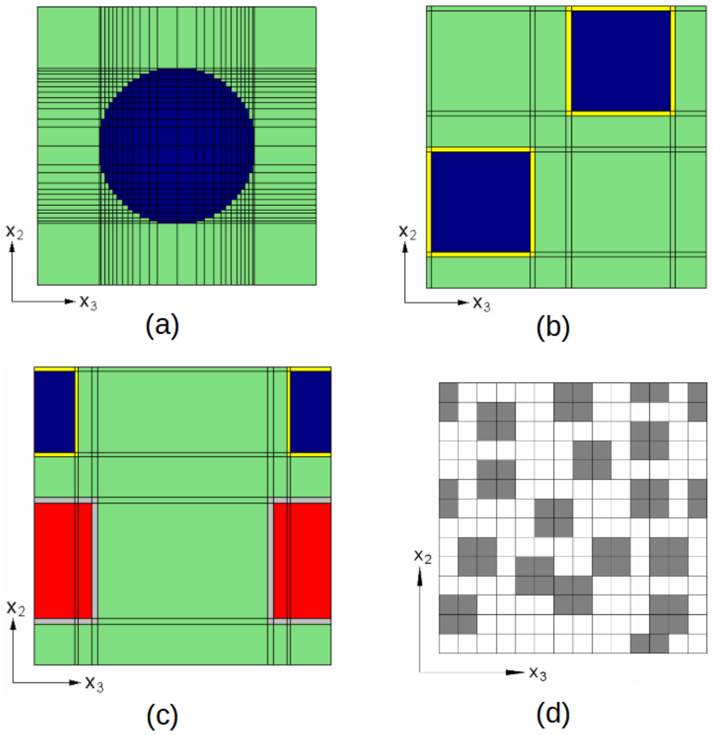
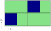
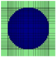
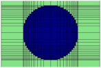
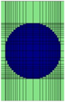
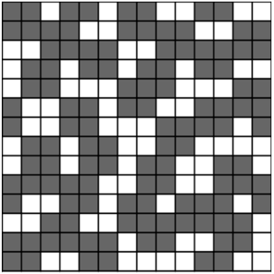
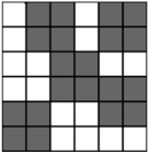
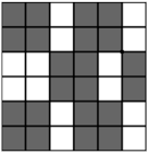
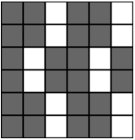
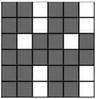
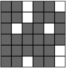
The micromechanical theory of the generalized method of cells (GMC) for continuous or discontinuous fibrous composites was chosen to describe the mathematical links between stress and strain with various levels of idealization. The model was first introduced by Paley and Aboudi [23] as a semi-analytical method, and Pindera and Bednarcyk [30] computationally optimized the model. GMC is capable of modeling multiphase composites including (1) inelastic thermomechanical response, (2) various fiber architectures, (3) porosities and damage, and (4) interfacial regions around inclusions. A repeating unit cell (RUC) is the fundamental building block that allows for the construction of the composite as a continuum in the case of double periodicity by being infinitely repeated in two Cartesian coordinates. Representative examples of RUCs in the cases of continuously reinforced composites (double periodicity) are depicted in Figure 1. RUCs can be further discretized into an arbitrary number of rectangular subcells that allow for the acquisition of a more representative geometry of the circular section of the fiber and the capturing of accurate variations in local fields in the vicinity of the carbon fiber (Figure 2). Due to the use of subcells, the method can be used to model composites with more than one phase, to define boundary conditions between fibers and matrix, and finally to represent composites with randomly distributed fibers.

Figure 1.
Examples of repeated unit cells (RUCs) of doubly periodic fiber arrays in a 2–3 plan. (a) Rectangular pack with a large number of subcells capable of capturing the fiber geometry. (b) Diagonal pack with the ability to model the interface between fibers and matrix by introducing an additional material phase between fiber and matrix. (c) Rectangular pack with two different fibers. (d) RUC with randomly distributed fibers.
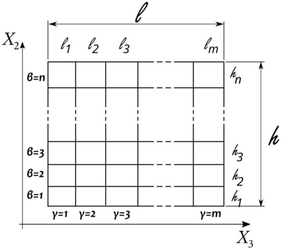
Figure 2.
The geometry of a doubly periodic GMC repeating unit cell subdivided into n × m rectangular subcells. The area of each subcell is lγ × hβ, where hγ and lβ are the height and length, respectively, of subcell γ, β. The total area of the RUC is .
Any subcell corresponds to a continuous material the constitutive law of which is given by
where , , and are the average stress, average total strain, average inelastic strain and average thermal strain tensors, respectively, of the material that fills the subcell; is the stiffness tensor. The average strains and stress of the complete RUCs are functions of the corresponding microscopic average values for each subcell and are defined as follows:
The relationships between microscopic and macroscopic strains are established by the imposition of the displacement and traction continuity conditions at the interfaces within the unit cell as well as at the interfaces between neighboring unit cells, in conjunction with the equilibrium conditions. Assuming the linear variation of displacements inside the subcell, the stress and strains are considered constant, and the average strains in the subcells are given in terms of the macroscopic strains in the form
where and are the appropriate concentration tensors and and are, respectively, the microscopic inelastic and thermal strains in all subcells. Thus, the resulting constitutive equation for infinitesimal strains is given by
In the case of elastic behavior, the effective constitutive equation of a composite is
The average stress and strain vectors are represented by the following:
The effective elastic stiffness tensor, , of the multiphase composite is given in closed form in terms of the elastic stiffness of the constituents:
The concentration tensor is estimated by the solution of a linear system with 6 × (m × n) algebraic equations for each RUC. An in-depth description of the method and the definition of constants can be found in [23,31]. The main advantage of the GMC is that in addition to its ability to homogenize the composite in order to create an effective constitutive equation, it also provides an approximation of the local stress and strain fields throughout the microstructure.
In the present application, GMC was interpreted to represent the response of carbon fiber-reinforced plastic (CFRP). The material system is composed of AS4 carbon fibers and high-strength epoxy resin 3501-6, which has a highly crosslinked structure that provides stiffness and strength but also reduces its ductility and leads to brittle behavior. The AS4/3501-6 material comes in the form of prepreg, which allows for the approximation of its microstructure as periodic. Stress and strain fields in such periodic configurations are investigated by a periodically repeating unit cell (RUC). Assuming for the AS4 fiber an elastic-only response and that the strong direction is aligned with longitudinal axis 1, the transversely isotropic elastic model was chosen as constitutive model. The model is described by the following equation:
where the components Cij from the stiffness matrix can be expressed in terms of five independent mechanical properties: longitudinal modulus of elasticity (E11), transverse modulus (E22), major Poisson ratio (v12), in-plane shear modulus (G12) and through-thickness Poisson’s ratio (v23). On the other hand, epoxy resin is considered homogeneous, elastic and isotropic, possessing the same mechanical properties in all directions. Thus, Equation (10) is simplified to
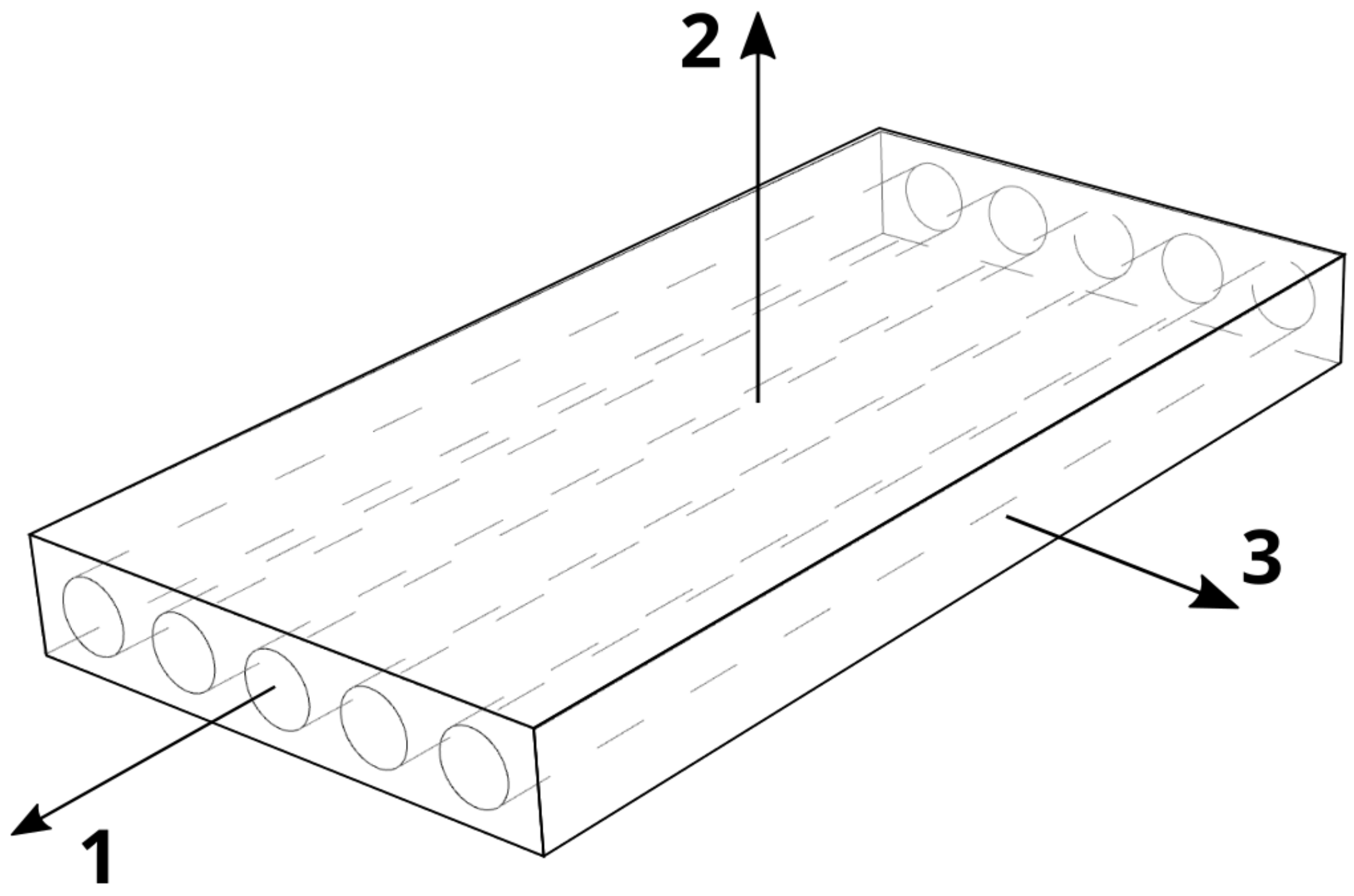
where only two independent mechanical properties are needed to express the Cij components: elastic modulus Em and Poisson’s ratio (v). A unidirectional (UD) lamina is used as the basic block in the laminate. We assume that the lamina thickness is very small compared with its other dimensions, that the bonding between fiber and matrix and between laminae are perfect, that lines perpendicular to the surface of the lamina remain straight and perpendicular to the surface after deformation and finally that the through-the-thickness stresses and strains are negligible (Figure 3).
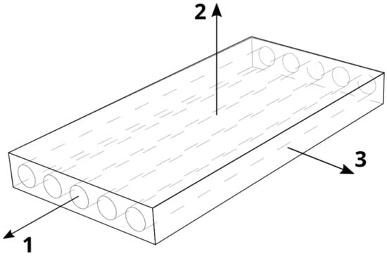
Figure 3.
A unidirectional lamina (UD) with a main coordination system 1,2,3 is fixed to the fiber direction (1), laminate (2) and thickness direction (3).
The accurate estimation of the effective properties of composite materials is at the heart of a micromechanical model, which requires the elastic properties of its constituents. Using the GMC method, we investigated the influence of various design parameters affecting the mechanical response of the composite by carrying out a series of parameter studies, where one parameter varied within a predefined range while the remaining were kept constant. For all studies, we assumed the use of the same constituents as reinforcement and matrix, carbon fiber AS4 and epoxy resin 3501-6, respectively. Additionally, we focused on small elastic mechanical responses; thus, we assumed a perfect bond between fiber and matrix. Taking into account the aforementioned assumptions, the parameters to be examined were limited to the fibers’ packaging and fiber volume fractions. For a constant, the nominal fiber volume fraction was set to Vf = 0.60, and seven different types of RUCs were chosen to investigate fiber packaging, categorized in two groups:
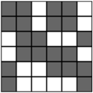
- Periodic fiber packaging RUCs depicted in Table 1, which can model RUCs with one or a maximum of two fibers. The characteristics are also the constraints related to the maximum allowable Vf. A major advantage of this type is the ability to approach the circular geometry of the fiber by discretizing the RUC in a large number of subcells.
 Table 1. Periodic fiber arrangements of doubly periodic RUC architectures applied with constant volume fraction Vf = 0.60.
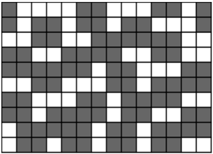
 - Random fiber packing arrangements, depicted in Table 2. These types can incorporate more than two fibers in one RUC in a random arrangement. Another characteristic of this RUC type is that it also allows for including fibers in close contact with others. Both types also allow for the control of RUC’s aspect ratio R:
Table 2. Random packing arrangements with constant fiber volume fraction Vf = 0.6.
For the parameter study of fiber volume fraction Vf, we chose two RUCs, REC.120 and RP.06 × 060 from Table 1 and Table 2, respectively. RP.06 × 06 as a random packaging RUC has to be defined manually, and therefore, we created 5 different sets of fiber packaging, each with a different fiber volume fraction (Table 3). Note that high volume fractions require increasing the number of fibers in the composite volume, which results in increases in the thinner matrix regions between fibers and in the contact between fibers as well.
Table 3.
Random packaging arrangements with various Vf.
2.2. Coupling GMC to CMA–ES Optimization Strategy
Nonisotropic materials like carbon fibers as well as polymeric materials like epoxy resins show variations in their experimentally measured mechanical properties, which in turn affects the effective properties of the composite materials. Therefore, more accurate effective properties can only be achieved by introducing in our model variations in the mechanical properties of the composite’s constituents. To solve the underlying complexity of the problem created by increases in problem parameters, we developed an optimization algorithm that couples the micromechanical model GMC with a general-purpose stochastic optimization algorithm, covariance matrix adaptation–evolution strategy (CMA–ES) [32]. The algorithm efficiently tunes the properties of all individual composites’ constituent properties along with their geometric arrangement in order to accurately predict the thermomechanical stress and deformation response of a previously experimentally tested composite material specimen [33]. CMA–ES has been successfully implemented [34,35], providing fast and efficient optimum results. During this procedure, a set of the selected parameters are tuned in an iterative process towards the minimization of the objective function. As CMA–ES randomly chooses each parameter value within a user-defined range, its bounds should be cautiously selected. Broad ranges might lead to unrealistic values, while narrow ranges might divert the algorithm from the global minimum. For the definition of the objective function, let be a parameterized class of micromechanics analytical models that simulate the composite material and will be used to estimate stress and strain responses under prescribed uniaxial loading. Consider to be the set of free material and geometric properties to be adjusted using the literature-derived experimental data, and let be the analytical predictions given the values of the parameter set . In this work, parameter estimation is based on response measurements of stress and strain pairs.
The difference between the experimental and the model-predicted response time histories takes the form
where is the analytical stress prediction and is the respective experimental stress value. Subscript corresponds to the total number of measured strain steps (number of observations). The uniaxial loading applied on the laminate structure is the same as the loading considered for the derivation of the experimental data.
In this work, a free distribution of the CMA–ES algorithm in C programming language is applied in parallel computing. The model-updating methodology evaluates the deviation between the experimental data and the predicted data of the analytical micromechanical model. As graphically presented in Figure 4, the process begins by sampling a set of material and geometrical parameter values from multivariate normal distributions with means and variances based on the ranges of the given bounds. Then, the GMC code is invoked to compute stress–strain responses interpolated to match the equivalent experimental measurements. The objective function is computed, and after the completion of a set of function evaluations (iterations), CMA–ES collects the minimum residuals for estimating new means and variances and commences a new iteration until the convergence criterion is met. In this work, convergence as the difference between the minimum values of two consecutive iterations was set to be less than . CMA–ES ends when convergence is fulfilled and the material and geometric parameters that correspond to the minimum best value correspond to the optimal parameters.
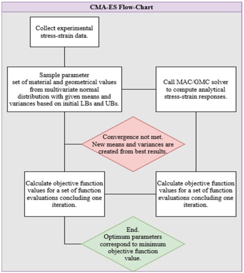
Figure 4.
A flow diagram of the applied CMA–ES model update method.
3. Experimental Data
All the experimental data used in our research to validate our model were obtained from various researchers mostly on cylindrical test specimens and collected from the Word Wide Failure exercise [33]. Testing on cylindrical specimens allows for the application of a wide range of biaxial and triaxial stresses that better reflect the real-life performance criteria of composite materials used in applications that impose multi-axial fields. Additionally, this method avoids problems associated with free edge effects that are encountered with coupons. Colvin et al. [36] investigated the mechanical responses along the longitudinal axes of cylindrical specimens subjected to axial loading, and Dichter et al. [37] studied the nonlinear stress–strain behavior of carbon fiber of reinforced plastic subjected to axial loads (Figure 5); the researchers reported that the stress–strain curve exhibited slight stiffening, with the modulus varying from E11,ini = 126 GPa at small strain to E11,sec = 142 GPa at failure. The investigation of transverse mechanical responses using both torsion and axial tension and the compression of thin-walled tubes revealed a linear stress–strain curve up to failure in the case of transverse tension [38]. The stress–strain curve for shear load was highly nonlinear, with failure in strong dependency from the test specimen. Alternatively, the shear strength can be estimated by the Iosipescu shear test to determine the in-plane shear modulus and strength of the unidirectional composite. In [39], the shear strength was estimated to be higher than the torsion.
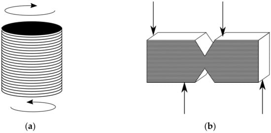
Figure 5.
(a) Torsion test and (b) Iosipescu test.
Fiber, matrix and lamina properties and strength parameters are listed in Table 4, and typical averaged stress–strain curves are shown in Figure 6. The mismatches in the longitudinal and transverse directions of the Young’s moduli of the two constituents are E11,fiber/E11, matrix ≈ 54 and E22,fiber/E22, matric ≈ 3.5, respectively. Because of the high property mismatch on the longitudinal axis, the effective Young’s modulus is mainly affected by the mechanical properties of the fibers. In contrast, due to the lower mismatch in the transverse direction, the contribution of the matrix is significant for the transverse effective properties.
Table 4.
The measured mechanical properties of constituents and the unidirectional lamina [33].
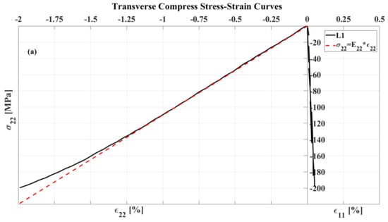
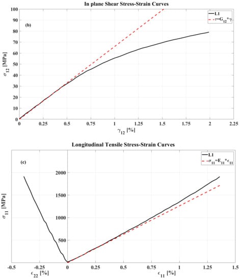
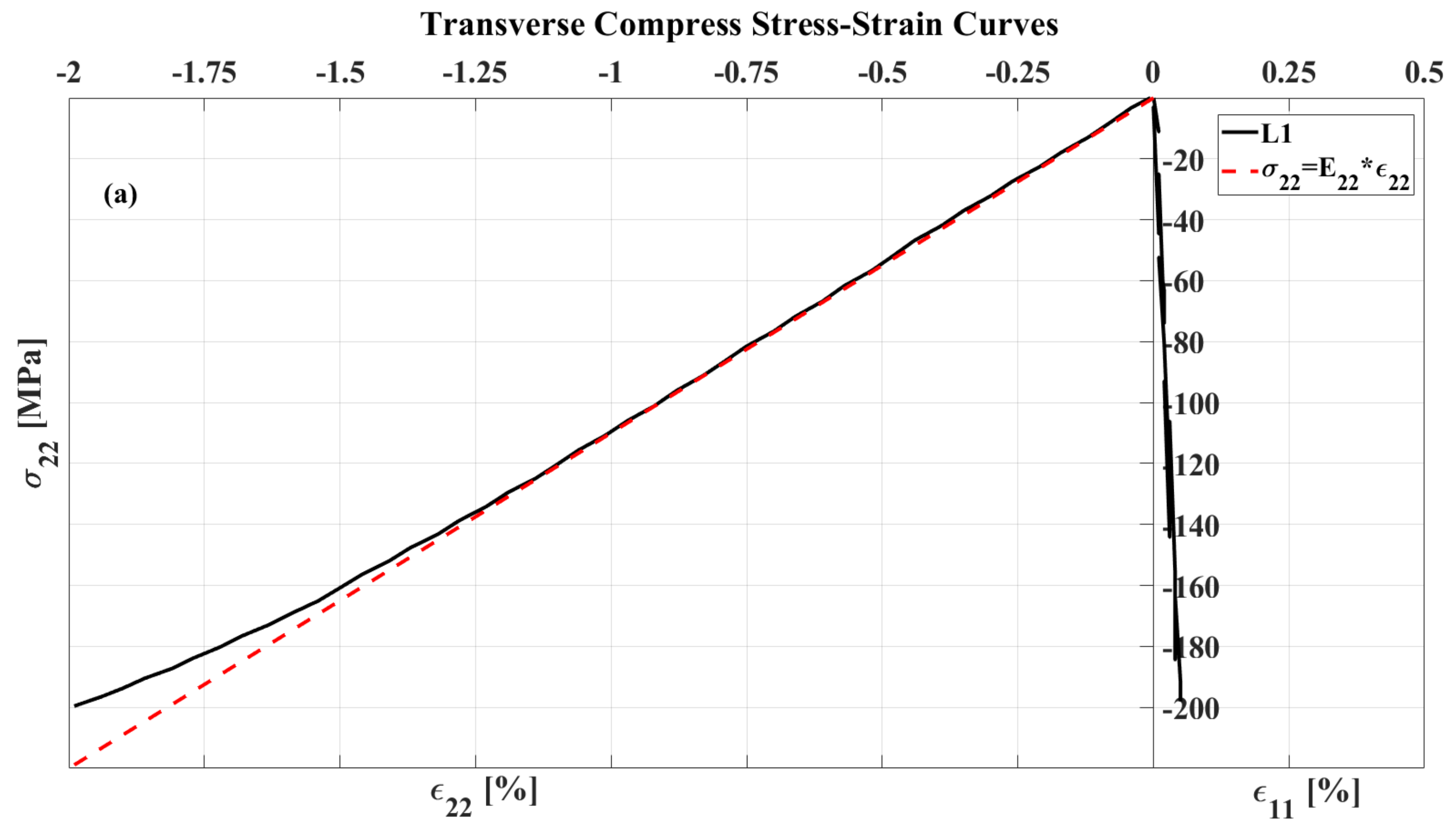
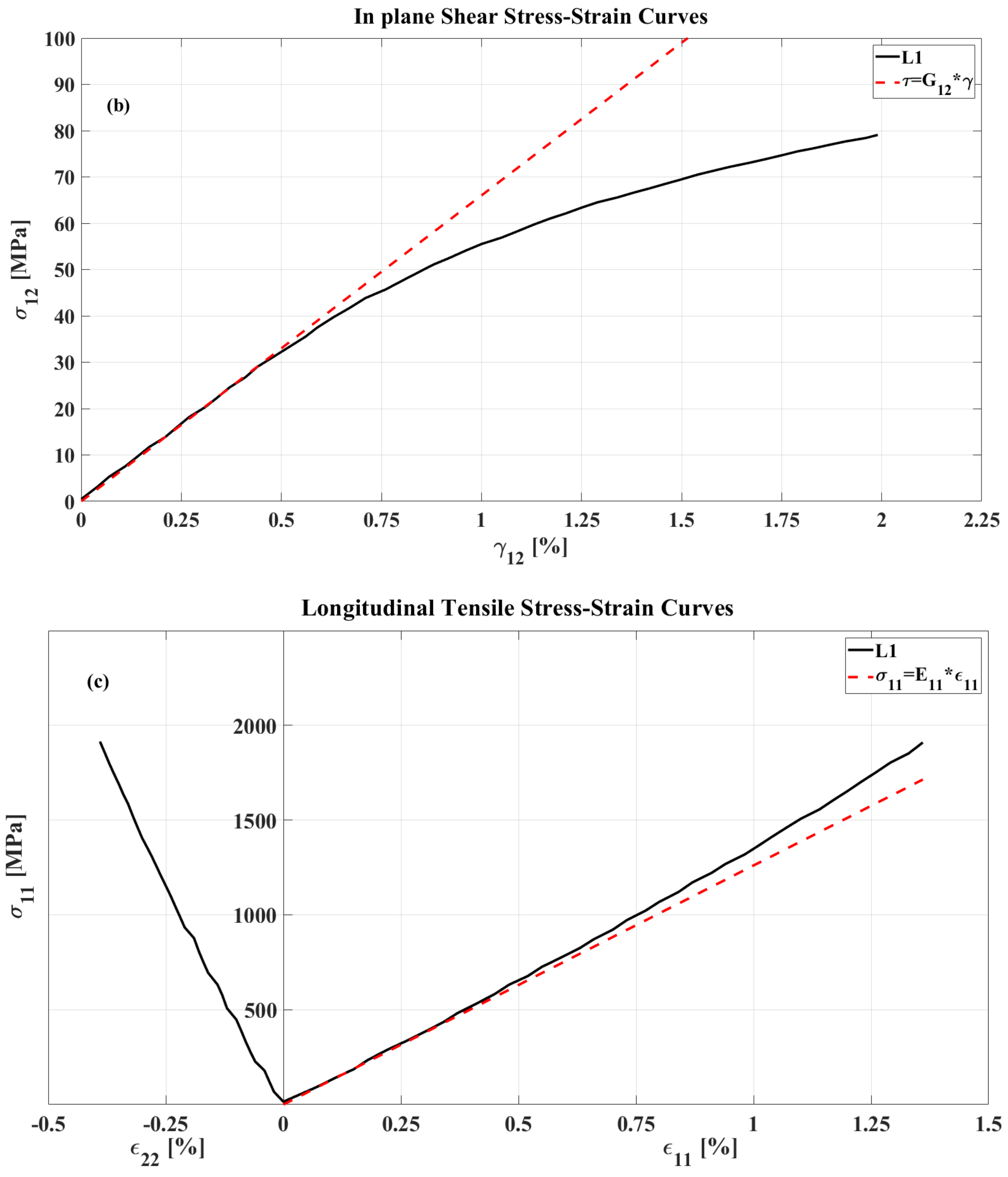
Figure 6.
Composite AS4/3501-6: (a) longitudinal tensile/compression test along 11 directions; no linear behavior on tensile; (b) transverse tensile/compressive stress along 22 directions; (c) plane shear test on plane 12. Linear behavior is indicated by γ12 < 0.5%, whereas γ12 > 0.5% composite indicates nonlinear behavior.
The stress–strain curves in Figure 6 indicate two stages in the mechanical response of the cylindrical composite material, a linear and a nonlinear deformation. Linear elastic deformation is limited to strain values below 0.5% in the case of longitudinal tension and in-plane shear, whereas in the case of transverse compression, we notice linear elastic behavior for strains up to approximately 1.0%. Above the aforementioned limits, the composite starts to behave nonlinearly but with differences in the slopes. In both transverse compression and plane shear, the stress–strain curve attains a negative slope, an indication of the softening of the material. On the other hand, for linear tension, the stress–strain curve shows a slight upward concave, which implies a stiffening of the material.
4. Results and Discussion
4.1. Effective Properties: Influence of Fiber Architecture
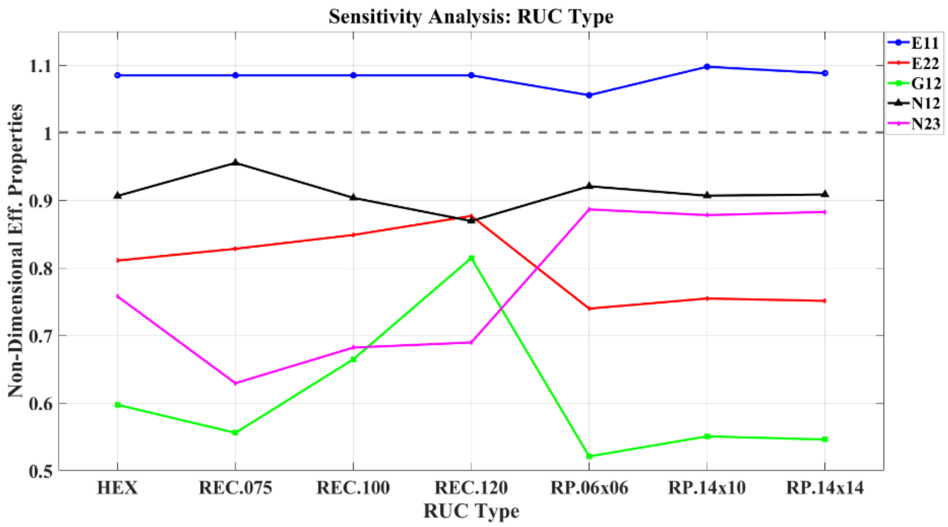
The predicted results for the effective properties in the case of constant fiber volume fraction Vf = 0.6 are presented in Table 5, Table 6 and Table 7. The predicted values in each table are compared with the measured values, and for each model, the percentage deviation between the predicted and measured effective properties is derived. Figure 7 illustrates the influence of packing arrangement on the predicted effective properties. For the ease of comparison, we used nondimensional values of the predicted effective properties by normalizing them with the respective experimentally measured values. We notice that the predicted values of longitudinal elastic modulus E11 are almost constant independent of the type of RUC, as expected. On the other hand, the predicted in-plane shear modulus G12 shows the largest deviation from the measured values and a strong dependency from the RUC’s aspect ratio in the case of RECTANGLE RUC. Changing the aspect ratio for the constant fiber volume fraction leads to an increase in the matrix mass between fibers, which in turn causes a corresponding increase in the shear modulus. Clearly, the stiffest transversal response (E22) is associated with the REC120 RUC, followed by REC100, R075, and HEX, with all random being the softest. This is clearly related to the relative matrix volume along the loading direction and the small mismatch in mechanical properties between the two constituents. It is also noticeable that in the case of randomly packed RUCs, the influence of the aspect ratio or the total number of subcells is small on all the effective properties. In this case, the largest deviations are observed in the case of transverse elastic modulus E22 and in-plane shear modulus G12. These results clearly indicate that packing geometry significantly influences the transverse response and that this influence increases with the increase in the reciprocal aspect ratio. These trends are consistent with those discussed in the literature [40,41,42]. Rectangle REC120 with a length-to-height ratio equal to 1.20 provides the most accurate estimations of the effective properties except for Poisson’s ratio v23.
Table 5.
Comparisons between the measured experimental (EXP) and the predicted effective properties for HEXAGONAL and RECTANGLE with R = 1.0 (square) RUCs.
Table 6.
Comparisons between the measured experimental (EXP) and the predicted effective properties for RECTANGLE RUCs at various aspect ratios.
Table 7.
Comparisons between the measured experimental (EXP) and the predicted effective properties for RANDOM PACKAGING ARRANGEMENTS for various aspect ratios and subcell numbers.
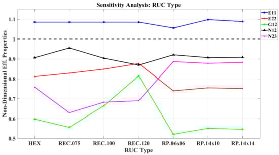
Figure 7.
Nondimensional predicted effective properties for various RUCs. A value of 1 corresponds to measured experimental data.
4.2. Effective Properties: Influence of Volume fraction
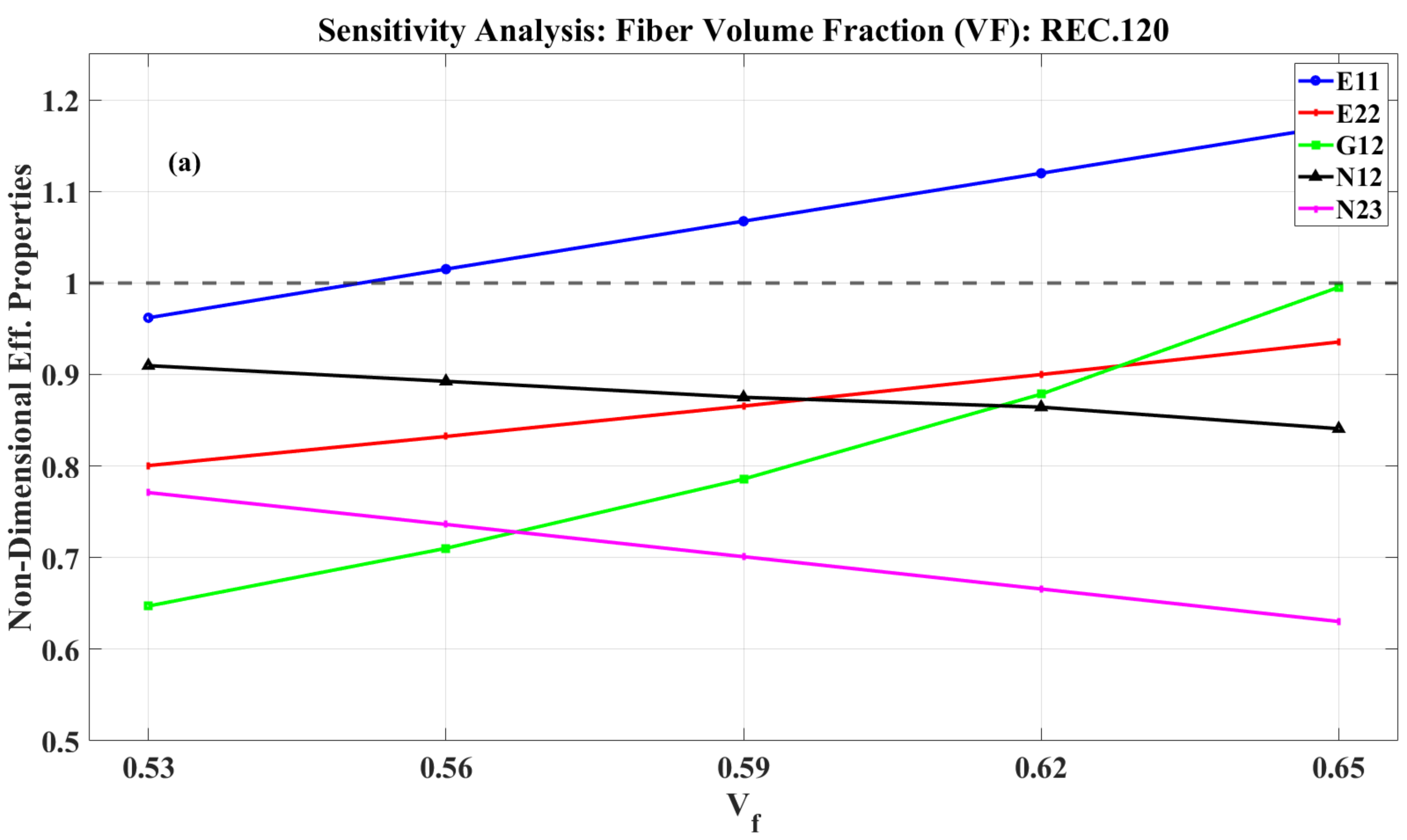
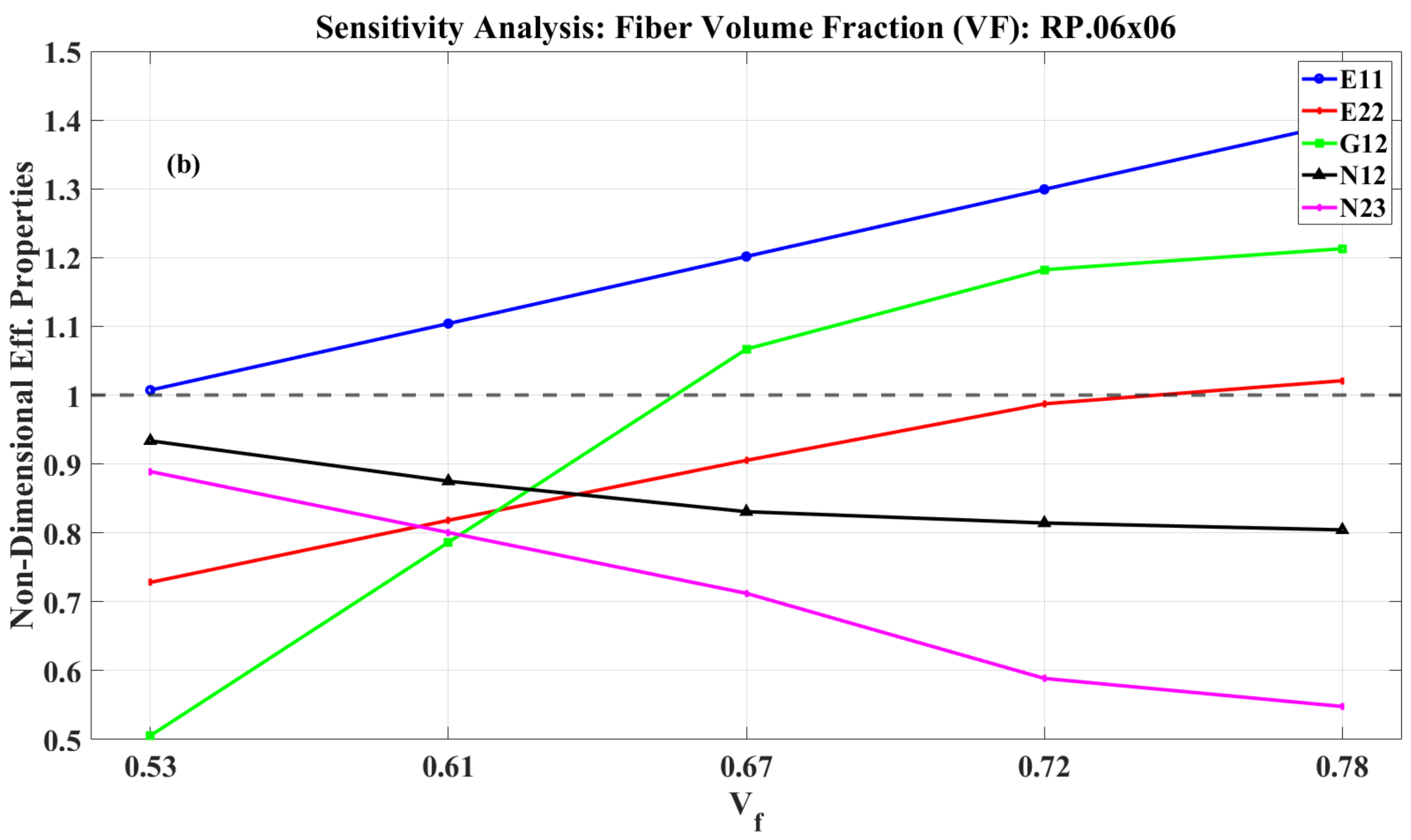
The predicted results for the effective properties in the case of influence volume fractions are presented in Table 8 and Table 9. The curves of the nondimensional effective properties vs. the volume fractions in Figure 8 reveal a proportional relationship with the exception of Poisson’s ratios. Qualitatively, the model results are very similar to the results presented by Aboudi regarding the effective property predictions of a glass/epoxy composite as a function of fiber volume fraction Vf for three different RUCs.
Table 8.
Comparisons between the measured experimental (EXP) and the predicted effective properties for RANDOM PACKAGING ARRANGEMENT RP.06 × 06 with different fiber volume fraction ratios.
Table 9.
Comparisons between the measured experimental (EXP) and the predicted effective properties for PERIODIC PACKAGING ARRANGEMENT REC.120 with different fiber volume fraction ratios.
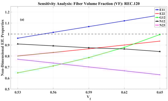
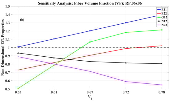
Figure 8.
Nondimensional predicted effective properties as a function of fiber volume fraction Vf. (a) Periodic fiber packaging using REC.120 as a RUC. (b) Random fiber packaging using RP.06 × 0.6 as a RUC.
Both longitudinal and transverse stiffnesses (E11, E22) indicate an almost linear dependence on the fiber volume fraction independent of the RUC type. At fiber volume fractions between 0.56 and 0.67, we observe similar results for longitudinal stiffness, ranging between 1.0 and 1.2. On the other hand, for the transverse stiffness, we note an underprediction for random fiber packaging RUCs with values lower than those of REC.120. This can be attributed to the existence of contact between fibers in RP.06×06. In the case of G12, we notice significant differences in dependence on Vf between the two RUCs. For REC.120, G12 constantly increases, whereas for RP.06×06, it shows a tendency to converge to a constant value in higher fiber volume fractions. Both Poisson’s ratios, in contrast, imply inversely proportional behavior in relation to the changes in Vf.
4.3. Influence of Constituents Mechanical Properties
The analytical GMC model code is herein introduced in its parameterized scheme in order to facilitate the optimization algorithm. The parameterized analytical model passed to the CMA–ES consisted of nine design parameters in total. The first seven design parameters pertain to the material properties of fiber and matrix. Specifically, there are five fiber material parameters that represent the longitudinal modulus , transverse modulus , Poisson ratios and and shear modulus . There are two matrix material parameters that represent the modulus of elasticity and the Poisson ratio . Finally, two more design parameters have been included in order to account for the geometric arrangement of the laminate analytical model, representing the fiber volume fraction and the aspect ratio of the RUC . The nominal material parameters for the fiber were , , , and and for the matrix, they were and . Similarly, the geometric parameters had nominal values of and . All analyses were performed using the same RUC architecture ID number , which had proved the most efficient from the precedent sensitivity analyses.
The CMA–ES framework was implemented at a range of ±15% from the nominal values for the design parameter bounds. The optimization process converged after 155 iterations performing 100 function evaluations per iteration at several seconds per run. Thus, the total number of runs was approximately 15,500 completed in approximately 3 h, owing to the highly parallelizable potential of the applied CMA–ES algorithm.
Table 10 summarizes the results of the previously described updating process. The lower (LB) and upper (UB) bounds along with the nominal means are also presented. Specifically, the first column presents the number of design parameters; the second column presents each parameter used; the third, fourth and fifth columns present the lower bound, mean and upper bound, respectively; and the last column presents the updated material and geometry parameters according to the described parameterization.
Table 10.
The updated design variable parameters and design bounds (LB and UB) of the examined micromechanics model.
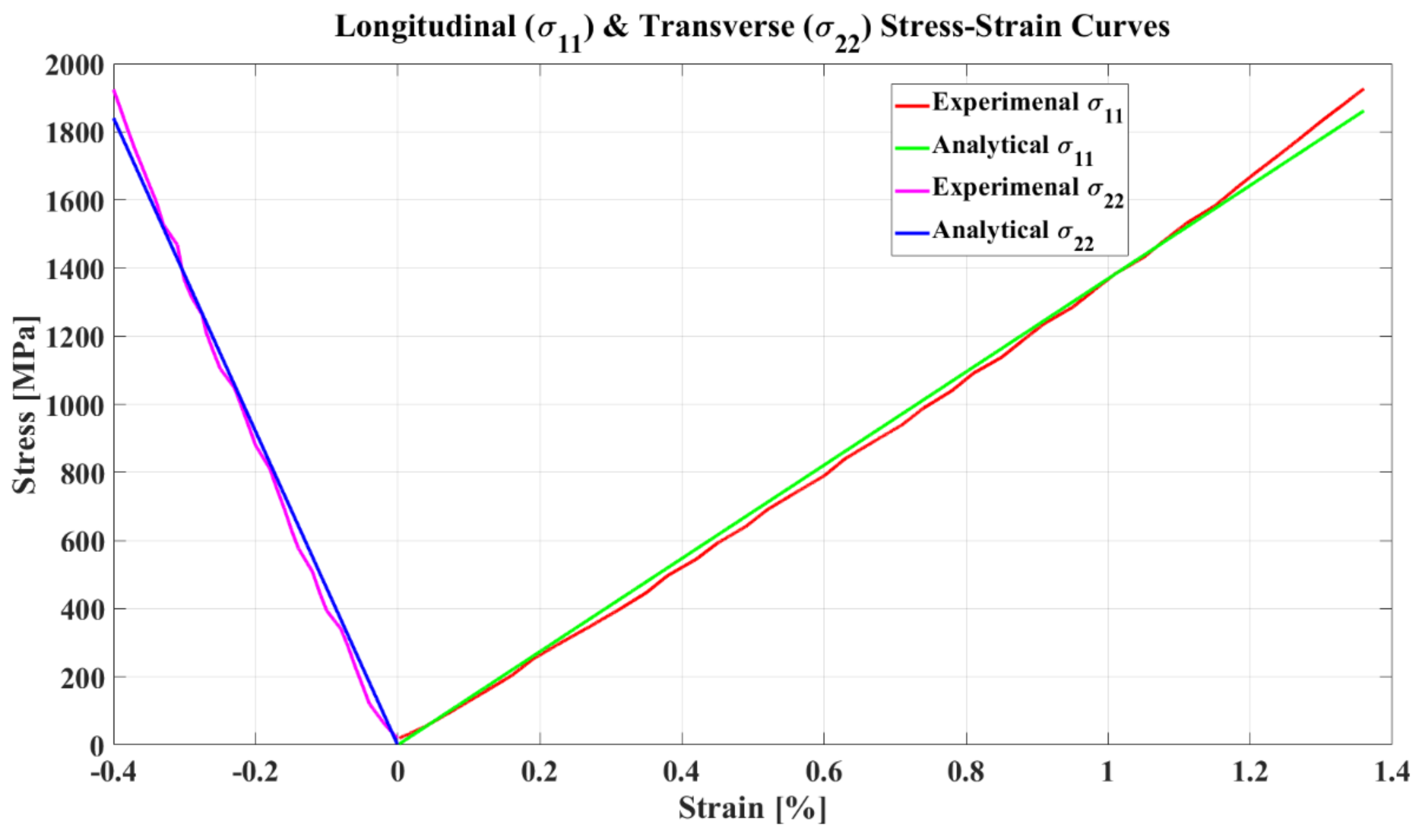
After the CMA–ES algorithm converged, the produced optimal parameters were used in the analytical micromechanics model in order to evaluate the longitudinal and transverse stress–strain curves. These analytical stress–strain curves are graphically compared with the experimental ones. Figure 9 presents the comparison between the measured experimental stress–strain curves and the analytically predicted respective ones of the updated micromechanics model. The red continuous line represents the experimentally measured longitudinal stress–strain curve; the green continuous line presents the respective predicted analytical one; and the magenta continuous line represents the experimentally measured transverse stress–strain curve compared with the blue continuous line presenting the respective analytical one.
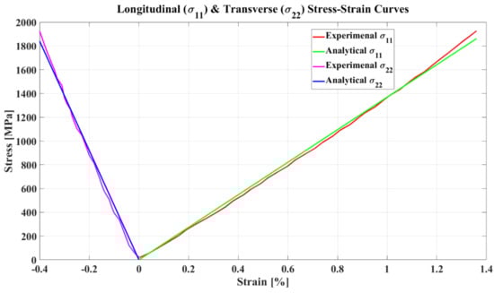
Figure 9.
Comparisons between the experimentally measured and analytically predicted by optimal model of longitudinal and transverse stress–strain curves for uniaxial loading.
The presented result proves a nearly perfect match between the experimental data and the analytically predicted longitudinal and transverse stress–strain curves across the whole range of strain values. The nearly perfect match is numerically quantified in the overall minimum value computed by Equation (13), 9.10 × 10⁻⁴, which is visually confirmed by Figure 9. A small deviation can be noticed, attributed to the low accuracy of the derived experimental values, where only a few decimals were available. The above result increases the confidence of a high-fidelity analytical micromechanics model and provides strong evidence of the efficiency of the proposed GMC–CMA–ES optimization scheme.
Furthermore, Table 11 presents the effective mechanical properties of the laminate. The difference in the stiffness along fiber is 8.65%. This is a reasonable result that lies within the uncertainty threshold given the experimental test and the nature of such a physical value. The highest differences are observed at and , 16.83% and 40.70%, respectively. This is an obvious result, keeping in mind that such material parameters cannot be practically measured through the experimental process but are only computed indirectly. At last, the Poisson values and are also derived indirectly during the experiment, and the observed discrepancies cannot be practically addressed.
Table 11.
Comparisons between the experimental and model updated laminate mechanical properties.
The ε predicted results constitute the tuned parameters derived by the CMA–ES algorithm, aiming to minimize the discrepancies between the experimental stress data and the equivalent GMC analytically computed data. Thus, CMA–ES is used to reconcile discrepancies and achieve a high-fidelity analytical model that can confidently reflect the experimental measurements. The whole process does not aim to optimize the design of a structure but only to tune an analytical model using experimental information.
5. Conclusions
The current work has explored a new material design methodology based on a combination of a GMC micromechanical model and a state-of-the-art covariance matrix adaptation (CMA–ES) optimization algorithm [32,34,35]. The methodology was validated by comparing the predicted effective properties with the measured experimental data presented in the work of Hinton et al. [33].
To this end, a two-step approach was developed. Initially, a parameter analysis of the influence of fiber packaging arrangement and volume fraction on the predicted effective properties was implemented. In the case of the fiber packaging arrangement, we noticed that the longitudinal stiffness was independent of the RUC type as expected. On the other hand, in both transverse stiffness and in-plane shear modulus, we observed a linear dependence on the RUC aspect ratio. Since the fiber volume fraction was considered constant, the only parameter left for fine tuning the mechanical properties was the RUC aspect ratio, which allows for changes in matrix volume on a predefined direction. For the random fiber arrangement, the predicted effective properties were almost constant without any effect from either the number of subcells or the aspect ratio R. Next, we studied the influence of the fiber volume fraction by again assuming periodic and random fiber arrangements. As expected, both longitudinal and transverse stiffness showed linear dependence on the fiber volume fraction, with similar prediction in the case of longitudinal stiffness. Distinctive differences between the two fiber arrangements were observed in the in-plane shear modulus. For the periodic fiber arrangement (RUC.120), G12 shows a positive curve. On the other hand, for random fiber arrangement (RP.06 × 06), G12 has a negative curve, which indicates a tendency to converge to a constant value.
Author Contributions
Conceptualization, D.G. and I.Z.; methodology, I.Z, D.G. and A.A.; software, A.A. and I.Z.; validation, I.Z., A.A. and D.G.; formal analysis, I.Z. and D.G.; investigation, I.Z.; resources, I.Z. and A.A.; data curation, I.Z. and A.A.; writing—original draft preparation, I.Z. and A.A.; writing—review and editing, I.Z. and D.G.; visualization, I.Z., A.A. and D.G.; supervision, D.G.; project administration, D.G.; funding acquisition, D.G. All authors have read and agreed to the published version of the manuscript.
Funding
This research has been co-financed by the European Regional Development Fund of the European Union and Greek National Funds through Operational Program Competitiveness, Entrepreneurship, and Innovation, under the call RESEARCH—CREATE—INNOVATE (project code: T1EDK:05393).
Institutional Review Board Statement
Not applicable.
Informed Consent Statement
Not applicable.
Data Availability Statement
Not applicable.
Conflicts of Interest
The authors declare no conflict of interest.
References
- Voigt, W. Lehrbuch der Kristallphysik; Vieweg+Teubner Verlag: Wiesbaden, Germany, 1966. [Google Scholar] [CrossRef]
- Reuss, A. Berechnung der Fließgrenze von Mischkristallen auf Grund der Plastizitätsbedingung für Einkristalle. Z. Angew. Math. Mech. 1929, 9, 49–58. [Google Scholar] [CrossRef]
- Hill, R. The Elastic Behaviour of a Crystalline Aggregate. Proc. Phys. Soc. Sect. A 1952, 65, 349. [Google Scholar] [CrossRef]
- Bohm, H.J. A Short Introduction to Basic Aspects of Continuum Micromechanics; ILSB-Arbeitsbericht 206; Vienna University of Technology: Vienna, Austria, 2010. [Google Scholar]
- Eshelby, J.D. The determination of the elastic field of an ellipsoidal inclusion, and related problems. Proc. R. Soc. Lond. Ser. A Math. Phys. Sci. 1957, 241, 376–396. [Google Scholar] [CrossRef]
- Mori, T.; Tanaka, K. Average stress in matrix and average elastic energy of materials with misfitting inclusions. Acta Met. 1973, 21, 571–574. [Google Scholar] [CrossRef]
- Pan, J.; Bian, L. A re-formulation of the Mori–Tanaka method for predicting material properties of fiber-reinforced polymers/composites. Colloid Polym. Sci. 2019, 297, 529–543. [Google Scholar] [CrossRef]
- Barral, M.; Chatzigeorgiou, G.; Meraghni, F.; Léon, R. Homogenization using modified Mori-Tanaka and TFA framework for elastoplastic-viscoelastic-viscoplastic composites: Theory and numerical validation. Int. J. Plast. 2020, 127, 102632. [Google Scholar] [CrossRef] [Green Version]
- Mercier, S.; Molinari, A.; Berbenni, S.; Berveiller, M. Comparison of different homogenization approaches for elastic–viscoplastic materials. Model. Simul. Mater. Sci. Eng. 2012, 20, 024004. [Google Scholar] [CrossRef]
- Desrumaux, F.; Meraghni, F.; Benzeggagh, M.L. Generalised Mori-Tanaka Scheme to Model Anisotropic Damage Using Numerical Eshelby Tensor. J. Compos. Mater. 2001, 35, 603–624. [Google Scholar] [CrossRef]
- Charalambakis, N.; Chatzigeorgiou, G.; Chemisky, Y.; Meraghni, F. Mathematical homogenization of inelastic dissipative materials: A survey and recent progress. Contin. Mech. Thermodyn. 2018, 30, 1–51. [Google Scholar] [CrossRef] [Green Version]
- Benveniste, Y. Revisiting the generalized self-consistent scheme in composites: Clarification of some aspects and a new formulation. J. Mech. Phys. Solids 2008, 56, 2984–3002. [Google Scholar] [CrossRef]
- Hashin, Z. Thermoelastic properties of fiber composites with imperfect interface. Mech. Mater. 1990, 8, 333–348. [Google Scholar] [CrossRef]
- Hervé-Luanco, E.; Joannès, S. Multiscale modelling of transport phenomena for materials with n-layered embedded fibres. Part I: Analytical and numerical-based approaches. Int. J. Solids Struct. 2016, 97–98, 625–636. [Google Scholar] [CrossRef]
- Benveniste, Y.; Milton, G. The effective medium and the average field approximations vis-à-vis the Hashin–Shtrikman bounds. II. The generalized self-consistent scheme in matrix-based composites. J. Mech. Phys. Solids 2010, 58, 1039–1056. [Google Scholar] [CrossRef]
- Christensen, R.; Lo, K. Solutions for effective shear properties in three phase sphere and cylinder models. J. Mech. Phys. Solids 1979, 27, 315–330. [Google Scholar] [CrossRef]
- Sekkate, Z.; Aboutajeddine, A.; Seddouki, A. Elastoplastic mean-field homogenization: Recent advances review. Mech. Adv. Mater. Struct. 2022, 29, 449–474. [Google Scholar] [CrossRef]
- Ortolano, J.M.; Hernandez, J.A.; Oliver, J.A. A Comparative Study on Homogenization Strategies for Multi-Scale Analysis of Materials; Monograph CIMNE: Barcelona, Spain, 2013; Volume 135. [Google Scholar]
- Aboudi, J. Micromechanical Analysis of Composites by the Method of Cells. Appl. Mech. Rev. 1989, 42, 193–221. [Google Scholar] [CrossRef]
- Wang, J.; Andreasen, J.; Karihaloo, B. The solution of an inhomogeneity in a finite plane region and its application to composite materials. Compos. Sci. Technol. 2000, 60, 75–82. [Google Scholar] [CrossRef]
- Sangani, A.S.; Lu, W. Elastic coefficients of composites containing spherical inclusions in a periodic array. J. Mech. Phys. Solids 1987, 35, 1–21. [Google Scholar] [CrossRef]
- Cohen, I. Simple algebraic approximations for the effective elastic moduli of cubic arrays of spheres. J. Mech. Phys. Solids 2004, 52, 2167–2183. [Google Scholar] [CrossRef]
- Paley, M.; Aboudi, J. Micromechanical analysis of composites by the generalized cells model. Mech. Mater. 1992, 14, 127–139. [Google Scholar] [CrossRef]
- Aboudi, J. Micromechanical Analysis of Composites by the Method of Cells—Update. Appl. Mech. Rev. 1996, 49, S83–S91. [Google Scholar] [CrossRef]
- Fish, J. Multiscale Methods; Oxford University Press: Oxford, UK, 2009. [Google Scholar] [CrossRef]
- Kanouté, P.; Boso, D.P.; Chaboche, J.L.; Schrefler, B.A. Multiscale Methods for Composites: A Review. Arch. Comput. Methods Eng. 2009, 16, 31–75. [Google Scholar] [CrossRef]
- Feyel, F.; Chaboche, J.-L. FE2 multiscale approach for modelling the elastoviscoplastic behaviour of long fibre SiC/Ti composite materials. Comput. Methods Appl. Mech. Eng. 2000, 183, 309–330. [Google Scholar] [CrossRef]
- Pan, L.; Adams, D.O.; Rizzo, F.J. Boundary element analysis for composite materials and a library of Green’s functions. Comput. Struct. 1998, 66, 685–693. [Google Scholar] [CrossRef]
- Liu, Y.; Nishimura, N.; Otani, Y.; Takahashi, T.; Chen, X.L.; Munakata, H. A Fast Boundary Element Method for the Analysis of Fiber-Reinforced Composites Based on a Rigid-Inclusion Model. J. Appl. Mech. 2005, 72, 115–128. [Google Scholar] [CrossRef]
- Pindera, M.-J.; Bednarcyk, B.A. An efficient implementation of the generalized method of cells for unidirectional, multi-phased composites with complex microstructures. Compos. Part B Eng. 1999, 30, 87–105. [Google Scholar] [CrossRef]
- Aboudi, J. The Generalized Method of Cells and High-Fidelity Generalized Method of Cells Micromechanical Models—A Review. Mech. Adv. Mater. Struct. 2004, 11, 329–366. [Google Scholar] [CrossRef]
- Hansen, N. The CMA Evolution Strategy: A Comparing Review. In Towards a New Evolutionary Computation; Springer: Berlin/Heidelberg, Germany, 2007; pp. 75–102. [Google Scholar] [CrossRef]
- Hinton, M.J.; Kaddour, A.S.; Soden, P.D. Failure Criteria in Fibre-Reinforced-Polymer Composites; Elsevier: Amsterdam, The Netherlands, 2004. [Google Scholar] [CrossRef]
- Giagopoulos, D.; Arailopoulos, A. Computational framework for model updating of large scale linear and nonlinear finite element models using state of the art evolution strategy. Comput. Struct. 2017, 192, 210–232. [Google Scholar] [CrossRef]
- Zacharakis, I.; Giagopoulos, D.; Arailopoulos, A.; Markogiannaki, O. Optimal finite element modeling of filament wound CFRP tubes. Eng. Struct. 2022, 253, 113808. [Google Scholar] [CrossRef]
- Colvin, G.E.; Swanson, S.R. In-Situ Compressive Strength of Carbon/Epoxy AS4/3501-6 Laminates. J. Eng. Mater. Technol. 1993, 115, 122–128. [Google Scholar] [CrossRef]
- Ditcher, A.K.; Rhodes, F.E.; Webber, J.P.H. Non-linear stress-strain behaviour of carbon fibre reinforced plastic laminates. J. Strain Anal. Eng. Des. 1981, 16, 43–51. [Google Scholar] [CrossRef]
- Swanson, S.R.; Toombes, G.R. Characterization of Prepreg Tow Carbon/Epoxy Laminates. J. Eng. Mater. Technol. 1989, 111, 150–153. [Google Scholar] [CrossRef]
- Swanson, S.; Messick, M.; Toombes, G. Comparison of torsion tube and Iosipescu in-plane shear test results for a carbon fibre-reinforced epoxy composite. Composites 1985, 16, 220–224. [Google Scholar] [CrossRef]
- Böhm, H.; Rammerstorfer, F.; Weissenbek, E. Some simple models for micromechanical investigations of fiber arrangement effects in MMCs. Comput. Mater. Sci. 1993, 1, 177–194. [Google Scholar] [CrossRef]
- Mueller, A. A finite element method for microstructural analysis. Compos. Eng. 1994, 4, 361–376. [Google Scholar] [CrossRef]
- Nakamura, T.; Suresh, S. Effects of thermal residual stresses and fiber packing on deformation of metal-matrix composites. Acta Met. Mater. 1993, 41, 1665–1681. [Google Scholar] [CrossRef]


Publisher’s Note: MDPI stays neutral with regard to jurisdictional claims in published maps and institutional affiliations. |
© 2022 by the authors. Licensee MDPI, Basel, Switzerland. This article is an open access article distributed under the terms and conditions of the Creative Commons Attribution (CC BY) license (https://creativecommons.org/licenses/by/4.0/).