“Time”-Covariant Schrödinger Equation and the Canonical Quantization of the Reissner–Nordström Black Hole

Abstract

A “time”-covariant Schrödinger equation is defined for the minisuperspace model of the Reissner–Nordström (RN) black hole, as a “hybrid” between the “intrinsic time” Schrödinger and Wheeler–DeWitt (WDW) equations. To do so, a reduced, regular, and “time(r)”-dependent Hamiltonian density was constructed, without “breaking” the re-parametrization covariance $r\to f(\tilde{r})$. As a result, the evolution of states with respect to the parameter r and the probabilistic interpretation of the resulting quantum description is possible, while quantum schemes for different gauge choices are equivalent by construction. The solutions are found for Dirac’s delta and Gaussian initial states. A geometrical interpretation of the wavefunctions is presented via Bohm analysis. Alongside this, a criterion is presented to adjudicate which, between two singular spacetimes, is “more” or “less” singular. Two ways to adjudicate the existence of singularities are compared (vanishing of the probability density at the classical singularity and semi-classical spacetime singularity). Finally, an equivalence of the reduced equations with those of a 3D electromagnetic pp-wave spacetime is revealed.

1. Introduction

The quantization of gravity possesses a fundamental place in the realm of theoretical physics. As was argued by Claus Kiefer [1], there are mainly three arguments that motivate such a quest: the first motivation is based more on philosophical reasons and the idea that all fundamental interactions should be unified at some energy scale. Hence, if a coherent quantum theory exists that describes those fundamental interactions, gravity should be included as well. The second motivation is related to the appearance of singularities in the classical theory of gravity, at is described by general relativity. The hope is that a quantum theory of gravity will be free of such pathological situations. Finally, the third motivation is related to the so-called “problem of time” as can be found in [2,3,4,5,6,7]. The main reason that such a problem arises is that in the conventional quantum theory, time is an external parameter, while in the general theory of relativity, there is no preferred or fundamental notion of time. This is due to the diffeomorphism invariance of the theory. Furthermore, this invariance results in a singular Lagrangian and Hamiltonian density respectively, which implies constraint equations in addition to the dynamics. The relation between constraint equations and diffeomorphisms can be found in [8], as well as in [9].

The appearance of constraints results in two main approaches in the quantization procedure: the first is to solve the constraints before quantization, while the second is to impose the constraints at the quantum level, as restrictions upon the states. One of the main paths to deal with the above approaches is the so-called “canonical quantization”, where the canonical variables that describe the gravitational field are promoted to operators and the Poisson brackets are replaced by operator commutators. Some of the original work in the direction of the Hamiltonian formalism of gravity was given in [10,11,12,13,14,15,16,17,18,19].

Related to the second procedure, the most famous result is the Wheeler–DeWitt equation [20,21,22,23,24,25], which results from the quadratic constraint, or in other words, from the variation of the gravitational action with respect to the lapse function, in the canonical formalism. This equation contains no external parameter in which the term “time” could be assigned. In fact, due to its hyperbolic nature, the “time” parameter is encoded in the degrees of freedom that appear, hence the name “intrinsic” time. Thus, additional hypothesis are needed in order to define a “time” and hence arrive at some sort of a Schrödinger equation. One of the problems arising due to the hyperbolic nature is the difficulty in defining a proper Hilbert space as in the conventional quantum theory.

When it comes to the first procedure, the usual approach is to introduce quantities ${\chi }^A$, which will be functions of the degrees of freedom and impose a suitable gauge choice. To this end, a “true” Hamiltonian density $h_A$ can be constructed, which depends only on the true gravitational degrees of freedom. The constraint equation has the form:

$$\begin{array}{c}{P}_A+h_A=0,\hfill \end{array}$$

(1)

where $P_A$ are the conjugate momenta of the introduced quantities ${\chi }^A$. A Schrödinger-type equation can then be realized from the above equation, with the identification $P_A=ih\frac{\delta }{\delta {\chi }^A}$:

$$\begin{array}{c}ih\frac{\delta \mathsf{\Psi }}{\delta {\chi }^A}={\widehat{h}}_A\mathsf{\Psi }.\hfill \end{array}$$

(2)

An extensive analysis of this approach can be found in [5,26,27]. Now, since in the constraint, the momenta appear quadratically, in many cases, it is very difficult to obtain a closed form density $h_A$. This is one of the reasons that many authors have assumed the existence of matter in order to define a standard of time [28,29,30,31]. In this case, a Hilbert space can be defined, and alongside this, a probabilistic interpretation could be provided [5]. As was argued by Barvinsky [6], choosing a gauge breaks the gauge invariance of the theory and, hence, for each different gauge (classically equivalent systems), one has different quantum theories, which must be proven to be equivalent. Another problem is that the Hamiltonian density $h_A$ is the square root of the true degrees of freedom and the “time” variables, which implies that in many cases, it will remain real only for a specific domain of the “time” variable. Furthermore, since it is a square root operator, it is known that it can be handled only if the quantity whose root is being taken is self-adjoint and positive [5]. Note also that ${\widehat{h}}_A$ are “time” dependent, which implies that we cannot reproduce the Wheeler–DeWitt equation from (2). This is not something to worry about; it simply reveals the different quantization approaches. An interesting new approach to the problem of time can be found in [32].

These interesting questions are very difficult to tackle in the full theory of gravity. In order to acquire some insight, people have worked on simplified models such as minisuperspace Lagrangians, where the isometries of spacetime are enough, in order to render the system from infinite to finite dimensional. In cosmology, such examples are the FLRW geometries, the Bianchi types, and the Kantowski–Sachs metric [33]. Additionally, there are the point-like sources such as Schwarzschild (S) [34] and Reissner–Nordström (RN) [35] spacetimes. For instance, in [36], the author argued that the classical properties of an intrinsic time variable, as the scale factor in FLRW geometry, would emerge in some sense, through the interaction with fermionic degrees of freedom. The semiclassical quantum cosmology was investigated [37] for the FLRW minisuperspace model with electromagnetic field perturbations around the background. Wave packets were constructed for the coupling of gravity and a massless, as well as a massive scalar field in the FLRW geometry [38]. Another work with the same underlying geometry and in the presence of scalar field can be found here [39]. For the case of general, spatial cosmologies in the presence of a scalar field, exact solutions have been found [40]. In the case that the Hamilton–Jacobi equation is separable for the cosmological models under consideration, it has been proven [41] that these models can be quantized as ordinary gauge systems. The solutions to the Wheeler–DeWitt equation for the Reissner–Nordström–de Sitter black hole were interpreted via the de Broglie–Bohm theory [42]. The use of conditional symmetries was employed for the quantum description of the general Bianchi Type I, with and without the presence of a cosmological constant [43]. In the same line of thought, the canonical quantization of the Reissner–Nordström black hole can be found in [44], where the interpretation of the solutions to the Wheeler–DeWitt (WDW) equation is based on the semiclassical corrected geometry via Bohm’s analysis. Another work that shares some common ground with what we intend to do in this paper is [45]. The authors managed to decouple the reparametrization invariance for some minisuperspace models and hence reduced the systems to the “true” degrees of freedom. Furthermore, they provided a generalized definition of probability. For an interpretation of the wavefunctions through the definition of homothetic time, we provide this work [46]. A different perspective on the quantum mechanical corrections to the Schwarzschild black hole can be found in [47]. The authors studied the contributions to the Bekenstein black hole entropy due to quantum corrections. Yet another different approach can be found in [48,49], where a Schrödinger-type equation was found for the Schwarzschild and Reissner–Nordström black holes correspondingly. The quantum black holes were treated as a gravitational hydrogen atom, and their energy spectrum was found. The authors in [50] described a quantum Schwarzschild black hole by a non-singular wave packet composed of plane wave eigenstates of the momentum Dirac-conjugate to the mass operator. Furthermore, in [51], they provided an interpretation to an emergent spacetime as the quantum mechanical Schwarzschild vacuum, which appears to be massless, but exhibits non-zero mass uncertainty. These are only a few examples of the full list of quantum minisuperspace models.

The purpose of this work is to provide some sort of a Schrödinger-type equation for the minisuperspace Reissner–Nordström black hole, without imposing any gauge conditions and without introducing additional functional ${\chi }^A$ for the purpose of choosing “time” variables. To do so, we recognize that one of the sources to the various problems is the existence of constraint equations and hence the singular nature of the Lagrangian density. Our intention is to satisfy the constraint equation without imposing any gauge condition and then construct a reduced Lagrangian density, which will be regular for some of the degrees of freedom and, furthermore, will not have a square root form. Since the gauge is not broken, we expect non-true degrees of freedom to be included in the Lagrangian density. Those will help us to identify the “time” parameter and hence to define a Schrödinger-type equation. For whatever wavefunctions are to be found, we intend to use the Bohm analysis in order to present an interpretation based on geometrical tools. Furthermore, some sort of criterion is provided with which we adjudicate which, between two spacetimes, is “more” singular in comparison. Once the Hilbert space is constructed, a probability density can be defined, to which we apply DeWitt’s idea on whether singularities are avoided (the probability density should be zero at the configuration points where the classical singularity appears).

The paper is structured as follows: There are four basic sections, the classical description in Section 2, the quantum description in Section 3, the Bohm analysis in Section 4, and the Discussion in Section 5. Related to Section 2: the starting point is Section 2.1 is the introduction to the line element and the electromagnetic potential for static spherically-symmetric spacetimes, prior to the solution of the equations. In Section 2.2, the well-known singular Lagrangian density is provided. The reduced, “time”-dependent, regular Lagrangian density is presented in Section 2.3. The last subsection, Section 2.4, is dedicated to some variable transformations in the minisuperspace geometry and obtaining the solution in an arbitrary gauge. When it comes to the quantum description: Some variable redefinition are presented in Section 3.1, and the canonical Hamiltonian density is constructed in Section 3.2. In Section 3.3, the “time”-covariant Schrödinger equation is defined. Two subsections follow, Section 3.3.1 and Section 3.3.2, where wavefunctions to the above equation are found for specific initial states. Next is Section 4, where the Bohm analysis is performed in Section 4.1 and Section 4.2, for the two wavefunctions obtained in the previous section. The singularity criterion is presented in Section 4.3 for the comparison of the classical and semi-classical trajectories. Finally, Section 4.4 is related to the existence of event horizons for the semi-classical solutions. Lastly, in Section 5, a discussion can be found for the overall results.

2. The Classical Description

2.1. Static, Spherically-Symmetric Spacetime

The starting point is the Einstein–Hilbert–Maxwell action describing gravity in the presence of a free electromagnetic field:

$$\begin{array}{c}S=\frac{1}{c}\int \sqrt{-g}d{x}^4\left(\frac{1}{2\kappa }R-\frac{1}{4{\mu }_0}F\right),\hfill \end{array}$$

(3)

where $R=R_{\mu \nu }{g}^{\mu \nu }$ and $F=F_{\mu \nu }{F}^{\mu \nu }$, with $R_{\mu \nu },g_{\mu \nu },F_{\mu \nu }$ the Ricci, the metric, and the Faraday tensor, respectively. Furthermore, note that c is the speed of light in a vacuum, ${\mu }_0$ the magnetic permeability, and $\kappa =\frac{8\pi G}{c^4}$, with G Newton’s gravitational constant. The system of equations in tensor component form reads:

$$\begin{array}{cc}\hfill & G_{\mu \nu }=\kappa T_{\mu \nu },\hfill \end{array}$$

(4)

$$\begin{array}{cc}\hfill & {\nabla }_{\nu }{F}^{\mu \nu }=0,\hfill \end{array}$$

(5)

where:

$$\begin{array}{cc}\hfill & G_{\mu \nu }=R_{\mu \nu }-\frac{1}{2}R{g}_{\mu \nu },\hfill \end{array}$$

(6)

$$\begin{array}{cc}\hfill & T_{\mu \nu }=\frac{1}{{\mu }_0}\left(F_{\mu \sigma }{F_{\nu }}^{\sigma }-\frac{1}{4}F{g}_{\mu \nu }\right),\hfill \end{array}$$

(7)

$$\begin{array}{cc}\hfill & F_{\mu \nu }={\nabla }_{\mu }{A}_{\nu }-{\nabla }_{\nu }{A}_{\mu },\hfill \end{array}$$

(8)

and $A_{\mu }=\left(-\frac{\mathsf{\Phi }}{c},A_i\right)$, the electromagnetic four-potential, $(\mu ,\nu =0,1,2,3)$, $(i=1,2,3)$.

The restriction to the desired sub-family of spacetimes (static, spherically-symmetric) can be realized by the demand that the metric admits the following Lie algebra:

$$\begin{array}{cc}\hfill & {\xi }_1=sin\varphi {\partial }_{\theta }+cos\varphi cot\theta {\partial }_{\varphi },{\xi }_2=cos\varphi {\partial }_{\theta }-sin\varphi cot\theta {\partial }_{\varphi },{\xi }_3={\partial }_{\varphi },{\xi }_4={\partial }_t.\hfill \end{array}$$

(9)

To this end, the coordinates $(t,r,\theta ,\varphi )$ have been chosen in such a manner so that, without loss of generality, the line element acquires the form:

$$\begin{array}{c}d{s}_{(4)}^2=-a{(r)}^{2}d{t}^2+n{(r)}^{2}d{r}^2+b{(r)}^2\left(d{\theta }^2+{sin}^2\theta d{\varphi }^2\right).\hfill \end{array}$$

(10)

In light of (10), all the off-diagonal terms of Einstein’s tensor are equal to zero. When it comes to the electromagnetic potential, the following properties may be used to track down its non-zero components

• “Inheritance” of the isometries:

  $$\begin{array}{c}\forall {\xi }_I:{\mathcal{L}}_{{\xi }_I}{g}_{\mu \nu }=0\Rightarrow {\mathcal{L}}_{{\xi }_I}{G}_{\mu \nu }=0\Rightarrow {\mathcal{L}}_{{\xi }_I}{T}_{\mu \nu }=0.\hfill \end{array}$$

  (11)
• Algebraic conditions for this specific metric:

  $$\begin{array}{cc}\hfill & \forall \mu ,\nu =0,1,2,3:\nu >\mu \Rightarrow G_{\mu \nu }=0\Rightarrow T_{\mu \nu }=0,\hfill \end{array}$$

  (12)

  $$\begin{array}{cc}\hfill & G_{44}={sin}^2\theta G_{33}\Rightarrow T_{44}={sin}^2\theta T_{33}.\hfill \end{array}$$

  (13)
• Electromagnetic gauge freedom:

  $$\begin{array}{c}{\tilde{A}}_{\mu }=A_{\mu }+{\nabla }_{\mu }\mathsf{\Lambda }.\hfill \end{array}$$

  (14)

Each one of the above properties introduces no additional ansatz; hence, without loss of generality, the electromagnetic potential acquires the form:

$$\begin{array}{c}{A}_{\mu }=\left(-\frac{\mathsf{\Phi }(r)}{c},0,0,\mathrm{B}cos\theta \right),\hfill \end{array}$$

(15)

where $\mathrm{B}$ some arbitrary constant, representing a Dirac monopole. For the purposes of this work, we assume that this constant is equal to zero; hence:

$$\begin{array}{c}{A}_{\mu }=\left(-\frac{\mathsf{\Phi }(r)}{c},0,0,0\right).\hfill \end{array}$$

(16)

2.2. Singular, Minisuperspace Lagrangian

The degrees of freedom describing this system are $a(r),n(r),b(r)$ and $\mathsf{\Phi }(r)$. However, not all of them are “true”. To unveil the remaining freedom, consider some coordinate transformation of the form $r=f(\tilde{r})$. Due to this, the degrees of freedom transform as:

$$\begin{array}{c}a(f(\tilde{r}))=\tilde{a}(\tilde{r}),n(f(\tilde{r}))\frac{df(\tilde{r})}{d\tilde{r}}=\tilde{n}(\tilde{r}),b(f(\tilde{r}))=\tilde{b}(\tilde{r}),\mathsf{\Phi }(f(\tilde{r}))=\tilde{\mathsf{\Phi }}(\tilde{r}).\hfill \end{array}$$

(17)

The transformation law of a scalar field corresponds to $(a,b,\mathsf{\Phi })$ and that of a density to n. To this end, the remaining freedom can be used to set any of the $(a,b,\mathsf{\Phi })$ equal to some function of r, but not constant, while for n, even a constant value is acceptable. The usual “gauge” choice, as it is called, is $b(r)=r^2$, such that the line element at $(t=constant,r=\alpha =constant)$ is equal to that of a sphere with radius $\alpha$.

In this work, however, no gauge choice will be made prior to the solution of the equations. Due to this remaining freedom, the system of Einstein–Maxwell equations consists of three dynamical equations, meaning three, second order, ordinary, differential equations, which can be brought into the form:

$$\begin{array}{cc}\hfill & \ddot{a}=-\frac{a{n}^2}{2b^2}-\frac{\dot{a}\dot{b}}{b}+\frac{a{\dot{b}}^2}{2b^2}+\frac{\dot{a}\dot{n}}{n}+\frac{3\kappa {\dot{\mathsf{\Phi }}}^2}{4c^2{\mu }_{0}a},\hfill \end{array}$$

(18)

$$\begin{array}{cc}\hfill & \ddot{b}=\frac{n^2}{2b}-\frac{{\dot{b}}^2}{2b}+\frac{\dot{b}\dot{n}}{n}-\frac{\kappa b{\dot{\mathsf{\Phi }}}^2}{4c^2{\mu }_0{a}^2},\hfill \end{array}$$

(19)

$$\begin{array}{cc}\hfill & \ddot{\mathsf{\Phi }}=\frac{\dot{a}\dot{\mathsf{\Phi }}}{a}-\frac{2\dot{b}\dot{\mathsf{\Phi }}}{b}+\frac{\dot{n}\dot{\mathsf{\Phi }}}{n},\hfill \end{array}$$

(20)

and a constraint equation:

$$\begin{array}{c}-\frac{n^2}{b^2}+\frac{2\dot{a}\dot{b}}{ab}+\frac{{\dot{b}}^2}{b^2}+\frac{\kappa {\dot{\mathsf{\Phi }}}^2}{2c^2{\mu }_0{a}^2}=0,\hfill \end{array}$$

(21)

where no second derivative appears. At the same time, no second derivative of n appears in any of the equations. If someone could solve the dynamical equations, then the constraint equation would impose conditions upon the solutions.

In trying to construct a Lagrangian density from which we can reproduce (18)–(21) via the Euler–Lagrange variational method, the form of the metric (10) and the potential (16) can be used in the Einstein–Hilbert–Maxwell action. Due to only the r-dependence of the degrees of freedom and by dropping some total derivative terms, the action can be written as follows:

$$\begin{array}{c}S=\int Vd{x}^3\int L(n,a,\dot{a},b,\dot{b},\mathsf{\Phi },\dot{\mathsf{\Phi }})dr.\hfill \end{array}$$

(22)

Since upon integration, the term $\int Vd{x}^3$ is just a multiplicative constant (this constant is always infinite due to dt, but we will not bother with this further), the desired form of the minisuperspace Lagrangian density to reproduce the equations is:

$$\begin{array}{c}L=\frac{1}{2n}{G}_{\mu \nu }(q){\dot{q}}^{\mu }{\dot{q}}^{\nu }-nV(q),\hfill \end{array}$$

(23)

where $q^{\mu }=(a,b,\mathsf{\Phi })$, $\dot{q}=\frac{d{q}^{\mu }}{dr}$, $G_{\mu \nu }(q)$ the corresponding minisuperspace metric:

$$\begin{array}{c}{G}_{\mu \nu }(q)=\left(\begin{array}{ccc}0& \frac{2}{\kappa }b& 0\\ \frac{2}{\kappa }b& \frac{2}{\kappa }a& 0\\ 0& 0& \frac{1}{c^2{\mu }_0}\frac{b^2}{\alpha }\end{array}\right),\hfill \end{array}$$

(24)

and the potential:

$$\begin{array}{c}V(q)=-\frac{1}{\kappa }a.\hfill \end{array}$$

(25)

The singular nature of this Lagrangian density is related to the absence of $\dot{n}$; hence, the constraint equation is obtained due to the variation with respect to n. As we pointed out in the Introduction, some of the arising problems are due to the singular nature of this Lagrangian density, and many discussions are focused on the “best” way to treat the constraints in the quantization procedure.

2.3. Reduced, Regular, “Time”-Dependent Lagrangian Density

What we intend to do in this work is to reduce the system of equations to regular ones, hence to construct a regular Lagrangian density, while at the same time maintaining the covariance under transformations of the form $r=f(\tilde{r})$. The procedure is the following: First, solve the constraint equation with respect to the variable n. This is easy since the constraint equation is algebraic with respect to the aforementioned variable. To be precise, the expression is simply:

$$\begin{array}{c}n=\frac{1}{\sqrt{2{\mu }_0}c}\frac{1}{a}\sqrt{4c^2{\mu }_{0}ab\dot{a}\dot{b}+2c^2{\mu }_0{a}^2{\dot{b}}^2+\kappa b^2{\dot{\mathsf{\Phi }}}^2}.\hfill \end{array}$$

(26)

As a result, Equation (21) is identically satisfied, while the other three (18)–(20) are reduced. In particular, only two of them are independent,

$$\begin{array}{cc}\hfill & \ddot{a}=-\frac{{\dot{a}}^2}{a}-\frac{2\dot{a}\dot{b}}{b}+\frac{\kappa }{2{\mu }_0{c}^2}\frac{{\dot{\mathsf{\Phi }}}^2}{a}+\dot{a}\frac{\ddot{b}}{\dot{b}},\hfill \end{array}$$

(27)

$$\begin{array}{cc}\hfill & \ddot{\mathsf{\Phi }}=-\frac{2\dot{b}\dot{\mathsf{\Phi }}}{b}+\dot{\mathsf{\Phi }}\frac{\ddot{b}}{\dot{b}}.\hfill \end{array}$$

(28)

For the usual gauge choice $b(r)=r$, the solution to the above equations reads:

$$\begin{array}{c}\mathsf{\Phi }=-\frac{{\gamma }_1}{r}+{\gamma }_2,\alpha =\frac{\sqrt{{\gamma }_1^2\kappa +4c^{2}r({\gamma }_3+{\gamma }_{4}r){\mu }_0}}{\sqrt{2}c\sqrt{{\mu }_0}r},\hfill \end{array}$$

(29)

where ${\gamma }_1,{\gamma }_2,{\gamma }_3,{\gamma }_4=$ constants. The following choice ${\gamma }_2=0$ implies that at $r\to \infty$, the potential is equal to zero. Furthermore, by the redefinition ${\gamma }_3=-r_s{\gamma }_4$, ${\gamma }_1=\frac{2c\sqrt{{\gamma }_4{\mu }_0}{r}_q}{\sqrt{\kappa }}$ and the coordinate transformation $t=\frac{\tilde{t}}{\sqrt{2{\gamma }_4}}$, the well-known Reissner–Nordström solution is obtained:

$$\begin{array}{cc}\hfill & g_{\mu \nu }=\left(\begin{array}{cccc}-\left(1-\frac{r_s}{r}+\frac{r_q^2}{r^2}\right)& 0& 0& 0\\ 0& \frac{1}{\left(1-\frac{r_s}{r}+\frac{r_q^2}{r^2}\right)}& 0& 0\\ 0& 0& r^2& 0\\ 0& 0& 0& r^2{sin}^2\theta \end{array}\right),\hfill \end{array}$$

(30)

$$\begin{array}{cc}\hfill & A_{\mu }=(-\sqrt{2\frac{{\mu }_0}{\kappa }}\frac{r_q}{r},0,0,0),\hfill \end{array}$$

(31)

where the usual definitions hold $r_q^2=\frac{Q^2\kappa }{32{\pi }^2}{\mu }_0{c}^2$ and $r_s=\frac{2GM}{c^2}$ the Schwarzschild radius.

The following remarks are noteworthy

Remark 1.

The Equation (26) does not constitute a gauge choice. There are basically two ways to understand this: The first one is by noticing that only two equations remain (27) and (28), while there are three degrees of freedom $(a,b,\mathsf{\Phi })$. The second one is more of a straightforward procedure, where a transformation of the form $r=f(\tilde{r})$ should be considered. Hence, the gauge freedom still holds. Based on the form in which the equations are written, it has been transferred to the function b.

Remark 2.

If it is not a gauge choice, then what is it? It seems that it is just a “very good” parametrization of the original line element in the following sense: If someone was lucky or clever enough, he/she could have chosen from the beginning, before calculating the Einstein–Maxwell equations, the parametrization of the lapse as is given from (26). Then, no constraint equation would appear; or better, the constraint equation is trivially satisfied once (27) and (28) are solved.

Remark 3.

The reduced equations could be solved with respect to either one of the pairs $(\ddot{a},\ddot{\mathsf{\Phi }})$, $(\ddot{a},\ddot{b})$, or $(\ddot{b},\ddot{\mathsf{\Phi }})$. We simply chose the first.

Let us now move to the reduced Lagrangian density. It turns out that it is constructed from (23), after the replacement (26):

$$\begin{array}{c}L=\frac{1}{c\kappa \sqrt{{\mu }_0}}\sqrt{8c^2{\mu }_{0}ab\dot{a}\dot{b}+4c^2{\mu }_0{a}^2{\dot{b}}^2+2\kappa b^2{\dot{\mathsf{\Phi }}}^2}.\hfill \end{array}$$

(32)

It is still a singular Lagrangian density for the dynamical variables $(a,b,\mathsf{\Phi })$, since the determinant of the following matrix A is zero:

$$\begin{array}{cc}\hfill & A=\frac{\partial L}{\partial {\dot{q}}^{\mu }{\dot{q}}^{\nu }},\hfill \end{array}$$

(33)

$$\begin{array}{cc}\hfill & Det(A)=0.\hfill \end{array}$$

(34)

However, since the constraint equation is identically satisfied upon the solutions to the dynamical equations, this inspired us to think of the variable b not as a dynamical degree of freedom, but rather as a “time” (r)-dependent function. The variation with respect to the degrees of freedom $(a,\mathsf{\Phi })$ yields exactly Equations (27) and (28). Under the previous assumption, however, the Lagrangian is now regular, but “time”-dependent. Note that the word time is used only nominally since the variable r is a spatial coordinate. The reason for calling it “time” will become more clear in the preceding sections.

Still, due to the square root, the canonical quantization procedure would be difficult enough for this sort of Lagrangian density. In order to circumvent this problem, we search for a Lagrangian density that reproduces the correct equations and has the following form:

$$\begin{array}{c}L=\frac{1}{2}h(b,\dot{b})G_{\mu \nu }(q){\dot{q}}^{\mu }{\dot{q}}^{\nu },\hfill \end{array}$$

(35)

where $q^{\mu }=(a,\mathsf{\Phi })$. One might guess this form as follows: There is no potential part in Equations (27) and (28), and thus, no potential is needed in the Lagrangian density. Furthermore, they are linear with respect to the second derivatives for the dynamical degrees of freedom; hence, a quadratic dependence on the “velocities” would suffice. Furthermore, the particular combination of the variables $b,\dot{b}$ has a role similar to the lapse function. To this end, the Lagrangian density reads:

$$\begin{array}{c}{L}_{(r)}=\frac{1}{2}\frac{b^2}{\dot{b}}{G}_{\mu \nu }{\dot{q}}^{\mu }{\dot{q}}^{\nu },\hfill \end{array}$$

(36)

where:

$$\begin{array}{c}{G}_{\mu \nu }=\left(\begin{array}{cc}{a}^2& -\frac{\kappa }{2{\mu }_0{c}^2}a\mathsf{\Phi }\\ -\frac{\kappa }{2{\mu }_0{c}^2}a\mathsf{\Phi }& \frac{{\kappa }^2{\mathsf{\Phi }}^2-8{\mu }_0^2{c}^4}{4{\mu }_0^2{c}^4}\end{array}\right).\hfill \end{array}$$

(37)

The particular combination $\frac{b^2}{\dot{b}}$ ensures that the Lagrangian density transforms as a density under the reparametrizations of $(r)$, meaning that the action $S=\int Ldr$ is reparametrization invariant and, so, the Euler–Lagrange equations. For completeness, the fact that the Lagrangian density is regular in the space of $(a,\mathsf{\Phi })$ is proven by:

$$\begin{array}{c}Det\left(\frac{\partial L}{\partial {\dot{q}}^{\mu }{\dot{q}}^{\nu }}\right)=-\frac{2a^2{b}^4}{{\dot{b}}^2}.\hfill \end{array}$$

(38)

2.4. Minisuperspace Geometry and Variable Transformations—The General Solution in the Arbitrary Gauge

The minisuperspace metric (37) corresponds to a flat space with a Lorentz signature. This implies that there exist variables $(u,w)$ such that it acquires the simple diagonal form of a flat Minkowski metric. The transformation needed is:

$$\begin{array}{cc}\hfill & a=\frac{\sqrt{\kappa u^2+8{\mu }_0{c}^{2}w}}{2c\sqrt{{\mu }_0}},\hfill \end{array}$$

(39)

$$\begin{array}{cc}\hfill & \mathsf{\Phi }=\frac{u}{\sqrt{2}}.\hfill \end{array}$$

(40)

Furthermore, one may notice that we can define a new function $m(r)$ such that:

$$\begin{array}{c}\frac{b^2(r)}{\dot{b}(r)}=\frac{1}{m(r)}\Rightarrow b(r)=-\frac{1}{\int m(r)dr},\hfill \end{array}$$

(41)

Due to (41), the new function $m(r)$ transforms as a lapse function. In view of these transformations, the Lagrangian density acquires the form:

$$\begin{array}{c}L=\frac{1}{2m(r)}{\tilde{G}}_{\mu \nu }{\dot{q}}^{\mu }{\dot{q}}^{\nu },\hfill \end{array}$$

(42)

where:

$$\begin{array}{c}{\tilde{G}}_{\mu \nu }=\left(\begin{array}{cc}-1& 0\\ 0& 1\end{array}\right),q^{\mu }=(u,w).\hfill \end{array}$$

(43)

The most important outcome of these variable transformations is the fact that Equations (27) and (28) transform into the simple form:

$$\begin{array}{cc}\hfill & \ddot{u}=\frac{\dot{m}}{m}\dot{u},\ddot{w}=\frac{\dot{m}}{m}\dot{w}.\hfill \end{array}$$

(44)

What we have actually done is take advantage of the knowledge about the geometry of the minisuperspace and search for variables in which the original metric and the electromagnetic potential could be expressed, in order for the system of Einstein–Maxwell equations to acquire the simple form (44). For completeness, the spacetime metric and the electromagnetic potential in terms of these new variables have the following non-zero components:

$$\begin{array}{cc}\hfill & g_{00}=-\left(\frac{\kappa u^2}{4{\mu }_0{c}^2}+2w\right),\hfill \end{array}$$

(45)

$$\begin{array}{cc}\hfill & g_{11}=\frac{m^2\left(\kappa u^2+8{\mu }_0{c}^{2}w\right)+\kappa {\left(\int mdr\right)}^2{\dot{u}}^2-2m\int mdr\left(\kappa u\dot{u}+4{\mu }_0{c}^2\dot{w}\right)}{\left(\kappa u^2+8{\mu }_0{c}^{2}w\right){\left(mdr\right)}^4},\hfill \end{array}$$

(46)

$$\begin{array}{cc}\hfill & g_{22}=\frac{1}{{\left(\int mdr\right)}^2}=\frac{1}{{sin}^2\theta }{g}_{33},\hfill \end{array}$$

(47)

$$\begin{array}{cc}\hfill & A_0=-\frac{1}{\sqrt{2}c}u.\hfill \end{array}$$

(48)

Obviously, the expressions are “uglier”, but we can tolerate that in light of the simple form of the equations to be solved. Note that these variable transformations transform the equations in that form independently of the minisuperspace Lagrangian density that we use to describe our system. The Lagrangian density (36) just helped us to reveal them.

There is another noteworthy fact. The same form of equations was found in the work [52], which described 3D electromagnetic pp-waves spacetimes. What is the reason behind this occurrence? One reason might be that both spacetimes are Ricci flat, meaning that $R=0$. This holds in the 4D spacetime that we consider here, due to the vanishing of the trace of the electromagnetic energy-momentum tensor $T=g^{\mu \nu }{T}_{\mu \nu }=0$. This is a property of electromagnetism that holds in any spacetime, when the dimension is equal to four. On the other hand, in 3D, this is a property of pp-wave spacetimes; thus, the condition $T=0$ is imposed.

To this end, we can obtain the general solution of the charged, static, spherically-symmetric spacetime, in the arbitrary gauge, by solving an algebraic Equation (21) and an equation of the form:

$$\begin{array}{c}\ddot{y}=\frac{\dot{m}}{m}\dot{y}.\hfill \end{array}$$

(49)

This equation can be simply integrated since it can be recast into the form:

$$\begin{array}{cc}\hfill & \frac{d}{dr}ln\dot{y}=\frac{d}{dr}lnm\Rightarrow \hfill \\ \hfill & ln\dot{y}=lnm+{\mu }_1\Rightarrow \hfill \\ \hfill & \dot{y}={\mu }_{2}m\Rightarrow \hfill \\ \hfill & y(r)={\mu }_3+{\mu }_2\int m(r)dr.\hfill \end{array}$$

(50)

Therefore,

$$\begin{array}{cc}\hfill & u(r)=c_2+c_1\int m(r)dr,w(r)=c_4+c_3\int m(r)dr,\hfill \end{array}$$

(51)

where $(c_1,c_2,c_3,c_4)$ are integration constants. We can now turn back to the function $b(r)$, via the relation (41), since the components of the metric look more familiar in terms of this arbitrary function. With the following choices of the constants:

$$\begin{array}{c}{c}_2=0,c_1=\sqrt{2}\frac{Q\sqrt{2c_4}}{4\pi {ϵ}_0},c_3=r_s{c}_4,\hfill \end{array}$$

(52)

and the transformation $t=\frac{-\tilde{t}}{\sqrt{2c_4}}$, the spacetime metric and the electromagnetic potential acquire the form:

$$\begin{array}{cc}\hfill & g_{\mu \nu }=\left(\begin{array}{cccc}-\left(1-\frac{r_s}{b(r)}+\frac{r_q^2}{b{(r)}^2}\right)& 0& 0& 0\\ 0& \frac{\dot{b}{(r)}^2}{\left(1-\frac{r_s}{b(r)}+\frac{r_q^2}{b{(r)}^2}\right)}& 0& 0\\ 0& 0& b{(r)}^2& 0\\ 0& 0& 0& b{(r)}^2{sin}^2\theta \end{array}\right),\hfill \end{array}$$

(53)

$$\begin{array}{cc}\hfill & A_{\mu }=(-\sqrt{2\frac{{\mu }_0}{\kappa }}\frac{r_q}{b(r)},0,0,0)\hfill \end{array}$$

(54)

The constant $c_2$ was chosen to be equal to zero because it appeared as an additive constant in the electromagnetic potential, and the demand is that for $b(r)\to \infty$, the potential must tend to zero $A_{\mu }\to 0$.

We find that this is one of the simplest ways, to the best of our knowledge, to obtain the Reissner–Nordström black hole solution.

3. The Quantum Description

3.1. Variables Redefinition

This section is dedicated to the quantization procedure that we are going to follow in this work. However, before we do so, it is instructive to study the dimensional analysis of the objects defined so far and try to redefine them in a proper way. Since the “position” variables that will appear in the Hamiltonian density operators are $(u,w)$, it is necessary to define a new pair $(\tau ,\sigma )$ that has units of length. Two characteristic length scales that appear in the classical solution are the $(r_s,r_q)$. Thus, both can be used to define the new variables. Note that w is dimensionless, while u shares the units of the electromagnetic potential. This can be found form (40). To this end, the proper redefinitions are:

$$\begin{array}{cc}\hfill & u=2c\sqrt{\frac{{\mu }_0}{\kappa }}\frac{\tau }{r_q},w=\frac{1}{2}\frac{\sigma }{r_s}.\hfill \end{array}$$

(55)

Alongside this, $m(r)$ will be redefined such that the Lagrangian describing the dynamics of this system has units of energy. In the usual gauge, $m(r)\sim \frac{1}{{[length]}^2}$; hence, we introduce arbitrary dimensional constants as follows:

$$\begin{array}{c}m=\frac{M_p{c}^2}{r_p^{2}M},\hfill \end{array}$$

(56)

where $M_p{c}^2\sim [energy]$, $r_p\sim [length]$, and $M\sim [energy]$. Hence, the old Lagrangian density can be written as the product of a constant and a new Lagrangian density:

$$\begin{array}{cc}\hfill & L=\frac{r_p^2}{M_p{c}^2}\tilde{L},\tilde{L}=\frac{M(r)}{2}\left(-{\dot{\tau }}^2+{\dot{\sigma }}^2\right).\hfill \end{array}$$

(57)

For simplicity, the tilde from the Lagrangian density is dropped. The equations of motion do not depend on any of the previously introduced constants, due to the existence of a homothetic vector field for the minisuperspace metric. Furthermore, the only change that appears is a minus sign due to the inversely proportional transformation of m, meaning $m\sim \frac{1}{M}$. To summarize,

$$\begin{array}{cc}\hfill & L=\frac{M(r)}{2}\left(-{\dot{\tau }}^2+{\dot{\sigma }}^2\right),\hfill \end{array}$$

(58)

$$\begin{array}{cc}\hfill & \ddot{\tau }=-\frac{\dot{M}}{M}\dot{\tau },\ddot{\sigma }=-\frac{\dot{M}}{M}\dot{\sigma },\hfill \end{array}$$

(59)

where $M\sim [energy]$, $(\tau ,\sigma )\sim [length]$, $(\dot{\tau },\dot{\sigma })\sim [dimensionless]$, and $L\sim [energy]$. This looks like the Lagrangian density of a free relativistic particle with a “time”-dependent variable mass term. Note however that this is not like the dissipative systems with time-dependent mass since $M(r)$ has a different transformation law, due to its geometric origin. The mass in dissipative systems transforms as a scalar, while here, $M(r)$ transforms as a density.

3.2. Canonical Hamiltonian Density and Conserved Charges

The procedure to follow is the canonical quantization; hence, the canonical Hamiltonian density is defined based on the Legendre transformation. The canonical momenta are defined as usual:

$$\begin{array}{cc}\hfill & p_{\tau }=-M\dot{\tau },p_{\sigma }=M\dot{\sigma },\hfill \end{array}$$

(60)

$$\begin{array}{cc}\hfill & \dot{\tau }=-\frac{p_{\tau }}{M},\dot{\sigma }=\frac{p_{\sigma }}{M}.\hfill \end{array}$$

(61)

The canonical Hamiltonian density reads simply:

$$\begin{array}{c}{H}_{can}=\frac{1}{2M}\left(-p_{\tau }^2+p_{\sigma }^2\right).\hfill \end{array}$$

(62)

and the evolution of some quantity B in the phase space, with respect to the parameter r, will be given by:

$$\begin{array}{c}\frac{dB}{dr}=\frac{\partial B}{\partial r}+\left\{B,H_{can}\right\},\hfill \end{array}$$

(63)

where $B=B(r,\tau ,\sigma ,p_{\tau },p_{\sigma })$. Thus, the phase space equations of motion are:

$$\begin{array}{c}\dot{\tau }=-\frac{p_{\tau }}{M},\dot{\sigma }=\frac{p_{\sigma }}{M},{\dot{p}}_{\tau }=0,{\dot{p}}_{\sigma }=0.\hfill \end{array}$$

(64)

Due to the explicit r dependence, the canonical Hamiltonian density is not conserved,

$$\begin{array}{cc}\hfill & \frac{d{H}_{can}}{dr}=\frac{\partial H_{can}}{\partial r}+\left\{H_{can},H_{can}\right\}\Rightarrow \hfill \\ \hfill & \frac{d{H}_{can}}{dr}=\frac{\partial H_{can}}{\partial r}\Rightarrow \hfill \\ \hfill & \frac{d{H}_{can}}{dr}=-\frac{1}{2M^2}\dot{M}(-p_{\tau }^2+p_{\sigma }^2)\Rightarrow \hfill \\ \hfill & {\dot{H}}_{can}=-\frac{\dot{M}}{M}{H}_{can}\Rightarrow \hfill \\ \hfill & \frac{d}{dr}\left(M{H}_{can}\right)=0.\hfill \end{array}$$

(65)

As we can see, a conserved quantity exists, $H_{con}$,

$$\begin{array}{cc}\hfill & H_{con}=M{H}_{can}\Rightarrow \hfill \\ \hfill & H_{con}=\frac{1}{2}\left(-p_{\tau }^2+p_{\sigma }^2\right).\hfill \end{array}$$

(66)

Additionally, due to Noether’s theorem, each of the Killing vector fields of the minisuperspace metric is related to a conserved charge, which in our case reads:

$$\begin{array}{c}{Q}_1=p_{\tau },Q_2=p_{\sigma },Q_3=\sigma p_{\tau }+\tau p_{\sigma }.\hfill \end{array}$$

(67)

3.3. “Time”-Covariant Schrödinger Equation

As in the usual quantization of a free particle, the canonical momenta and positions are replaced by operators $(q^{\mu }\to {\widehat{q}}^{\mu },p_{\mu }\to {\widehat{p}}_{\mu })$, which satisfy the property of self-adjointness:

$$\begin{array}{c}〈{\widehat{p}}_j\psi |\varphi 〉=〈\psi |{\widehat{p}}_j^{*}\varphi 〉,〈{\widehat{x}}^j\psi |\varphi 〉=〈\psi |{({\widehat{x}}^j)}^{*}\varphi 〉,\hfill \end{array}$$

(68)

and the canonical commutation relations:

$$\begin{array}{c}{\left[{\widehat{x}}^j,{\widehat{x}}^l\right]}_C=0,{\left[{\widehat{x}}^j,{\widehat{p}}_l\right]}_C=i\hslash c{\delta }_l^j,{\left[{\widehat{p}}_j,{\widehat{p}}_l\right]}_C=0,\hfill \end{array}$$

(69)

where ${\left[·,·\right]}_C$ denotes the commutator, ${\delta }_l^j$ Kronecker’s delta, $〈\psi |\varphi 〉=\int d^{2}x\sqrt{|\mu |}{\psi }^{*}\varphi$ the inner product, and $\sqrt{|\mu |}$ a proper measure. In this case, the chosen one is $\mu =det\left({\tilde{G}}_{\mu \nu }\right)$. The position representation suffices for the above properties to be satisfied.

$$\begin{array}{cc}\hfill & {\widehat{p}}_{\tau }=-i\hslash c{\partial }_{\tau },{\widehat{p}}_{\sigma }=-i\hslash c{\partial }_{\sigma },\hfill \end{array}$$

(70)

$$\begin{array}{cc}\hfill & \widehat{\tau }=\tau ,\widehat{\sigma }=\sigma ,\hfill \end{array}$$

(71)

where the speed of light c in the momentum operator was used for reasons related to unit conventions. In this work, we will be interested in wavefunctions that are eigenfunctions of the operators ${\widehat{H}}_{can},{\widehat{Q}}_1,{\widehat{Q}}_2$. The corresponding operators that satisfy the above properties read:

$$\begin{array}{cc}\hfill & {\widehat{H}}_{can}=\frac{1}{M}{\widehat{H}}_{con},\hfill \end{array}$$

(72)

$$\begin{array}{cc}\hfill & {\widehat{H}}_{con}=-\frac{{\hslash }^2{c}^2}{2}\left(-{\partial }_{\tau ,\tau }+{\partial }_{\sigma ,\sigma }\right),\hfill \end{array}$$

(73)

$$\begin{array}{cc}\hfill & {\widehat{Q}}_1=-i\hslash c{\partial }_{\tau },\hfill \end{array}$$

(74)

$$\begin{array}{cc}\hfill & {\widehat{Q}}_2=-i\hslash c{\partial }_{\sigma },\hfill \end{array}$$

(75)

These operators share a common set of eigenfunctions since:

$$\begin{array}{c}[{\widehat{H}}_{con},{\widehat{Q}}_1]=0,[{\widehat{H}}_{con},{\widehat{Q}}_2]=0,[{\widehat{Q}}_1,{\widehat{Q}}_2]=0.\hfill \end{array}$$

(76)

Note that we do not need to check the commutativity with ${\widehat{H}}_{can}$; it suffices to use ${\widehat{H}}_{con}$; after all, they are related by a multiplicative factor independent of position and momenta.

Let us now proceed to the quantum equation describing this system. As we have pointed out previously, the Hamiltonian density is regular and “time”-dependent and transforms as a density due to the transformation law of $M(r)$. We have not explicitly chosen a “time” variable as can be recognized from the hyperbolic nature of the Hamiltonian density operator. Hence, we will not follow the “intrinsic” time that we referred to in the Introduction. Furthermore, due to the regularity of the Hamiltonian density, we can define, instead of a Wheeler–DeWitt equation, a Schrödinger-like equation and hence witness the evolution of states, in contrast to the “frozen” picture related to the quantization of singular systems. What will then be the “time” parameter in the Schrödinger equation since we have not distinguish any “time” variable? The point of view adopted in this work is that the desired parameter is provided at the point where $M(r)$ is considered as a function of r and not as a dynamical variable. Thus, r appears as an external parameter in the Hamiltonian density, which renders it r-dependent. Additionally, the desire to construct a covariant Schrödinger equation under “time” transformations and thus avoiding the fate of the “intrinsic” time formalism (different “time” choices yield different quantum descriptions) narrows down the choice of “time” to be the parameter r. As a matter of fact, any function of r could serve as a “time” parameter, but this freedom is already enclosed in the covariance of the equation. Hence, the desirable parameter is r. To this end, the simplest expression is:

$$\begin{array}{c}i\hslash c\frac{\partial \mathsf{\Psi }}{\partial r}={\widehat{H}}_{can}\mathsf{\Psi }\iff i\hslash c\frac{\partial \mathsf{\Psi }}{\partial r}=\frac{1}{M}{\widehat{H}}_{con}\mathsf{\Psi }.\hfill \end{array}$$

(77)

Note that, due to the transformation law of M, originating from its geometric nature, and the transformation of the left-hand side, under re-parametrizations of the form $r=f(\tilde{r})$ with arbitrary function f, this equation is covariant, in contrast to the usual Schrödinger equation, which is invariant at most under translations $r\to \tilde{r}+\alpha$, where $\alpha =$ some constant. At this point, we can also understand why the use of the word “time” for the parameter r is only nominal. As we can see from (77), it appears in the place where the time parameter of the usual quantum mechanics would appear.

The solutions of our interest are the common eigenfunctions $\psi (\tau ,\sigma )$ of the operators $({\widehat{H}}_{con},{\widehat{Q}}_1,{\widehat{Q}}_2)$; hence, the system to be solved reads:

$$\begin{array}{cc}\hfill & {\widehat{H}}_{con}\psi =-\frac{E^2{c}^4}{2}\psi ,\hfill \end{array}$$

(78)

$$\begin{array}{cc}\hfill & {\widehat{Q}}_1\psi =k_1\psi ,\hfill \end{array}$$

(79)

$$\begin{array}{cc}\hfill & {\widehat{Q}}_2\psi =k_2\psi ,\hfill \end{array}$$

(80)

where $(E,k_1,k_2)$ are some constants. The starting point is to assume that $\mathsf{\Psi }=T(r)\psi (\tau ,\sigma )$; hence:

$$(77)\Rightarrow i\hslash c\dot{T}(r)\psi (\tau ,\sigma )=\frac{1}{M(r)}T(r){\widehat{H}}_{con}\psi (\tau ,\sigma )\Rightarrow$$

$$\begin{array}{cc}\hfill & i\hslash cM(r)\frac{\dot{T}(r)}{T(r)}=\frac{{\widehat{H}}_{con}\psi (\tau ,\sigma )}{\psi (\tau ,\sigma )}\Rightarrow \hfill \end{array}$$

(81)

$$\begin{array}{cc}\hfill & i\hslash cM(r)\frac{\dot{T}(r)}{T(r)}=-\frac{E^2{c}^4}{2}\Rightarrow \hfill \end{array}$$

(82)

$$\begin{array}{c}T(r)=\nu e^{\frac{i}{2\hslash c}{E}^2{c}^4\int \frac{1}{M(r)}dr},\hfill \end{array}$$

(83)

where $\nu$ is some normalization constant that eventually will be absorbed in the eigenfunctions $\psi$. The eigenfunctions $\psi$ can be determined via Equations (79) and (80), which yield:

$$\begin{array}{c}\psi (\tau ,\sigma )=\frac{1}{2\pi \hslash c}{e}^{\frac{i}{\hslash c}{k}_1\tau }{e}^{\frac{i}{\hslash c}{k}_2\sigma },\hfill \end{array}$$

(84)

where the multiplicative factor in front was determined by the normalization of $\psi$ via Dirac’s delta function:

$$\begin{array}{c}〈{\psi }_{k_1,k_2}|{\psi }_{{\tilde{k}}_1,{\tilde{k}}_2}〉=\delta (k_1-{\tilde{k}}_1)\delta (k_2-{\tilde{k}}_2).\hfill \end{array}$$

(85)

Using (84) in (78), the overall result is:

$$\begin{array}{cc}\hfill & \mathsf{\Psi }=\frac{1}{2\pi \hslash c}{e}^{\frac{i}{2\hslash c}{E}^2{c}^4\int \frac{1}{M(r)}dr}{e}^{\frac{i}{\hslash c}{k}_1\sigma }{e}^{\frac{i}{\hslash c}{k}_2\tau },\hfill \end{array}$$

(86)

$$\begin{array}{cc}\hfill & E^2{c}^4=k_1^2-k_2^2.\hfill \end{array}$$

(87)

As was expected, the states of this system have well-determined momenta $(k_1,k_2)$ due to the identifications ${\widehat{Q}}_1\leftrightarrow {\widehat{p}}_{\tau }$, ${\widehat{Q}}_2\leftrightarrow {\widehat{p}}_{\sigma }$. Furthermore, the state is re-parametrization invariant since it came as a solution of an equation that shared this property.

One of the most important aspects is that we can see the evolution of states. Two cases will be considered, the one being the limit of the other. Given an initial state ${\mathsf{\Psi }}_0(\tau ,\sigma )$, recall that the evolution is given by:

$$\begin{array}{c}{\mathsf{\Psi }}_{evo}(r,\tau ,\sigma )={\int }_{-\infty }^{\infty }{\int }_{-\infty }^{+\infty }c(k_1,k_2)\mathsf{\Psi }(r,\tau ,\sigma )d{k}_{1}d{k}_2,\hfill \end{array}$$

(88)

where ${\Psi }(r,\tau ,\sigma )$ the eigenstate (86) and $c(k_1,k_2)$ is obtained via:

$$\begin{array}{cc}\hfill & c(k_1,k_2)={\int }_{-\infty }^{\infty }{\int }_{-\infty }^{+\infty }{\psi }^{*}(\tau ,\sigma ){\mathsf{\Psi }}_0(\tau ,\sigma )d\tau d\sigma ,\hfill \end{array}$$

(89)

with ${\psi }^{*}(\tau ,\sigma )$ the complex conjugate of (84).

3.3.1. Delta Function Initial State

For this subsection, the initial state to be considered reads:

$$\begin{array}{c}{\mathsf{\Psi }}_0(\tau ,\sigma )=\delta (\tau -{\tau }_0)\delta (\sigma -{\sigma }_0).\hfill \end{array}$$

(90)

This implies that the “position” has a definite value. This initial state leads to:

$$\begin{array}{cc}\hfill & c(k_1,k_2)=\frac{1}{2\pi \hslash c}{e}^{-\frac{i}{\hslash c}{k}_1{\tau }_0}{e}^{-\frac{i}{\hslash c}{k}_2{\sigma }_0},\hfill \end{array}$$

(91)

$$\begin{array}{cc}\hfill & {\mathsf{\Psi }}_{\delta }(r,\tau ,\sigma )=\mathsf{\Omega }(r,\tau ,\sigma )e^{\frac{i}{\hslash c}S(r,\tau ,\sigma )},\hfill \end{array}$$

(92)

$$\begin{array}{cc}\hfill & \mathsf{\Omega }(r,\tau ,\sigma )=\frac{1}{2\pi \hslash cB(r)},\hfill \end{array}$$

(93)

$$\begin{array}{cc}\hfill & S(r,\tau ,\sigma )=\frac{1}{2B(r)}\left[-{(\tau -{\tau }_0)}^2+{(\sigma -{\sigma }_0)}^2\right],\hfill \end{array}$$

(94)

where, for simplicity, the abbreviation $B(r)=\int \frac{1}{M(r)}dr$ was defined and will be used from now on wherever it is needed. Since there is a well-defined Hilbert space, the “momentum” probability and the probability density can be defined as well:

$$\begin{array}{cc}\hfill & \mathsf{\Pi }(k_1,k_2)=c^{*}(k_1,k_2)c(k_1,k_2)=\frac{1}{{(2\pi \hslash c)}^2},\hfill \end{array}$$

(95)

$$\begin{array}{cc}\hfill & P(r,\tau ,\sigma )={\mathsf{\Psi }}_{\delta }^{*}(r,\tau ,\sigma ){\mathsf{\Psi }}_{\delta }(r,\tau ,\sigma )=\frac{1}{{(2\pi \hslash cB(r))}^2}.\hfill \end{array}$$

(96)

As was expected, since the “position” has a definite value, all the “momenta” share the same probability (95). The probability density is re-parametrization invariant, and hence, the probability itself will be so.

3.3.2. Gaussian Initial State

The initial state reads:

$$\begin{array}{c}{\mathsf{\Psi }}_0(\tau ,\sigma )=\sqrt{\frac{2}{\pi {\lambda }^2}}{e}^{-\frac{{(\tau -{\tau }_0)}^2}{{\lambda }^2}}{e}^{-\frac{{(\sigma -{\sigma }_0)}^2}{{\lambda }^2}}.\hfill \end{array}$$

(97)

The previous initial state can be seen as a limit of this one at $\lambda \to 0$. Following the same procedure as before, we get:

$$\begin{array}{cc}\hfill & c(k_1,k_2)=\frac{1}{2\pi \hslash c}\sqrt{2\pi {\lambda }^2}{e}^{-\frac{{\lambda }^2}{4{\hslash }^2{c}^2}{k}_1^2-\frac{i}{\hslash c}{\tau }_0{k}_1}{e}^{-\frac{{\lambda }^2}{4{\hslash }^2{c}^2}{k}_2^2-\frac{i}{\hslash c}{\sigma }_0{k}_2},\hfill \end{array}$$

(98)

$$\begin{array}{cc}\hfill & {\mathsf{\Psi }}_G(r,\tau ,\sigma )=\mathsf{\Omega }(r,\tau ,\sigma )e^{\frac{i}{\hslash c}S(r,\tau ,\sigma )},\hfill \end{array}$$

(99)

$$\begin{array}{cc}\hfill & \mathsf{\Omega }(r,\tau ,\sigma )=\frac{{\lambda }^2}{2\pi \hslash c}\sqrt{2\pi {\lambda }^2}\frac{1}{\sqrt{1+{\left(\frac{2\hslash cB(r)}{{\lambda }^2}\right)}^2}}{e}^{-\left[{(\tau -{\tau }_0)}^2+{(\sigma -{\sigma }_0)}^2\right]/{\lambda }^2\left[1+{\left(\frac{2\hslash cB(r)}{{\lambda }^2}\right)}^2\right]},\hfill \end{array}$$

(100)

$$\begin{array}{cc}\hfill & S(r,\tau ,\sigma )=\frac{2{\hslash }^2{c}^{2}B(r)}{{\lambda }^4\left[1+{\left(\frac{2\hslash cB(r)}{{\lambda }^2}\right)}^2\right]}\left[-{(\tau -{\tau }_0)}^2+{(\sigma -{\sigma }_0)}^2\right].\hfill \end{array}$$

(101)

The corresponding probability densities read:

$$\begin{array}{cc}\hfill & \mathsf{\Pi }(k_1,k_2)=\frac{2\pi {\lambda }^2}{{(2\pi \hslash c)}^2}{e}^{-\frac{{\lambda }^2}{2{\hslash }^2{c}^2}{k}_1^2}{e}^{-\frac{{\lambda }^2}{2{\hslash }^2{c}^2}{k}_2^2},\hfill \end{array}$$

(102)

$$\begin{array}{cc}\hfill & P(r,\tau ,\sigma )={\lambda }^4\frac{2\pi {\lambda }^2}{{(2\pi \hslash c)}^2}\frac{1}{1+{\left(\frac{2\hslash cB(r)}{{\lambda }^2}\right)}^2}{e}^{-2\left[{(\tau -{\tau }_0)}^2+{(\sigma -{\sigma }_0)}^2\right]/{\lambda }^2\left[1+{\left(\frac{2\hslash cB(r)}{{\lambda }^2}\right)}^2\right]}.\hfill \end{array}$$

(103)

In contrast to the previous case, the “momenta” are not equally probable.

4. Bohm Analysis

Even though we have a well-defined inner product and the solutions at hand and we could calculate expectation values and so fourth, we find it more insightful to interpret the wavefunctions by their impact on the geometry. That is to say, what are the quantum corrections to the classical geometry?

On of the ways to do such a thing is based on Bohm’s analysis [53,54,55]. A de Broglie–Bohm interpretation for the full quantum-gravitational system can be found in [56]. For a recent review, check [57]. Let us briefly recall the main idea properly adjusted in our example: Suppose some Hamiltonian density and a Schrödinger equation of the form:

$$\begin{array}{cc}\hfill & {\widehat{H}}_{con}=-\frac{{\hslash }^2{c}^2}{2}{\nabla }_{\mu }{\nabla }^{\nu }+V,\hfill \end{array}$$

(104)

$$\begin{array}{cc}\hfill & i\hslash c\frac{\partial \mathsf{\Psi }}{\partial r}=\frac{1}{M(r)}{\widehat{H}}_{con}\mathsf{\Psi }.\hfill \end{array}$$

(105)

Furthermore, assume that the states can be cast into the form:

$$\begin{array}{c}\mathsf{\Psi }(r,q)=\mathsf{\Omega }(r,q)e^{\frac{i}{\hslash c}S(r,q)},\hfill \end{array}$$

(106)

where $\mathsf{\Omega }(r,q),S(r,q)$ are real functions respectively called the amplitude and phase of the state. By use of (106) in (105) and equating to zero the real and imaginary parts of the resulting expression, two equations come up:

$$\begin{array}{cc}\hfill & \frac{\partial {\mathsf{\Omega }}^2}{\partial r}+{\nabla }_{\mu }\left[{\mathsf{\Omega }}^2\frac{{\nabla }^{\mu }S}{m(r)}\right]=0,\hfill \end{array}$$

(107)

$$\begin{array}{cc}\hfill & \frac{\partial S}{\partial r}+\frac{1}{2M(r)}{\nabla }_{\mu }S{\nabla }^{\mu }S+V-Q_p=0,\hfill \end{array}$$

(108)

where:

$$\begin{array}{c}{Q}_p=\frac{{\hslash }^2{c}^2}{2M(r)}\frac{{\nabla }_{\mu }{\nabla }^{\mu }\mathsf{\Omega }}{\mathsf{\Omega }},\hfill \end{array}$$

(109)

the so-called “quantum potential”. Equation (107) has the form of a continuity equation with ${\mathsf{\Omega }}^2$ the “density” and $\frac{{\nabla }^{\mu }S}{M(r)}$ the “velocity” of the “fluid”. This is basically the local expression for the probability conservation. Additionally, (108) is a modified version of the Hamilton–Jacobi equation, by the quantum potential term. Thus, in the absence of it, the classical Hamilton–Jacobi equation is retrieved, hence the justification of the term “quantum potential”.

Following Bohm, the connection to the classical regime is to identify the “fluid momenta” $(p_{\mu }^{(Q)}={\nabla }_{\mu }S)$ to the classical one, given by the Lagrangian density describing the system $(p_{\mu }=\frac{\partial L}{\partial {\dot{q}}^{\mu }}$), that is:

$$\begin{array}{cc}\hfill & p_{\mu }^{(Q)}=p_{\mu }\iff \hfill \\ \hfill & {\nabla }_{\mu }S=\frac{\partial L}{\partial {\dot{q}}^{\mu }}.\hfill \end{array}$$

(110)

Equation (110) is a system of first order differential equations for the “positions” $q^{\mu }$ and will provide us with what is called the “semi-classical trajectories”.

For later purposes, the easiest way to compare the semi-classical trajectories to the classical ones is to make the usual gauge choice:

$$\begin{array}{c}M(r)=-\frac{M_p{c}^2}{r_p^2}{r}^2,\hfill \end{array}$$

(111)

which implies that at $t=constant,r=constant$, the line element acquires the form:

$$\begin{array}{c}d{s}_{(2)}^2=r^2(d{\theta }^2+{sin}^2\theta d{\varphi }^2).\hfill \end{array}$$

(112)

4.1. Delta Function Initial State

In this case, the quantum potential is calculated to be equal to zero. This was expected since as we can see from (93), the state’s amplitude is independent of the coordinates $(\tau ,\sigma )$. The continuity equation is satisfied with a “current probability density”:

$$\begin{array}{c}{J}^{\mu }=-\frac{M_p^2{c}^2}{4{\pi }^2{\hslash }^2{r}_p^4}\left(\tau -{\tau }_0,\sigma -{\sigma }_0\right).\hfill \end{array}$$

(113)

As is expected, Equation (110) is of the form:

$$\begin{array}{cc}\hfill & \dot{\tau }=-\frac{1}{r}\left(\tau -{\tau }_0\right),\dot{\sigma }=-\frac{1}{r}\left(\sigma -{\sigma }_0\right),\hfill \end{array}$$

(114)

which yields the classical solutions:

$$\begin{array}{cc}\hfill & \tau ={\tau }_0+\frac{{\nu }_1}{r},\sigma ={\sigma }_0+\frac{{\nu }_1}{r}.\hfill \end{array}$$

(115)

As we can see, the constants $({\tau }_0,{\sigma }_0)$ that were introduced in the initial quantum state appear as integration constants for the semi-classical trajectory. The most important outcome is that, for the above quantum description, when the initial state is localized, or the wavefunction has infinite “uncertainty” in the “momenta”, the semi-classical solution coincides with the classical one.

4.2. Gaussian Initial State

The introduction of a Gaussian initial state is expected to give us one of the possible ways to deviate from the classical trajectories, since it approaches the above delta state only at the limit $\lambda \to 0$, as we have already pointed out. For the solutions to be unburdened from unnecessary, arbitrary constants, which were introduced for a matter of unit conventions, we introduce the parameter $l_p$, which will be defined instead of $\lambda$ via the relation:

$$\begin{array}{cc}\hfill & \lambda =\sqrt{\frac{2\hslash }{c{M}_p}}{r}_p\frac{1}{\sqrt{l_p}},\hfill \end{array}$$

(116)

or in terms of Planck’s length,

$$\begin{array}{cc}\hfill & \lambda =\sqrt{2}\frac{r_p^{3/2}}{l_p^{1/2}}.\hfill \end{array}$$

(117)

Hence, the delta initial state is expected to be retrieved at the limit $l_p\to \infty$ and so the classical trajectories. Note also that $l_p$ has units of length.

Now, the quantum potential is not zero in this case:

$$\begin{array}{c}{Q}_p=\frac{M_p{c}^2{l}_p^2}{2r_p^2{(l_p^2+r^2)}^2}\left(\tau +\sigma -{\tau }_0-{\sigma }_0\right)\left(\tau -\sigma -{\tau }_0+{\sigma }_0\right),\hfill \end{array}$$

(118)

and the continuity equation is again satisfied with the probability current reading:

$$\begin{array}{c}{J}^{\mu }=-\frac{4\hslash r_p^{6}r}{\pi c^5{M}_p^3{l}_p{\left(l_p^2+r^2\right)}^2}Exp\left[-\frac{M_{p}c{l}_p{r}^2\left[{(\tau -{\tau }_0)}^2+{(\sigma -{\sigma }_0)}^2\right]}{\hslash r_p^2\left(l_p^2+r^2\right)}\right]\left(\tau -{\tau }_0,\sigma -{\sigma }_0\right).\hfill \end{array}$$

(119)

Equation (110) is of the form:

$$\begin{array}{cc}\hfill & \dot{\tau }=-\frac{l_p^2}{r\left(l_p^2+r^2\right)}\left(\tau -{\tau }_0\right),\hfill \end{array}$$

(120)

$$\begin{array}{cc}\hfill & \dot{\sigma }=-\frac{l_p^2}{r\left(l_p^2+r^2\right)}\left(\sigma -{\sigma }_0\right),\hfill \end{array}$$

(121)

which is not the same as in the classical case. The semi-classical solutions read:

$$\begin{array}{cc}\hfill & \tau ={\tau }_0+\sqrt{1+{\left(\frac{r}{l_p}\right)}^2}\frac{{\nu }_1}{r},\hfill \end{array}$$

(122)

$$\begin{array}{cc}\hfill & \sigma ={\sigma }_0+\sqrt{1+{\left(\frac{r}{l_p}\right)}^2}\frac{{\nu }_2}{r},\hfill \end{array}$$

(123)

where the integration constants $({\nu }_1,{\nu }_2)$ are redefined in order to coincide with the corresponding integration constants of the classical solution. Hence, the radii $r_q,r_s$ can be re-introduced. Furthermore, the correspondence between the integration constants of the classical and semi-classical trajectories can be found from the classical limit $l_p\to \infty$ to be $c_2\leftrightarrow {\tau }_0,c_1\leftrightarrow {\nu }_1,c_4\leftrightarrow {\sigma }_0,c_3\leftrightarrow {\nu }_2$. That being taken into account, the semi-classical metric and electromagnetic potential have the form:

$$\begin{array}{cc}\hfill & g_{\mu \nu }=\left(\begin{array}{cccc}-g_{00}(r)& 0& 0& 0\\ 0& \frac{1}{g_{00}(r)}\left[1-\frac{{\left(\frac{r_q}{l_p}\right)}^2}{1+{\left(\frac{r}{l_p}\right)}^2}\right]-\frac{1-g_{00}(r)}{g_{00}(r)}\frac{{\left(\frac{r}{l_p}\right)}^2}{1+{\left(\frac{r}{l_p}\right)}^2}& 0& 0\\ 0& 0& r^2& 0\\ 0& 0& 0& r^2{sin}^2\theta \end{array}\right),\hfill \end{array}$$

(124)

$$\begin{array}{cc}\hfill & A_{\mu }=(-\sqrt{2\frac{{\mu }_0}{\kappa }}\sqrt{1+{\left(\frac{r}{l_p}\right)}^2}\frac{r_q}{r},0,0,0),\hfill \end{array}$$

(125)

where the function $g_{00}(r)$ reads:

$$\begin{array}{cc}\hfill & g_{00}(r)=1-\sqrt{1+{\left(\frac{r}{l_p}\right)}^2}\frac{r_s}{r}+{\left(\frac{r_q}{r}\right)}^2+{\left(\frac{r_q}{l_p}\right)}^2.\hfill \end{array}$$

(126)

In addition to the different form of the metric and electromagnetic potential, (124) and (125) do not satisfy the free Einstein–Maxwell equations. An additional energy-momentum and a four-current tensor have to be taken into account,

$$\begin{array}{cc}\hfill & G_{\mu \nu }=\kappa \left(T_{\mu \nu }^{(em)}+T_{\mu \nu }^{(Q)}\right),\hfill \end{array}$$

(127)

$$\begin{array}{cc}\hfill & {\nabla }_{\nu }{F}^{\mu \nu }={\mu }_0{J}_{(Q)}^{\mu }.\hfill \end{array}$$

(128)

Both $T_{\mu \nu }^{(Q)},J_{(Q)}^{\mu }$ are considered quantum mechanical in origin. For completeness, their non-zero components are provided:

$$\begin{array}{cc}\hfill & T_{00}^{(Q)}=\frac{1}{\kappa }\frac{g_{00}{(r)}^2}{l_p^2}\frac{2{\left(\frac{r_q}{l_p}\right)}^2-\sqrt{1+{\left(\frac{r}{l_p}\right)}^2}\left(\frac{r_s}{r}\right)}{{\left[1+{\left(\frac{r}{l_p}\right)}^2{g}_{00}(r)-{\left(\frac{r_q}{l_p}\right)}^2\right]}^2},\hfill \end{array}$$

(129)

$$\begin{array}{cc}\hfill & T_{22}^{(Q)}=\frac{1}{4\kappa }\frac{4{\left(\frac{r_q}{l_p}\right)}^2-{\left(\frac{r_s}{l_p}\right)}^2}{{\left[1+{\left(\frac{r}{l_p}\right)}^2{g}_{00}(r)-{\left(\frac{r_q}{l_p}\right)}^2\right]}^2},\hfill \end{array}$$

(130)

$$\begin{array}{cc}\hfill & T_{33}^{(Q)}=T_{22}{sin}^2\theta ,\hfill \end{array}$$

(131)

$$\begin{array}{cc}\hfill & J_{(Q)}^0=-\sqrt{\frac{2}{\kappa {\mu }_0}}\frac{r_q}{l_p^{2}r\sqrt{1+{\left(\frac{r}{l_p}\right)}^2}}\frac{1+{\left(\frac{r}{l_p}\right)}^2{g}_{00}(r)-\frac{1}{2}\sqrt{1+{\left(\frac{r}{l_p}\right)}^2}\frac{r_s}{r}}{{\left[1+{\left(\frac{r}{l_p}\right)}^2{g}_{00}(r)-{\left(\frac{r_q}{l_p}\right)}^2\right]}^2}.\hfill \end{array}$$

(132)

By evaluating carefully the limit of the above expressions at $l_p\to \infty$, we notice that all of them tend to zero, as expected. Thus, the realization of the quantization effect is localized in the alteration of the forms of the original fields and the appearance of sources, in both sets of equations.

4.3. Singularity

Let us now discuss the singularities. For the classical solution, the Ricci scalar is equal to zero, due to the special behavior of the electromagnetic field in four dimensions, that is the trace of the energy momentum tensor is equal to zero. This is a generic feature and does not depend on whether or not the solution is classical or semi-classical. As we have seen, for the semi-classical solution, an additional energy momentum tensor has to be taken into account. This leads to a non-zero Ricci scalar, which vanishes at the limit $l_p\to \infty$, sharing the same property of $T_{\mu \nu }^{(Q)}$. The behavior of this scalar for small values of r (we present only the divergent terms) is:

$$R\simeq -\frac{r_s{r}_q^2}{l_p^2}\frac{1}{r^3}+\frac{4r_q^2\left(r_q^2-r_s^2\right)+l_p^2\left(-4r_q^2+3r_s^2\right)}{2l_p^4}\frac{1}{r^2}+\frac{rs\left[-2l_p^4+12r_q^4-6r_q^2{r}_s^2+l_p^2\left(-11r_q^2+6r_s^2\right)\right]}{2l_p^6}\frac{1}{r}.$$

(133)

Thus, we can immediately conclude that this spacetime is not singularity free. Since in the classical case, $R=0$, the Ricci scalar is not a good measure of whether this spacetime is “more” or “less” singular than the classical Reissner–Nordström one. Let us explain what we mean by “more” or “less” singular: Consider the cases of Schwarzschild and Reissner–Nordström black holes. Since in both cases, $R=0$, we are going to use the Kretschmann scalar $K=R^{\mu \nu \sigma \rho }{R}_{\mu \nu \sigma \rho }$ for our purposes, which reads respectively:

$$\begin{array}{cc}\hfill & K_{(S)}=\frac{12r_s^2}{r^6},\hfill \end{array}$$

(134)

$$\begin{array}{cc}\hfill & K_{(RN)}=\frac{56r_q^4}{r^8}-\frac{48r_q^2{r}_s}{r^7}+\frac{12r_s^2}{r^6}.\hfill \end{array}$$

(135)

In order to work with dimensionless objects, we multiply both expressions with $r_s^4$ and provide $(r_q,r)$ in terms of $r_s$ as well, specifically $r_q=\alpha \frac{rs}{2}$, $r=x{r}_s$, with ($0\le \alpha <1$, so that no naked singularity appears):

$$\begin{array}{cc}\hfill & X_{(RN)}=K_{(RN)}{r}_s^4=\frac{7}{2}\frac{{\alpha }^4}{x^8}-12\frac{{\alpha }^2}{x^7}+\frac{12}{x^6},\hfill \end{array}$$

(136)

$$\begin{array}{cc}\hfill & X_{(S)}=K_{(S)}{r}_s^4=\frac{12}{x^6}.\hfill \end{array}$$

(137)

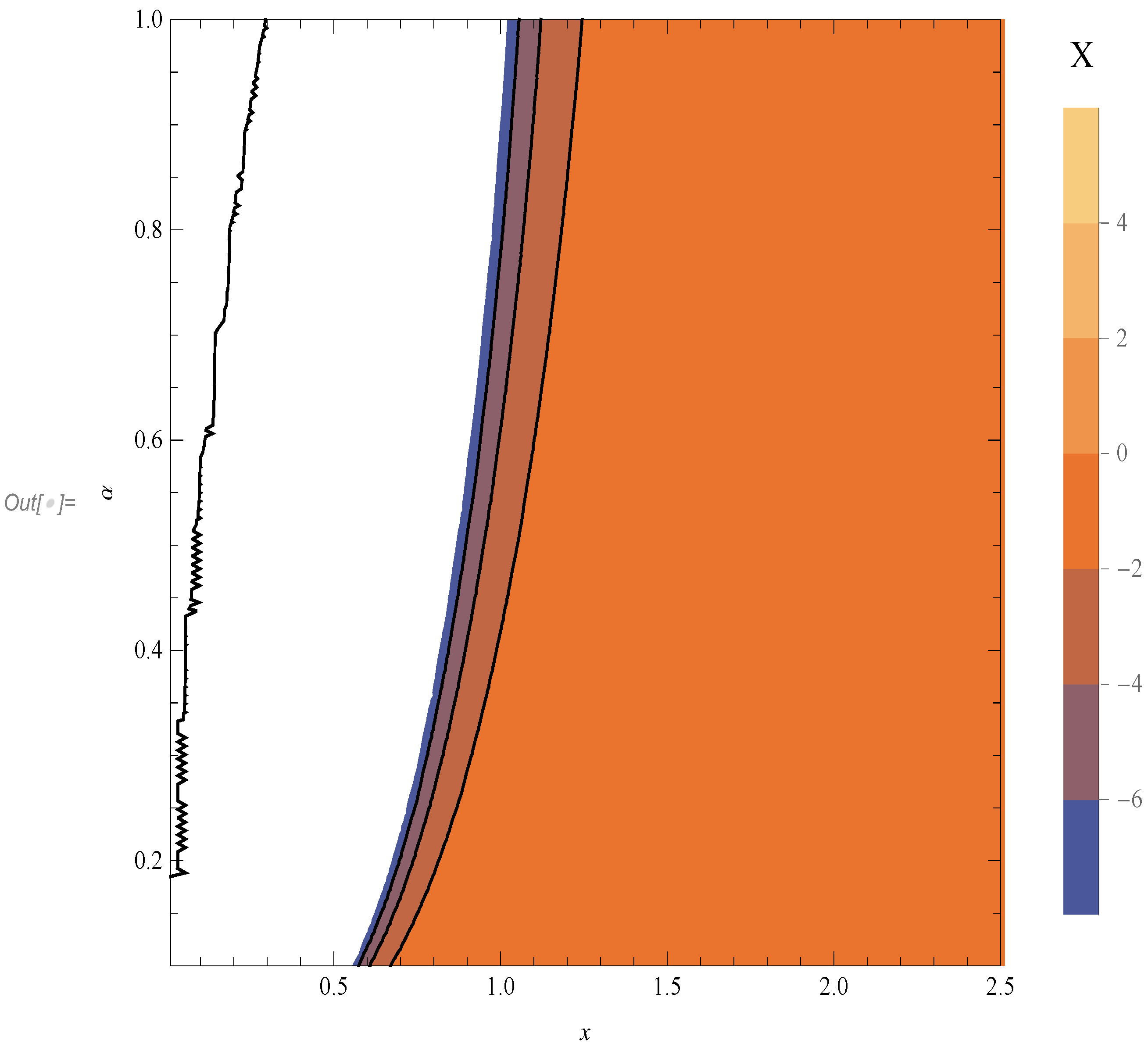
Now, the difference between the two is defined:

$$\begin{array}{c}X=X_{(RN)}-X_{(S)}=\frac{7}{2}\frac{{\alpha }^4}{x^8}-12\frac{{\alpha }^2}{x^7},\hfill \end{array}$$

(138)

and we provide the contour plot in the space of the two parameters $(\alpha ,x)$.

As can be inferred from Figure 1, the function X acquires negative values in the accepted parameter space. This means that $|X_{(S)}|>|X_{(RN)}|$; hence, we can “move” towards smaller values of x (or r) in the case of Reissner–Nordström rather than that of Schwarzschild, before the curvature “blows up” to infinity. In some sense, the addition of the electromagnetic field (a point charge) leads to a more localized singularity around the value $r=0$, and hence, by this criteria, a “less” singular spacetime.

To this end, we are going to compare the classical Reissner–Nordström and the quantum corrected one (QRN) based on the above described method. To proceed, the constant $l_p$ is redefined in terms of $r_s$ as follows $l_p=\frac{r_s}{\beta }$, where for $\beta \to 0$, the classical Reissner–Nordström is retrieved. The quantum RN has many divergent terms, but we keep only the higher ones, which coincide in powers of r with those of the classical solution. For completeness,

$$\begin{array}{cc}\hfill & X_{(QRN)}=X_{(RN)}+\frac{23}{4}\frac{{\left({\alpha }^2\beta \right)}^2}{x^7}+\frac{{\left(\alpha \beta \right)}^2}{x^6}\left\{-\frac{37}{2}+{\alpha }^2\left[\frac{1}{2}+\frac{111}{16}{\beta }^2-\frac{9}{8}{\left(\alpha \beta \right)}^2\right]\right\},\hfill \end{array}$$

(139)

$$\begin{array}{cc}\hfill & X=\frac{23}{4}\frac{{\left({\alpha }^2\beta \right)}^2}{x^7}+\frac{{\left(\alpha \beta \right)}^2}{x^6}\left\{-\frac{37}{2}+{\alpha }^2\left[\frac{1}{2}+\frac{111}{16}{\beta }^2-\frac{9}{8}{\left(\alpha \beta \right)}^2\right]\right\}.\hfill \end{array}$$

(140)

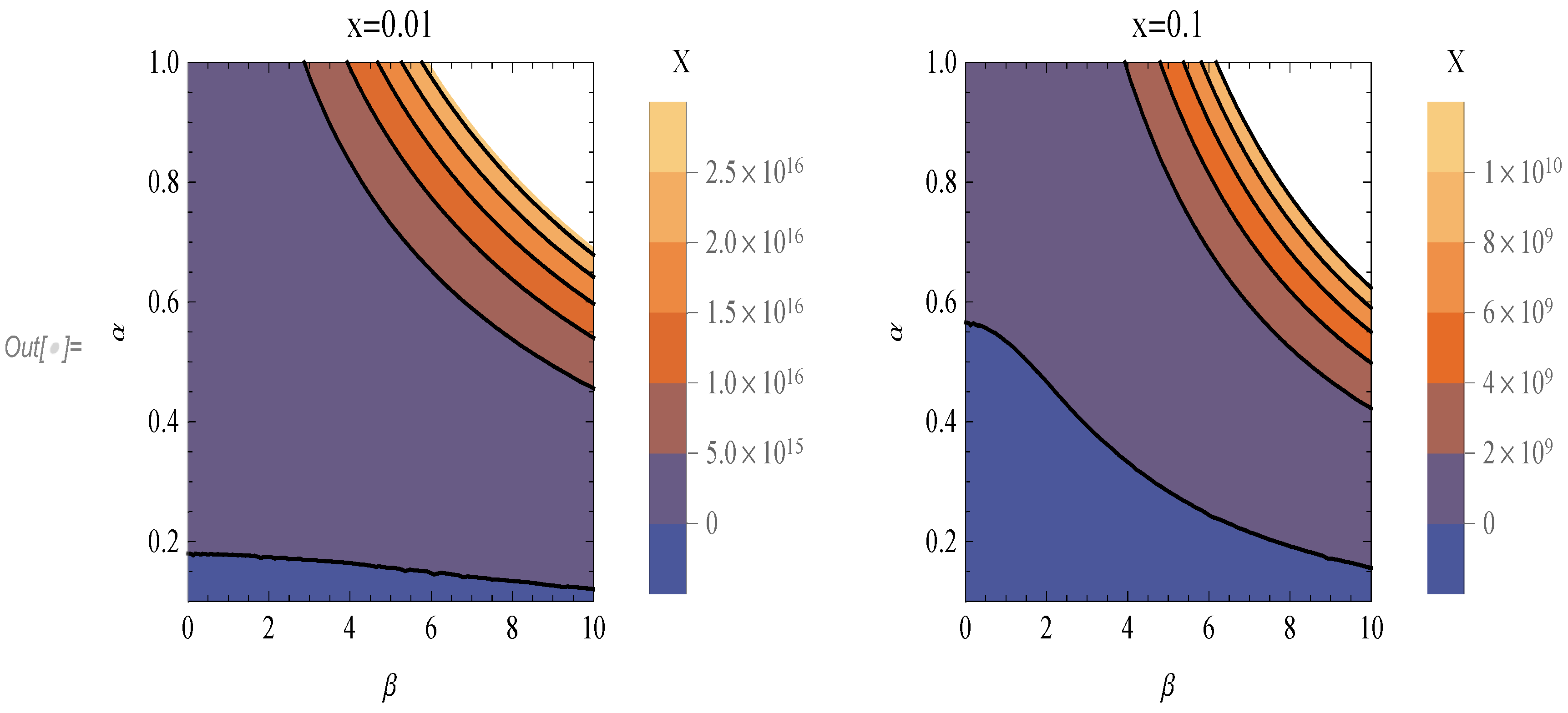
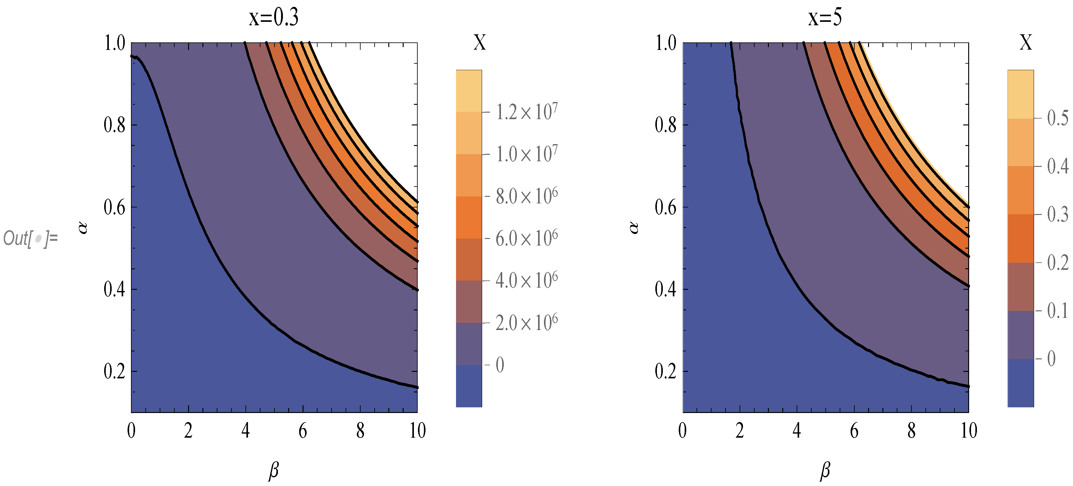
Now, the space of parameters is three-dimensional; thus, we could give a density plot. However, in trying, we found out that it is not very presentable. Thus, we decide to construct some contour plots in the space of variables $(\alpha ,\beta )$ for some specific values of x. The results are presented in Figure 2 and Figure 3.

Some remarks are at hand: The first thing that we observe is that there are values of the parameters that imply $|X_{(QRN)}|>|X_{(RN)}|$, meaning that the quantum corrected spacetime is “more” singular than the classical one based on the above criterion. The second thing is that in all four cases, there exists the deep blue region, which corresponds to $|X_{(QRN)}|<|X_{(RN)}|$ and, hence, a “less” singular spacetime. Finally, as we move closer to $(x=0)$, the desired region becomes smaller. Therefore, we can always achieve “less” singular spacetimes for some values of $\beta$, but the characteristics of those black holes (encoded in $\alpha$) are bounded to specific values. If we now focus on a specific distance x, then we observe that as $\beta$ grows, meaning stronger quantum effects, the region of accepted values of $\alpha$ is closer to $\alpha =0$, which corresponds to a Schwarzschild black hole.

4.4. Event Horizons

This solution exhibits event horizons as the classical Reissner–Nordström solution. From (124), the solution $g_{00}(r)=0$ leads to the divergence of the second diagonal element of the metric tensor. There are four solutions to the above equation, but only two of them correspond to a positive sign for r. The result is:

$$\begin{array}{cc}\hfill & r_{+}^{(Q)}=r_{+}\sqrt{\frac{l_p^2}{l_p^2-r_{+}^2}},r_{-}^{(Q)}=r_{-}\sqrt{\frac{l_p^2}{l_p^2-r_{-}^2}},\hfill \end{array}$$

(141)

where $r_{\pm }$ are the usual Reissner–Nordström inner and outer horizons:

$$\begin{array}{cc}\hfill & r_{+}=\frac{1}{2}\left(r_s+\sqrt{-4r_q^2+r_s^2}\right),r_{-}=\frac{1}{2}\left(r_s-\sqrt{-4r_q^2+r_s^2}\right).\hfill \end{array}$$

(142)

There are some remarks worth mentioning.

• The existence of both inner and outer horizons is possible only if the following relations are true:

  $$\begin{array}{c}{l}_p>r_{+}.\hfill \end{array}$$

  (143)
• In the case $l_p=r_{+}$, there is only one horizon, which we are going to call $r_{(+-)}$:

  $$\begin{array}{c}{r}_{(+-)}^{(Q)}=\frac{r_{+}{r}_{-}}{\sqrt{r_{+}^2-r_{-}^2}}\iff r_{(+-)}^{(Q)}=\frac{r_q^2}{\sqrt{r_s}{\left(-4r_q^2+r_s^2\right)}^{1/4}}.\hfill \end{array}$$

  (144)
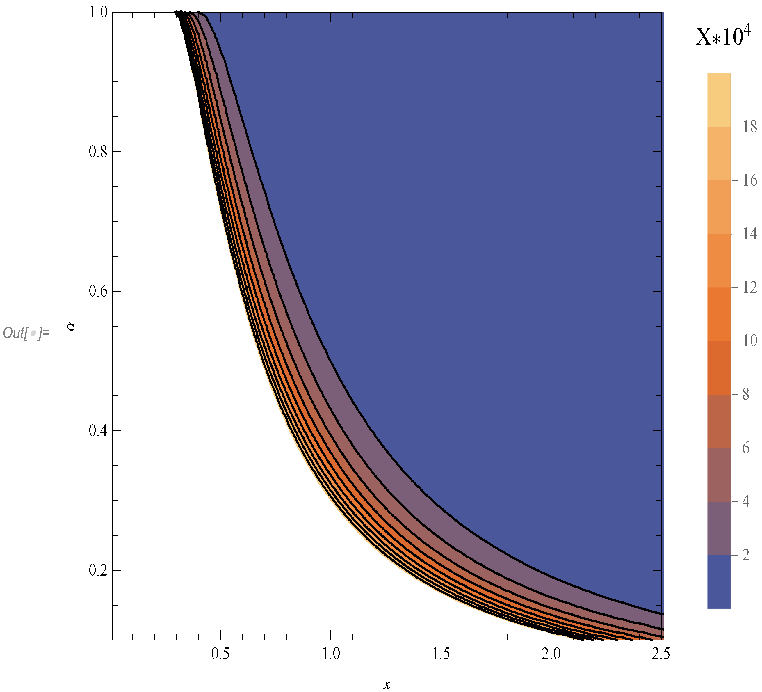
• In the case $l_p=r_{-}$, there is no horizon at all. Better expressed, the value of the coordinate r at which $g_{00}(r)=0$ is imaginary. For this particular value $l_p=r_{-}$, the parameter $\beta$ becomes a function of $\alpha$, $\beta =\frac{2}{1-\sqrt{1-{\alpha }^2}}$. In the absence of a horizon, we recognize the existence of a naked point singularity, since as can be inferred from Figure 4, there are no values $(\alpha ,x)$ for which $|X_{(QRN)}|<|X_{(RN)}|$.
• From the above, two remarks are that: As the quantum effects become stronger, meaning $l_p\to 0$, the horizons are vanishing. For instance, a black hole with $l_p>r_{+}$ would consist of a region $r\le r_{+}^{(Q)}$ where no information could escape. In the case $l_p=r_{+}$, this region is defined by $r\le r_{+-}^{(Q)}$. Since $r_{+-}^{(Q)}<r_{+}^{(Q)}$, information could escape from regions from which it could not before.
• There is also the extremal horizon for which $r_s=2r_q$, implying a degeneracy in this case as well:

  $$\begin{array}{c}{r}_{+}^{(Q)}=r_{-}^{(Q)}.\hfill \end{array}$$

  (145)
  This extremal case could not exist for the value $l_p=r_{+}$.
• In the accepted domain of $l_p$, in order for $r_{+}^{(Q)},r_{-}^{(Q)}$ to exist, we find that the following inequalities must hold:

  $$\begin{array}{cc}\hfill & r_{+}^{(Q)}>r_{+},\hfill \end{array}$$

  (146)

  $$\begin{array}{cc}\hfill & r_{-}^{(Q)}>r_{-}.\hfill \end{array}$$

  (147)
  Furthermore, an additional one holds for $l_p>\frac{r_{+}{r}_{-}}{\sqrt{r_{+}^2-r_{-}^2}}$:

  $$\begin{array}{c}{r}_{-}^{(Q)}>r_{+}.\hfill \end{array}$$

  (148)
  Thus, the horizons of the QRN are larger than those of the classical solutions.

5. Discussion

The primary purpose of this work is to construct a Schrödinger-like equation, instead of a Wheeler–DeWitt one, for the Reissner–Nordström black hole, which holds the property of being covariant, under reparametrizations of the defined “time” variable. To do so, a different procedure was followed from those appearing in the literature, to the best of our knowledge. Specifically, the singular Lagrangian density (23)–(25) describing the dynamics of the system was a function of the degrees of freedom $(a,b,\mathsf{\Phi })$ and the lapse n. The variation of the minisuperspace action integral with respect to n yields a constraint Equation (21), while dynamical equations appear from the variations with respect to the other degrees of freedom (18)–(20). Since many of the problems that appear in the quantization procedures are related to the existence of constraint equations, we thought that it is better if it did not exist, or better yet, if it were satisfied identically, once the solutions to the dynamical equations are obtained. One possible way to do so, without breaking the gauge freedom, is to solve the constraint equation with respect to the lapse function. To this end, from the reduced equations, only two of them are independent, (27) and (28), while there are three degrees of freedom left $(a,b,\mathsf{\Phi })$. We argued that this implies that the gauge freedom still exists, and we could have arrived at these two independent equations from the beginning, if somehow we were able to guess the proper form of the lapse as a function of the other degrees of freedom (26).

The reduced Lagrangian density has a square root form (32) and is still singular if $(a,b,\mathsf{\Phi })$ are all considered degrees of freedom. However, since there are only two independent equations (the third is satisfied once the other two are solved), these equations of motion can be reproduced via the variation of the action from the reduced Lagrangian density, with respect to only two of the degrees of freedom. There is the freedom to choose any of the pairs $(a,b)$, $(a,\mathsf{\Phi })$, or $(b,\mathsf{\Phi })$. We chose $(a,\mathsf{\Phi })$; hence, b is now considered as a mere function of the coordinate r and not a degree of freedom. To this end, the Lagrangian density is regular with respect to $(a,\mathsf{\Phi })$; it is “time” dependent due to the appearance of $b(r)$, and the gauge freedom still exists, encoded in the choice of $b(r)$. Note that due to the explicit position that $b(r)$ appears in the spacetime metric, we cannot gauge fix it to a constant value.

As we have pointed out, the Lagrangian density has a square root form, and as is known, problems will arise in the quantization procedure when the square root Hamiltonian density will have to be turned into an operator. To avoid such kinds of problems, we searched for a quadratic in the “velocities” Lagrangian density, which reproduces the equations of motion, and we succeeded in finding one (36)–(38).

Before moving to the quantum description, we noticed that the minisuperspace metric corresponds to a flat, Minkowski spacetime. This implies the existence of coordinates $(u,w)$ so that the minisuperspace metric acquires the diagonal form with eigenvalues $(-1,1)$. To this end, the reduced equations acquired a very simple form (44), and the solution in an arbitrary gauge was obtained, by solving one algebraic and one linear, second order, differential equation. We find that this is one of the simplest ways to obtain the solution in an arbitrary gauge.

At that point, a remarkable equivalence appeared: these equations of motion have exactly the same form and are equal in number, with the equations of motion for a 3D electromagnetic pp-wave spacetime, which we studied in some previous work [52]. This bizarre and interesting coincidence inspired us to assume that there might be a kind of classification of spacetimes+matter, based on the equivalence in the form of Einstein’s equations, with the underlying reason being the geometrical characteristics of the minisuperspace metric. This idea, however, will be pursued in some future work.

Obtaining the Hamiltonian density was an easy task. Note that since it is a “time”-dependent quantity, it is not conserved. However, there is the $H_{con}$ (66) and three Noether charges (67) that are conserved modulo the equations of motion. For the quantum description, we followed the canonical quantization procedure, meaning the elevation of observables into self-adjoint operators and the replacement of the Poisson brackets with the commutator. Since the Hamiltonian density is regular, the construction of a Schrödinger-like equation is possible. Furthermore, the hyperbolic nature of the Hamiltonian density operator implies that we have not defined an “intrinsic time” variable (we have not broken the gauge invariance). The idea is that we use as the parameter of “time” the coordinate (r), which appears explicitly in the Hamiltonian density through the function $M(r)$ (or $b(r)$ equivalently). This Equation (77) looks like a hybrid between the “intrinsic time” Schrödinger equation and the Wheeler–DeWitt equation that we described in the Introduction. The difference with the first lies in the “time”-covariance property; hence, the quantum descriptions for each different gauge choice are, by definition, equivalent. For the second, the difference appears in the evolution of states in our description, in contrast to the “frozen” picture related to the Wheeler–DeWitt equation. Note at this point that the word “time” was used nominally in the various places inside the text, since as is inferred from the line element, the variable r is a spatial coordinate. Alongside this, any reference to evolution of states is with respect to this external parameter r and should not be confused with the usual quantum mechanical sense of the evolution of states in time.

The solution to this equation was obtained for wavefunctions that are common to the operators ${\widehat{H}}_{con},{\widehat{Q}}_1,{\widehat{Q}}_2$. The evolution of two initial states was studied, Dirac’s delta and Gaussian. These two approach each other at a certain limit of the parameter that appears in the Gaussian distribution and control its width. For both cases, the wavefunctions were obtained, and the probability densities were calculated (96) and (103), respectively. In order to acquire some sense of the quantum corrections to the spacetime and interpret the wavefunctions in geometrical terms, the Bohm analysis was employed. The results are the following: For Dirac’s delta initial state, the quantum potential is zero; hence, the semi-classical “trajectories” coincide with the classical ones. The Gaussian initial state becomes a delta function only at a certain limit; hence, the obtained result is a non-zero quantum potential, resulting in different semi-classical trajectories from the classical “trajectories” (124)–(126). The quantum corrections manifest themselves as the appearance of an additional energy-momentum tensor $T_{\mu \nu }^{(Q)}$ and a four-current density $J_{(Q)}^{\mu }$ in the system of Einstein–Maxwell equations. Their explicit formulas can be found in (129)–(132). One important aspect of the semi-classical solutions is that they contain the classical solutions as a limit, specifically in the limit that $T_{\mu \nu }^{(Q)}$, $J_{(Q)}^{\mu }$ vanish.

As we pointed in the Introduction that one of the motivations to construct a quantum theory of gravity is for the purpose of “healing” the singularities from which the classical theory suffers. As we obtained in Section 4.3, the quantum corrected RN is still singular. One way to observe this is due to the Ricci scalar, whose appearance is solely due to $T_{\mu \nu }^{(Q)}$. For small values of the variable r, this object scales as $R\sim \frac{1}{r^3}$; hence, as $r\to 0$, the Ricci scalar tends to infinity. At that point, since for the classical RN solution, the Ricci scalar is zero, we found it more insightful to compare the Kretschmann scalars of these two spacetimes. We defined a criterion in order to adjudicate whether or not the situation gets better in the case of QRN regarding the divergence of the Kretschmann scalar. The criterion states the following:

Between two spacetimes that suffer from the same kind of singularity, in this specific case, a point-like, “less” singular one will characterize the one whose singularity is more localized around the point of interest.

Regarding the QRN and RN black holes, there are admissible values of the parameters for which QRN is “less” singular, as well as values for which is “more” singular. In the figures that are presented, there is a tendency that states that: as $\beta \to \infty$ (translated as stronger quantum effects, moving further away from Dirac’s delta distribution), the characteristics of these black holes that are encoded as values of $\alpha$ for which QRN is still “less” singular are close to zero. The upper value of $\alpha$ for a specific value of $\beta$ depends also on the proximity to the point $r=0$.

Another interesting result also related to the singularities is the following: Since we obtained a well-defined Hilbert space, and we calculated the probability densities, we may follow DeWitt’s proposal [23], which states that: if the wave function or, better, the probability density vanishes at the configuration points where the classical singularity appears, then it is avoided at the quantum level. The classical singularity appears for $r\to 0$, which translates into $\tau \to \infty ,\sigma \to \infty$. By carefully evaluating at this limit the probability densities for both cases of initial states, (96) and (103), we find that they are equal to zero. Hence, in light of the above proposal, the singularities disappear in the quantum regime. Therefore, a discrepancy appears between this result and the result obtained via Bohm’s analysis. One possible explanation might be that Bohm’s analysis is just an approximate scheme, with the approximation localized in the identification (110) of the classical and quantum momenta. A recent article discussing the singularity resolution and its dependence on the choice of clock can be found in [58].

Since we used the probability densities to comment on the existence of singularities, it is rather instructive to comment also on the possible interpretation of these probability densities. As we explained, the external parameter r is considered as the “time” variable in the Schrödinger equation. To this end, $P(r,\tau ,\sigma )={|\mathsf{\Psi }(r,\tau ,\sigma )|}^2$ is to be understood as the probability density for the variables $(\tau ,\sigma )$ at “time” r. This kind of interpretation is not unknown; it appears also in the “intrinsic time” formalism of the full quantum theory, where a multi-“time” Schrödinger equation is constructed. For more information, see [5]. In this particular work, we used symmetries to restrict ourselves to a minisuperspace model, which implies, due to the minisuperspace model at hand, that a spacelike parameter r remains to be interpreted as “time”. If a cosmological minisuperspace model were to be used instead, then the usual timelike coordinate t would appear. Regarding the collapse of the wave-function after some measurement we may say that the usual quantum mechanical interpretation could be used. Lastly, due to the lack of a complete physical theory of quantum gravity, it is far from obvious to know whether such a quantum minisuperspace model would appear as a limiting case of the full theory and, hence, render it physical. At this point in time, we would say that it is more of a mathematical model with a possible physical meaning through the use of the Bohmian interpretation; it might be possible to contrast the quantum corrected metric with observations.

Event horizons (inner and outer) also appear for QRN, under the assumption that the constant related to the quantum effects, $l_p$, satisfies the condition $l_p>r_{+}$, where $r_{+}$ is the outer RN horizon. In comparison with the event horizons of the classical solution, we found that they have a larger radius. The reason for that may be attributed as well to the presence of the additional energy-momentum tensor in the quantum corrected metric. There exists the case of extremal horizons as well. Furthermore, for different values of the parameter $l_p$, which controls the localization of $T_{\mu \nu }^{(Q)}$ and $J_{(Q)}^{\mu }$, there are the cases where two horizons exist, only one degenerate and none, implying a naked singularity. We observed that with the above defined criteria for the singularity resolution, the naked singularity does not disappear. Of course, let us point out once again that based on DeWitt’s proposal, there are no singularities at all. Hence, this is another strand of the revealed discrepancy. All the results that were obtained via Bohm’s analysis can be reduced to the Schwarzschild black hole by the simple substitution $r_q=0$. For future work, it may be interesting to study the geodesic equation and find the corrections that are imposed due to quantum effects. Furthermore, some experimental boundaries may be imposed on the values of the parameter $l_p$.

Finally, we believe that this “hybrid” procedure on the construction of a Schrödinger equation, for the case of minisuperspace models, will provide some new perspective on the problem of time. It is our intention to study, in some future work, other minisuperspace models as well and, perhaps, even try to formulate this procedure in the full theory of gravity.

6. Conclusions

Since the Discussion section is quite lengthy, we find it helpful to present in brief the important points.

• Reduction of the singular minisuperspace Lagrangian (Hamiltonian) density of the Reissner–Nordström black hole to a regular, “time”-dependent Lagrangian (Hamiltonian) density, without gauge fixing.
• Equivalence revealed at the level of equations, between the above described spacetime and a 3D electromagnetic pp-wave studied in previous work.
• Construction of a “time”-covariant Schrödinger equation, as a hybrid between the “intrinsic” time Schrödinger and Wheeler–DeWitt equation.
• Singularity criterion: “less” singular between two spacetimes is characterized by the one whose singularity is more localized around the point of interest.
• Discrepancy revealed concerning the existence of singularity, between the geometric origin, Bohm’s analysis, and DeWitt’s proposal (zero probability density at the classical singular point).

7. Materials and Methods

The Mathematica © software was used wherever it was needed.