How to Avoid Absolute Determinismin Two Boundary Quantum Dynamics

Abstract

Arguments for a two boundary theory are briefly outlined. Plausible concepts of how in such a theory an approximate causal macroscopic theory can emerge are presented. A problem with simple implementations of the two boundary theory is that effective or real willful decisions can not be added as there is no consecutive macroscopic time ordering. In this letter, we present a somewhat drastic but beautiful way to avoid it.

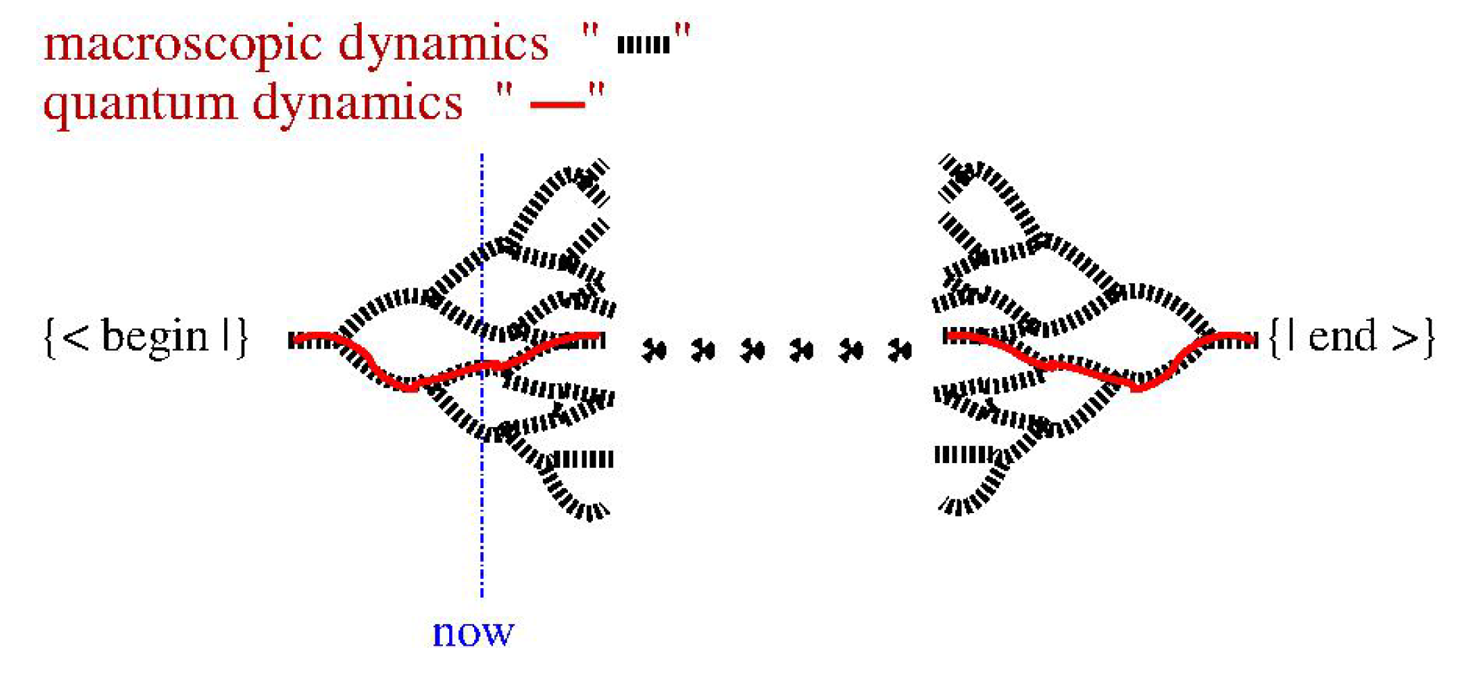
1. Two Boundary Quantum Dynamics

Quantum dynamics (quantum mechanics without measurement jumps [1]) is a non-relativistic limit of relativistic quantum field theory most likely with local interactions and must be considered as such.

It means relativity cannot be ignored. With ontological real waves and objective frequentist probabilities, Einstein, Podolsky, and Rosen’s experiment [2] means backward causation [3,4,5,6]. Questioning causality is, of course, more serious than denying locality [7,8,9,10].

It also means quantum statistical effects have to be considered [11]. In quantum statistics, a setting chosen at a time t can enhance or reduce the size of an interference contribution and its consequences are lying in the future and the past. It can involve astronomical time intervals. Consider the Hanbury Brown and Twiss observation of two photons emitted from a star observed with telescopes many light-years away. The interference contribution can have a positive value and the process is then statistically enhanced. In this situation the change in the setting reducing or eliminating the interference contribution can be done, say, one light-year away from the emitting star. It means that all conventional measurements in the star during this year have to be taken as provisional. The setting eventually chosen affects backward in time a tiny change in the available energy in the star depending on the emitted or not emitted photons. There is backward causation affecting the ontological probabilities of processes [4,12].

Measurements lead to macroscopic decisions. To be precise, there are three steps. Initially, possible components of an incoming state are separated at a furcation point (e.g., in a Stern–Gerlach experiment). In a subsequent decoherence phase, a huge number of witnesses are produced by each component (e.g., in drift chambers). The final collapse or jump part is the actual measurement. It seemingly random-selects one component, eliminates the not chosen contribution (i.e., to apply a projection operator), and renormalizes probabilities. With, anyhow, required backward causation, the removal of the wrong component up to the furcation point presents no problem. The collapse decision can be postponed to way behind the measuring device as the produced witnesses needed to identify the components to be selected or deselected can be assumed to be around practically forever.

On the star in the Hanbury Brown and Twiss consideration, final measurement decisions cannot occur before the setting is fixed. To avoid a complicated theory with a year of only provisional measurement results on the star we advocate a simpler way. It just postpones all measurements to the end of the considered time interval. Present-day physics is then described by pure quantum dynamics and deciding measurements appear only in the end.

Consider the evolution from an initial density matrix ${\rho }_{i^{*},i}$ to a final density matrix ${\rho }_{f,f^{*}}$ with a measurement device acting at an intermediate time $t.$ The deciding part of the measurement, the projection operator $\mathcal{M}$, is then postponed to the end of the interval, i.e., to $t_{\mathrm{final}}$, relying on available witnesses.

This basic concept can now be written in a more symmetric form. We can define a modified effective final density matrix:

$$\widetilde{{\rho }_{f,f^{*}}}=\mathcal{M}{\rho }_{f,f^{*}}\mathcal{M}.$$

including this measurement decision. We proceed to replace $\mathcal{M}$ with all the zillion measurement projection operators in the evolution of the universe except a considered not postponed ${\mathcal{M}}_1\left(t_1\right)$ and define

$$\tilde{\widetilde{{\rho }_{f,f^{*}}}}={\mathcal{M}}_2\cdots {\mathcal{M}}_{\mathrm{zillion}}{\rho }_{f,f^{*}}{\mathcal{M}}_{\mathrm{zillion}}\cdots {\mathcal{M}}_2-$$

In this way one obtains:

$${\mathrm{probability}}_{{\mathcal{M}}_1\left(t_1\right)}=\frac{Tr\left({\rho }_{i^{*},i}U({\tau }_i-t_1){\mathcal{M}}_1\left(t_1\right)U(t_1-{\tau }_f)\tilde{\widetilde{{\rho }_{f,f^{*}}}}{U}^{*}({\tau }_{f^{*}}-t_1){\mathcal{M}}_1\left(t_1\right)U^{*}(t_1-{\tau }_{i^{*}})\right)}{Tr\left({\rho }_{i^{*},i}U({\tau }_i-{\tau }_f)\tilde{\widetilde{{\rho }_{f,f^{*}}}}{U}^{*}({\tau }_{f^{*}}-{\tau }_{i^{*}})\right)}$$

a completely time-symmetric two boundary interpretation. This interpretation is advocated by many authors, including us [11,13,14,15,16,17,18].

It can be formulated in a somewhat simpler way if the final density matrix can be expanded in a reasonably convergent series of vector products:

$$\begin{array}{ccc}\hfill \widetilde{\tilde{{\rho }_{f,f*}}}& =& c_1·|f_1><f_1|+c_2·|f_2><f_2|+c_3·|f_2><f_3|\cdots .\hfill \end{array}$$

(1)

As the matrix contains zillions of projection operators, the coefficients have to be extremely tiny. Two statistically independent extremely small quantities cannot have the same magnitude. So in good approximation only the leading term has to be considered (“dominant state approximation”) and one can write:

$$\widetilde{{\rho }_{f,f}}=|\mathrm{f}><\mathrm{f}|.$$

The same can be assumed for the initial state:

$${\rho }_{i,i}=|\mathrm{i}><\mathrm{i}|.$$

The obtained two-state-vector formalism was carefully investigated for almost half a century by Aharonov and collaborators [19]. It contains no internal inconsistencies. With the caveat that one might have to go back to density matrices, we will use in the following this simpler formulation.

2. The Emerging Macroscopic Dynamics

The elephant in the room is how something like a macroscopic description can emerge in such two boundary quantum dynamics. Consider the basic situation. Available experimental observation tests quantum dynamics extremely well (by 16 digits) but in contrast, many things we think to know about classical physics might be wrong and just valid as a good approximation. Needed are just concepts of how an approximate Classical physics emerges [20]. Our argument has three parts.

2.1. No Classical Backward Causation

Firstly, the quantum statistical argument for backward causation does not involve typical classical observations. Contrary to the considered quantum processes “macroscopic measurements” involve more or less equal statistically enhanced and depleted components. So the net effect of changes in the settings affecting the weight of interference contributions vanishes. It does not mean that the argument for backward causation is only a theoretical construction [21,22,23,24,25].

2.2. The Breaking of the Time Symmetry

The second concept describes how the time symmetry of quantum dynamics is broken. Causal macroscopic dynamic involves a decision tree. A decision at one furcation determines the future. How can a non-causal theory underlie such a macroscopic causal decision tree with a time direction?

To explain our concept we start with a definition. A “Macroscopic State” $\left\{\right|q>\}$ is the sum/integral over all states macroscopically indistinguishable from $|q>$.

$$\left\{|q>\right\}=\sum _{\mathrm{all}\mathrm{states}\mathrm{macroscopically}\mathrm{consistend}\mathrm{with}|q>}|q_i>$$

It includes all possible phases between different components, etc.

The specified initial and final quantum states have only a tiny overlap as they incorporate all projection operators. They allow a unique macroscopic path from a macroscopic initial to a macroscopic final state. What happens if we replace the initial and final quantum state by their corresponding Macroscopic States. Now phases that tend to determine furcation decisions are open and multiple pathways appear, as it is shown in Figure 1.

There seems to be a problem. The initial Macroscopic State also describes the initial state in classical physics which predicts one unique pathway. Classical physics holds only approximately but it is pretty much known to hold on a time scale of the present age of our universe. The concept is that the total lifetime of the universe is much longer and the underlying QM allows then for many pathways consistent with Macroscopic initial and final States.

The resulting situation is depicted in Figure 1.

The source of our causal time direction is our asymmetric position in the universe, i.e., $\left({\tau }_{\mathrm{now}}-{\tau }_{\mathrm{big}\mathrm{bang}}\right)\ll \left({\tau }_{\mathrm{end}}-{\tau }_{\mathrm{now}}\right)$ [26,27]. The concept is that the past evolution is too short to enable macroscopic multiple pathways and that evolution in the future is long enough to allow for them. Decisions which appear now seem to have consequences in the future. The fact that decisions have to be consistent with the final macroscopic state is not noticeable. Of course, all decisions are in reality encoded in the final quantum state and the felt causality is fake.

The two boundary description is meant for the whole universe. For truly macroscopic measurements observable radio waves are emitted from the circuit boards (or the brain of say Schrödinger’s cat). The energy of a radio frequency photon is unobservable ${10}^{-26}$ Joule. So there are a lot of them and enough will escape the box, the house, and the ionosphere to reach the dark sky. They will then no longer encounter interactions and reach the end of the considered two boundary quantum dynamics interval, i.e., the end of the universe.

To illustrate the decisiveness of the vastly extended final state one can reverse the time and evolve it backward. A very large number of its radio photons will reach the particular area of the decoherence phase of the measurement where they originated (e.g., the drift chamber) clearly determining the decision at the furcation point.

2.3. Consecutive Willful Decisions

The considered two boundary QM is absolutely deterministic [28]. In the first view, it looks not bad. It is your willful decision to read this letter. It could actually mean that you change the final boundary to result in your decision about the present situation. Your free will would be nicely hidden neurologically in seemingly random quantum jumps. However, each tiny decision would require recalculating the entire universe. Also within the final state, the time ordering of my decision to write and yours to read is not intrinsically available. So this way to avoid determinism is not acceptable.

What is meant with absolutely or inescapably deterministic? Classical physics is deterministic but not inescapably deterministic. To allow for willful decisions the theory can be amended. At a given time there can be a possible interaction of an individual with the neurons of his brain. For two such interactions, there is a well defined consecutive time order. In contrast, this escape from determinism is not possible in the inescapably deterministic concept considered above. If an operation is entered at a time t it will have only consequences on a quantum level. The fixed final state still contains unchanged witnesses of all macroscopic decisions. Also, there is no intrinsically consecutive time-relation to a second operation.

Speculations aside there seems to be no fully acceptable solution to how willful decisions operate and what they mean [29]. They can be real willful interventions or they can be quantum effects in the brain [30], which somehow appear as our sudden decisions. Nevertheless, there is no doubt about the time structure. The requirement of a consecutive order should be taken as a serious requirement. Can one obtain it in a two boundary QM?

The basic idea is to avoid the fixed final state and to replace it by a just matching one. We discuss it in a simple cosmological framework of a big bang big crunch universe. The total age of the universe is taken to be $\tau$ and both the expanding and the contracting phase is assumed to last for $\tau$/2.

As above, all quantum decisions are stored in the initial and final state. Their overlap:

$$<\mathrm{bang}|\mathrm{crunch}>=〈{(\begin{array}{c}\mathrm{evolved}\\ \mathrm{bang}\end{array})}_{\tau /2-ϵ}\left|{(\begin{array}{c}\mathrm{revolved}\\ \mathrm{crunch}\end{array})}_{\tau /2+ϵ}\right.〉\sim 2^{-\#\mathrm{all}\mathrm{decisions}}$$

is extremely tiny. As in the initial consideration, the longevity of witnesses allows us to move all projection operators of effective measurement-collapse decisions for the expanding part to just before and for the collapsing part with its flipped time to just after the border position. In this way the indicated “evolved bang” and the “revolved crunch” are obtained with a unitary operation.

No “fine-tuning” is involved as no big number is created dynamically. At the border, the extremely extended universe has only a tiny fraction of fermion-mass sized non-vacuum states. So matching is extremely rare. This allows the following approximation. We define something like a density function connecting the incoming and outgoing states:

$${\rho }_{\max .\mathrm{extend}}=\sum _{i,j}\rho (i,j)|\begin{array}{c}\max .\\ \mathrm{extend}\end{array}\left(i\right)><\begin{array}{c}\max .\\ \mathrm{extend}\end{array}\left(j\right)|.$$

With the above argument, its smallness means that only a single component dominates, i.e., we can just approximate it as:

$${\rho }_{\max .\mathrm{extend}}\sim |\mathrm{border}><\mathrm{border}|.$$

For the total evolution, it leaves two factors:

$$<\mathrm{bang}\left|U\right|\mathrm{border}>\otimes <\mathrm{border}\left|U\right|\mathrm{crunch}>$$

The first factor corresponds to the concept considered above with the final state replaced by the border state. In our epoch, say at a time t, all macroscopic decisions are determined by the border state acting as an effective final state.

No time arrow is accepted, so the contracting world is analogous to the expanding one. The common quantum border state determines the same macroscopic pathways at t or resp. at $\tau -t$. To avoid problems with strange duplicities we introduce the surjection hypothesis where macroscopic states are taken to extend from $[0,\tau /2]$ while the quantum states are defined in $[0,\tau ]$. Macroscopic objects then live with their wave function $\psi \left(t\right)$ in the “expanding” phase with their more or less CPT conjugate wave function ${\psi }^{*}(\tau -t)$ in the “contracting” phase.

A willful agent can now introduce operators at his macroscopic time $t\sim \tau -t$ without otherwise changing the quantum dynamics:

$$\begin{array}{ccc}\hfill \psi \left(t\right)& ⟼& \tilde{\psi }\left(t\right)=\mathrm{Operator}\left[\psi \left(t\right)\right]\hfill \\ \hfill \psi (\tau -t)& ⟼& \tilde{\psi }(\tau -t)={\mathrm{Operator}}^{\mathrm{CPT}}\left[\psi (\tau -t)\right]\hfill \end{array}$$

In consequence $\psi$ changes mainly in the macroscopic future, i.e., from the initial path

$$<bang|\sim \sim \sim \sim \sim \sim \sim \sim \sim \sim \sim \sim \sim \sim \sim \sim \sim \sim \sim \sim \sim \sim |crunch>$$

to the desired path shown as translation

$$<bang|\sim \sim \left[\mathrm{Operator}\left(\mathrm{t}\right)\right]\stackrel{\sim \sim \sim \sim \sim \sim \sim }{\phantom{(}}\left[Operator(\tau -t)\right]\sim \sim |crunch>.$$

A second willful decision at the time $t^{\prime }\sim \tau -t^{\prime }$ with $t^{\prime }>t$ will encounter the modified situation. In this way, the theory allows for a consecutive order of outside interventions and it is no longer absolutely deterministic

In principle the matching at the border changes, which can affect $\psi$ everywhere. However, as $t\ll \tau$ the change in the macroscopic past can be neglected [29].

The concept eliminates an annoying aspect of QM. Consider the “Stern–Gerlach experiment” shown in Figure 2.

As a macroscopic object, the apparatus lives in both phases. The drift chambers shown as blue boxes create enough witnesses to exclude mixed “up”/“down” contributions. Both the red path and the yellow one contribute. Their sizes—before the overall normalization—are tiny by many orders of magnitude and it is statistically impossible that they have the same magnitude and one choice will dominate completely.

The choice reflects unknown properties of the available future path. The apparent randomness of QM disliked by Einstein [31] found a beautiful deterministic explanation. The absence of predictable correlations suffices for the usual statistical mechanics type of considerations.

On average both contributions are equal. It does not include the size of the up and down component in the entering states. As this factor appears twice in both phases, the “Born rule” holds [32]. It is no longer a quantity of matching properties but a direct consequence of the physical process.

3. Conclusions

The considered two boundary theory has no internal quantum paradox. A plausible concept of how an approximate causal macroscopic theory can emerge is presented. Unfortunately, it is absolutely deterministic, which seems hard to accept. In this letter, we presented a somewhat radical but beautiful way out. It was explained for a simple cosmological evolution.

The real universe should of course have a more complicated topology with a non-directed time defined along a suitable path. Most of the time a macroscopic description might not be available. However, our epoch should be an exception as a joint expansion and contraction lead to a region determined by the same border state so that the proposed mechanism for a macroscopic description works. In any case, the different initial and final states will eventually make a macroscopic description unavailable, which has serious consequences for our understanding of the early universe [33,34].

References

1. Sakurai, J.J.; Napolitano, J.J. Modern Quantum Mechanics; Pearson Higher Ed.: London, UK, 2014. [Google Scholar]
2. Einstein, A.; Podolsky, B.; Rosen, N. Can quantum-mechanical description of physical reality be considered complete? Phys. Rev. 1935, 47, 777. [Google Scholar] [CrossRef] [Green Version]
3. Wharton, K.; Argaman, N. Colloquium: Bell’s theorem and locally mediated reformulations of quantum mechanics. Rev. Mod. Phys. 2020, 92, 021002. [Google Scholar] [CrossRef]
4. Evans, P.W. Retrocausality at no extra cost. Synthese 2015, 192, 1139–1155. [Google Scholar] [CrossRef] [Green Version]
5. Leifer, M.S.; Pusey, M.F. Is a time symmetric interpretation of quantum theory possible without retrocausality? Proc. R. Soc. Math. Phys. Eng. Sci. 2017, 473, 20160607. [Google Scholar] [CrossRef]
6. Rietdijk, C. Proof of a retroactive influence. Found. Phys. 1978, 8, 615–628. [Google Scholar] [CrossRef]
7. Stapp, H.P. Nonlocal character of quantum theory. Am. J. Phys. 1997, 65, 300–304. [Google Scholar] [CrossRef]
8. Shimony, A.; Stein, H. Comment on “Nonlocal character of quantum theory,” by Henry P. Stapp [Am. J. Phys. 65 (4), 300–304 (1997)]. Am. J. Phys. 2001, 69, 848–853. [Google Scholar] [CrossRef]
9. Mermin, N.D. Nonlocal character of quantum theory? Am. J. Phys. 1998, 66, 920–924. [Google Scholar] [CrossRef] [Green Version]
10. Vaidman, L. Quantum nonlocality. Entropy 2019, 21, 447. [Google Scholar] [CrossRef] [Green Version]
11. Bopp, F.W. An intricate quantum statistical effect and the foundation of quantum mechanics. arXiv 2019, arXiv:1909.01391. [Google Scholar]
12. Aharonov, Y.; Cohen, E.; Elitzur, A.C. Can a future choice affect a past measurement’s outcome? Ann. Phys. 2015, 355, 258–268. [Google Scholar] [CrossRef] [Green Version]
13. Hartle, J.B. Arrows of Time and Initial and Final Conditions in the Quantum Mechanics of Closed Systems Like the Universe. arXiv 2020, arXiv:2002.07093. [Google Scholar]
14. Cramer, J.G. The transactional interpretation of quantum mechanics. Rev. Mod. Phys. 1986, 58, 647. [Google Scholar] [CrossRef]
15. Bopp, F.W. A Bi-directional Big Bang/Crunch Universe within a Two-State-Vector Quantum Mechanics? Found. Phys. 2019, 49, 53–62. [Google Scholar] [CrossRef] [Green Version]
16. Bopp, F.W. Time Symmetric Quantum Mechanics and Causal Classical Physics. Found. Phys. 2017, 47, 490–504. [Google Scholar] [CrossRef] [Green Version]
17. Bopp, F.W. Causal Classical Physics in Time Symmetric Quantum Mechanics. In Proceedings of the 4th International Electronic Conference on Entropy and Its Applications, Basel, Switzerland, 21 November–1 December 2017. [Google Scholar] [CrossRef] [Green Version]
18. Wharton, K. Time-symmetric boundary conditions and quantum foundations. Symmetry 2010, 2, 272–283. [Google Scholar] [CrossRef] [Green Version]
19. Aharonov, Y.; Bergmann, P.G.; Lebowitz, J.L. Time symmetry in the quantum process of measurement. Phys. Rev. 1964, 134, B1410. [Google Scholar] [CrossRef]
20. Carroll, S.M.; Singh, A. Mad-Dog everettianism: Quantum mechanics at its most minimal. In What Is Fundamental? Springer: Berlin, Germany, 2019; pp. 95–104. [Google Scholar]
21. Peres, A. Quantum Theory: Concepts and Methods; Springer Science & Business Media: Berlin, Germany, 2006; Volume 57. [Google Scholar]
22. Sondermann, M.; Maiwald, R.; Konermann, H.; Lindlein, N.; Peschel, U.; Leuchs, G. Design of a mode converter for efficient light-atom coupling in free space. Appl. Phys. 2007, 89, 489–492. [Google Scholar] [CrossRef] [Green Version]
23. Hellmuth, T.; Walther, H.; Zajonc, A.; Schleich, W. Delayed-choice experiments in quantum interference. Phys. Rev. 1987, 35, 2532. [Google Scholar] [CrossRef]
24. Jacques, V.; Wu, E.; Grosshans, F.; Treussart, F.; Grangier, P.; Aspect, A.; Roch, J.F. Delayed-choice test of quantum complementarity with interfering single photons. Phys. Rev. Lett. 2008, 100, 220402. [Google Scholar] [CrossRef] [Green Version]
25. Davidson, M. On the Mössbauer Effect and the Rigid Recoil Question. Found. Phys. 2017, 47, 327–354. [Google Scholar] [CrossRef] [Green Version]
26. Bedingham, D.J.; Maroney, O.J. Time reversal symmetry and collapse models. Found. Phys. 2017, 47, 670–696. [Google Scholar] [CrossRef] [Green Version]
27. Dente, G.C. Causality in the Classical Limit for Quantum Electrodynamics. Found. Phys. 2018, 48, 628–635. [Google Scholar] [CrossRef]
28. Hossenfelder, S.; Palmer, T. Rethinking superdeterminism. Front. Phys. 2020, 8, 139. [Google Scholar] [CrossRef]
29. Hooft, G.T. The free-will postulate in quantum mechanics. arXiv 2007, arXiv:quant-ph/070109. [Google Scholar]
30. Plenio, M.B.; Huelga, S.F. Dephasing-assisted transport: Quantum networks and biomolecules. New J. Phys. 2008, 10, 113019. [Google Scholar] [CrossRef]
31. Vaidman, L. Quantum Theory and Determinism. Quant. Stud. Math. Found. 2014, 1, 5–38. [Google Scholar] [CrossRef] [Green Version]
32. Vaidman, L. Derivations of the Born rule. In Quantum, Probability, Logic; Springer: Berlin, Germany, 2020; pp. 567–584. [Google Scholar]
33. Castagnino, M.; Fortin, S.; Laura, R.; Sudarsky, D. Interpretations of quantum theory in the light of modern cosmology. Found. Phys. 2017, 47, 1387–1422. [Google Scholar] [CrossRef] [Green Version]
34. Hartle, J.B. The Impact of Cosmology on Quantum Mechanics. arXiv 2019, arXiv:1901.03933. [Google Scholar]
Figure 1. The macroscopic view of the universe.
Quantumrep 02 00030 g001
Figure 2. Stern–Gerlach experiment.
Quantumrep 02 00030 g002